Calhoun: The NPS Institutional Archive

Theses and Dissertations Thesis Collection

1981

Development of improved finite elements formulation

for shallow water equations.

Woodard, Edward T.

Monterey, California. Naval Postgraduate School

http://hdl.handle.net/10945/20493

:•••••'

BmXMwv

HMSHMS*

H C I

mKw%

DUO'.' LI "'.ARY

1JATE SCHOOL

I'.IF, 93940

NAVAL POSTGRADUATE SCHOOLMonterey, California

THESISDEVELOPMENT OF IMPROVED

FINITE ELEMENT FORMULATIONSHALLOW WATER EQUATIONS

FOR

by

Edward T. Woodward

September 1981

Thesis Advisors: R.T.

U.R.

WilliamsKodres

Approved for public release; distribution unlimited.

T204559T20A560

SECURITY CL AIII'ICATIOM OF THIS »»GE (Whan Dim Em.r.di

REPORT DOCUMENTATION PAGE READ INSTRUCTIONSBEFORE COMPLETING FORM

1 IIH1T NUMltH 2. GOVT ACCESSION NO. 1 RECIPIENT'S CAT ALOG NUMBER

4 TITLE «n* Submit)

Development of Improved Finite ElementFormulation for Shallow VJater Equations

S. TYPE OF REPORT ft PERIOO COVEREDMaster's ThesisSeptember 1981

«. PERFORMING ORG. REPORT NUMBER

7 A _--.?» J

Edward T. Woodward

1 CONTRACT OR GRANT NUMBERS)

t »(M9UING ORGANIZATION NAME AND AOORESS

Naval Postgraduate SchoolMonterey, California 93940

10. PROGRAM ELEMENT. PROJECT TASKAREA ft WORK UNIT NUMBERS

11 CONTROLLING OFFICE NaUI AMO AOORESS

Naval Postgraduate School

Monterey, California 93940

12. REPORT OATE

September 198111. NUMBER OF PAGES

170

T4 MONlTORlNS AGENCY NiMC k AOOHIIM/ Uttfrmnt tram Contra'tUnf Slltca) IS. SECURITY CLASS. o( thia ripori)

IB* DECLASSIFICATION' DOWNGRADINGSCHEDULE

I*. DISTRIBUTION STATEMENT 'ol thf *rpo"

Approved for public release; distribution unlimited

'7 DlSTRiBU T ION STATEMENT at ina •attract anlarad In Black 20. II dlllararti *•• * apart)

It SuPPL EmEnTARY NOTES

It. <EY WORDS CMilnut on tarataa tlda II nacaaaarr and Idamttty PF Black ->umtbmn

Finite elements piecewise constant basis functionShallow water equations primitive barotropic equationsVoriti city-divergence formulation Galerkin methodSemi -implicit numerical prediction model

piecewise linear basis function variable size elementsJO ABSTRACT fC«iilmM on ravaraa ..a. // nacaaaarr ana Idamiltr kw 'lock mammar)

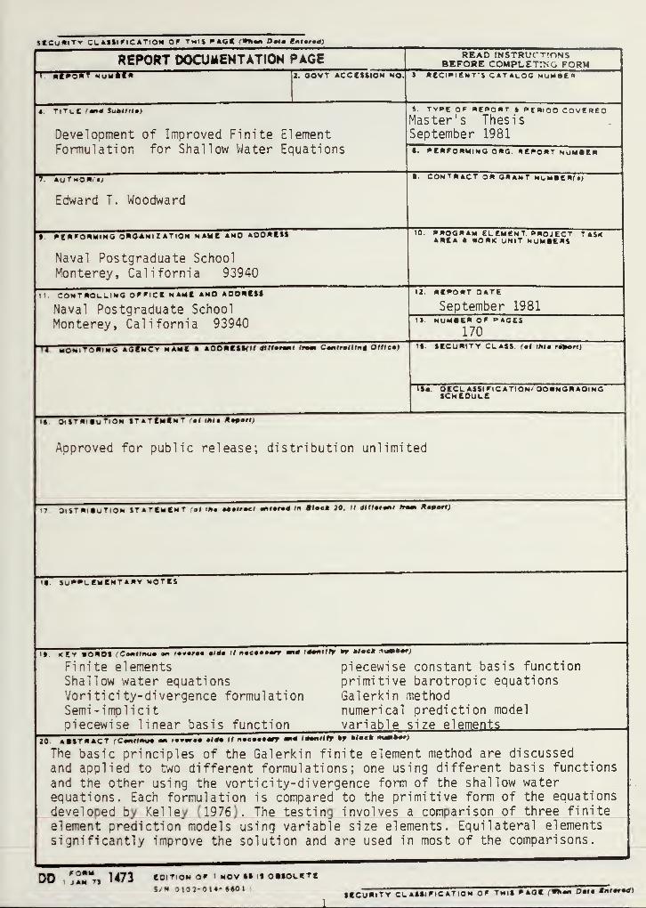
The basic principles of the Galerkin finite element method are discussedand applied to two different formulations; one using different basis functions

and the other using the vorti city-divergence form of the shallow waterequations. Each formulation is compared to the primitive form of the equations

developed by Kelley (1976). The testing involves a comparison of three finiteelement prediction models using variable size elements. Equilateral elementssignificantly improve the solution and are used in most of the comparisons.

DOFORM

I JAN 7 , 1473 EDITION OF 1 NOV •• IS OBSOLETI

S/N 102-0 14- 4S0 1

SECURITY CLASSIFICATION OF THIS PAOE (Wkmm Data Kntatod)

^cuwt» cl«iiihc»"9ii a* Twit »m>*»»i n»n »«—

«

The formulation using different basis functions produces poorer results than

the primitive formulation. The vorti city-divergence formulation producessuperior results while executing faster than the primitive model. However,it does require more storage and the relaxation parameters are sensitiveto the domain geometry. The computer implementation for the vorticity-divergence model is discussed and the source listing is included.

DD FornQ 1473

Approved for public release; distribution unlimited

DEVELOPMENT OF IMPROVEDFINITE ELEMENT FORMULATION FOR

5 HAL LOW -V. ATE? EQUATIONS

by

Edward T. WoodwardCaptain. United States Air ForceB.A., University of Maine, 1970

Submitted in partial fulfillment of therequirements for the degrees of

FASTER OF SCIENCE IN COMPUTE? SCIENCEand

MASTER OF SCIENCE IN METEOPOLCSY

from the

NAVAL POSTGRADUATE SCHOOLSeoterrber 1981

abstract -°«war*The basic principles of the Galerkin finite element

method are discussed and applied to two different

formulations* one using different basis functions and the

other using the vorticity—divergence forrr of the shallow

water equations. lach f angulation is compared to the

primitive form of the equations developed by lelley (1976).

The testing involves a comparison of three finite element

prediction models using variable size elements. Equilateral

elements significantly improve the solution and are used in

most of the comparisons. The formulation using different

basis functions produces poorer results than the primitive

formulation. The vorticity-divergence formulation produces

superior results while executing faster than the primitive

model. Fcwever, it does require more storage and the

relaxation parameters are sensitive to the domain geometry.

The corputer implementation for the vorticity-divergence

model is discussed and the source listing is included.

TA3LE OF CONTENTS

I . INTRODUCTION 11

A. 3ACKGRCTJNE 12

2. OBJECTIVES 15

:. THESIS STRUCTURE 17

II. FINITE ELEMENTS 19

A. FINITE ELEMENT CONCEPT 2Z

2. GALERKIN APPLICATION 25

C. APIA COORDINATES 31

III. SHALLOW-WATER MOTEL 35

GOVERNING EQUATIONS 3?

ECUATION FORMULATION 39

7T V F DISCRETIZATION 41

COMPUTATIONAL TBCENIQUE 43

GRII GEOMETRY 45

INITIAL CONE IT IONS 47

50UNDART CONDITIONS 49

IV. COMPUTER IMPLEMENTATION 52

A . PROGRAM ARCHITECTURE 53

1. v ain Prograrr 55

2. Initialization Phase 56

3. Forecast Phase 64

3. UTILITY ^OIULES 65

V. PRIMITIVE "ODEL EXPERIMENT 63

A. v 0~EL DESCRIPTION 69

3. RESULTS 73

VI. LINEARIZE! MODEL EXPERIMENT 76

A. EQUATION REFORMULATION 78

P. RESULTS 81

Til. TORTICITY-BIVERGENCE MODEL EXPERIMENTS 34

A. TEST DOMAINS AND INITIAL CONDITIONS 84

B. TEST CASE COMPARISONS 87

1. Regular Case 87

2. Srcooth Case 91

3. Atruut Case 102

C. COMPUTATIONAL SENSITIVITY 105

Till. CONCLUSIONS 109

APPENDIX A 'Source List) Ill

A. DEFINITIONS Ill

3. MAIN PROGRAM 114

C. INITIALIZATION PEASE 115

D. FORECAST PHASE 141

Z. UTILITY PROGRAMS 151

LIST OP REFERENCES 167

INITIAL DISTRIBUTION LIST 159

LIST OF FIGURES

Figure 1

.

F i gu ~e 2

.

Figu re 3.

Figure 4.

Figure r"

.

Figure 6.

Figure n.

Figure 3.

Figure 9.

Figure 12

Figure 11

Figure 12

Figure 13

Figure 14

Figure IS,

Figure 16

Figure 1?

Figure 13

Fiecewise linear basis function 23

Basis and test function interactionluring the piecewise integrationore cess 27

Basis function for node 23 30

"artesian versus area coordinates 32

Transformation to area coordinates 32

Domain divided into equilateraltriangles 46

3 dirensional view of the initialfields 48

Assemble and store the coefficientmatrix for elerrent 3 62

Tomain divided into right triangles 71

Initial fields for the primitive""<)lel 72

46 hour forecast comparison betweenequilateral and right triangularelements 74

Differently shaped basis functions 77

Staggering the geopotential aboutthe velcci ty 79

Initial fields for the linearizedexperiment 32

48 hour forecast comparing theprimitive vs linearized model S3

Test domain geometries 35

Initial field for the Regular Case 86

48 hour forecast comparison for theRegular Case 39

7

r :^':re 19.

Figv.re 22.

Ji^ure 21.

Figure 22.

Figure 23.

Figure 24.

Figure 25.

Figure 26.

Figure 27.

Figure 28.

Initial field for the Smooth CaseA? A = 1.1 ir/s 92

48 hour forecast comparison for theSmooth Case A?A = 1.1 rr/s 93

Initial fields for the Smooth CaseA?A = 5.5 rr/s 95

4? hour forecast com-oarison for theSmooth Case, API = 5.5 m/s 96

96 hour forecast comparison for theSmooth Case, APA = 5.5 m/s 97

Initial fields for the Smooth CaseAFA = 1.1 m/s, 2 waves 1ZZ

46 hci;r forecast comparison for theSmooth Case, 2 waves.". 101

Initial fields for the Abrupt Case 123

43 hour forecast comparison for theAbrvpt Case 104

Computational sensitivity using the*e hour Vorticity field 127

3

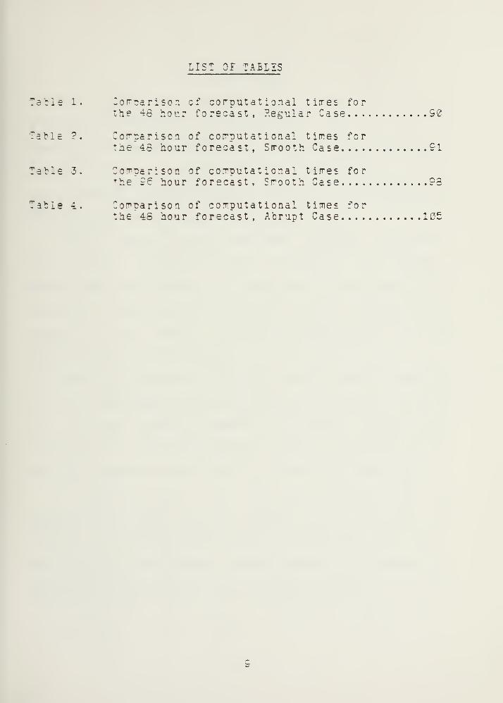
LIST OF TABLES

Table 1. -oirparison of corputat ional tiires forthe 46 hour forecast, Regular Case S0

Table ?. Comparison of computational times forthe 48 hour forecast, Sirooth Case 91

Table 3. CoTparison of corputat ional tirres for*he 26 hour forecast, Srooth Case 93

Tahle 4. Comparison of computational times forthe 45 hour forecast, Abrupt Case 105

c

ACKNOWLEDGEMENTS

The author telives that most of the credit should go to

Professor R.T. Williams for the education that he gave me

through his patient teaching and guidance during the entire

research and writing of this paper. Acknowledgement is also

due Professor U.R. Kodres for the many useful suggestions,

encouragement and reading the manuscript.

Special thanks to each department chairman, Professor

B.H. 3radley f Computer Science, Professor R.J. Renard,

Meteorology, and Professor !J.J. Ealtiner, former Meteorology

chairman, for allowing me to pursue the two degrees and

accepting this thesis as partial fulfillment for the

requirement? of "both degrees.

Thanks are extended to Lt. R.G. Kelley whose research

was the forerunner to this investigation and Capt. M. Cider

*or the many useful comments he offered during the

implementation. Particular thanks to Dr. M.J. P. Cullen whose

personal suggestions provided the direction for this work.

I give my love to my wife, Joy, for her Infinite

patience, for being the first guinea pig in reading and

preparing this manuscript. Finally, to my family, Kim, Mark

and Joy thanks for enduring and encouraging me throughout my

graduate studies at the Naval Postgraduate School.

10

I. INTHOrUCTION

Shuman fl978) claims that progress in numerical modeling

cf the general circulation has been to some degree dictated

in the past "by the rate of development in the field of

computer technology. Eowever, the limited ability to

Darameterize the effects of small-scale processes in terms

of large scale motions has been an equally important

limiting factor. Essentially, the major problem of numerical

modeling of the general circulation is simply that of

producing a very long range numerical weather forecast.

Certainly the equations used in the models must be more

sophisticated to include those physical processes- which are

unimportant for a short range forecast, but may become

crucial as the length of the forecast is extended. Another

area where concentrated efforts have improved the forecast

involves the computational techniques employed to

approximate and solve the governing equations of the models.

The motivation behind this thesis is to investigate the

application of a relatively new computational technique to

the field of numerical weather prediction. The finite

element method, long established in engineering, has been

seriously considered only during the past decade In

meteorology. This method has great potential for application

in atmosoheric Prediction models.

11

A. BACKGROUND

The rrost common numerical integration procedure for

weather prediction has been the finite difference method in

which the derivatives in the differential equations of

motion are replaced by finite difference approximations at a

discrete set of points in space and time. The resulting set

of equations, with appropriate restrictions, can then he

solved by algebraic methods. Until recently, the finite

difference method has been the workhorse in atmospheric

prediction models, from their first computer implementation

to the present .

With the introduction of each new generation of

computers. the gap between numerical forecasts and

atmospheric observations has decreased. The rate at which

this gap decreased has slowed down and appears to be

leveling off. This would indicate that computer technology

may not be the prirrary obstruction to better numerical

forecasts. In fact, bigger and faster computers alone have

demonstrated their inability to significantly improve the

numerical forecast.

7cr example, a major limiting factor of finite

difference approximations is the truncation error. The

National leather Service 7 Layer Primitive Equation P-odel

(7LPZ Model), operational from 1966 to 1980. had truncation

errors which increased at a rate proportional to the square

o*" the grid spacing. That is, the smaller the grid interval,

12

the siraller the truncation error. To increase its accuracy

would require increasing the grid matrix density. This would

require increased computer storage and computational tiire.

State of the art computers are capable of providing these

additional resources.

The problem now goes beyond numerical techniques and

romputer technology. Operationally, the National Weather

service is not capable (due to monetary restrictions) of

providing a denser concentration of atmospheric

observations. Therefore, with the present density of initial

data ( observations) and objective analysis techniques

(getting the data for grid points by interpolating from

observed data sources), reducing the grid spacing further on

the 7LPZ Model does not significantly increase the accuracy

of the solution.

This additional computer capability can not be utilized

usin«? finite difference methods. Therefore, new numerical

integration techniques must be investigated, such that given

the same density of observed data, superior solutions are

produced .

Two alternative techniques, the spectral method and the

finite element method, have started to gain attention. Both

the spectral and finite element methods require more

computational time per forecast time step than does the

finite difference method. For example, the finite element

method requires an equation solver to invert a larger matrix

13

at each tirre step for each variable. In this sense, these

methods were held hack by computer technology, hut recent

advances in computer technology (i.e. larger and faster

storage devices, multi-processors, etc) have made these

alternative numerical techniques competitive.

For long range weather predictions, the spectral method

applied over the globe or hemisphere is a natural method,

due to the existence of efficient transforms for the

nonlinear terms on spherical geometry. It also eliminates

the truncation error for the horizontal space derivatives

and the nonlinear instability (aliasing). For these reasons,

global spectral models have been developed, and implemented

on an operational level, replacing the global finite

difference models .

Eowever, because the spectral harmonics are globally

rather than locally defined, it is thought that for problems

of more detailed limited area forecasting, the finite

element method is more suitable. Pioneering work to adapt

finite element methods to meteorological applications has

been done by Cullen (1973,1974 and 1979), Staniforth and

Mitchell '1977), Kinsman (1975) and lelley (1976). The most

recent finite element meteorological model at the Naval

Postgraduate School was written by Kelley (1976) with the

-?llaboration of Tr. R.T. Williams. It is this study that

will serve as a basis for this thesis. The model written by

Kelley will be altered and used for comparative testing with

14

irproved finite element fortrs implemented by this author.

Some of the techniques and coles developed by Keliey are

also employed in this thesis. Older (1981) developed a

technique to smoothly vary the grid geometry in the domain.

This technique is also implemented both on Kelley's model

and vith the new formulation to give greater versatility

when testing the model performance.

3. C3J2CTI7ES

The objectives for this thesis can be divided into two

categories: 1) meteorology, 2) computer science. First, the

meteorological objectives of developing improved finite

element forms for shallow water equations are as follows:

1) - Older (1981) after collaboration with Dr.

M.J. P. Cullen, showed how equilaterally shaped elements

produced significantly better results than did other

triangular elements, ^elley (1976) used right triangular

elements in the implementation of a two-dimension.al finite

element model using the primitive form of the shallow water

equations. A considerable amount of small-scale noise was

observed in the solution. Hereafter, this model, which was

developed by lelley (1975), will be referred to as the

primitive model. This first objective involves

re-implementing the primitive model using equilaterally

shaped elements and comparing the results to those in

Zelley's thesis.

15

2^ - v illiaT>s and Zienlciewicz (1981) presented new

finite elerrent techniques for formulations for the shallow

water equations, which use differently shaped functions to

approximate the different dependent variables, which in

effect stagger the variables. Schoenstadt (1980)

demonstrated the advantage of spatial staggering of

dependent variables in finite difference models. The

application of this technique to finite element models is a

natural extension, and excellent results were obtained by

Williams and Zienkiewicz (1981) from application of these

r.ew formulations on linearized one dimensional cases. The

objective here is to implement the new forms on the

primitive jodel and again do quanitative comparisons of the

results

.

?) - The major emphasis in this study deals with the

implementation and comparison of the vorticity divergence

for'r of the shallow water equations, which is described in

detail in Chapter III. This formulation has the following

advantages. First, the geostrophic adjustment process is

treated better than in the primitive form of the equations.

Secondly, the velocity and height fields are evaluated at

the same grid point, where the best primitive form requires

staggering these dependent variables. And thirdly, a larger

time step is allowed due to the semi implicit form of the

equation. Again comparisons between the results from the

vorticity divergence and primitive model are presented.

16

The computer science aspect of this thesis was primarily

devoted to the implementation of the different models and

the style and architecture of the program. Finite element

methods require more computational time than do finite

difference methods, not only in the solution of the

equations, but also in the amount of computation required to

evaluate each term in the equations.

The implementations of these two dimensional models,

although complex when viewed from the surface, have a lot of

generality and redundancy in the operations required.

Versatile modules can he written to ease the implementation

and facilitate changes. The objective here is to efficiently

implement these new forms and demonstrate tne utility of

these versatile modules for future implementations.

C. THZSIS STRUCTURE

This thesis presents the results obtained from tests of

the various finite element formulations. The results are

compared to those from the primitive model written by Celley

(1976). Accompanying the results is a detailed discussion of

the reformMiation and implementation process.

Chapter II of the thesis presents a tutorial of the

finite element method and the area coordinates system used

in the evaluation of the element integration. The Galerkin

finite element method used in all the models is developed

and applied to the advection equation in one dimension.

1?

rhapter in presents the detailed description cf the

vcr f i ri ty-di vergence shallow water model. Here the equations

are shown and written using the Salerkin method. A

discussion of the computational technique used is presented

along with the -model's physical parameters.

Chapter IV presents a descriptive overview of the

computer implementation. The chapter includes a list of

options available for testing, a brief description of the

iratrij compaction technique and the formulations of the

versatile modules used to implement the complex equations.

Chapters V through VII discuss the results obtained fror

the different experiments. Chapter V briefly describes the

primitive model used for all comparisons and the results

froffl changing the element shape to equilateral triangles.

Chapter VI reformulates the primitive model so that the

geopotential is staggered with respect to the velocity

variable. Jor simplicity, the continuity equation is also

linearized. Chapter VII compares the results from the

vert icity-di vergence model developed in Chapter III to those

:"rom the primitive model.

The last chapter summarizes the results from all the

experiments and identifies what areas require follow on

work. The source code for the vorticity-divergence model is

presented in Appendix A.

16

II - FIN ITS 5LZMINTS

As is often the case with an original development, it is

rather difficult to quote an exact date on which the finite

element method was invented, but the roots of the method can

be traced tack to these separate groups: applied

mathematicians, physicists and engineers. Since the early

developments of the finite element method, a large amount of

research has been devoted to the technique. However, the

finite element method obtained its real impetus by the

independent developments carried out by engineers. Its

essential simplicity in both physical interpretation and

mathematical form has undoubtedly been as much- behind its

popularity as is the digital computer which today permits a

realistic solution of even the most comolex situations.

The name finite element was coined in a paper by

R.V. Clough, in which the technique was presented for plane

stress analysis, as discussed in Bathe (1976). While finite

element methods have made a deep impact via the field of

solid mechanics, where it can be said that today they

represent the generally accepted method of discretizing

continuum problems for computer-based solution, the same

appears not to be true in fluid mechanics or atmospheric

ored ic tion .

19

Numerous finite element formulations are currently

available. Strang (1973), Ncrrie (1973) and Zienkiewicz

11571} present detailed theoretical discussions of each. The

Galerkir. method , the most popular finite element method, is

described in detail below and used in the equation

formulation later.

A. FINITE ILZMINT CONCEPT

The problem of solving partial differential equations

can be specified in one of two ways. In the first, finite

difference methods specify the dependent variables at

certain grid points in space and time, and the derivatives

are evaluated using Taylor series approximations. Secondly,

the calculus of variation requires the minimization of a

functional over a domain, where a functional is defined as a

variational integral over the domain.

The calculus of variation approach creates a purely

physical model where the functional equivalent to the known

differential equations are lenown. Its major disadvantage is

that it limits the method only to those problems for which

fun'Uionals exist. Finite element methods, an extention of

this method. derive mathematical approximat icns directly

fror the differential equations governing the problem. The

advantage here is that it extends the method to a range of

problems for which a functional may not exist, or has not

been ii sc ove red .

2d

The finite eleirent rrethod divides the domain into

subdorains or finite elements (usually of the sarre form).

v.Mes are located along the boundary of the elements,

usually at the element vertices and at strategic positions

(mid! side, centroid, etc.) in the interior and on the sides

of faces of eletrents.

Commonly used elements are triangular, polygonal or

polyhedral in form for two-dimensional problems. The choice

of elements depends on the type of problem, the number of

elements desired, the accuracy required and the available

computing time. To begin with, the element must be able to

represent derivatives of up to the order required in the

solution procedure, and to guarantee continuous first

derivatives across the element boundaries to avoid

singularities. Triangular elements are errployed in this

thesis because they can be used effectively to represent

irregular boundaries, and/cr geometry, and also to

concentrate coordinate functions in those regions of the

domain where rapidly varying solutions are anticipated.

Consider the problem of solving approximately the

differential equation

L(u) = f(x II-l

where I is a differential operator, u the dependent

variable, and f(x) is a specified forcing function. Suppose

that II-l is to be solved in the dorrain a * x - b and that

21

appropriate boundary conditions are provided. The residual P.

is forced fror II— 1 as follows:

L(u) - f(x) = R II-2

The critical step is to select a trial fairily cf

approximate solutions (the members of a trial family are

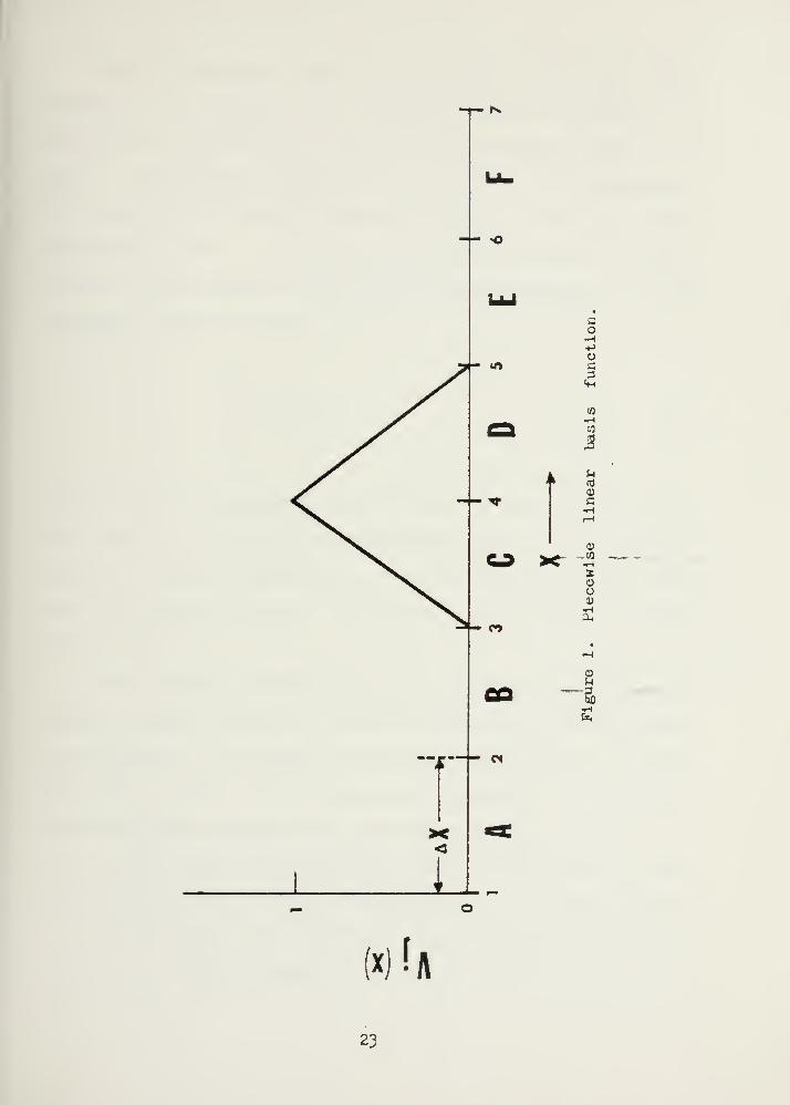
often called basis functions). The basis function is

prescribed 'functionally) over the domain in a piecewise

fashion, element by element, and are generally a combination

of low order polynomials . A one dimensional example is

shown in Figure 1, wherein the domain (x axis) is divided

into six elements (line segments) A through F. The basis

functions are linear and one is shown for node 4 only in

Figure 1.m he function has a value of unity over node 4, and

decreases linearly to is zero at nodes 3 and 5 and zero

els swhere.

Consider a series of linearly independent basis

functions V. (x), as in Figure 1. Now u(x) can be

approximated with a finite series as follows:

u(x) = Z $. V. (x) = 0.V.\ J J J J

where £ is the coefficient of the jth basis function and hasj

a value equal to u at node j.

Substituting this approximate solution I 1-3 wherever u

appears in the differential equation 1 1 —

1

L^.V.) - f(x) = R

22

II-4

so

-poc3Cm

I

0)

-03X" ^ —

(x)U

g-a•H

23

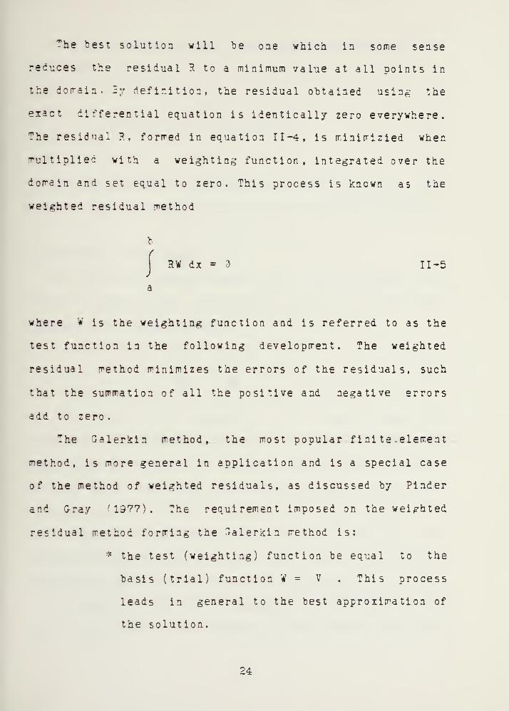
The best solution will be one which in some sense

reduces the residual R to a minimum value at all points in

the domain. By definition, the residual obtained using the

exact differential equation is identically zero everywhere.

The residual P., formed in equation II-4, is minimizied when

multiplied with a weighting function, integrated over the

domain and set equal to zero. This process is known as the

weighted residual method

b

RV dx = 3 II-5\

where W is the weighting function and is referred to as the

test function in the following development. The weighted

residual method minimizes the errors of the residuals, such

that the summation of all the positive and negative errors

add to zero

.

The ^alericin method, the most popular fini te element

method, is more general in application and is a special case

of the method of weighted residuals, as discussed by Pinder

ar.d Gray ^1977). The requirement imposed on the weighted

residual method forming the ^alerkin method is:

* the test (weighting) function be equal to the

basis (trial) function W = V . This process

leads in general to the best approximation of

the solution.

24

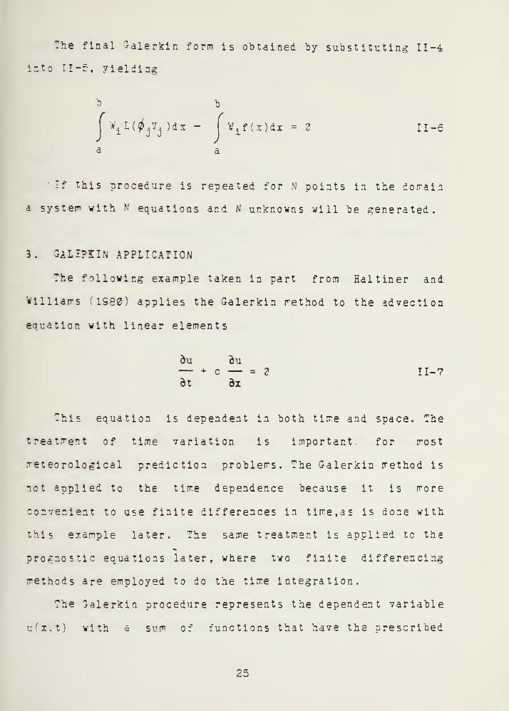
The final (Jalerkin form is obtained by substituting II-4

into II-5, yielding

-fi

±l((j}.l. )dx - Vf

1f (x)dx = II-S

If this procedure is repeated for N points in the domain

a system with N equations and N unknowns will be generated.

3. OAimiN APPLICATION

The following example taken in part from Haltiner and

Williams (1980) applies the Galerkin rethod to the advection

equation with linear elements

du du— + c — =2at dx

II-7

This equation is dependent in both time and space. The

treatment of time variation is important for most

meteorological prediction problems. The C-alerkin method is

not applied to the time dependence because it is more

convenient to use finite differences in time f as is done with

this example later. The same treatment is applied tc the

prognostic equations later, where two finite differencing

methods are employed to do the time integration.

The 7alerkin procedure represents the dependent variable

u'x.t) with a sum of functions that have the prescribed

25

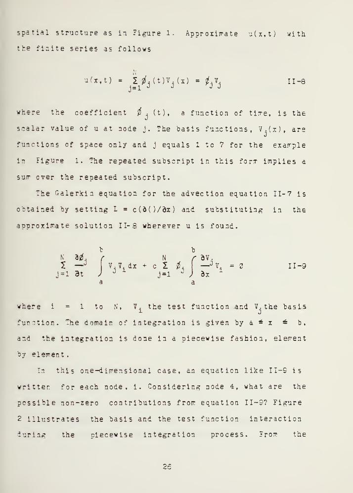
spatial structure as in Figure 1. Approximate u(x,t) with

the finite series as follows

u(x f t) = I rf.(t)V .(i) = 0.?,1 = 1^ ^ ^ *J

II-8

where the coefficient . (t), a function of tirre, is the

scalar value of u at node j. The basis functions, V.(x), are

functions of space only and j equals 1 to ? for the example

In Figure 1. The repeated subscript in this forx implies a

sun- ever the repeated subscript.

The Galerkin equation for the advection equation II-7 is

obtained by setting L = c(d()/dl) and substituting in the

aooroximate solution II- 8 wherever u is found.

N

1j=i at

*0Am J

b

r N

V.V. dx + c I (. —JV,

dx]

II-9

where i = 1 to N v V. the test function and V.the basis

function. The domain of integration is given by a * x - b,

and the integration is done in a piecewise fashion, element

by element

.

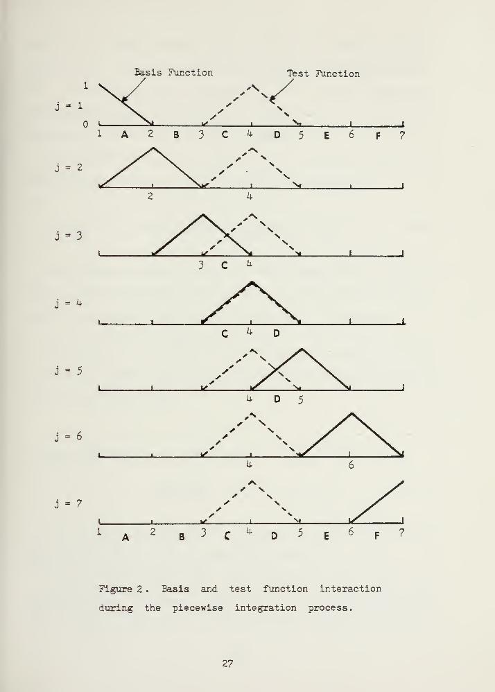
In this one-dimensional case, an equation like 1 1—9 is

written for each node, i. Considering node 4, what are the

possible non-zero contributions from equation 1 1—9? Figure

2 illustrates the basis and the test function interaction

luring the piecewise integration process. From the

25

j - 1

i

Basis Function

s

Test Function

^t.

J = 2

1A2B3C^D5E6F7

J - 3

3 C ^

= 4

J - 5

= 6

C ^ D

,'%

4 D 5

J - 7

1 A 2B 3 C

^ D 5 E 6 F 7

Figure 2 . Basis and test function interaction

during the piecewise integration process

.

27

definition of the basis and the test function, locally

defined as unity at node j and linearly decreasing to zero

; ± 1 and zero elsewhere, the only non—zero

contributions are made when * = 3 over element C, j - 4 ever

elements ~ and ?, and j = 5 over element D.

The evaluation of 1 1-9 for i = m, which is given in

Haltinep and Williams (1981), leads to the equation:

6 dtm+1

4u + u1 ) + e ( u

1- u m - ) = 11-10

in m-1 m+1 m-12-*x

The boundary points, which in this example are nodes 1

and 7, are evaluated in the same way as the interior nodes,

with the exception that cyclic conditions are imposed.

The time discretization of II—10 is d-one using- a finite

difference scheme. Applying leapfrog time differencing gives

the following equation

f

12 At m+1 m+1 m m

n+1m-1

n-1 ,

m-l

Hi m+1) = n-ii

The resultant equation set, in matrix form, contains an

NxN matrix where N is the number of nodes.

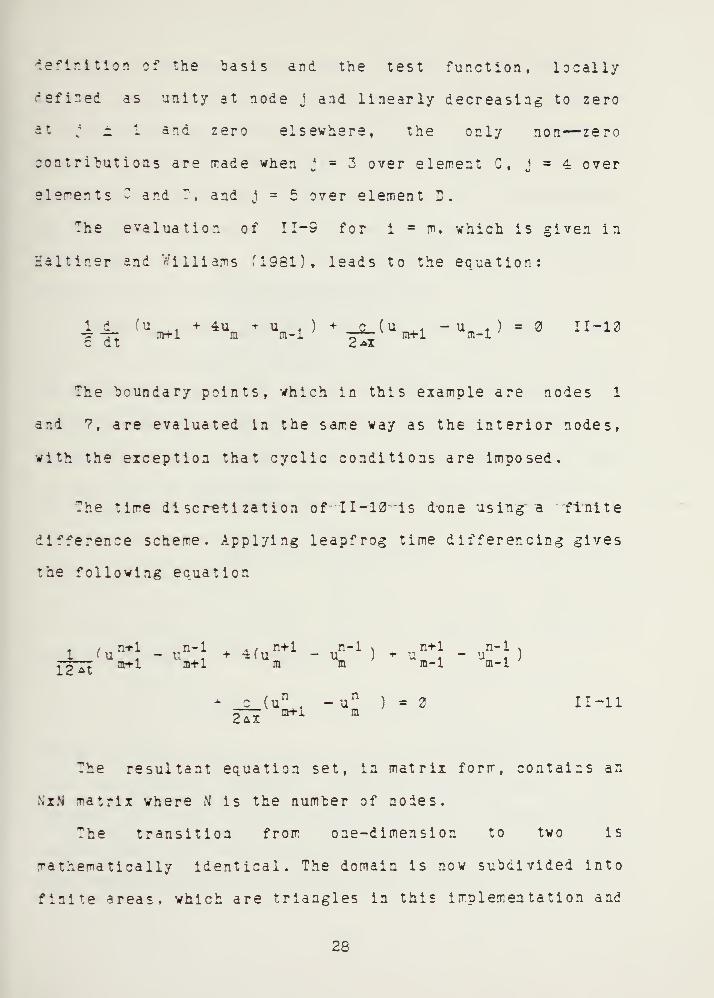
The transition from one-dimension to two is

mathematically identical. The domain is now subdivided into

finite areas, which are triangles in this implementation and

28

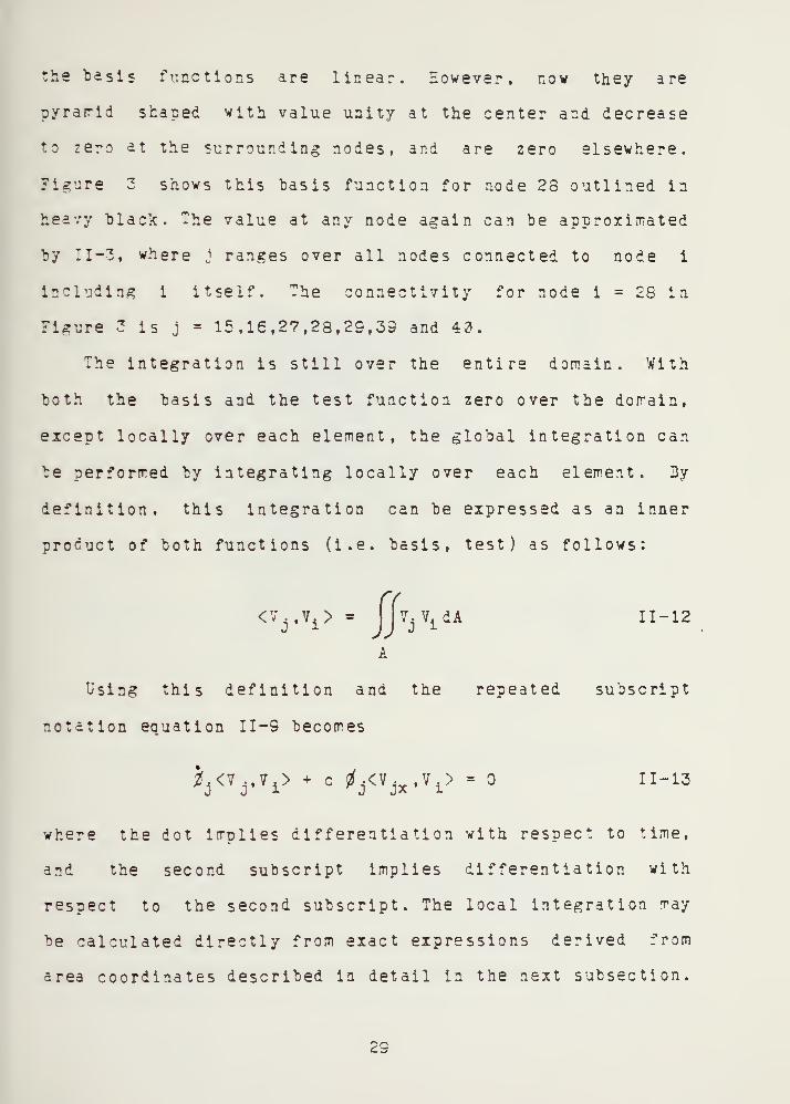
the basis functions are linear. However, now they are

pyrarid shaped with value unity at the center and decrease

to zero at the surrounding nodes, and are zero elsewhere.

Figure 2 shows this basis function for node 28 outlined in

heavy black. The value at any node again can be approximated

by II-3, where j ranges over all nodes connected to node i

including i itself. The connectivity for node i = 28 in

Figure 2 is j = 15,16,27,28,29,39 and 40.

The integration is still over the entire domain. With

both the basis and the test function zero over the domain,

except locally over each element, the global integration can

be performed by integrating locally over each element. By

definition, this integration can be expressed as an inner

product of both functions (i.e. basis, test) as follows:

<w =re

))A

V . V, dA

Using this definition and the repeated

notation eauation II—9 becomes

11-12

subscript

»-<?„?!> c iM*.X<> = 11-13

where the dot implies differentiation with respect to time,

and the second subscript implies differentiation with

respect to the second subscript. The local integration may

be calculated directly from exact expressions derived from

area coordinates described in detail in the next subsection.

C6

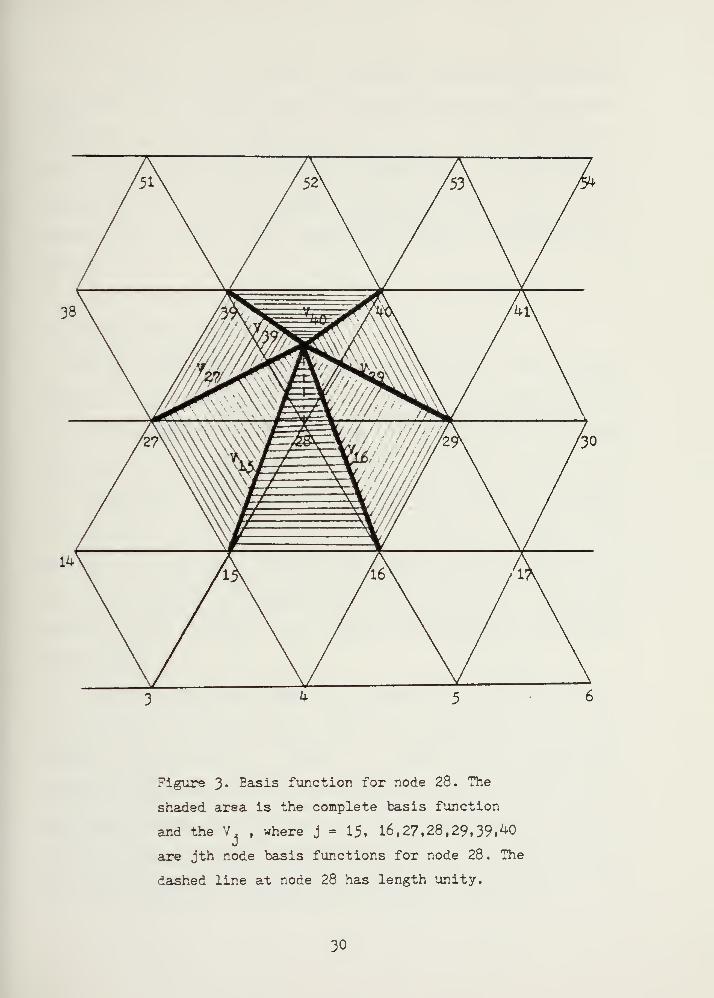
Figure 3. Basis function for node 28. The

shaded area is the complete basis function

and the V. , where j = 15, 16,27,28,29,39,^0

are jth node basis functions for node 28. The

dashed line at node 28 has length unity.

30

In sunwary, the Galerkin procedure involves subdividing

the domain into finite elements, approximating the dependent

variables by a linear combination of low order polynomials

a~A substituting them into the equations. The equation is

multiplied by a test function, integrated over the entire

domain and finally the resulting system of equations is

solved .

C. APIA COORDINATES

While the Cartesian coordinate system is the natural

choice of coordinates for most two dimensional problems, it

is not convenient when working with triangularly shaped

elements. It is therefore necessary to define a special set

of normalized coordinates for a triangle. Area, or natural

coordinates as they are commonly called, reduce the

formidable task of integrating products between the basis

avA test functions and their derivatives over a triangular

element and result in easily computable and exact

expressions .

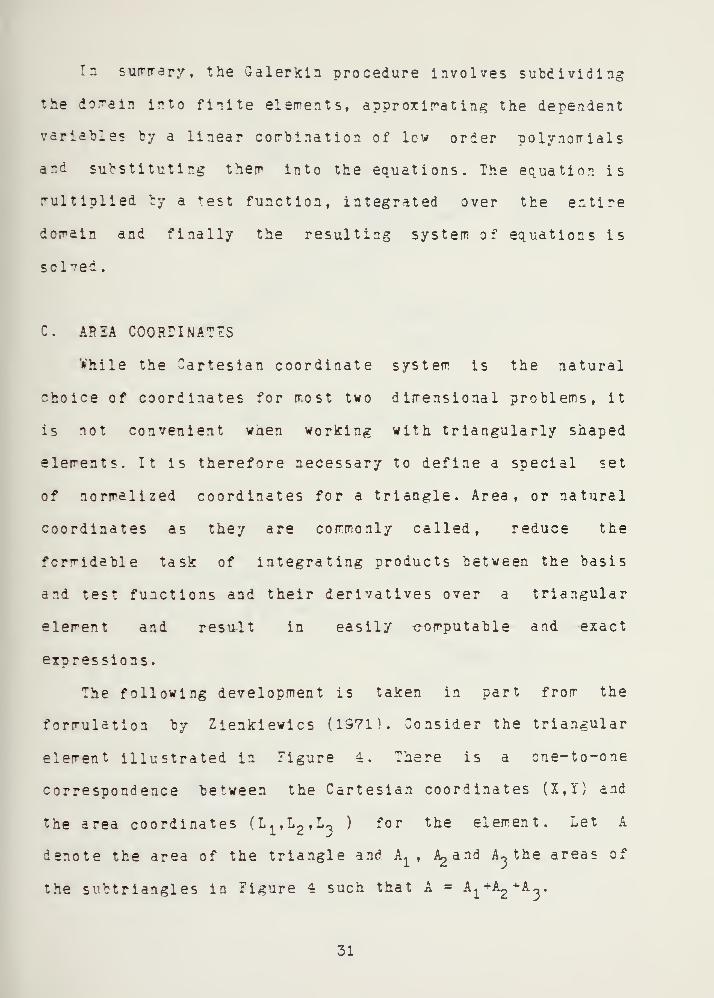
The following development is taken in part from the

formulation by Zienkiewics (1971). Consider the triangular

element illustrated in Figure 4. There is a one-to-one

correspondence between the Cartesian coordinates (X,Y) and

the area coordinates (L^Lg.L-a ) for the element. Let A

denote the area of the triangle and Aj_ , ^and A^ the areas of

the svbtriangles in Figure 4 such that A = A^+Ag+A,.

31

2 (X2,Y2 )

(0,1,0)

P(X,Y) or

Cartesian vs. area coordinates

YA

W 71

a3

" X2 " X

l'

W y2

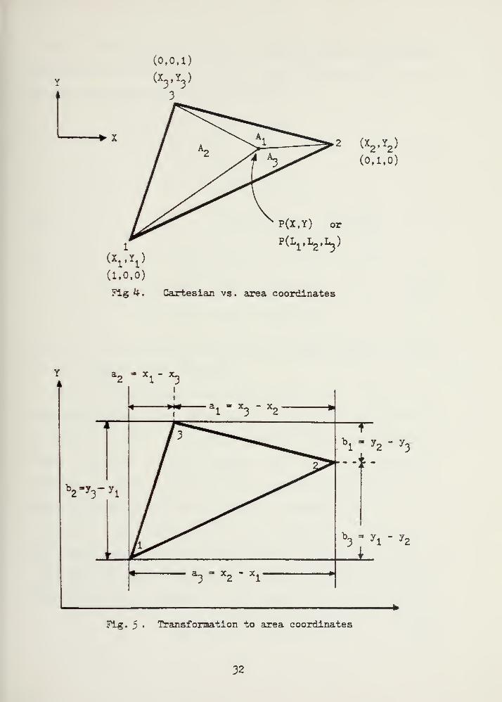
Fig. 5 • Transformation to area coordinates

32

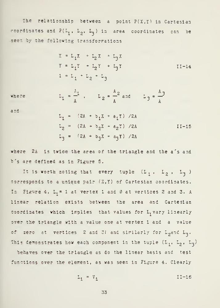
The relationship between a point P(X,I) in Cartesian

rcordinates and ?(L , L , L_ ) in area coordinates can be

seen by the following transformations

X = LjX + L2X * L-X

Y = L1Y + L^Y + L

3Y

1 = Ll

+ L2

+ L3

11-14

where .-* L- = - and* A

andL1

= f2A + b1X + a

1Y) /2A

L2

= (2A + b2X + a

2Y) /2A

L3

= '2A + b3X + a

3Y) /2A

11-15

where 2A is twice the area of the triangle and the a's and

b's are defined as in Figure 5.

It is worth noting that every tuple (L- , L2

, L-» )

corresponds to a unique pair fX,Y) of Cartesian coordinates.

In Figure 4, L- a 1 at vertex 1 and at vertices 2 and 3. A

linear relation exists between the area and Cartesian

coordinates which iirplies that values for L.vary linearly

over the triangle with a value one at vertex 1 and a value

of zero at vertices 2 and 3; and similarly for L2and L-

.

This demonstrates how each component in the tuple (L^, L2 , LJ

behaves over the triangle as do the linear basis and test

functions over the element, as was seen in Figure 4. Clearly

= 7. 11-16

33

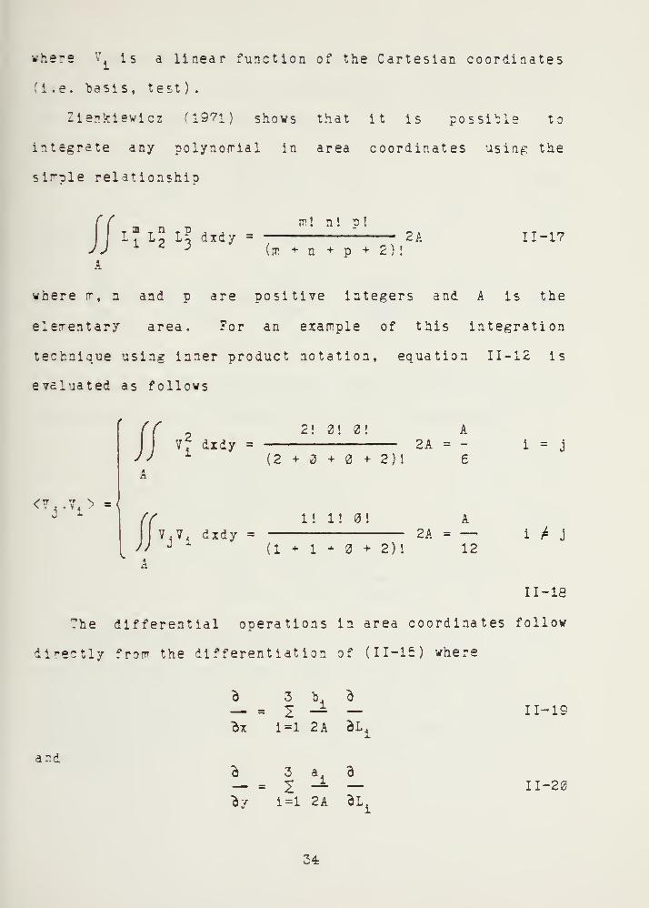
where V. is a linear function of the Cartesian coordinates

(i.e. "basis , test ) .

Zienkievicz (1971) shows that it is possible to

integrate any polynomial in area coordinates using the

sirole relationship

~ 1 ^2 ^3 dxd y=

m ! n ! o !

A( m. + n + p + 2 )

!

2A 11-17

where rrf a and p are positive integers and A is the

elementary area. For an example of this integration

technia.ue using inner product notation, equation 11-12 is

evaluated as follows

V^ didy =2! 0! 0!

2A = -

(2 + + 2)! 6

<vv-<f 1! 1! 0!

V.V, dxdy =J

(1 + 1 + +

A2A = —

2)! 12

i = J

i t J

11-18

The differential operations in area coordinates follow

directly from the differentiation of (11-15) where

ar.t

b 3 b. o

bx i=l 2A dL4

b 3 * a

'by i=l 2A bL.

11-19

11-20

34

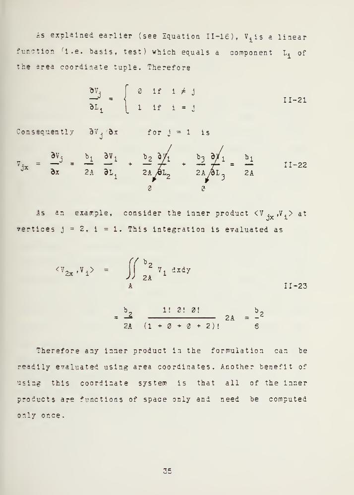
As explained earlier (see Equation 11-16), Viis a linear

function 'i.e. basis, test) which equals a component L1

of

the srea coordinate tuole. Therefore

5 =if 1 ^ j

1 if i =j

11-21

Consequently BV. dx

jx

dv.

dx

h. I! 1

2 A dl<

for j = 1 is

2A11-22

Is an exarrple, consider the inner product <V . ,v.> at

vertices j = 2, i = 1. This integration is evaluated as

<72x»V =(f b

y > 2A7

1±xdy

11-23

.!*1! 0!

2A = -

2A (1+0+0+2)! 6

Therefore any inner product in the formulation can be

readily evaluated using area coordinates. Another benefit of

using this coordinate system is that all of the inner

products are functions of space only and need be computed

only once.

i><j

III. SHALLOW WATIR ^Clil

The governing equations for this model are derived by

raking several simplifying assumptions on the primitive

equations of motion, whish then give the barctropic shallow

water equations. However, as mentioned previously, the

shallow water equations describe many significant features

of the large-scale motion of the atmosphere, and therefore

have been used in numerous experiments over the years.

The vcrticity-divergence form of the equations has

several advantages. Williams (1981) has shown that the

frecstrophic adjustment process is treated much better with

the vcrticity divergence formulation than with a direct

treatment of the primitive form of the shallow water

equations, such as was used by Kelley (1976). This

formulation also allows the~ velocity components and the

height to be carried at the same nodal points, whereas the

best scheme for the primitive form of the equations requires

staggering of the fields, as seen in Schoenstadt (1980). The

orticity divergence form of the equations is also

convenient for the application of semi-implicit

differencing, which saves considerable computer time.

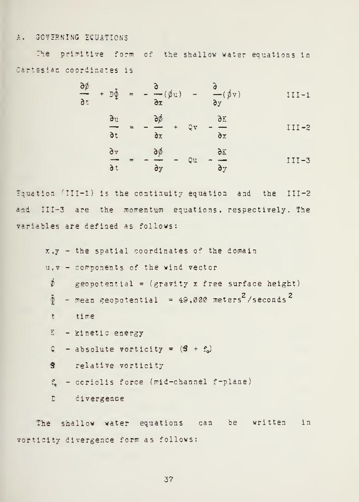
A. SOYIRNING EQUATIONS

The primitive form of the shallow water equations in

Tirtesiac coordinates is

dt dx dy

du 30 dK

dt ox dx

dt dy dy

III-l

III-2

III-3

equation (III-l) is the continuity equation and the III—2

ani 1 1 1-3 are the momentum equations, respectively. The

variables are defined as follows:

0,1

i

i

t

c

5

the spatial coordinates o* the domain

components of the wind vector

geopotential = (gravity x free surface height)

2 2mean geopotential = 49,000 meters /seconds

time

kinetic energy

absolute vorticity = (-9 + fj

relative vorticity

ccriolis force (mid-channel f -plane)

divergence

The shallow water equations can

vorticity divergence form as follows:

oe written in

3?

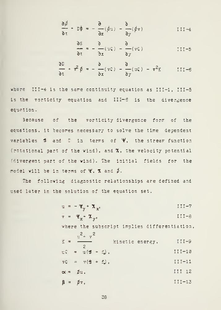
— + B(j) =

dt

dt

— T2^ =

&t

Ox(^u J

-

—(uQ)dx

d— (vC)dx

— (0v)By

— (vC)oy

d— (uQ)By

v2K

III-4

III-5

III-6

where III -4 is the sare continuity equation as III—1 , I I 1—5

is the vorticity equation and III— 6 is the divergence

equation .

3ecause of the vorticity divergence fortr of the

equations, it becomes necessary to solve the tirre dependent

variables "S and I in terms of 4/, the strearr function

(rotational part of the wind), and*X, the velocity potential

(divergent part of the wind). The initial fields for the

model will be in terms of ¥, TL and $,

The following diagnostic relationships are defined and

used later in the solution of the equation set.

u = "V*x> III-7

III-8

where the subscript implies differentiation,

2 2u * V

K = kinetic energy, I II—9

uC = u(* fj, 111-10

vC = v(S + fj , III-ll

Of = 0u, III 12

P = pv, I I 1-13

38

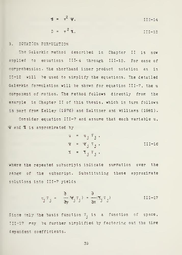
-8 - v2 V, 111-14

D - v2*. 111-15

3. IOUATION FORMULATION

The G-alerkin method described in Chapter II is now

applied to eauations III-4 through 111-15. For ease of

comprehension » the shorthand inner product notation as in

11-12 will be used to simplify the equations. The detailed

Galerkir. formulation will be shown for equation III-?, the u

component of motion. The method follows directly from the

example in Chapter II of this thesis, which in turn follows

in part from £elley (1976) and Ealtiner and Williams (1981).

Consider equation I I 1-7 and assume that each variable u,

^ and 1 is approximated by

- - W* = ¥. v. , in-ie

where the repeated subscripts indicate summation over the

range of the subscript. Substituting these approximate

solutions into 1 1 1-7 yields

»T =* ~^J.) + —(* 7.) 1 1 1-17

Since only the basis function 7. is a function of space,

TII-17 may be further simplified by factoring out the time

dependent coefficients.

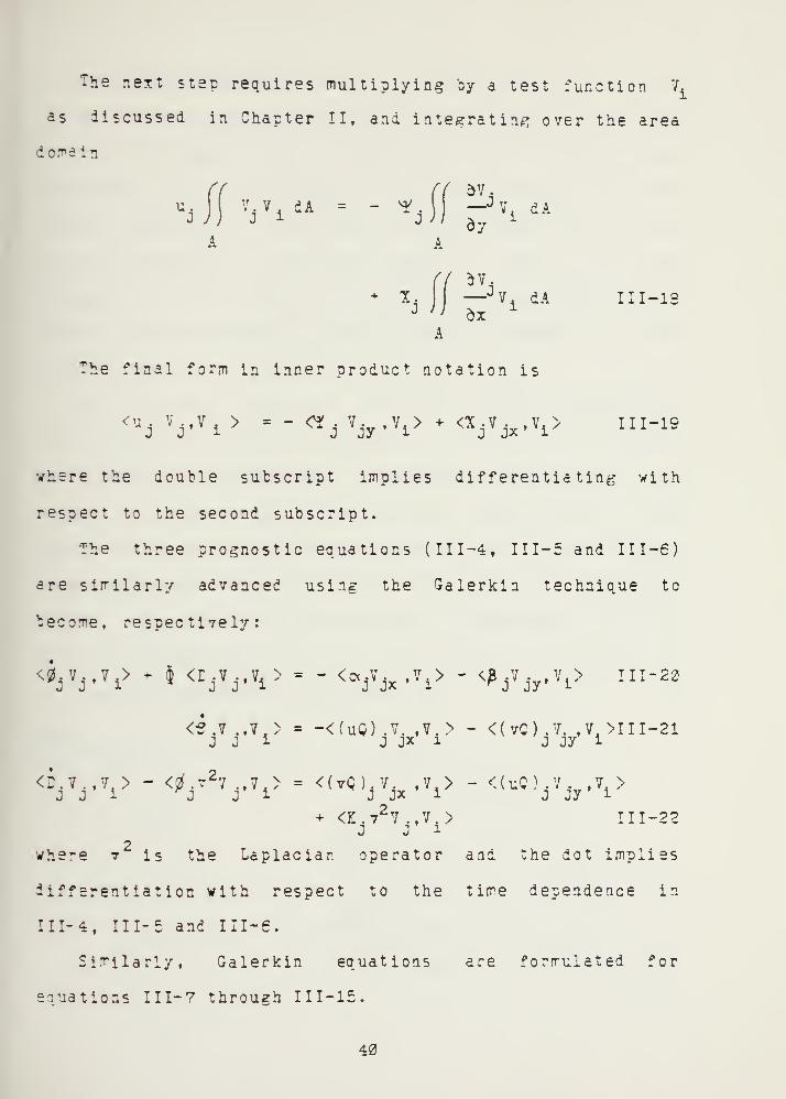
The next step requires multiplying by a test function V.

as discussed in Chapter II, and integrating over the area

domain

( av.—J V, dAay

iv. v, dA = - ¥

A

J J

(( 5V.—JV, dA

dxx

III-1S

'he final form in inner product notation is

<uj

Tj- T i>

= " «J 7JT'

T1> + <V±C' Ti> nI - 1SJ JX

where the double subscript implies differentiating with

respect to the second subscript.

The three prognostic equations (III-4, III—5 and III-6)

are similarly advanced using the Galerkin technique to

become, respectively:

<Vr Ti>

+ l <rjW =- <^vjx« v i> ' <*jTjrV IXI " 20

<tjfj.fi> = -<(ug).V vi>-<(vc).V v

i>in-2i

,2,<r.V. f 7, > - <0.V*V .,7,> = <(vQ).V. ,V,> - <(uC) .V . ,T, >J J i *J J i J Jx i J jy i

+ <£.v2 7 .,V. >J J i

TT T-??

where v is the Laplacian operator and the dot implies

differentiation with respect to the time dependence in

III-4, III- 5 and III-6.

Similarly, Galerkin equations are formulated for

equations III-7 through 1 11-15

.

40

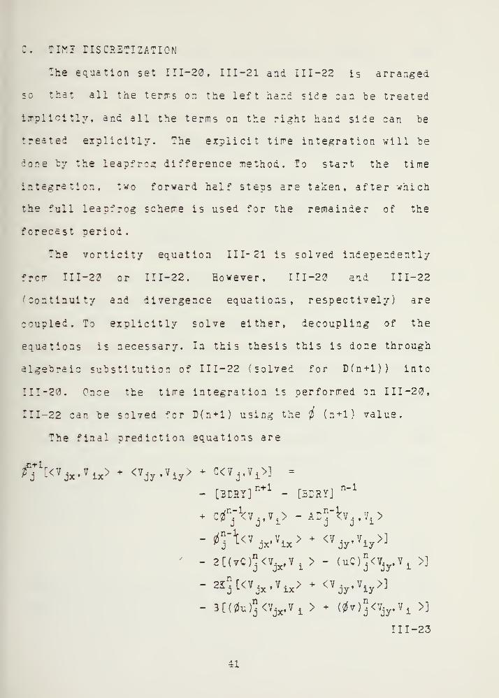
C. TIMZ riSCP.ETIZATION

The equation set 1 1 1-20, 111-21 and 111-22 is arranged

so that all the tern's on the left hand side can "be treated

Implicitly, and all the terms on the right hand side can he

treated explicitly. The explicit time integration will be

done by the leapfrog difference method. To start the time

integration, two forward half steps are taken, after which

the full leapfrog scheme is used for the remainder of the

forecast period.

The vorticity equation III- 21 is solved independently

frcr 111-20 or 111-22. However, 111-20 and 111-22

'continuity and divergence equations, respectively) are

coupled. To explicitly solve either, decoupling of the

equations is necessary. In this thesis this is done through

algebraic substitution of II 1-22 (solved for D(n+1)) into

IIT-20. Once the time integration is performed on 111-20,

111-22 can he solved 'or E(n+1) using the i (n+1) value.

The final prediction equations are

- [3EHT]n+1

- [BEEYJ°~1

" 2E j[< T jx- V ix>+ < V jy Viy>]

111-23

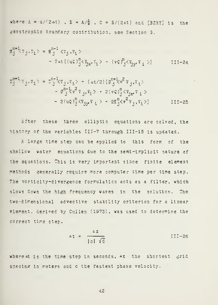
whe-e A = 4/(2*t) f E = A/J f C = B/(2*t) and [BERY] is the

geostrcphic boundary contribution, see Section 3.

.n+1v?j.f1 >

n-1*j <V

j,Vi >

J3(^Wi >] I I 1-24

rj

T'j' 7i'- D

n

J1<7jf 7i > - (At/2)[0

n

j

+1<v

2v

j,V

i>

* ^S'V * 2(TQ)3<fja,? 1 >

111-25

After these three elliptic equations are solved, the

history of the variables I I 1-7 through 111-15 is updated.

A large time step can he applied to this forrr of the

shallow water equations due to the semi-implicit nature of

the equations, -his is very important since finite element

methods generally require more computer time per time step.

The vcrticity-divergence formulation acts as a filter, which

slows down the high frequency waves in the solution. The

two-dimensional advective stability criterion for a linear

element, derived by Cullen (1973), was used to determine the

correct time step,

4 x

^t =

Id i/e

111-26

whereat is the time step in seconds, ax the shortest grid

spacing in meters and c the fastest phase velocity.

42

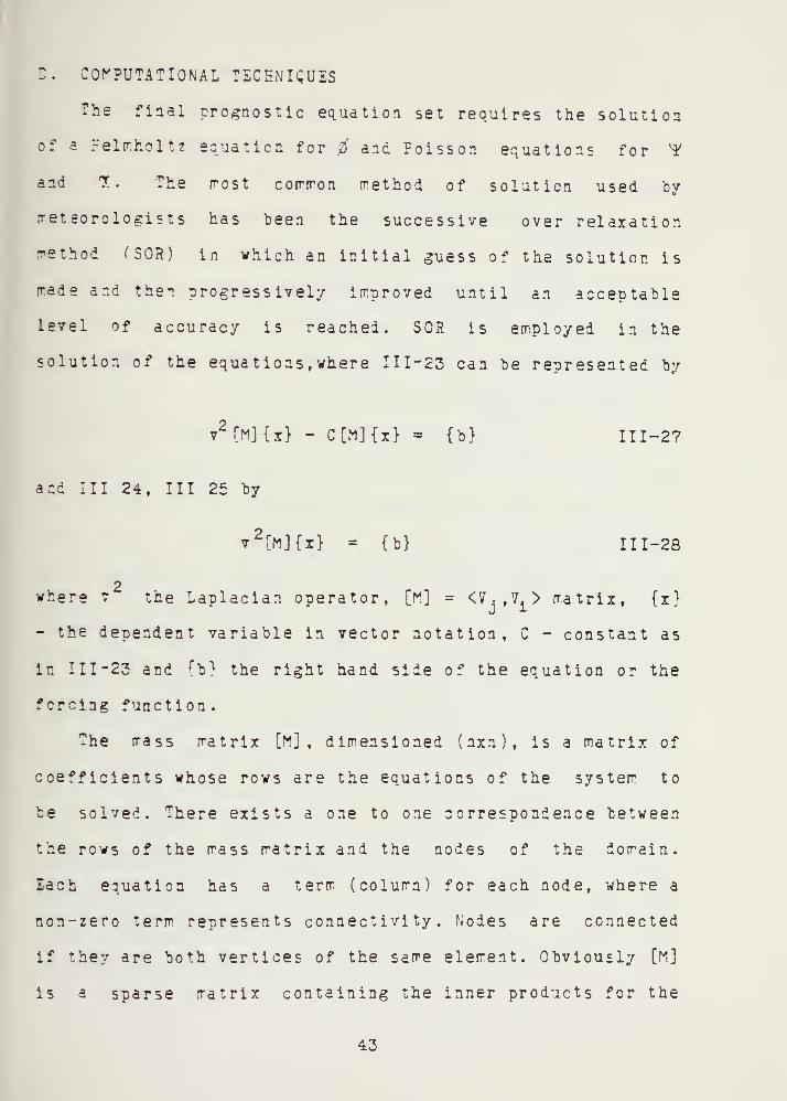
D. COMPUTATIONAL TECHNIQUES

The final prognostic equation set requires the solution

of a Felmholtz equation for $ and Poisson equations for ¥

and J.. The rrost common method of solution used by

meteorologists has been the successive over relaxation

method (SOH) in which an initial guess of the solution is

trade and then progressively improved until an acceptable

level of accuracy is reached. SOH is employed in the

solution of the equations, where 111-23 can be represented by

v2[M]{x} - C[M]{x} * {b} 111-27

and III 24, III 25 by

v2[M]{x} = {b} 1 1 1-28

2where v the Laplacian operator, [M] = <V-,V.> matrix, {x}

- the dependent variable in vector notation, C - constant as

in III -23 and {b} the right hand side of the equation or the

forcing function.

The mass matrix [M] , dimensioned (nxn), is a matrix of

coefficients whose rows are the equations of the system to

be solved. There exists a one to one correspondence between

the rows of the mass matrix and the nodes of the domain.

Each equation has a term (column) for each node, where a

non-zero term represents connectivity. Nodes are connected

if they are both vertices of the same element. Obviously [M]

is a sparse matrix containing the inner products for the

43

left hand side. Chapter 4 of this thesis will describe the

matrix compaction procedure.

The forcing function {b}, dimensioned (nil), involves

only variables at the current time step and is easily

computed using four very versatile subroutines described in

detail in the next chapter.

The initial guess to start SOR is the previous time step

solution. An average of 30 passes per equation are needed

for each time step. The solution is considered to have

converged to its final value when the residual for each node

has beer, reduced to some acceptably small value.

The diagnostic equations III-7 through 111-15 must also

be solved every time step. Eowever, the same technique is

not used for these equations. Dr. V .J.P. Cullen suggested an

ur.de- relaxation scheme for which three passes over the

domain should produce a solution of acceptable accuracy,

since the coefficient matrix is so strongly diagonally

dominant. .

yass lumping of the coefficient matrix is used for

the first guess. This technique requires replacing the mass

mat-ix [«] by the identity matrix [I] . A first guess of this

type i? *ble to describe most of the large scale features,

whi~h in turn reduces the number of iterative passes ever

the field. Successive passes converge to solutions which

describe smaller scale motion, approximately to the same

order of magnitude as introduced by computational error, so

that further iterations are not needed.

44

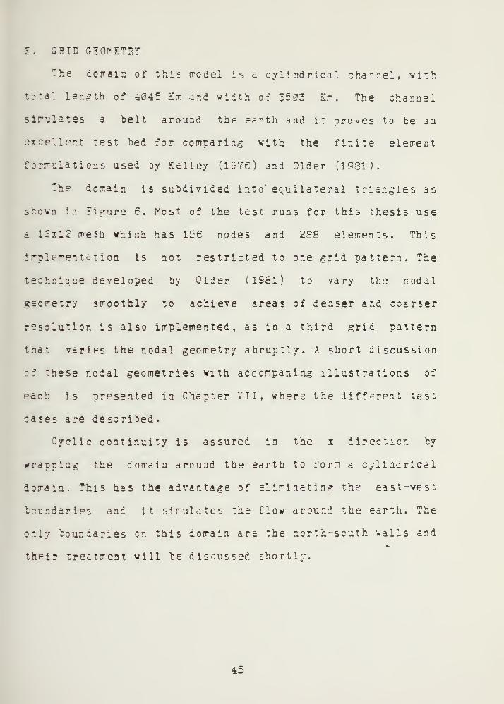
I. GRID GIOPSTRT

The dor-air. of this trodel is a cylindrical channel, with

total length of 4245 Km and width of 3503 Km. The channel

simulates a belt around the earth and it proves to be an

excellent test bed for comparing with the finite element

formulations used by Selley (1576) and Older (1981).

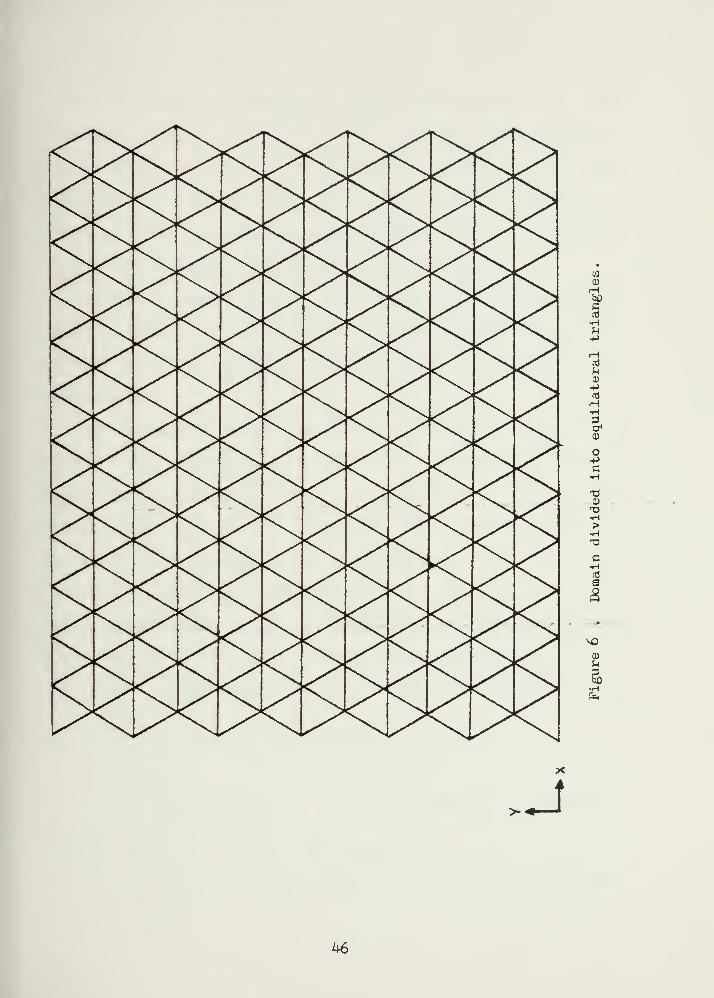
The domain is subdivided into' equilateral triangles as

shown in Figure 6. Post of the test runs for this thesis use

a 12x12 mesh which has 156 nodes and 289 elements. This

implementation is not restricted to one grid pattern. The

technique developed by Older (1931) to vary the nodal

geometry smoothly to achieve areas of denser and coarser

resolution is also implemented, as in a third grid pattern

that varies the nodal geometry abruptly. A short discussion

of these nodal geometries with accompaning illustrations of

each is presented in Chapter VII, where the different test

cases are described.

Cyclic continuity is assured in the x direction by

wrapping the domain around the earth to form a cylindrical

domain. This has the advantage of eliminating the east-west

boundaries and it simulates the flow around the earth. The

only boundaries en this domain are the north-south walls and

their treatment will be discussed shortly.

45

w

G

•H

a)

Uo

-t->

oj

3

o

g

-a0)

T3

>•HT3

C

o3

e5

•H

J

46

F. INITIAL CONDITIONS

As mentioned previously, the reformulation of the

governing equations into the vorticity-divergence

shallow water equation set requires solving the tirre

dependent variables in terms of the stream function and

velocity potential. The continuity equation is not altered,

so that its solution is expressed in terms of i.

For the basic testing of the model's performance, simple

analytic sinusoidal initial conditions are used to insure

the most accurate analysis possible and to simplify the

comparisons .

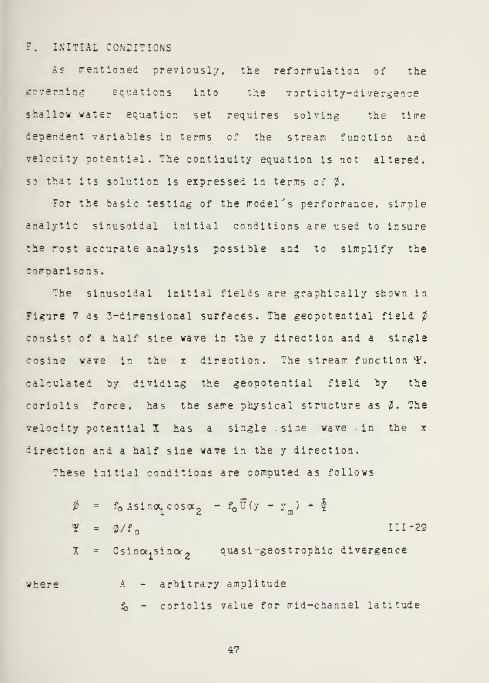
The sinusoidal initial fields are graphically shown in

Figure 7 as 3-dimensional surfaces. The geopotential field

consist of a half sine wave in the y direction and a single

cosine wave in the x direction. The stream function ¥,

calculated by dividing the geopotential field by the

coriolis force, has the same physical structure as 0. The

velocity potential 1 has a single sine wave in the x

direction and a half sine wave in the y direction.

These initial conditions are computed as follows

= fQ Asinoc1cosoc

2- f U(y - y^) - $

¥ = 0/f o111-29

1 = CsinocjSinop quasi-geostrophic divergence

where A - arbitrary amplitude

& - coriolis value for mid-channel latitude

47

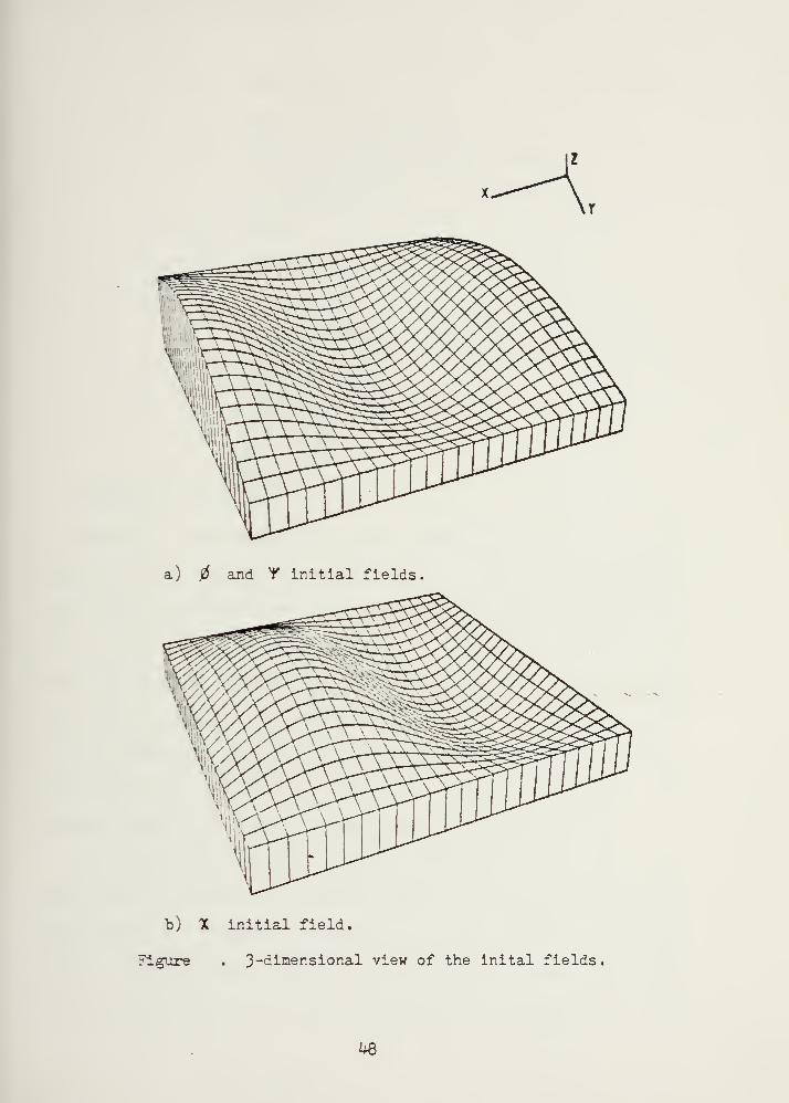
a) and Y initial fields.

b) X initial field.

Figure . 3~G-imer-sional view of the inital fields.

48

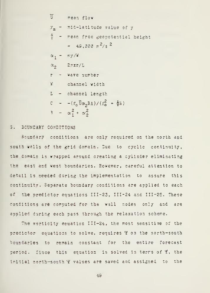
3

mean flow

m id-la t i tude value of y

| - rear, free geopotential height

= 49,200 m2/s

2

2^xr/L

wave number

channel width

*i-

*2

r

V

L - channel length

- -(f Uoc?BA)/(f§ + $3)

*1 + *2

3. 5CUNEARY CONDITIONS

3oundary conditions are only required on the north and

south walls of the grid domain. Eue to cyclic continuity,

the domain is wrapped around creating a cylinder eliminating

the east and west boundaries. However, careful attention to

detail is needed during the implementation to assure this

continuity. Separate boundary conditions are applied to each

of the predictor equations 111-23, 111-24 and 111-25. These

conditions are computed for the wall nodes only and are

applied during each pass through the relaxation scheme.

The vorticity eauation 111-24, the most sensitive of the

predictor equations to solve, requires ^ on the north-south

boundaries to remain constant for the entire forecast

period. Since this equation is solved in terms of ¥, the

Initial north-south ¥ values are saved and assigned to the

49

"boundary points after each pass through the relaxation

subroutine.

-he oroper boundary condition for the divergence

equation III —25 would be dX/dn = C. However, for the purpose

of this study, there is more interest in the sinusoidal

variation in the y direction and not in the region of the

walls. Therefore I = 2 is appropriate.

The continuity equation 111-23, the most complex

predictor equation, requires that there be no mass flux

through the north-south walls. The geostrophic boundary

condition

— = -uf 111-30dy

is aoplied to the north south boundary nodes for the terms

[BEET] in equation I 11-23 . Integrating the inner product

<£ • V.,V. > by Darts produces the boundary terms

If v2 (0.V )V. dxdy = f / * • (* $ .V. ) V .dxdy

yx J J yx J J

= \[ [v.(Viv(^V

j)) - v^V^-vV^ dxdy

= i V. v(0 .7. )-S ir - // W. .v(^.V, ) dxdy

= r3ERTl - ^[<v jx .v ix > - <Vjy

.V ly >] 111-31

where n is a unit vector normal to the domain and dr is the

differential distance along the path of integration on the

perimeter of the domain.

52

"he geostrophic boundary condition 111-38 is substituted

into the contour integral in equation 1 1 1-31 and put into

laleriir forrr, in the sare way as in the one-dimensional

advective equation in Chapter II. The resulting term is

derived as follows

i V.v'0.7.).n dr = & —(#.V.) V, dxoy

v*x(u . . + 2u. u. . ), 111-32

3 J+l J J-l i

Equation 1 1 1-32 appears twice in the continuity equation

III 23, for *ime levels (n+1) and (n-1). All values of u are

known "or time (n-1), since they are saved from the previous

calculations. Fowever, u(n+l) has not been computed. To

solve for u(n+l), both¥(n+l) and T(n+1) are needed, ^(n+l)

is solved first from the vorticity equation. 1(n+l) needs

0(?»+l) as part of its solution and 0(n+l) needs u(n+l) in

its solution. To avoid this problem, it is assumed that

X(b+1) has a negligible contribution to the solution of

ufn+1) and only ¥( n*l ) is used.

51

iv . gcrruTiR ieplimintation

The formulation and general theory of the finite element

method was presented in the previous chapters. The objective

In this chapter is to discuss sere Important computational

aspects pertaining to the implementation of the finite

element prediction system.

The nain advantage that the finite element method has

over other prediction techniques is its generality.

Conceptually, it seems possible by using many elements, to

approximate virtually any surface with complex boundaries

iz 1! initial conditions to such a degree that an accurate

solution can be obtained. In practice, however, obvious

engineering limitations arise, a most important one being

the cost of the computation. As the number of elements is

increased, a larger amount of computer time is required for

a forecast. Furthermore, the limitations of the program and

the computer may prevent the use of a large number of

elements. These limitations may be due to the computer speed

and stcrage availability, or round-off errors propagated in

the computations because of finite precision arithmetic.

Also, the malfunction of a hardware component, if the

prediction is carried out using many computer hours to

execute, can be a serious problem. It is therefore desirable

to use efficient finite element programs.

KO

The effectiveness of a program depends essentially or.

the following factors. Firstly, the use of efficient finite

element techniques is important. Secondly, efficient

programming methods and sophisticated use of the available

computer hardware and software are important. The third very

iirportfint aspect in the development of a finite element

oro^ram is the use of appropriate numerical techniques.

The vcrtici ty-divergence model described in the previous

chapter is implemented on the 13m" 3333 computer located at

the Naval Postgraduate School. Some notable features of its

architecture are the three trillion bytes of virtual mass

storage, of which eight mega bytes are available to each

user, and the c7 nanosecond machine cycle time. The model is

executed rostly using a 12x12 element domain requiring 4201c

bytes of storage and 30 seconds of CPU time to execute.

Irceeding execution time and/or available storage is not a

problem, in fact the system allowed a lot of flexibility

during the implementation phase of the model.

The source code is written using FORTRAN IV and compiled

on an optimizing Fortran H compiler. Appendix A contains the

source cede listing, which is divided into five subdivisions

delineating the logical structure of the program.

A. PROGRAM ARCEIT£CTURZ

Program features incorporated in the model are:

1) Modularity. With only a few exceptions, each

module is limited to one page of FORTRAN code. This makes it

53

easier to comprehend the program. Zach module performs only

o-^e task. For example, subroutine CONTIC computes the value

jf the forcing terms for the continuity equation. likewise

there is also one module for the divergence and vcrticity

equations. To implement a new set of equations, only these

modules would have to be altered.

"asily controllable switches. Switches may be set

to either print, plot or tabulate harmonic analysis data for

most of the available fields. The ability to display

intermediate results allows each portion of the algorithm to

be monitored for computational adjustments. This also makes

it easier for unfamiliar users to become acquinated with the

computational model.

3 ^ Forcing term subroutines. In previous

irpiementaticns • each forcing term was calculated by a

special subroutine. In this implementation, the calculations

are accomplished by general purpose routines which simplify

the implementation of the complex prognostic equations:. Hits;

allows implementation of different equation sets (i.e.

^aroclinic y odel) over the same domain with minimal effort.

4< T cementation . Zach variable is defined by a

short phrase 'Appendix A, A.). The function of each module

is described in an introductory paragraph. Shared data is

placed in named common blocks and identified with each

subroutine which uses them. A subroutine index is given.

1 . "air, Program

The main program is short, calling only six modules

which reflect the basic sequential flow of the model. It

starts with initialization of all model parameters (i.e.

model options, domain, finite element arrays, inner

products). It then initializes the input fields (i.e.

secpctential heights, stream function and velocity

potential) and is followed by initialization of all

remaining dependent variables. At this time the model is

totally initialized and time integration begins. As

mentioned previously two techniques are employed for time

integration, each having its own module. Upon completion of

the last forecast, the program terminates.

Arrays are the only data structures used and are

grouped using 19 different common blocks. Several arrays are

use! as static link lists, as described in detail later,

which simplified the algorithms. The common block format has

the advantage of reducing the overall execution time of the

program. Most of the arguments passed during a call to a

subroutine are contained in conmon. This requires less time

to execute since no parameter passing is required for the

arguments. Another benefit of this format is that the code

becomes less cumbersome and more readable. Each variable and

array is defined in the first subsection of Appendix A along

with a oage index for the subroutines.

2. Initialisation Phase

Appendix A, Section C contains all the subroutines

used during the initialization phase of the program. Frorr

the user point of view, the most important suoroutine is

INI-S3, the first subroutine called, which contains all the

global variables that control the different options

available per run. This is the only subroutine that is

changed to run the different experiments, assuming that no

new computational technique is introduced. The selection of

options ere:

1) - channel location - the channel may be

shifted north or south by presetting the

north/south latitude limits in INITG3.

2) - variable geometry - the node positions may

be grouped for more dense node patterns to

yield higher resolution. Two variables HI

and H2 set the ratio used to vary the

spacing -along the x .and y. axes,

respectively.

3) - initial field wave length and amplitude can

be altered to produce various effects.

4) change the initial mean flow.

5) - diffusion can be entered for any of the

three prognostic equations.

6) - maximum length of forecast period may be

changed and a print, plot or harmonic

c p.

analysis of any dependent variable may be

requested for any tire interval.

Or.ce the experiment is determined, the options

listed above are set. The program is ready to be executed.

The largest part of the initialization phase

consists of establishing the domain and producing ail the

finite elerent computational vectors that remain constant

throughout the experiment.

"he first several steps in setting up the domain are

concerned with indexing. Subroutine COF.RES is called first,

where all the nodes (grid points) and elements (triangular

areas' 1 are numbered consecutively starting at the southwest

corner of the domain and moving eastward across each row or

latitude. lor earch element, a record- -of all of its nodes

(ertlces) *re stored in array ELMENT (M,2), where M is the

total number of elements. To facilitate the inner product

evaluation later, a local numbering system is required for

each element. That is, for each element, its nodes are

stored counterclockwise in a positive sense. The first node

however, is arbitrary.

With the domain divided and numbered, a connectivity

list ( the correspondence between each node and the neighbor

nodes) is constructed for each node by subroutine CORRIL.

lach node is adjacent to four or six other nodes depending

on whether it is a boundary or interior node, respectively.

These adjacent nodes, plus itself, make up the connectivity

57

list for one node. The connectivity lists are then

concatenated sequentially starting with the first nodes

connectivity list into the vector NAME (NN), where NN is the

sur of the nodes in each connectivity list. (i.e. for a

12x12 dorain with 156 nodes, and equilateral elements NN =

1044). 3or the first tiire during the initialization phase,

special attention is given to cyclic continuity. As

discussed earlier, cyclic continuity is the joining of the

east and west "boundaries to create a cylindrical channel.

The connectivity list for these east/west boundary nodes

must be complete to insure proper continuity for the

calculations later.

The connectivity vector NAM is frequently used

during most computations. Two utility vectors ISTART

(containing the starting location in NAM for a particular

node' and MUM (containing the number of nodes in its

connectivity list) are used to locate and indei through the

vector NAMI, as will be seen shortly. This same technique is

used to index through the coefficient matrices and used

during most of the node interaction computations.

The physical properties of the channel are

calculated next in subroutine CHANAL. Here the north and

south latitude boundaries, which were pre-set in INITG£ by

the user, are used to compute the grid spacing along the x

and y axis. Since this channel simulates a belt around the

earth, the magnitudes of both LIITAX and DELTAY (meters) are

£3

proportional to the width of the channel divided by the

number of ,?rid points in the y axis.

The Cartesian coordinates for each node are computed

by subroutine LCCATI using the DILTAX and EILTAY calculated

in CEANAL. If the option to use varying grid geometry is

i-sired, subroutine TRANS transforms the grid geometry.

TRANS also computes the corresponding new Cartesian

coordinate values for each prid point and calculates the

minimum E5ITAX and IELTAY within the domain. When the

secmet-y is changed to create a smaller DELTAX or DELTA!,

the two dimensional advective stability criteria is also

charged. A new time step DT has to be computed using

equation II 1-26. Since TRANS transforms the geometry, it

also computes the new CT

.

Another transformation is required as discussed in

Chapter II. The transformation from Cartesian coordinates to

area coordinates is needed to perform the area integration

of the inner products. Sub-routine AREA computes these

transformations exactly as outlined in Chapter II, Section

C. Again cyclic continuity is very important and special

care is needed to insure proper transformation.

Following the area transformation is the computation

of all the inner products that are required to solve the

equations. The advantage of using area coordinates is that

the inner products (function of space coordinates only) are

computed and stored once and used repeatedly without

53

recalculation- Subroutine INN2P. computes and stores these

products using the formulas derived In Chapter II.

The 3oefficlent matrix, dimensioned NxN , where N is

the total number of nodes, is a matrix of coefficients whose

rows are the equations of the system to he solved. As

discussed In the computational technique section, the

members of this sparse matrix are the inner products for the

left hand sides of the equations. Three coefficient matrices

are used in the solution of the equations. The diagnostic

equations (III-? through 111-15) use a coefficient matrix

with the inner product <V ,,L > which is constructed by

subroutine AMTHXl and stored in compacted form in vector

GfNN) by subroutine ASEMBL. Eowever, when solving the

prognostic equations, these coefficient matrices have a DT

ftlire step in seconds) term, so that these matrices are not

assembled until the time integration begins. The vorticity

and divergence equations (111-24,111-25) use the coefficient

matrix H(N'N) with inner products < vjx

.? lx > + <vjy*\y> in

solving the ?oisson equations for the stream function and

velocity potential, respectively. The continuity equation

[111-23) uses a combination of inner products in its

coefficient matrix J(N'N) as follows

jx» v ix^ V¥jy *

v iy'J(At)

<vj,v

i >iv-i

60

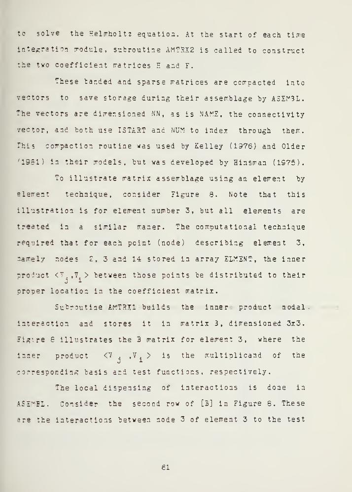
to solve the Helirholtz equation. At the start of each tirre

Integration module, subroutine AMTHX2 is called to construct

the two coefficient matrices E and F.

These banded and sparse rratrices are ccrrpacted into

vectors to save storage during their assemblage by ASEM3L.

The vectors are dimensioned NN, as is NAME, the connectivity

vector, and both use ISTART and NUM to index through them.

This compaction routine was used by Kelley (1976) and Older

'1981) in their models, but was developed by Hinsman (1975).

To illustrate matrix assemblage using an element by

element technique, consider Figure 8. Note that this

illustration is for element number 3, but all elements are

treated in a similar maner. The computational technique

required that for each point (node) describing element 3,

namely nodes Z, 3 and 14 stored in array ELMENT, the inner

nro-uct <TT .,7 J

> between those points be distributed to theirJ i

proper location in the coefficient matrix.

Subroutine AMTRI1 builds the inner, product nodal

interaction and stores it in matrix 3, dimensioned 3x3.

Figure 6 illustrates the 3 matrix for element 3, where the

inner product <V . ,V.> is the multiplicand of the

corresponding basis and test functions, respectively.

The local dispensing of interactions is done in

ASZ VBL. Consider the second row of [3] in Figure 8. These

are the interactions between node 3 of element 3 to the test

61

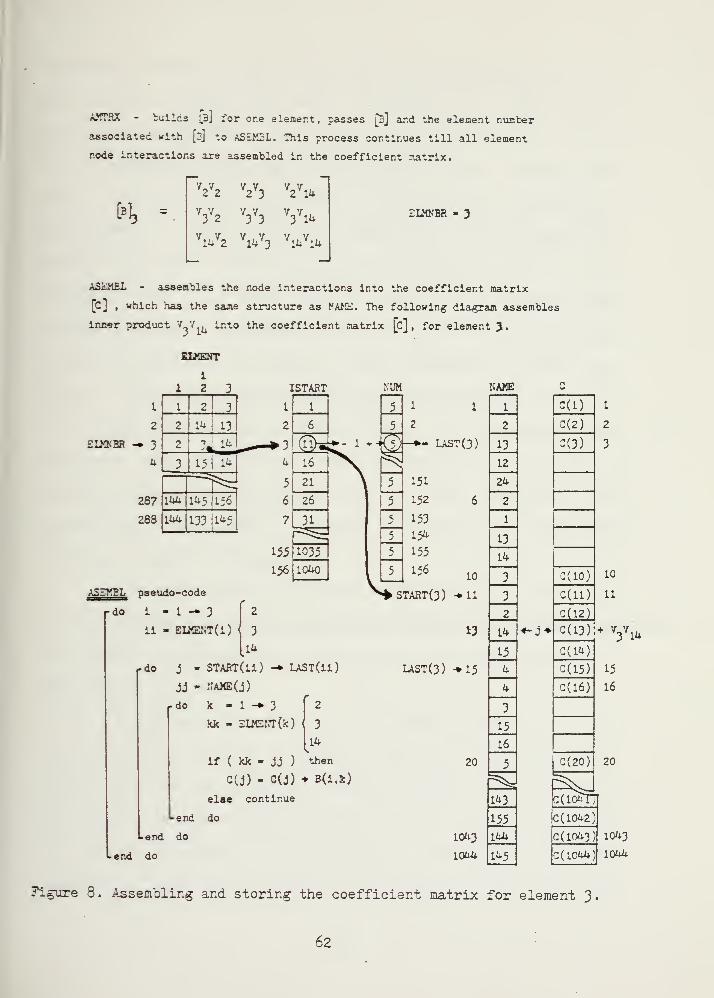
AMTRX - builds J3J ^OT one element, passes [3] and the element number

associated with [2] to ASEK3L. This process continues till all element

node interactions are assembled in the coefficient matrix.

H,

V2

V3V2

V3

V3V3

V14

V2

V1V3

Vl4

Yl*V14V14

ELMJ-'BR

ASEMBL - assembles the node interactions into the coefficient matrix

[Cj , which has the same structure as HAKE. The following diagram assembles

inner product '•jj. into the coefficient matrix [c] , for element J.

EIKENT

1

1

2 3

1 1 2 3

2 2 14 13

ZLKNBR -» 3 2 ill*]

4 3 15 1

1^

"rH287 144 145 |156

288 Vtk 133 1*5

ISTART

1 1

2 6

3 ©*-^

4 16^

5 21

6 26

7 31

155 1035

156 1040

KUM

5 12

SH

ASZTBL pseudo-code

-do i - 1 -• 3 2

11 - SLMENT(l) 1 3

u-do j - START(ii) -* LAST(li)

jj - NAME(j)

-do k • l-»3 2

kk - 2LMEKT(k) 1 3

if ( kk - jj )

14

then

C(J) - G(j) * B<i,k)

else continue

L end do

-end do

-end do

sg

^s-

5 151

5 152

5 153

5 154

5 155

5 156

LAST (3)

NAME

1 1

2

LAST (3) 13

12

24

6 2

1

13

14

10 3

3) -m 3

2

13 14

15

3) *15 4

4

3

15

16

20 5

143

155

1043 144

1044 145

C(l)

:(z)

2(3:

:(io)

c(n)

liizi

10

11

c(i3):+ y^:(14)

c(l5)

c(l6)

0(20:

15

16

G(1042)

C(1043)

C(1C44)

20

1043

1044

Figure 8. Assembling and storing the coefficient matrix for element 3.

62

functions. AS1KBI locates nodes 3's connectivity list in

NAM! using ISTARI and NUM. In Figure 8, this list is

delineated ty START(3) and LAST(3). Now ASEMBL steps through

the connectivity list for three iterations. Turing each

pass. ASI.V 3L is searching for one of the three node numbers

for element 3. When a match is found with one of element 3's

nodes 'i.e. 2,3 or 14) and node 3's connectivity list (i.e.

3,2,14,15 or 4) the proper position, to which this

interaction is to he added has been found in the coefficient

matrix. Since MAPE and vector C, the compacted coefficient

rat Mi, are dimensioned identically, the same pointer (i.e.

J in Figure 3) is used to index through both arrays. This

procedure is repeated for all elements in the domain to

assemble the coefficient matrix of the equations. The

pseudo-code for ASEMBL is shewn in Figure 8 to facilitate

stepping through this exarrple.

The domain and all finite element work: vectors are

initialized at this point. Subroutine ER-MS3T is called- .later

to compute interpolation points for the harmonic analysis

subroutines.

The last phase of the initialization process is the

initialization of the dependent variables. The three input

fields geopotentlal heights, stream function and velocity

potential are computed in subroutine IC using the equation

set II 1-30 . However, the variables calculated from the

diagnostic equations have to be computed using the input

fields. These varieties are used during each tiire step while

solving the prognostic equations.

The diagnostic equations are solved in subroutine

DIPTAB, first during the initialization phase and later

during the time integration phase. Each diagnostic equation

calls its own module to compute the value of the forcing

function and stores the computed values in the vector RES.

These equations all use the same coefficient matrix when

solving the diagnostic equations. Subroutine SOLVER is

sufficiently genereal to solve each equation. SOLVER uses

vector RES and coefficient matrix G to under-relax towards

the solution. As mentioned previously, the coefficient

matrix is strongly diagonally dominant so that three passes

over the domain are sufficient. At the end of rEFVAR, output

is generated depending on what print, plct, or harmonic

analysis controls were preset.

This completes the initialization pnase of the model

and the program, for the forecast phase will he described

next

.

2 . Forecast Phase

The forecast phase is accomplished in two steps. The

first time step is made using two half steps by subroutine

r*£TZNO. Eere the prognostic coefficient matrices are

constructed using half the ET value by calling AMTRX2.

Ar"TFX~ uses the same computational technique to construct

the ccefficient matrices as described for AMTRX1

.

64

lach of the prognostic eauations 111-23, 111-24 and

111-25 calls its own subroutine (CONTIC, VORTEQ and TIVEC

respectively' to compute all the terms on the right hand

side, which are stored in the vector HHS. After computations

for RES are completed, subroutine RELAX solves the equations

by over-relaxation as described in the computational

technique in Chapter 3. Once the solutions for the (n+1)

time step are completed, DEPAB is called to update the

variables from the diagnostic equations. Two oasses through

rtATZNO advances the solution fields one time step.

The remainder of the forecast period is integrated

using the leapfrog scheme. Subroutine L2APFR performs this

integration using the identical format as vATZNO, except

that IT equals two DT. At preset times as specified in

INITG5, the different fields are saved for printing. This

process continues until the final forecast time is reached.

B. UTILITY YOTULZS

Ir.ce the equation formulation is completed, as in

Chapter III, all the inner products and types of

integrations are inown. Versatile modules can oe written to

per^crm these computations. Consider a term of general form

<^A . V . ,V . > where i is the node about which the term is

evaluated and the j's are the nodes connected to node i, or

the surrounding nodes. The inner product values <V.,V > are

already computed and stored for all the nodes, during the

Initialization nhase of the model.

65

-he regaining computation to complete trie evaluation of

this term is the mult iplicat ion of the scalar coefficient of

A it node 1 with the corresponding inner product <V.,V. > for

node «. This requires indexing through node i 's connectivity

list stored in vector NAME, and for each node in the list

irnltiply and total the products. The cumulative sum of these

multiplications is assigned as node i 's contribution for

this term. Subroutine TER V 3 performs this exact computation.

All that is passed to 7ERM3 is the scalar field A and the

sign of the inner product, TEBM3 then computes the

contribution for each node in the domain and accumulates it

in the wcric vector RES.

Three other utility modules are; TERM1, which computes

the first scalar multiplication for triple inner products

'i.e. /Aj Vj3k Vk ,Vi >) . The product <V.V

k,V£

f is again already

computed and stored by subroutine INNER. TERM1 computes <\ ?.

V k ,7 i > and constructs a compacted vector similar to the

coefficient matrices. This reduces the effort of multiplying

the second scalar to a TERf3 computation. TZRP2 computes

node interaction of the following type <Aj Vjxt 7^x> , where both

the basis and the test functions are derivatives. Lastly,

subroutine TIRK4 computes node interaction for terms as <A.V.3 Jx

,v\ , where only the basis function is a derivative.

When examining the right hand side of the equation sets

111-23, 111-24 and 111-25, it is obvious this implementation

is a subscripting nightmare; however, the use of the utility

66

modules TESM1, TERM2 , TERM3 and TERM4 simplifies the

irplementation to only determining what order to call the

utility modules. Examination of subroutines CONTEQ, VCRTEQ

and EIVEC, which compute the right hand sides for 111-23,

111-24 and 1 1 1-25 respectively, illustrates this fact. No

other subroutines or calculations were required.

Implementation of these equations required minimal effort.

67

V. P3IMITIYI MOBIL EXPERIMENT

The previous two chapters presented the detailed

formulation and implementation of the vorticity-di vergence

,

shallow water equation rrodel. The results frorr this rrodel

will be compared with the results from the primitive model

in Charter 711. To facilitate interpretation of the

comparisons, a "brief description of the primitive model

follows. See lelley (1976) for a detailed discussion of the

entire model

.

Also presented in this chapter is an experiment which

demonstrates significant improvement of the solution from

the primitive model. lelley's implementation used elements

which were right triangles. Cider (1981) showed that

eauilateral elements are far superior to triangular

elements. This experiment re implements the primitive model

using equilateral elements and a comparison is made between

the results cf both implementations.

A. ,

V C-IL DESCRIPTION

A form of the barctropic, shallow water, primitive

equations developed by Phillips (1959) is used as the

£Overnin£ equation set for this model. In Cartesian

coordinates the equation set is

68

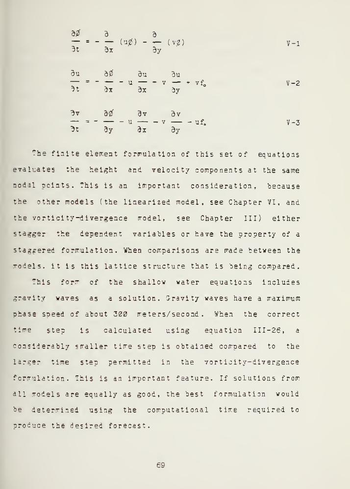
— = (u#) (v0)3t dx dy

V-l

3u d0 du du— = - — -u — -v — « vf3t ox dx c-y

3v d2f dv dv

^t dy dx dy

V-2

V-3

The finite element formulation of this set of equations

evaluates the height and velocity components at the same

nodal points. This is an important consideration, "because

the other models ( the linearized model, see Chapter VI, and

the vorticity-divergence model, see Chapter III) either

stagger the dependent variables or have the property of a

staggered formulation. When comparisons are made between the

models, it is this lattice structure that is being compared.

This form of the shallow water equations includes

gravity waves as a solution. Gravity waves have a maximum

phase soeed of about 300 meters/second. When the correct

tine step is calculated using equation 111-26, a

considerably smaller time step is obtained compared to the

larger time step permitted in the vorticity-divergence

formulation. This is an important feature. If solutions from

all models are equally as good, the best formulation would

be determined using the computational time required to

produce the desired forecast.

69

All Todels use the same domain structure. In fact, the

domain described in Chapter III was patterned after the

iomain implemented by Kelley. Again, this domain simulates a

belt around the earth, with cyclic continuity which

eliminates the east-west boundaries. Rigid boundary vails

exist at the equator and at 30 degrees north latitude. The

domain is composed of a 12x12 point mesh and subdivided into

the right triangular elements illustrated in Figure 9.

Notice that the grid points are not shifted as in the

equilateral element implementation shown in Figure 6.

The following boundary conditions are imposed:

1) - no cross channel flow at the latitude

boundaries .

2) - a geostrophic balance at the channel walls

imposed on the continuity equation V-l.

This model has a simple second order diffusive term in

the equations of motion V-2 and V-3. However, for the

purpose of evaluating these different formulations, this

option was not implemented during the comparison phase.

Initial conditions consist of a single wave in the x

direction and a half wave in the y direction. The initial

fields for the three dependent variables are shown in Figure

12. The maxixum zonal wind perturbation of 5.5 meters/second

is superimposed on a mean zonal flow of 12 meters/second.

70

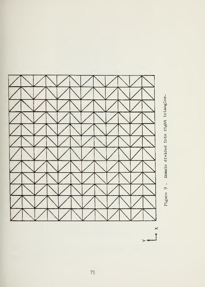
W0)rHtaD

c•H

-t->

•P-Ctjfl

o-pc

(1)

•H-d

G•HCTJ

S

a

ON

0)

•J

71

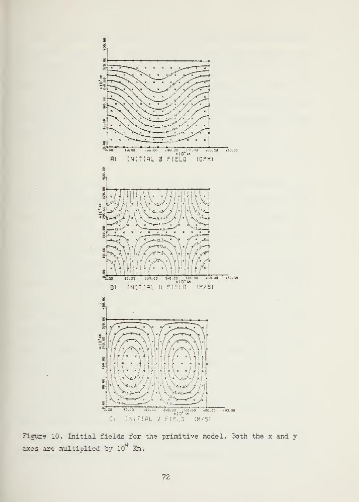
3

Si

^.oo 9j.oo .jo. jo .mu ga >.na

A) INITIAL FIELO (CPM

§

In

u.ca . si:. 30

!3Ii0^iHuvr,/mm*

-*' « yx a x ^*— 8.e < Sc A « -«r-^

§' U.O-' . 3.3"^ ^-tt-O—

J

gt XXXXXXXXXXK*

^ao so.:: .oo.oa 2-to.:a 320. 33 *oo.oo uoo.ao

3) INITIAL U FIELD (M/S)

:i INITIAL V FIELD IM/S)

Figure 10. Initial fields for the primitive model. Both the x and y

axes are multiplied "oy 10 Km.

72

This cursory description of the primitive model mentions

only those significant features that will weigh heavily in

the ccirparisions later. The Galerkin implementation of this

model is similar to that presented in Chapters II and III

and the system of equations is solved using a Gauss-Seidel

iterative procedure. Further details concerning this

primitive model are given in Kelley (1976).

2. RZSU1TS

This experiment involves the shape of the elements. As

mentioned previously, Kelley's implementation subdivides the

domain into right triangular elements, as illustrated in

Figure 9. Considerable small-scale noise was observed by

Kelley in f he 43 hour forecast solution.

The transition from right triangles tc equilateral

triangles changes the size of the domain. With right

triangles, the ax arday grid spacings are equal (300 KM). A

12x12 grid matrix has a length and width of 3600 KM. With

equilateral triangles, the*x and ay grid spacings are no

longer equal. Arbitrarily, the *y grid spacing is held

constant (300 KM) and a new^x grid spacing computed by

u = Ay/ cos (30) V-4

A 12x12 grid matrix with equilateral elements has a width of

3600 KM and a length of 4045 KM.

Figure 11 contains the 48 hour forecasts produced using

both types of elements. The three dependent variables fields

73

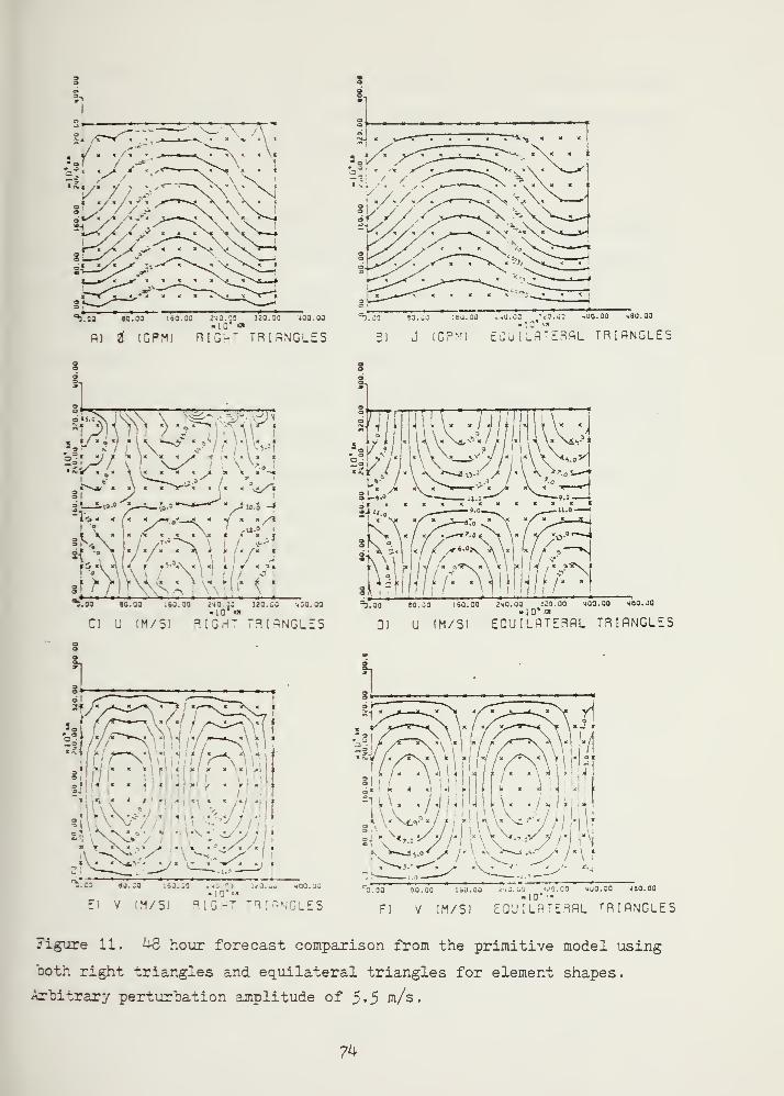
°VC3 JO. 30 '.60.00 2H0.00 320.30 400.00

A) t (GPM) RIGHT TRIANGLES

c3 so. -J ;sj.gj c40.oo 120. aa 4J0.00 4aa.ao10" Ml

31 J [GPM] EQUILATERAL TRIANGLES

!

" y

I - . . j . , « . L . ^ ,

°Voo so. oa .60.00 240.:: !20.;o .00. oo

C) U tM/S) RIGH r TRIANGLES

1

a» oSri

.|Hf7\U fA^1

9 - }H

tvy

X:"~"~— ,—r^

,"T^r-'T"^ .'

.

^.M SJ.;0 163. iO ..*.', .<1..u 400.3010*"

El V IH/Sl RIGHT TRIANGLES

D) U (M/S) EQUILATERAL TRIANGLES

°3 30 SO. 00 160. 00 2'lQ.OO VI. 00 400.30 490.00»10' •"

F) V IM/S) EQU:L^ r ERAL T RIANCLES

Figure 11. US hour forecast comparison from the primitive model using

both right triangles and equilateral triangles for element shapes.

Arbitrary perturbation amplitude of 5*5 m/s.

7^

are compared for each. The small -scale noise that Xelley

observed is present. The three fields shew varying degrees

cf distortions, vhich are especially noticeable along the

"boundaries .

Cider (1981) found that theroot rrean square error (RMSE)

was reduced 22 percent by using equilateral shaped elements.

This improvement is apparent on viewing Figures lib, d and

f. The contours are smooth and the boundaries are

noise free. Eelley showed excellent treatment of wave

propagation by this primitive model. The lowest resolution

grid '6x6) tested by Kelley was within four percent of the

true phase velocity. Changing the element shape had no

apparent effect on the phase velocities.

recause the outcome cf this experiment was a

significantly improved forecast solution, future comparisons

with the primitive model will be made using equilateral

elements .

75

- - 7- V - r T vt S

"": e previous chapter demonst rated how the shape of the

element can significantly improve the solution. Williams and

?ienktewicz (1951} used differently shaped basis functions

c - a linearized e o ua t i o n set to o r od uc e excellent solutions

when applied to the gecstrophic adjustment problem.

Tra'ial staggering of dependent variables in finite

difference formulations has given rucn better solutions to

*'re geostrophic adjustment orocess, and these forms are

widely used in meteorology. Schoenstadt (1930) found similar

result? with finite element formulations with piece wise

linear basis functions. However, staggering nodal points is

net a convenient rethod to implement, especially in

two-dimensions with irregular boundaries* so alternative

schemes are needed .

The implementation of the alternative scheme introduced

by 'illia-s and Zienkiewicz (1931! are presented in this

chapter. As mentioned above, this formulation uses different

basis functions for the height and the velocity fields. One

of r he basis functions is piecewise linear, while the other

is piecewise constant, as is illustrated in ? igu

r

o r e ^TO'ciT^ 1 do ma in •

S 1~

for a

Yfc

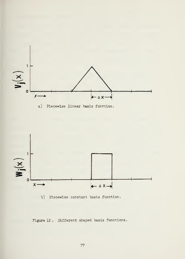
1-

a) Piecewise linear basis function.

-I h

^-A X ->I

b) Piecewise constant basis function

Figure 12 . Different shaped basis functions.

77

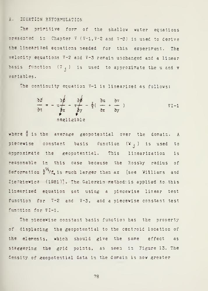
A. ICUATION REFORMULATION

The priritive forrr of the shallow water equations

^resented in Chapter V (V-l.V-2 and V-3) is used to derive

the linearized equations needed for this experiment. The

velocity equations V-2 and V-3 reirain unchanged and a linear

basis function (V . ) is used to approximate the u and v

variables .

The continuity equation 7-1 is linearized as follows:

VI-1

where f is the average geopotential over the domain. A

plecewise constant basis function (V . ) is used tou

approximate the geopotential. This linearization is

reasonable in this case because the Rossby radius of

Reformation jj f\ is much larger than ax [see Williams and

Zie^kievlez (1981)]. The Galerkin method: is applied to this

linearized equation set using a plecewise linear test

function for V-2 and V-3, and a plecewise constant test

function for VI-1.

The oiecewise constant basis function has the property

cf displacing the geopotential to the centroid location of

the elements, which should give the same effect as

staggering the grid points, as seen in Figure 13. The

density of geopotential data in the domain is now greater

7P

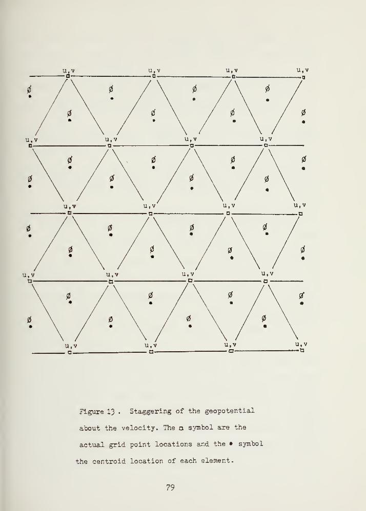
Figure 13 . Staggering of the geopotential

about the velocity. The a symbol are the

actual grid point locations and the • symbol

the centroid location of each element.

79

than the density of the velocity data. Instead of a

gecoctent ial value for each node, there is one averaged

val*.te over each element.

""he final form of the Galerkln equation for VI-1, 7-2

aid 7-3 after performing the tire differencing is:

**l, v - - ..n-1u ; <v 4f 7 i> - u <vj-';i> - •* »$<**, -V *Kay"*x'h>

+ v.u , vV . V. V "> - f vn<V V >1 VI -3

r^/^ n n . „V V >

71-4

This linearized set of equations 71-2, 71-3 and 71-4 is

solved using a ^auss Seidel iterative procedure. It is worth

mentioning that the coefficient matrix <W. ,V.> in equation

7!-2 has all non zero coefficients equal to one, since the

integration of the inner product <W.,Wi> involves piecevise

constant functions.

This equation set is implemented rather than the

equation set 7-1, 7-2 ar.i 7-3 using all of the existing

primitive model cede. The major modification involved the

way that the geopotential was referenced. With an average

geopotential over each element instead of a value at each

node fcr a 12x12 mesh, there are 233 geopotential points

versus the 156 velocity (u,v) points.

E. RESULTS

The results from this linearized model are compared to

those from the primitive model. The initial field for this

experiment, Figure 14 has a maximium perturbation zonal wind

that is one fifth of the value used in Chapter V, Figure 10

.

The mean zonal wind remains 10 meters/second. The 48 hour

forecast solutions for each field are compared in Figure 15.

This alternative formulation shows some promise,

although there are seme minor perturbations in these

contours compared to those in the primitive solution. No

explanation is offered for this small-scale noise, although

possibly the other formulations presented b/ Williams and

Zlenkievlcz (1981) would improve the solutions.

31

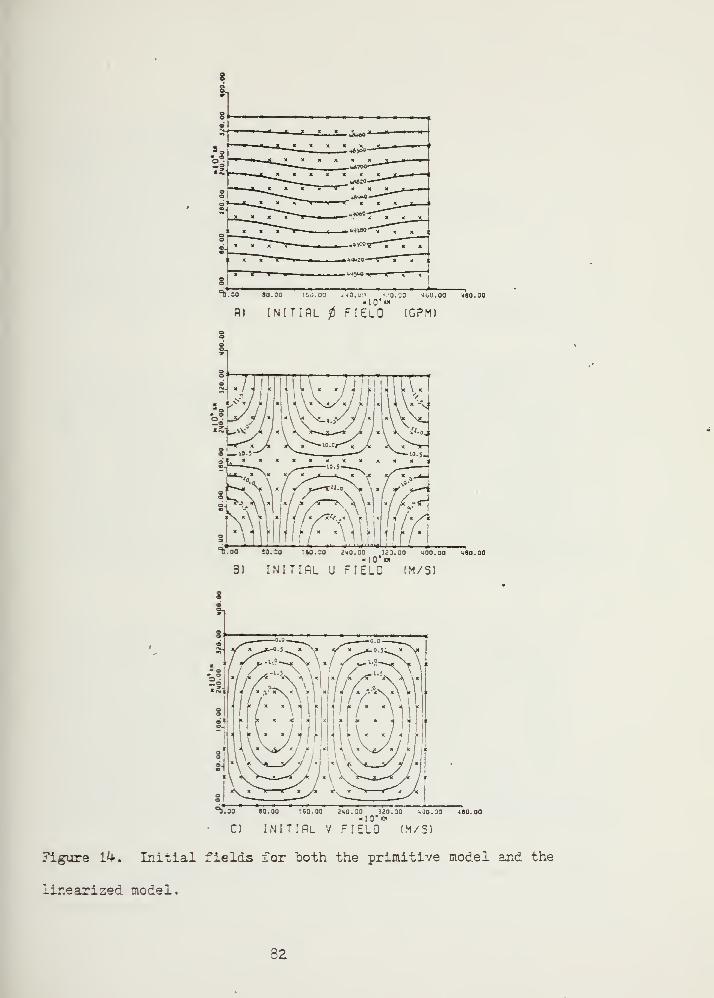
^.00 80.00

R] INITIAL FIELD (GPM)

oo iMO.o" i.m.ca tOU.OO 480.00

\1 !!h; "/v.' .l.'.rir'r/<t • .« I . i i h j. 41 i l ium „ I ..

^.oo so.oo .60.00 iiO.;c ;2:.;o ,00.00 -lao.oo-IO'di

B) INITIAL U FIELD (M/Sl

CJ INITIAL V FIELD (M/S)

Figure 1A. Initial fields for both the primitive model and the

linearized model.

82

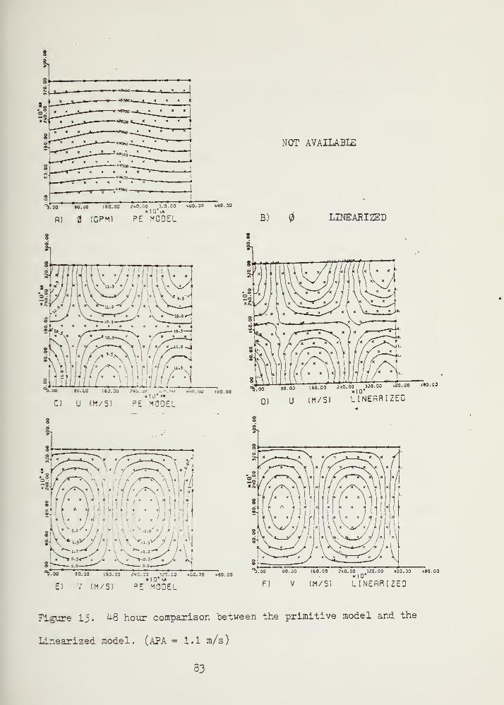
NOT AVAILABLE

'"b 00 SO. 00 160.00 iMO.CO 3J3.BO iOO.OO »ao.oo

fl) t tGPMJ PE MCOEL B) LINEARIZED

aj.JO SU.JO 16J.3U My.

• 10" »CJ U (M/S) PE MCOEL

KiU.UU -190.00

0) U (M/S) LINEARIZED

.1

sir/ \ 11 i

£/'VJuo.su

V (M/S) PE MODEL

b'

.ao ''io. m ' ;so.B3 ;

'

m.:'

3 '

t»;.: 3 ' < 6

'

o.ao Tao.oo"'• 3° 80 -°°

'

60;

00 J"°-°.1Q

.3J0 - 00 <00 - 00 "°- 00

F) V (M/S! LINEARIZED

Figure 15. ^8 hour comparison between the primitive model and the

Linearized model. (APA = 1.1 m/s)

33

tf 1 1 . v:?.TICITY-riVERGZNCI ^CTZL ZXPZRIMZNT

.: s in the previous two chapters, a comparison between

two models will be presented. The results from the

vort ici ty-di vergence model are ccmnared to the results fror1

the primitive model. To fully exploit the differences

between the models performances and indicate the strengths

and weaknesses of each formulation, three domain geometries

i?A three initial conditions are used. All solutions are at

4S hour, except for one case which was extended to 96 hours.

Zrom these two finite element formulations some

additional insight is obtained concerning the execution time

required as the grid resolution changes. Lastly, a "brief

discussion on the sensitivity of the computational technique

is p i en

.

A. TZST DOMAINS ANl INITIAL CONEITIONS

The three domain geometries used in the model evaluation

are illustrated in Figure 16. All domains consist of a 12x12

element -resh with equilateral shaped elements (156 grid

points and cyclic continuity is imposed on the east and

vest boundaries. The domain has dimensions of 4045 KM along

the x axis and 35^3 KM along the y axis.

The regular domain 'Figure 16a) has a uniform

distribution of -rid ooints, with a minimum grid spacing

1$:

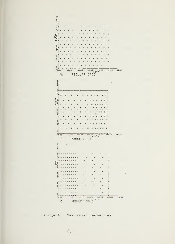
3

X X X X X

X X X X

X X X X X X

X X X X X X

X X X X X X

X X X X X X

X X X X X X

XXXX X X

XXXXXX

X X X X X

X X X X X

X X X X

X X X X X

X X X X

XXXXX*

^.00 90. 30 I SO. CO 2*Q. GO 2^0. CO 400. CO *80. 00

R] REGULAR GRID

* o

2a

X X X X X X X X K X X

X X X X X X X X X

X X XXXXXXX X X X

X X X X

X X X X

X X X X

X X X X

X X X X X

X X

X X X X X X X

X XXXXXXX X X X X X X

X X X X X X

X X xxxxx i

X XXXXXXX X xxxxx

X XXXXXX

^), 00 30 . 00 i 60. JO 2*0. 00 U1 . 00 400. 00 460. 00-13* ra

3) SMOOTh GRID

a 3

b

: x x x x

X X

1 £»« X X X X

X X X X

XXXXXX X X X

X X X X X

XXX

t « « x

XXXXXX X X X

xxxxxX X X X

xxxxxX X X X

xxxxx

xxxxx

X X

X X

X X

X X

X X

X X

X X

X X

3.oo bo. ca .53.;:

C! rsrupt : a

; . t'o.;o .^o.oo *ao.oo«10* «*

Figure 16 . Test domain geometries

.

35

along the x axis of 337 £M . This is the most congenial

loiraia ar.d produces the best results.

The smooth domain [Figure 16b) has a smoothly varying

iistrioution of grid points. This technique allows a smooth

variation of resolution. It was developed by Cider (1981),

who showed how it significantly reduced noise at all

frequencies oo^pared with other variable grid domains.

The degree of resolution variation is accomplished by

selecting an appropriate value for the ratio of maximum

Stretch to minimum shrink: along both axes. The experiments

presented in this chapter use a 2.5 ratio for both

directions. This produces a grid point concentration in the

right -enter of Figure 16b and coarse resolution at the top

srd bottom left of the domain. The minimum grid spacing

along the x axis is 159 Km: in the dense grid point area.

The third domain was the least hospitable geometry for

both models. The abrupt domain (Figure 16c) has a dense grid

point concentration on the left and coarse spacing en the

right of the domain. The minimum grid spacing along the j

axis is 15S KM in the area on the left. The grid spacings

are uniform except for the abrupt change along the center.

Although these three domains are simple in structure,

they are adequate to test both models' performance. To

further enhance some differentiating characteristics between

the two formulations, three initial conditions are used. Two

have previously been described in Chapters V and VI. Their

36

rain iistinguishing feature is the arbitrary perturbation

airolitu<?e AVA) magnitude. The nearly linear case Las an APA

= 1.1 m/s compared tc 5.5 m/s for the more nonlinear case.

All initial conditions have a 12 sn/s mean flew component.

tfith the nearly linear case both models behave well. The

introduction of the rrore nonlinear initial disturbance

illustrated the boundary and computational technique

sensitivity. The third initial condition is the nearly

linear initial field with the wave length equal to half the

domain length. This has the effect of producing two waves

with the domain .

2. ^IST CASI COMPARISONS

The comparisons between models are divided according to

the domain geometry. The primitive model has three fields!

geopotential , a and v. The vorticity - divergence model has

seven fields: geopotential, stream function, velocity

potential, u, v, vorticity and divergence. The geopotential,

u ^tA v will be the only fields used for the comparison.

1 . Regular Case

The regular domain geometry (see Figure 16a) is used

for this first comparison. The initial conditions have an

A?A = 1.1 m/s, as shown in the contour plots in Figure 17.

The 4:9 hour solutions for both models are presented

in Figure 16. As anticipated, all of the solutions have

37

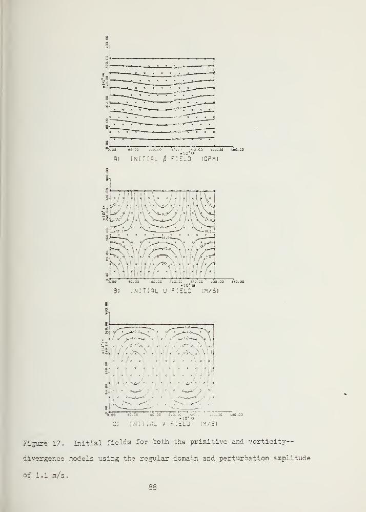
8aSi

NlTIfiL $ FIELD ICPM)

UU.00 490.00

1o

1—V '"

i

,

|\[

«sL^ > /A v\^i^/,/ /A V *m

tl ,11 I ^ I'

ll

^1.00 30.30 150.30 2WO.0G :20.3G <00.30 480.0010*M

B) INITIAL U FIELD (M/SJ

x - — i.i \ >

tfjl - :,^-. yi

< » * . . < , « .

!-

,1* « '^i/ ' ' » . ty

^.OO SO. CO '60.00 210.33 3i3.C ioO.OO -.dCCO• JO'm

Ci INITIAL V FIELD (M/SJ

Figure 17. Initial fields for both the primitive and vorticity

—

divergence models using the regular domain and perturbation amplitude

of 1.1 m/s.

88

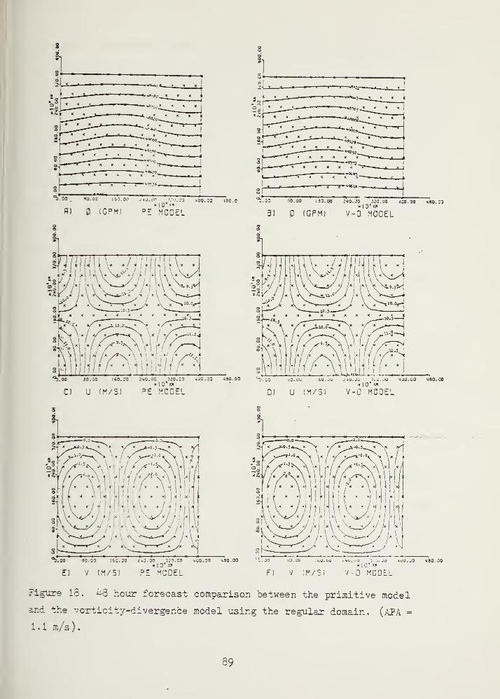
15U-*

^).30 ?a.oa i6o.oi' (40.00 vo.oo noo.oa 430.0-

fl) (GPM) =E MODEL

.03 io.oo 153.00 Jta.oa ::o.oo 400.00 hso.io

B) (GPM) V-0 MCOEL

^.30 50.33 '.53.30 <43.30 JiO.CO ,00.00 430.0010* n

E) V (M/S) ?E MCDEL

Figure 18. ^8 hour forecast comparison between the primitive model

and the vorticity-divergence model using the regular domain. (APA =

1 . 1 m/s )

.

89

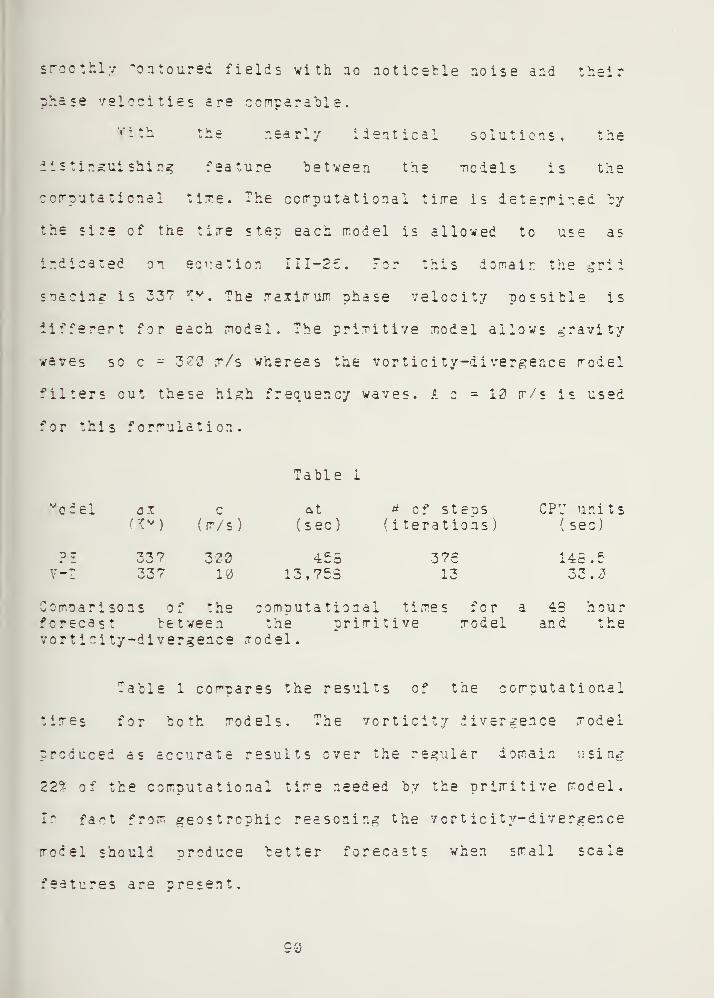
smoothly "ontoured fields with no noticeble noise and their

phase velocities are comparable.

v -th the nearly identical solutions, the

distinguishing feature between the models is the

computational tire. The computational time is determined by

the size of the time step each model is allowed to use as

indicated on equation 111-26. For this domain the gri

i

snacin* is 33? £* . The maximum phase velocity possible is

different for each model. The primitive model allows gravity

waves so c - 300 m/s whereas the vorticity-di vergence model

filters out these high frequency waves. A c = 12 m/s is used

for this formulation.

^odel

D -

?"]

Table 1

<3X c

(m/s)At

(sec)

it 7-z-77

3?010

45513,755

* of steps(iterations)

37c13

CPU units( sec)

145.- p.

Coinoarisons of the computational times for a 4B hourforecast between the primitive model and thevortinity-divergence model.

Table 1 co moares the results of the computational

times for both models. The vorticity divergence model

produced as accurate results over the regular domain using

22*- of the computational time needed by the primitive model.

In fa^t from geostrcphic reasoning the vort icity-divergence

model should produce better forecasts when small scale

features are oresent.

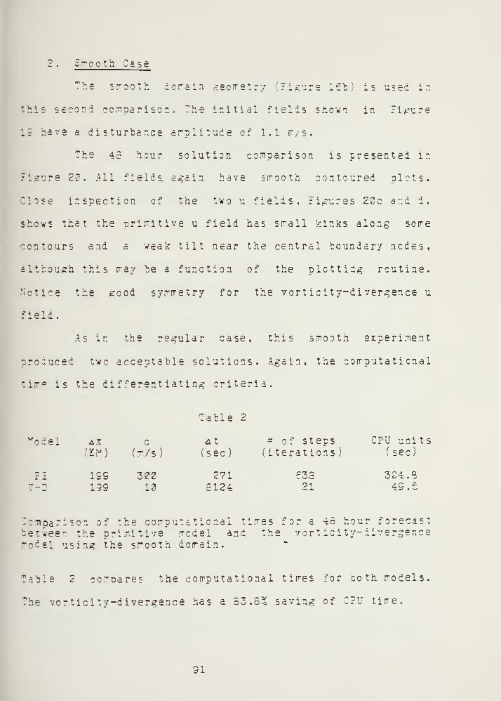
2. Smooth Case

c rp -\ r\ t V omain geometry (Figure 16c s used in

this second comparison. The initial fields shown in Ji^rure

IS have a disturtar.ee amplitude of 1.1 tr/s.

The 48 hour solution comparison is presented in

Ji^'jre 22. All fields again have srrooth contoured plots.

Close inspection of the two u fields, Figures 20c and i.

shows that the urimitive u field has small kinks along sore

contours and a weak tilt near the central boundary ncdes,

although this may he a function of the plotting routine.

Notice the £ood symmetry for the vort ic ity-di vergence u

field.

As in the regular case, this smooth experiment

produced twe acceptable solutions. Again, the computational

time is the differentiating criteria.

Table 2

vodel AX[EM)

c

(T/S)At(sec)

199199

32212

271£124:

n of steps(iterations )

c3821

CPU ujnits( seic)

324 .3

49

Comparison of the computational times for a 43 hour forecast"etwee", the primitive model and the vort icity-divergencemodel using the smooth domain.

Table 2 ccm-oares the computational times for both models.

The vcrtici tv-diver*ence has a 33.8^ saving of CPU time.

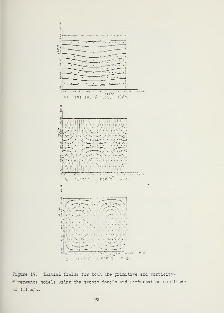
_iJ.

_^

^"

3 —

.

a

-T-_

1- « — «9S39-

^.OO 30. :o

PI) INITIAL t FIELD CGPMJ

.60. 33 JHO.CO 32J.00 400.00 480.00«10*M

i \*\ x * * V'Z IS v

#-'v\1

. . J ... - . 1

^J.JO 30.hu . »••.'.

• 10*'-"

3) INITIAL 'J FIElD (M/S)

• < « «

• - . - « f

-] u . ,

i>

^a.oa lo.ca iso.co

C: I'.:-:-- r :E_: (M/:

Figure 19. Initial fields for both the primitive and vorticity-

ilvergence models using the smooth domain and perturbation amplitude

of 1.1 m/s.

92

•

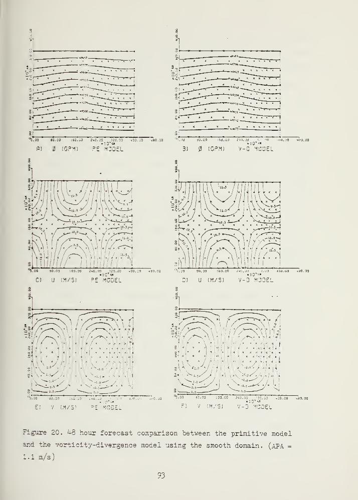
oo jo. 30 16O. JO Jho.j: >20.00"10*"

RJ Z !GPM) de mgoel

jo. jo «ao.30 u do.oo :gu.uu riu.uo i.'u.un K'U.uo xmo.oo«|0" ««

3) (GPM) V-0 >1U0EL

?j.oo so. co ;so.:o no. oa ija.aa .oo.:oIC'w

C) U [M/SJ oc- MODEL

Tj.00 80.00 !60.00

0) U (M/S) V-0 MCCEL

J. 00 100.00 400.00

.-

< «

i [ \'

I' *. • ' *

'

H. M

E) v iM/si pe v\::e.

ifU". N J,

;'•'-•' '

. .v.'..-.','

! \" /Will I

.03 dC.33 160.00

Fl V [M/SJ V-0 M CGE

•33 120.00 .33.30 -aO.OO«I0 «

Figure 20. ^8 hour forecast comparison between the primitive model

and the vorticity-divergence model using the smooth domain. (APA =

1.1 m/s)

93

In an effort to contrast the computational accuracy

at the rodels, this experiment is repeated using the rore

nonlinear initial case. Figure 21 shews the initial fields

with a?A = 5.5 rr/s . This larger initial disturbance is

reelected in the greater geopotential amplitude and

magnitudes of the contour lines.

Figure 22 shows the 45 hour solution comparison. As

in the rore linear case presented above, all of the plots

have smooth contours with no noticeable noise. The

vorticity-di vergence geopotential field, Figure 22b, has the

rid^e extending farther north, and flattening of the

southernmost contour, than does the primitive geopotential

field, Figure 22a. The mean geopotential heights for both

models have also increased. The primitive mean geopotential

is now 49£8<? gum and the vortici tv-divergence geopotential

is 49630 gpm.

These two discrepancies indicate that the boundaries

are not handled accurately. Turing the implementation of the

vortici ty-di vergence model, treatment of the boundaries was

the most troublesome phase. The vortici ty-divergence

formulation is a complex equation set and time limitations

restricted further investigation of mere sophisticated

boundary conditions.

This same initial condition is now extended to a 96

hour forecast, which is shown in Figure 23. The mean

vcrticity-divergence 2-eopotentiai increased to 49S00 gprr

,

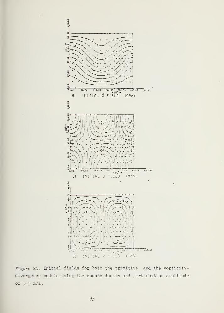
*1

^>.oo so. co 160.30 2*o.:: no. ao tao.oo 7ao.:o

fi] INITIAL FIELd" IGPM)

-! sa >/

« « # '« \*3.o i^« > x \* * a.o_i

:i x n n x x k « x x » < x

>-H'>.v. • /*— "-—»—« « *>^**-1

a i ...... a. . t . —t—. *-

^.jo 30.oo iso.oo <4a.;3 j;o.go -.co.oo »oo.oo• 10*"

B) INITIAL U FIELD IM/SJ

•.-..-.'j a « « < I la... Jlj[\\\\

i*. x\ *--»"xy » ,

|fx / x x * art

ft I::•'""<

> a K all a

« i < « » < - k

/. . .

":. BO 80. -0 ;. j 00

'10' UK

.00 .80.00

o initirl v r:

::_: im/sj

Figure 21 . Initial fields for both the primitive and the vorticity-

divergence models using the smooth domain and perturbation amplitude

of 5.5 m/s.

95

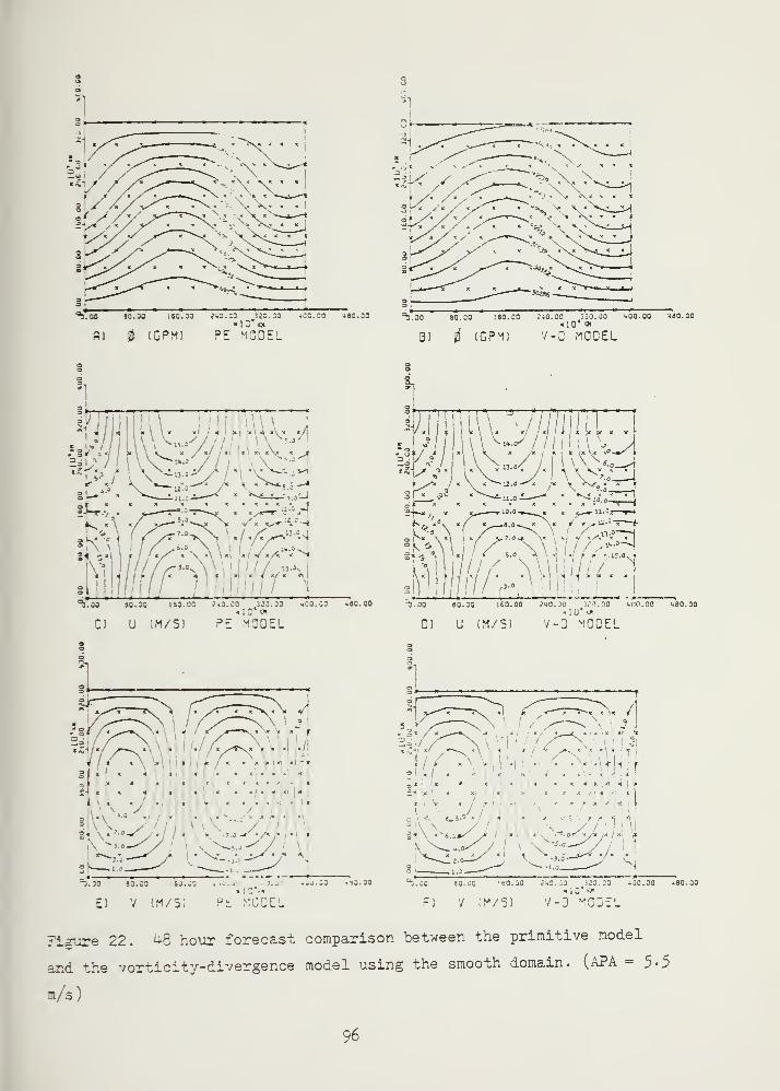
^.m aa.oo ;sa.30 243.33 323.30 «cc.30 480. oo

lO'nfi) (GPMJ PE MODEL

^J.00 SO. 30

O U (M/S)

iso. os ;*o.oo 323.00 -.co.so

lO'nPE MODEL

1•

. ww.w;'

T.30 93. 03 .SJ..

E) V (M/Sl 3 - MODEL

^.00 30 30 160.00 240.00 320.00 400.00 480.00*10* a

3) $ IGPM) V-D MODEL

HZK f^rU.Oj I-t

"3.00 S0.3C

0) U IM/S)

JlL-1'.£0.00 240.00 370.00 4110.00 uSO.OO

c 10* KM

V-D MODEL

: / .

' .

' :. /vMVNUf

m •

-1

I

l

i7

80.00 '50.30

V [M/S)

!40. 30 320. 3010" K»

V-D MODEL

400.30 -.80. 30

Figure 22. <*8 hour forecast comparison between the primitive model

and the vorticity-divergence model using the smooth domain. (APA = 5>5

m/s)

96

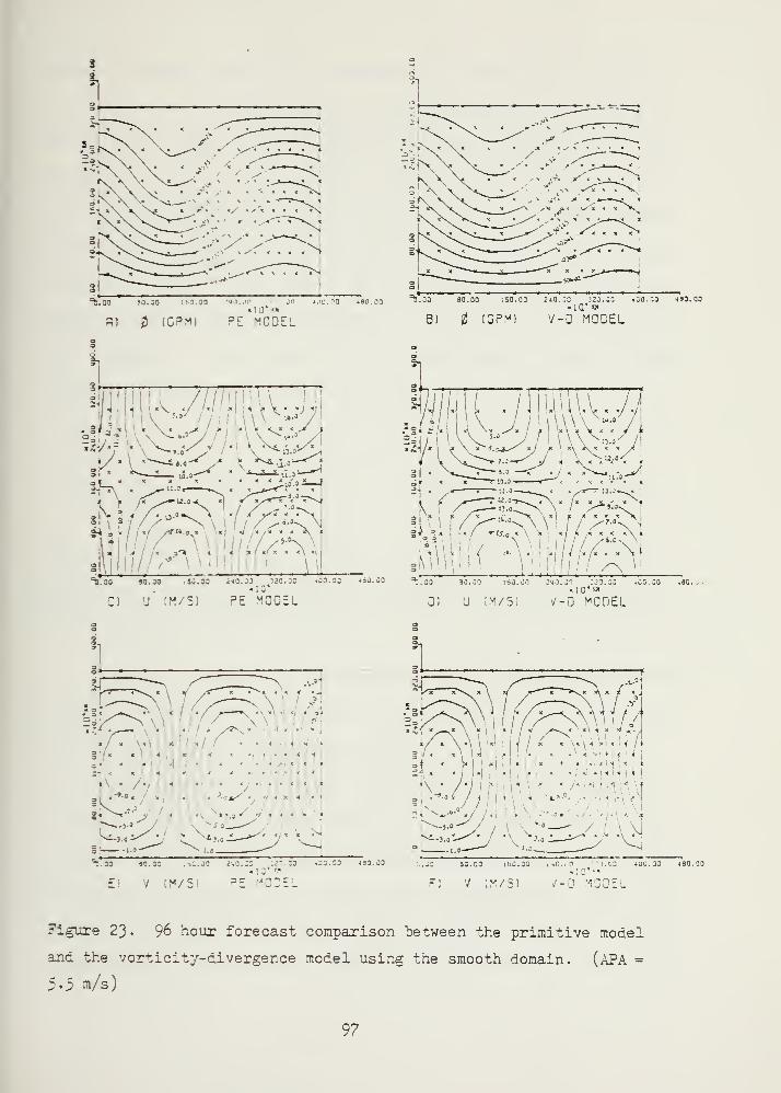
J

^.00 50.30

3) # (CP^l 3E MCOEL

.an jno.no 480. oo10' <«

^j.oa ao.oo :so.oc 24.0.00 320.00 -.00.00 490.00«1Q' **

B) (3PM) V-0 MODEL

o u :m/si =e model

^).C3 30.00

D) U iM/S) V-0 mqoEL

SO. CO JHO.ai J20.00 -CO. 00 <dO..lO'w

. 01

J .

.' .-J

..... .

§ « « - - 4 < -

i' ' " ' ' f--. « « * < 4 . . < 4

\\\ •

'•. '"

k,; si

.30 so. as 160.1

E) V (M/S)

,j.:a ^30.00

3E MODEL

, \.....

.. , *.«. ./..U\,

bO.OO <r4C. .:n VII. CO 4UU.00 480.00a.oa ao.oo

F) V (M/Sl v'-l'-y!ODEL

Figure 23 • 96 hour forecast comparison "between the primitive model

and the vorticity-divergence model using the smooth domain. (APA =

5-5 m/s)

9?

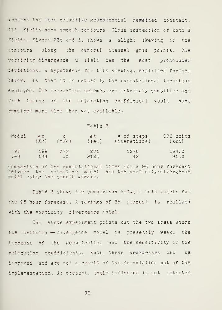
whereas the mean primitive geooo tential regained constant.

All fields have smooth contours. Close inspection of both u

? * e .. z A — -4 . W '2c and *i, shows a slight skewing of the

contours along the central channel grid points. The

vorticity divergence u field has the rost pronounced

deviations. A hypothesis for this skewing, explained further

below, is that it is caused by the computational technique

employed. The relaxation scherres are extremely sensitive and

fine tuning of the relaxation coefficient would nave

rehired more time than was available.

'able 3

Vodel A x r

(m/s)4 t

(sec)

199199

2Z212

2718124

# of steps( iterations )

127642

CPU units(sec)

594.291.0

Comparison of the computational times for a 9€ hour forecastbetween the primitive model and the vortici ty-divergenceT ccel using the smooth domain.

Table 3 shows the comparison between troth models' for

the 96 hour forecast. A savings of 35 percent is realized

with the vorticity divergence model.

The above experiment points out the two areas where

the vorticity — divergence model is presently weak, the

Increase of the geopotential and the sensitivity :f the

relaxation coefficients. 3oth these weaknesses can be

improved and are not a result of the formulation but of the

implementation . At present, their influence is not detected

93

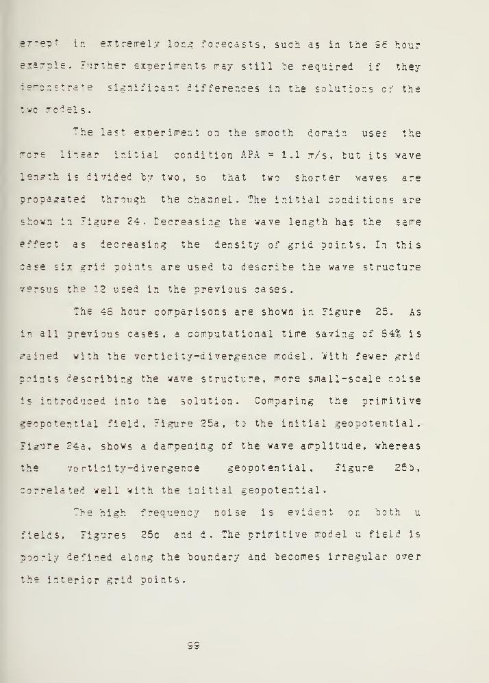
ex-ep' In extremely long forecasts, such as in the 96 hour

exaxpie. Further experiments ray still be required if they

demonstrate significant differences in the solutions cf the

two models.

The last experiment on the smooth domain uses the

mere linear initial condition AFA =1.1 m/s, tut its wave

length is divided by two, so that two shorter waves are

propagated through the channel. The initial conditions are

shown in Figure 24. Decreasing the wave length has the same

effect as decreasing the density of grid points. In this

case six grid points are used to describe the wave structure

versus the 12 used in the previous cases.

The 46 hour comparisons are shown in Figure 25. As

in all previous cases, a computational time saving of S4% is

rained with the vcrticity-divergence model. With fewer grid

points describing the wave structure, more small-scale noise

is introduced into the solution. Comparing the primitive

geopotential field. Figure 25a, tc the initial geopotential ,

Figure 24a, shows a dampening cf the wave amplitude, whereas

the vo rtici ty-divergence geopotential. Figure 25b,

correlated well with the initial geopotential.

The high frequency noise is evident on both u

fields, Figures 25c and d. The primitive model u field is

poorly defined along the boundary and becomes irregular over

the interior grid points.

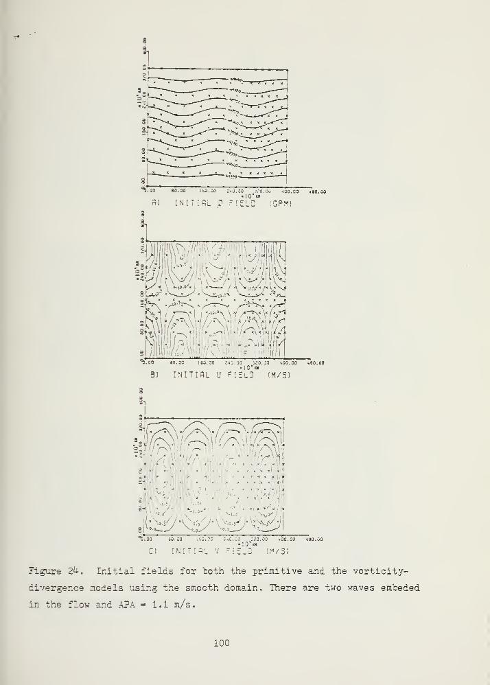
Si

IO'kii00.00 430.00

fi) INITIRL p F [£L3 ;pmi

.Jib.'. ] :- :%2f

/j//L\\ // J\\ s? '•

i

/lfl\*xi«•J/ k\\x/ «. < C- < « .< jl> M-oi

- .>*

it • r iwlj " it— Maui~.oo ao.oo tsa.oo 2<<o.oo ..;..; 400.00 4SO.00

B) INITIAL U FIElO (M/S)

i- . . . - . . . . 1 . . ,

- „..«... - .

I

-J i • £ \

;

=b. 30 SO. 00 1 60. CD

C) INITIAL V [ELC (M/S)

0.30 :<C30 400.00 490.00

Figure 2fr. Initial fields for both the primitive and the vorticity-

divergence models using the smooth domain. There are two waves embeded

in the flow and A?A = 1.1 m/s.

100

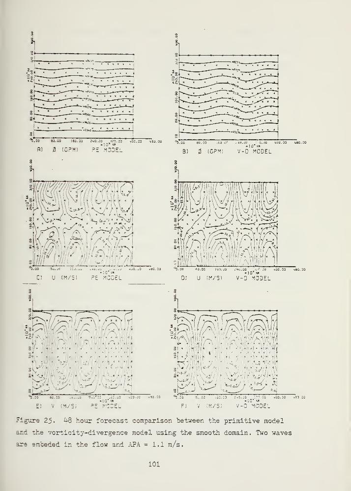
*1

_ P il « KB

T.JO 30. JO ISO. 30 2>.0. JO 323.30 -.00. 30-10* «

P) IGPM] PE MODEL

- »i

ii I.i

ii i« i

t.oo au.oo if.fl.oo .jo. lw i 'o.iio nnu.oo aao.oo10" a

8) ZJ (GPM) V-D MODEL

3

*]

——,-_—._,? - 1

(J i \ fcl r -

r ?* * / x \ x / J \ V x 'xl * V_i

S** yi x1—-T^_. « -.-—^* J v/r^T

IS / .,-0 .^^7^1 f, TV x/./TX:

ji t ii i .i . . . , /// i— .

—

j_i i_ui , 1,! ii —imU i i., ii .n i,

i i Uuil'VoO M.JU IfiU tHU.UU ....ju .0O..1O

C) U (M/Sl PE MODEL

80.30 ^.30 dfl.00 Itill.jU .10.00 1^0 OU 400.30 480.3010' n«

D) U (M/Sl V-D MODEL

*1

"^x^\ < / / *_^ xi -x « i k A x i \ *A

i

if* I r . > . . .

:

ui . .

' «

- . . . , 4 ,.,...,M y-w •.:'".::.S. .......

I 4: ' »i X1 M « •

• —A *9\U k j - j ->-

LJ^« 1 . 1 . < .\^ . '

' / ' ^ , ,

i "..0,

„ I 4 ^.r ., -'. t| . . ,,y .„J i' ;;

Vx

*.(*-

iL-w,J%.0I H.OC [60.;

EI V (M/Sl10' oi

PE MODEL

.30.30 .-iO.30 30 -!..:: iSO.OO Jv.O.00 3J0.00 .00.30 .80.3010* w

F) V (M/SJ V-0 MODEL

Figure 25. ^ hour forecast comparison "between the primitive model

and the vorticity-divergence model using the smooth domain. Two waves

are em ceded in the flow and A?A = 1.1 m/s

.

101

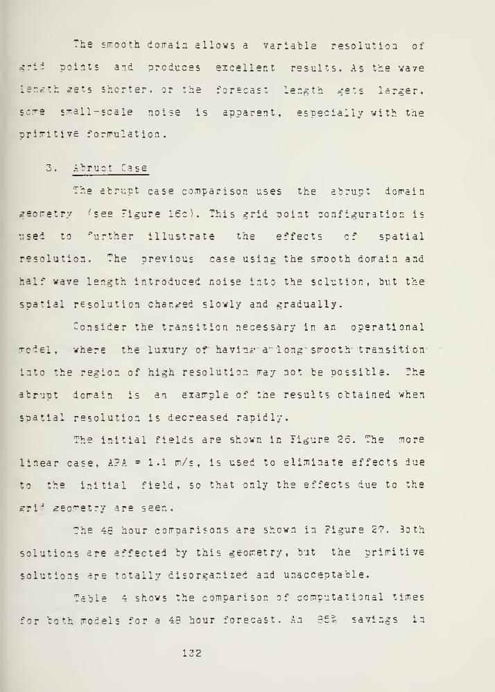
The smooth domain allows a variable resolution of

grid points and produces excellent results. As the wave

iensth sets shorter, or the forecast length gets larger,

sere s^all-scale noise is apparent, especially with the

orimitive f ormulat ion .

3. Arruot Case

The abrupt case comparison uses the abrupt dorrain

geometry 'see Figure 16c). This grid ooint configuration is

v.sed to -"urther illustrate the effects of spatial

resolution. The previous case using the smooth domain and

half wave length introduced noise into the solution, but the

spatial resolution changed slowly and gradually.

Consider the transition necessary in an operational

model, where the luxury of havi-n^- a- long smooth- transition

into the region of high resolution may not be possible. The

abrupt domain is an example of the results obtained when

spatial resolution is decreased rapidly.

The initial fields are shown in Figure 26. The more

linear case, A?A = 1.1 m/s , is used to eliminate effects due

to the initial field, so that only the effects due to the

£ri J ^ec^etry are seen.

The 46 hour comparisons are shown in Figure 27. 3oth

solutions are affected by this geometry, but the primitive

solutions are totally disorganized and unacceptable.

Table 4 shows the comparison of computational times

for both models for a 48 hour forecast. An 3££ savings in

122

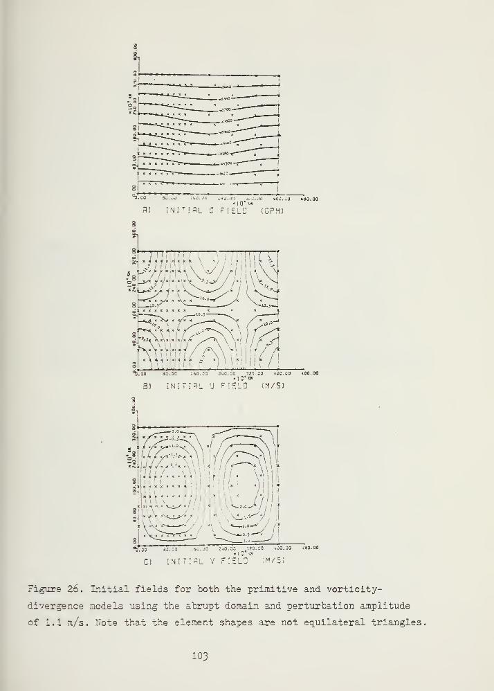
p) ;Ni T ;ai c field (gpmi

B) INITIAL U FIELD JM/S

/ >~^ \ r

1W-WiHrrr"""]Ur......

* + » "^-C.i.J'"* <5^ \^7^.30 ic ja 240.30 920. ca ,00. ao -lao.ao

ilO'w

C) INITIAL V FIELD IM/S)

Figure 26. Initial fields for both the primitive and vorticity-

divergence models using the abrupt domain and perturbation amplitude

of 1.1 m/s. Note that the element shapes are not equilateral triangles

103

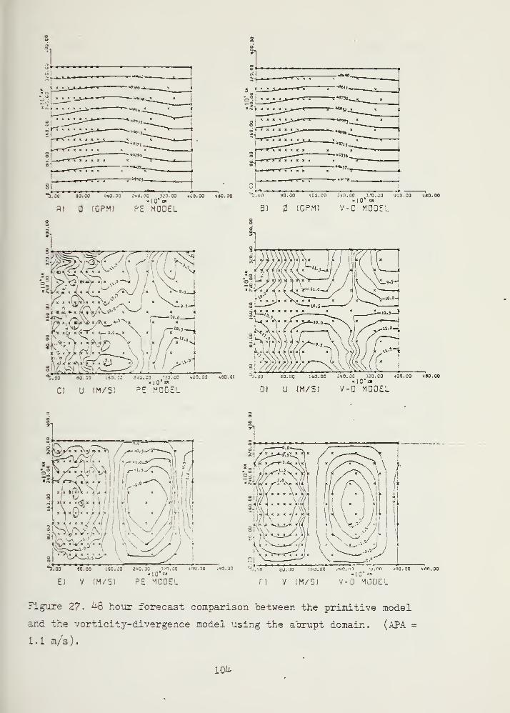
JO 80. CO 160.30 cVO.JO 3.M.0O10'

w

R) IGPMJ PE MODEL

CO. 00 48.0.00 ~J.uO 90.00

B) iCPM) V-D MOOEL

100.00 ."'40.00 VO.UO 4UO.0O *ao. 0010' KK

-k^^r^r /f r*'ft N*

3

S9^ ; '

A w />"> A o' \ J

U.J

t.jo ao.:o*.—I— * —

.. ;: ,; o.co 400.00 <ao.oc tj.ou so. go :so.oo jho.oo jjo.oo too.oo <eo.ooi n" n »lC'a10'

«

"1C a

C) U (M/S: PE MODEL 0) U (M/S) V-D MODEL

V0" ' ' '

six J < i a

b Hy> «, »\

«—>, « i « • -

.

. < .»

°a.w so. oo i60. :o j^o.jo :>t.do <oo.:o .?o.oc«10'«

E) V (M/S) PE MODEL

f in ao.jo ji.ij.no i»MO.nn

F) V (M/5J

n vino. 00 gflo.oo

10 «»

V-D MODE!

Figure 27. ^Q hour forecast comparison between the primitive model

and the vorticity-divergence model using the abrupt domain. (APA =

1.1 m/s).

10^

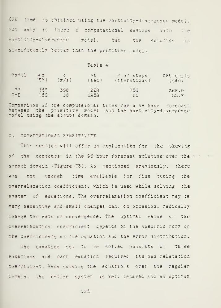
CPU tire is obtained using the vortici ty-divergence model.

only is there a computational savings with the

vortici ty-divergence model, but the solution is

significantly better than the nrimitive model.

Table 4

A X'7v)

c

(m/s)At

(sec)

16?168

3201?

2286558

v o^el ax c At # of steps CPU unitsat ions) (sec)

756 368.925 55.7

Comparison of the computaional times for a 48 hour forecastbetween the primitive model and the vcrticity-di vergenceroc" el using the abrupt domain.

C. COMPUTATIONAL SENSITIVITY

This section will offer an explanation for the skewing

of the contours in the 96 h~our forecast solution- over the

smooth domain 7i<?ure 23). As mentioned previously, there

was not enough time available for fine tuning the

c verrelaxation coefficient, which is used while solving the

system of equations. The overrelaxation coefficient may be

very sensitive and small changes can, on occasion, radically

change the rate of convergence. The optimal value of the

overrelaxation coefficient depends on the specific form of

the coefficient of the equation and the error distribution.

The eouation set to be solved consists of three

equations and each equation required its own relaxation

coefficient. When solving the equations over the regular

domain, the entire system is well behaved and an optimum

125

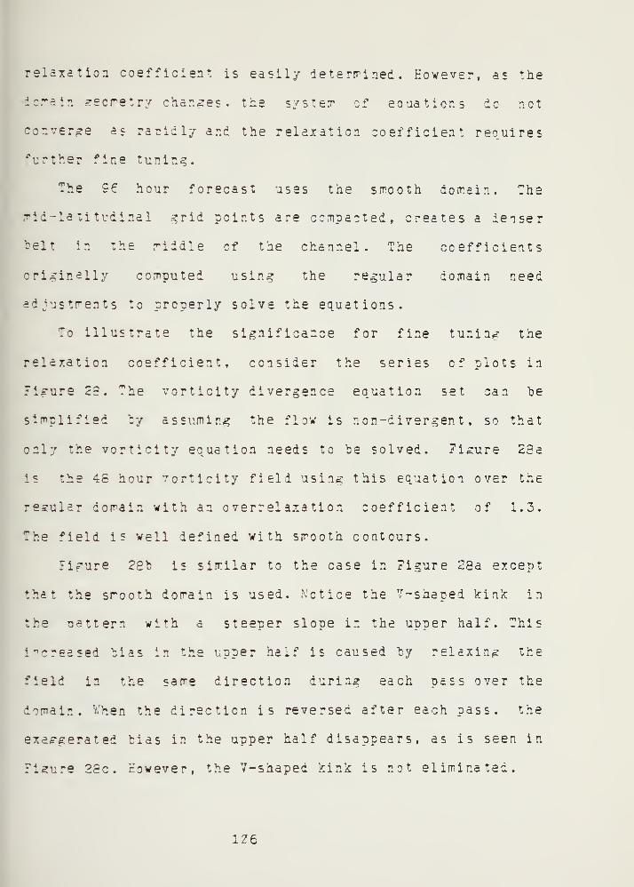
relaxation coefficient is easily determined. However, as the

ioirain geometry changes, the system cf equations do net

converse as rapidly and the relaxation coefficient requires

further fine tuning.

The 96 hour forecast uses the smooth domain. The

f*i d -la ti tudinal grid points are compacted, creates a denser

belt in the riddle cf the channel. The coefficients

originally computed using the regular domain need

adjustments to properly solve the equations.

To illustrate the significance for fine tuning the

relaxation coefficient, consider the series cf plots in

Figure 28. The vorticity divergence equation set can "be

simplified by assuming the flow is non-divergent, so that

only the vorticity equation needs tc be solved. Figure 23a

is the 46 hour vorticity field using this equation over the

regular domain with an o verrelaxa tion coefficient of 1.3.

The field is well defined with smooth contours.

Figure 28b is similar to the case in Figure 28a except

that the smooth domain is used. Notice the V-shaped k:i nic in

the pattern wi*h a steeper slope in the upper half. This

in creased bias in the upper half is caused by relaxing the

field in the same direction during each pass over the

domain. When the direction is reversed after each pass, the

exaggerated bias in the upper half disappears, as is seen in

Figure 2£c. However, the V-shaped kink is net eliminated.

1Z6

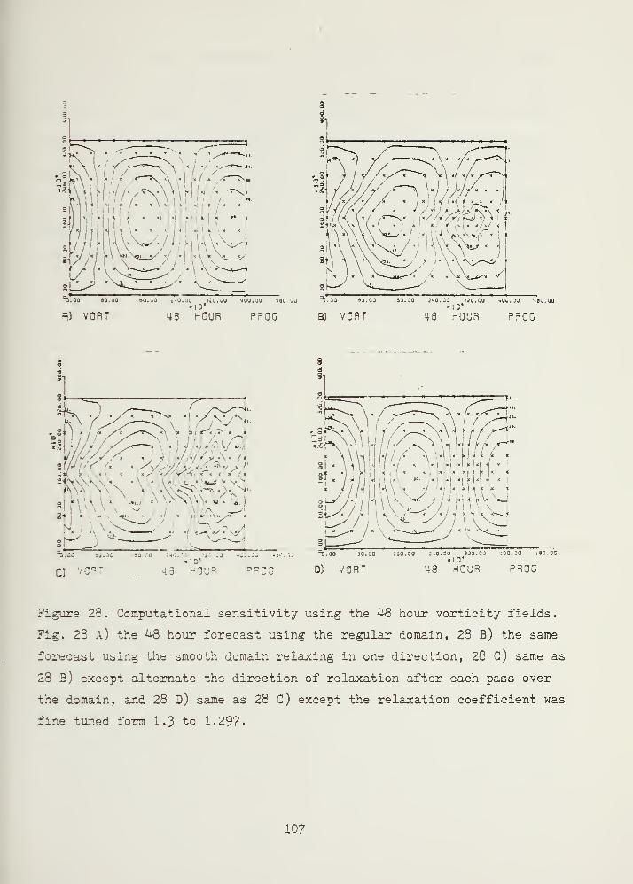
3

1

*1

.lyi//.

^i.ao ao.30 i»o.co nQ.:3 ko.oo 400. :o 480.co

R) VORT 48 HOUR PROG

^b.oo 'o.oo 60.20 240.33 ?20.co ,00. oo 490.00

B) VORT u.8 HOUR PROG

W/T?\) ::::::.

! • '

-- -"-

T.30 iO.JO :S0.30 240.30 323.33 ,30.30 <30.3G-10*

•' = 0) VORT 48 HOUR PROG

Figure 28. Computational sensitivity using the 48 hour vorticity fields.

Fig. 28 A) the 48 hour forecast using the regular domain, 28 B) the same

forecast using the smooth domain relaxing in one direction, 28 C) same as

28 B) except alternate the direction of relaxation after each pass over

the domain, and 28 D) same as 28 C) except the relaxation coefficient was

fine tuned form 1.3 to 1.297.

10?

Varying the relaxation coefficient from 1.3 to 1.297

produces the much improved solution in Figure 28d . If the

relaxation coefficients for the other two equations could

alsa he fine tuned, it appears that improved solutions would

result. There are also other relaxation techniques available

that have potential for improving the solution while also

sonrerging at a faster rate. Some of these techniques will

he tested in the futuer usin^: this model.

128

VIII. CONCLUSIONS

T'his research investigated different finite element

formulations for the shallow water equations. The

two—dimensional dorrain was a channel which simulated a belt

around the earth. Analytic initial conditions were used to

simplify the comparisons. Two formulations were examined;

one using different shaped "basis functions and the other

using a different form of the equation. Zach was compared to

the primitive fornr of the shallow water equations that was

developed by Kelley (1376).

The use cf equilateral shaped elements which was

su^ested by ~r. .

V .J.F. Cullen significantly improved the

solutions compared to lelley's model, which originally used

ri?ht triangles as basis functions, *ost of the other

studies in this thesis used the equilateral triangles.

Williams and Zienkiewicz (1981) suggested the use of

piecewise linear basis functions for the velocity field and

piecewise constant functions for the height field. This

formulation was tested with a linearized continuity

equation. The results were poorer than those obtained with

lelley's model .

v ost of the effort in this thesis was devoted to

ir-plement at ing and testing a vcrticity-divergence model

1 7Cx C H

sirrilar to the ones developed by Staniforth and Mitchell

fig 7 ?} and Cullen and Hall (1979). Several tests were

presented which compare this formulation with Kelley's

rod el. It was found that this model executes approximately

one order of magnitude faster than does the primitive

formulation ^sed by Kelley. Secondly, as the spatial

resolution between grid points decreases, this formulation

oroduces a solution that is far superior to the primitive

form. A disadvantage is its computational sensitivity, which

requires fine tuning in solving the elliptic equations for

certain geometries. It also requires 25 percent more

computer storage, due to the more complex equation set and

the additional variables that are treated.

Implementation of finite element models is not easy.

Fowever, there is a lot of generality and redundancy

imbedded In the computations. Versatile modules were written

which significantly reduced the effort in implementing the

vortici ty-d

i

vergence model.

further research is suggested using this finite element

formulation. It has accurate phase propagation , is able to

handle variable grid geometry, reduce the small-scale noise

and decrease the model's execution time. Specifically more

ad.va.r.cei methods of solving the elliptic equations should be

investigated. Finally, the formulation should be tested with

small-scale forcing, where its advantages should be most

evident .

112

.

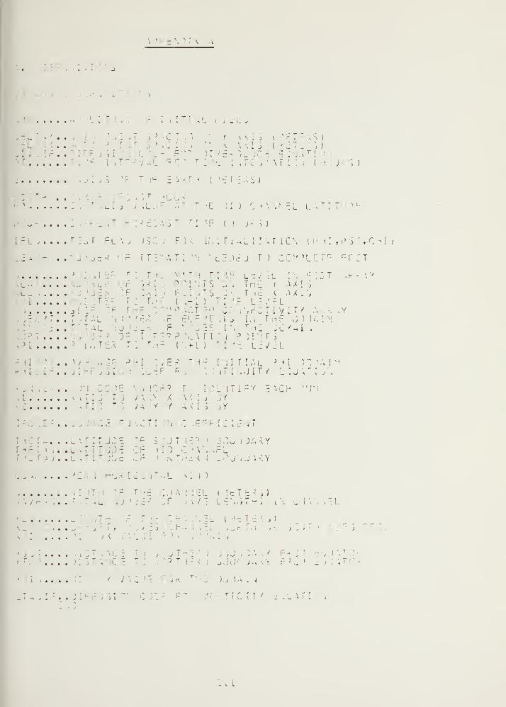
. . . I .

I - .

L • • i

.

r-iF i m

* j ^

' i

i- -

L. .

.>

1 -

< \ X I i ( > t

I

F ; . t '. _ - ~ ~

r. . . .

-

, \ [;..{• j >

i

ii.jj T - ~ 1 •(

-.'.,)

: .

r

ili j /ml >E !l.) C iA.\l\El LAT! T >F

: _ .

* -.-:;.; ~ ~:

r-

i i j k s j

r :.,r FLAo ISEO r irJiTiALU u icn u n , p s t f C --i I i

.^- ••• f it: ATI

'

. L"

It J t ] cc ip L E FCST

j

: . ;

_~ r. r • th thsj le^/el : .

i: :: t .

5^ ^i*|TS G.'j The r AXI 5:f ; x : : f ; . its j r i- c jxisr: t.- : i\-i j t :

-- levelj::

-:f r -- compacted j. inectivity a.-.say

; iTAL i

> j

;

'

. i ^ [.i ruF 13 HA INf • =s i ,

r.-1 ; j c y a I j

: 9. Pr L A r I C J P • 3 IN T ire Tn z

( "ii- 1 ) : :• -. lev el

r~TAL NU

3

»IO .--- - -

r I-J T J ; \ A < \X I

";

tg;a:<yya<ISl>y: - f j \ c t i - : efficient

INITIAL MI ) C -1 Ai T I \ ij I t y '_

; j ; r ;j

'

JY

F 5 \JT )-:'' 3ild I )A*Y

L ; T IT jjij c . F • -

: -.,_• j ..;:-: Y

. r I T JD ELATITUDE

. r-Uk [Z J iT.-,L l 1

'

f" - rne : j . ; . i :r[ : ;;]

r A L _ - F r W E L E

'

"* y> T n 3 i L IW ) E L

th - r - -•]- i•'- 1_ •

* i

j- . . . i

• - . . J . /"

' J

iGT a ; jT -

. jjv)a;;y Fk;; i ;-j jatgI [ 3T; CE " W T i- < ! jJUf Jm -.'r :" -

. '

-.

. . - iirr : :: f r

; C I T /£ ; L A T I

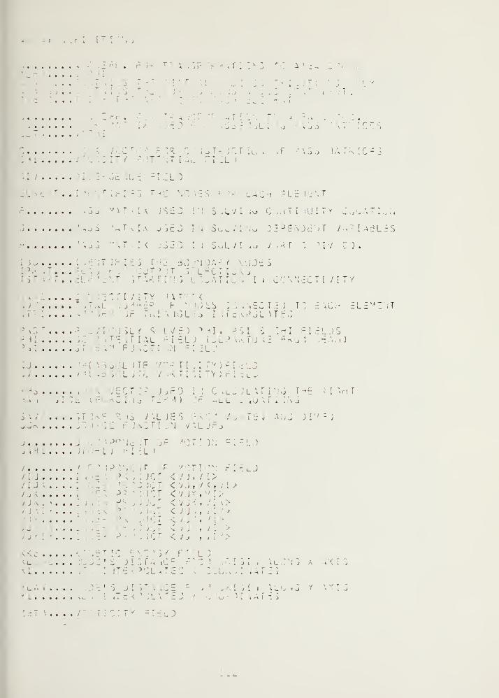
-[T

I

- n1 >:

t i

- -

J •

j <

/ 1 j ;

i j

• \ . ;r «t :

i

• ".

J

-\ : [

-t i :

I . i J T I-

.j \JCT Ic'i i F \ j i I A T r» [ C F 5.

"

. ; it > T" -.r [ .... fi :lj

:e r: 'l :

:•

r;.- :

::

~ •: '.: : ; - each ele il\t

.33 '•'•: \ JSEC E'l SJLVi io C..,i: UIT> lQUATI-jIj

'i3S 'ATX IX jjc. I I SCLVI ivj 3EPE-NJE IT /AF. IABLES

« _) o "«"»< Jjl'Ij IN 5 ^> L / 1 io j i ri T "» ) I V L ) .

T : : -. 3 r • • -~

.

-.-. - < jje s

JT:>:JT 3.ELFC7 IG\3'

•

' ITAK7ING .TiCATICr. I j CCXNECT I 7 I TY

; : c t i 7 i t v '• \ t f ' <

".".:. .,•..- f jes :...e:i.:j t: each e l £'-1 i i t

F Fhl-VJGL I IfcKPUL \7£C

I SLY S IV E J 'HI ,3 SI •: :hi r

1- !

.

1"

r.

• [ A l :

I E L : ( D C ;

J

. ,'

cj <:~: .:: '-: eld

('

• S ' L , T - R T I C I T Y ) F I :f L D

\-t\ h: A ,*I J

.. ; _ . < s 7IEI7Y) rlcL

. . ,: •- J3F0 I : c ;lc Jlat riG r ie I

: I ;'--') IF ALL - ,/A, ;M3

?. HS /AL JES • /CxTE j AN J j i

:)

S-r. J r\ •: E F . J \C T I I / A L J E 3

J . : •Jn 'i_ .T }F * IT! ; . F I f=l_l3

H - L I FI :LJ

;h r

' p- "i*

i E i r f---:•

f I e l J5

v j ; j c - < v j # / 1 >: .: »h :j jot < vj, •</•<, yi>

-> ;'

: ICT <VJ*,VI. < V J < t / I .<>

... <7J \, 71 >

: jc t <. v j , / ! >

r> ,.:"<; j » /

.

' N

•.

; t : : E E '.G V F I EL ]

:' i JlS7A.iCF -" Z ' ";IGIN \l1 ITE 5GLATE r

J ; XL.i )I IA7E3

: • S J I > 7 A.* 1 C E.^ . ; ,7: ' .'_ \ "E

r ! C [TV = I E L J

. - _

] Jj - I .

1-- I j

I # • * • •

.-

;

. j i

-

J1 1 : i

IS

: r .

/)• -

. » .

.

L * 1• >

-~

,

j'-; . - * I

-i ; : L > < L h

z\ • . iiL • j .»...: :

:

,

r ir s l?t «: I- - " "

: :- i.

j... :.E .

• r : _ ;_ u v i r i

\i

[

t \ fi vti •-

.

.. . rv • r i

; .-•: r s . , . ,

> • t L O

ITZZ"

'. r .'

. ; .\ n l FjC I^l _ J J -«

'

I."

' . . ..._ + '

i "J J» 5 / '- U \ i_L: S =ijh 1.. . i.il. WVLYJIS L6J; •

. : .a t i i r i l -. i i i y s i s :

r

: ,: : lat.es > j i .~>

:j.< ia^ij.uc \ ialysi s , j :

:'

"i vl i : . ; >hi, r> s i uj ;;-»! - i -:l ; ,.

.

i t : \u i : -; i )el 5

. - » if r:

;

. [ ri XLIZ^S U.L 3LJQAL /A-*I \.iLtS1

-

"S *LL

r Ti :>c ;-JC F3

: > jtes rHs i it-: .

i

:i *t :- ;ki j ^chts

• •«••••*

• * jt

: s .-..«: i j•

:- < i \ : r r L ;

7

? m sr

•:

!. E i ' - <' ~ "

: i c : . : e ; <\

~ i ;\i l 5 o>LCJLATiS Hie" X, f j [J > . i 'J

r CISTA'ICES E23

' '» \ N H I* j ;.j '4 T '*

I 3 J T I C N I i :* 7 !

': L \ LL Y . . . L 3 c: '4 T 3 ' T 1 -1 2 E i T 2 3 3 A T I L 4 L

J T E5LJS ru

. ' : .:t i" : f : f ^ u f e l l

. .lLj - - . ! \ J A J L JT JF FIELJS .1

, T. \'Y iOUE

• _>-

I ..> TG FH '

Ji_ - T -. , > %

res )iJ : / F < .1 _ T.: !

. : ::

.•

>: ; e :

:

: w . / . -iflax\tiu:j; _ / : s F' '

-

'. 3Y jvc - :^-^ r. : i.3

Lt'MJb ! C v-n- I . . . ^ • \/j

i :*!;-.::•) r i? : ; : , >.<

1

1

+

12 1

3 . : : j p -, -.Lc 3 -'_..:. r y -.-:'• -. l

- n|

- - -

; )

> r > .> I J j jiiL v / -« r» Y I !' t j ........ ...^

^»<j i^^' "." I j . j j ^ I i ^ \ i ...... ..........

r - i

! / ~Nr

. . [ i : ; . r ] , ;l /•: -'

'

3 ;: l-t s

- r i > J

/ ;

'./ ;

. ;

-

L -

- —-

L *

L:'

lln'I >

> »

7 f

» _ . < ' t '_

\ l-> o

-U|

i

< t

) i

'. '»

'.7

/.5 j<,' ' J

'

\ / / J

/ . Jl

/ < II

IT/

I

r

_

I

t

i » J

: < i

.1 i

L 3 fa

r . 'i t r f

t I i j i

ri .

-, > -i •' ; I L I r ^ J

> 3 J ( i d j ) , \ '•! A S 3 I ( I 5-

. IT - 1 I L : ») f .<n U J f

y~ l » v t j p , y o : r , < l a a ':

* l a r { i s ^ ) , \ ' , 3 p c j c:

,:.•>)» . - •:.:(:.• i

j / ( 3 » 2 :i i ) » ; IJ /. ( 3 1 3 t

L 1 • t

V i [ L

f , s l ;

:

)

-. >

) "i

J IN ( 3 f '

... < :-

Lift) ,

'

3 , i

J »

ill-.')1 I ( L 3

(I r - !'R]( I

^ ![".:•), i.ave;

) * i

n , / j / : x ' $ , ) i m n2 j <n , v j <" : y ( 3 , 3 f z i nLdo ) t ALFA i I5o ) » ii" r AuST Irs

i L56

li I

)

,

1

L i L 3 ;: )

I ;.'...:.." .j ph\3 =

:"

: al :.: - '", v_ L - . ^ • » -

: . it i iLiLf.. __ i [T

'. , 1 F 7 - S S

: :"..:_" [ s i,:j T

f i .~> s > s i f ; . i : * \ •> ^

. i

;hl ic

....

\3 t j•

., :

-.- :

•

"i •

:rEOf'N 10 i£ Fb.s F Ir3T :

: •i * . ST

; n. :

.

T : : . ( )T

)

S - L - ... !

' '

. .

'

', , r it*.\ui j::lt ; < ,:,_ • . i. atv.il 3,':j

-- ! . . r ~ 1,3) ,'HI Oif't /T/i }| . . IF

/ : ••

. i•

I:

•- ,Yl_AT i L T : I , A.y : -

t { L J ~i

» .. r i_ a

. ,• .' - L J

) * "I

_

_ r = 1 "i L , - L i T

:= ,L IM LATH)- -. •

' .L - I i)

1

; ! . T .:. : jr .'.-

I;- .: - 1 => -i * - »

> = P•

.•

"

1 . ' * .

"

( C A , ; T j £ L - 5 : T •

"

•

. > r jki.j USE u = -l.o_ -> r

L.O)

Iri-ji i.o re '.C5

• - : = ) .

:

uiLirv

- : iTj-.r;;. j •~

. :.:. is [ te? ui ;

" = V3 hp "^f

L-.'j; ^._; ' = _-; 11= i ; L 5 = V ^ ; [)=(,); 21= 1Z\\ •

:• =

r. c l l \

~ :

' .

,

r -i j a : _ >

r- =t = i.i.- - t - ~> -. 1

(L.I ,.« = ).<:

: = --S . 3 7 » E )h

i : ; = l ) . o

- _ . - > •

- . ) fe

. ' = .• ^ • 3 . ) / j . 7

.'-» = \ «P --S .O/L .2

ir.^;;,v = ) . .1 '-

— .

J

= ). ]

1, 1

- J I

• - = CJ A . .1

= /).0= l

)? -) ).

:

' •r { i ) =

-ij - t : ,-

[Ty 'A .

•

-

3 ) =-< ' j l .• \ r £

-i = ;

i.«.-U

* - - - - T . — . ,

.) =

} ". I

:--,')=;

Ir

i v . J t v i ! . f ) •

r

. ) i i „ J i iv'»\LFifiETJ» - I E L "3 5:

• -; o = i

'.' '-: ,ui it = iei_ts afte :\cn ire^ATirj ;\ : i ;"-

:r{ v) = o

kLYTICAL /ALJC3 F - „,;,\-:,/; 7 , Q 1 J , ) J , ; V , -I - . , >E \ A

1 [, 5 S I UC CHi F«: » R I 4 1 TI -IE r.r -- ; \i. i i I jT t 12 )

: :r(in= i

"'

i

TI

'

i T E • /AL .J H J-- - ( IUoT JL S : IE KJLT I LF ;r )

j \ /'

:-_

; ; j >*i t ti.*e ; ,:i- ;. / \i : . i

- :? n iz j

: T( L3)= -

. t . : • , , - r , j i >/ t }j , }y , al f • » .j l r ; fields \ s [ : [ ^n \ t ( 1 3

)

" L4)= L

r( L5) aI

. ' : ._ field >u i r

:

: >« »i ;

• jj = :

.

'- iich fields rr ?L.i r ; 7 digit f , \

• y nu.-i jE-;

L/3 : ..' :ri7F J j:*;,. :P U: PS I : C--

1

1 : ;J:V:VG v T : j 1 7 :

1 >3 i ,u , / [;3 T : IELui; I?U( L£) = JL'UOLOJ

'

. .i = L001100

; -i r ( i ? i

• l r b ; >

= L

= a> : • [ : • ; i :. \ ;:,:.:,.• 7 : ; I ; :

J ) a 1 J KM

. . j

..

"

; { :: 1 1 v T .% j

! - 4v_

• :T

: -liz ,= r :

:l > •. < -.> t ; s. this r

• cll. ,.-.>

i A.J.L . , : 7.: t

- j•

i

L L ;

. r

. . , r i . i

ui: :"

'

i c 1 1

J

- c-iT j - . J iU IjE.\ r IE

: i

N >rc n vi n ia tk i x

T m i ''

,

- -_ ;-'. \CTE-xIS7ICll : . -

CC -1 Mr. <iv :C~*DI 4 7E5 -.n r i£ V, )ES

1 -LL L iCMc

T < \ .SF J* IS ' •_ N IF- 1*1 iRIO T J Ui"U?7 J-sIO *r- 5 i

LL

;c " \LL I .

--. 3 ' )UCTS: - . . : .

" \l ; ... \ r:

s %35 'AT

? : <

... ,T•

i

j ? > {. * s r : : .-zj-j f j .< i * r e x ? j la 7 1 • j n. l _ i > ms c

r

r .•

.

- ; ; : < : s

l :

: il ,r

AL. ',:):., > : eler: j E

)

• • '

f N - ' t . ' f ' ' -"

»/ . 'L k/ . " .

,

" ie r ,- j, )Ri.r\ < , )ti. r.;v, ilat , il

:i.'

" r t :.,,;},-•. : iiSzta [F, iv-j if

j i». , 1

1

Li » J

CH

" /

: i ../:/.:.; /}

, t i / i / , b L .^i "i

/ L / ,i . < L F T / : /

/ 1 /

1 L L r T = L .it

L • 3

ELL 'cM. r _

:

.: '-l : . l '. r t . ir sor

:;> j rj .__ jse._ :

L •» .* L F T = L -.-Li- " * L

l. .. !1 = i_.JPL.F1 f i

.FT = L .*LFT * ILC JG• T =

J .: T * ',

l\ = E L * 1

•

.- » . ) F. L ]

s l*RLFTB2 5 = L.JF • iT

ifcT

( -.».-., .)[': = JPKLFT

lr v ........ .•'_ :) EL :E:NT(£L-1Nci.^ i-\CCl2)

= Tl '

. j- * 1%

: T ( E L I • EL) = L MR K rl

T

. '

I Fl . ," -DE? ' = J >S . iT

r ( e i !'n , ) e :j i = j > s l f r

~. . . . )o) ;n r l o

-.

"'.F ( : L . , JEl )

a L L 1

.• T I U L 1 . - - = L - T

ir

3

\ S S I . i m .•» E r

, T

p p ,- H T

• - . J b L E ' 1 E .\ T ; _, Y C L I I I i . \_: t j j f ,

•.

"

LAST = ELM.«ir - 1

EL *.E::T( LAST, [_')E2) = EL'lE. iT { LA oT ,,\C )l2 ) - 'TLCiVG...... ; I

'- !"( EL •{Nri^t.4 JOE1 |arL^r;jT( LAST, iuDE: L U i T { R L i . E 2 J = L : « i T ( E L ? \ 2 < , m o •!# E ?. J - . L U \ GI

•

! .. _...h7E*!)ELME ; T(- L 1MB*, I IDE 3 ) = EL IF- IT ( LAST , fiCO

[ TV

_ )

E2 )

...T .

L

.:>_.. i

T: .:

• :: l -_ : riSTaucTS T^

~ w;ut cctmecti vitv iatrix i i array» ACKj IT I .NT \h -"

. ISTA.U C.JNTA I."

I S STARTING1 T I

:•: \ ; i •,

. ,TI / 1rv. -

K ; .1 5TCI- ES

5 C

-< i

s

. I v i T Y ii J 2 S F

T,\ j.!i 1ST \KT ,!

']Jc .

_ -

' : -• EL »3R,\GCELi NC^E2tNG )SJ3 t N33CHK,C !0L, I )EX• / : '1/ ,i: . ti'J'icUTf'HtH JR, PHI 1AP ,.' •1,N I \PL, [FLG

: : • •

. / c <:/...< -: ^ r i: -i 3 » 3 i

,

p h i u i f »

z

t,vj i f t o i vd i

f

\- l/CMl/ ;U.I(156) f ! >TA4T( lio ) t.-' .(1^--!

1/ IPK I-NT/IPRNT 2))t.<AVE? )» -U t R •? ,LE APHR RUN'>!8 r

<

IS I j: j'

I E : L 3 j ,'

)

INITIALIZE ,'JI TG I, lA'lc IG l a.\l :3NSGC'GT I VEL>.

" • - - . ST : !. i '. ,

- iA.lE.l 1 i GO E = L i i C ;N j ) E

\ l • 1 ( r ! > E J = i

•\*E(.'kJDEtL J = iGCE

__ TrlE REGAINING IHLU.MNS OF 4A^EL^ COL = 2 1 7^'n I )E »CCLJ =

CC.JSTKUCT Tf-E CUMNECTIVITY 4ATRIX M\.4Ej.: 50 EMNaa = i , \ jcl.-i

t

jC '> icosja = i, ^

IG0E1 = EL -1 c :iT( ELM NnRtNGiJSU J J

;HECi\ MODE iJJSCRI pTS; IF iJjAL LGC?i ELSE CONTINUE3C 5'» 'iGOCHK = I, 3

if r cjchk. c }.<::> s j >) gu t, 50

)C2 = c^ IEMT( cL WIS a r\~ )CHK )

: ; E <z\ T \,:';:l 1 cC ;.N 4ECTIV ITY ZCLt*

r

NvJ*CiO-)ElJ = NJM( NCDEl) f I

rC ' r - UPLICATE 1GGE IUM3fc.<S IN I41E>_ -«:t = \um(nol)E1)

: 3C ]L = 2 r LAST( i.. E( JEl.COL). EJ.NJ0E2) \JM( N 3UE1) «NUM( MJDEi )-l

[F ( !AME(MU3E1,CQL ).E^.M0E2 J 5G TC 50IF I IA1E( .^H.OJD.^ :.,;) UME(,>lCCELf CJL 1 = MCDL2; : : \ t i . j _

i°act the ; . i .= :t; / ity ^a:^ ix[$T.\KT( 1)»1DC " ! MODE = U NCNHOEIc

! IGOE .,4E. MGN IDE) I START ( NGQE+l ) = l START (NODE ) *NJM ( MGCE)L \ST = MJM( MODE)j.: ro I \J EX = I, LAST1

> T- = [$TA IT (MODE J * I IOEX - I

. . •'•£( IPTR ) = 'A -IE (v

! )E, I 1DEX)CC'iT i

THE I ? Ua T IE C INNEC TIVITY MAT U x

1-( £P«>.NT( 11. EJ.il CALL uJTP'JT(L)

IET: .

)

12 )

3 J i » T I'll: ., J T 1

: in r i .: - : it : \ l : :

;

: r -" in.j'ijiro . , \y

: .-:.. * :: .

rj in - : 10 ^o five.."."•

..: "

rr .

-: , . j ,•: \

i;;:- [j ,• > : ' '

: -: • eu. '

: . .-

I b n t n z z p. c F :

T ^-~ >:'

iO , ! y

•' , -: r - ' ,JR

r : :.j ?".

c

.\ .. ML .

: - ;t -. : • )

:C-1 1 i/ : ' 1/ • - < 'E » . ELMT , i;i,Huja f Ph

: r.

1. 1J. i /C

'1 5 / [ d J ( L 5 6 ) r .

J-3 P r i > I T f< I ( i 3 o ) »

I 3 w »

v

<

' I f it «Pr-w, u. AT , sil_f ;

<i( i 2 ) »Y1 ( 1 w

» .

r " L >J

,3T

j _ r SQ'JTHrlc * d NOA^.Y PCI !lj rd- : = 1, IL3 4i".

;nu:Ej = 5

i s r< t » ; j l ; + l

!G - L1 5 T > = 1 3 r ; r ^ m Ln; . JO UDE = tSTRT, ISTu?I . |:J : ) * 4

s: r if3-duuj :a*y pc i ;ts n o

I 3 T T = [ S T 3 P + L

1ST 3 = N •." )E - 2*NL It GISr^T, I 3T iP

SET . . rn 1C HJArf Y - 1 RJ[ S T* T = I S T C P * L

I5T3? = I^<T +• 'ILTIj - L

>0 IU0E = ISTRT, I3T. J

I c C ( M J E J = '*

ro

j- T <THREN 3C JNCA^Y P

[ S T? T = I 3 T : p t i

1 1

5 - - [jTU )EE) - 5

e r j

131

j * .

" j r:

•.

- : ,\ \n a

l

-V4AL - : \LC ,LA T -;> KEY fA.UABLES [N TIE IHaNNEL

. / : ! 1 \ / TH E T A , T «E TAU , 0^ L T ; < f ;cl T W t , l A T , N L ''.I G , 1 f

, L 7 / s m I ,-:.,:.. j I I.

1: = .i*i

f f 5 L » < L \ t A t ) i a .

- "• - EAri

r<• 3 »',:;l\" VELJC LTY

.-7 .27220 5c- )5_ .'= iL . r

'>._.. j = f L . .•

; s = p i / l i .

7 - i r . - -- - . <

c l« "> L:)viek l\t itudinal jcui ::a>\

r•

'-J \l - THE MAINEL ' S IP PER LATIT'JJI IAL BOUNDARY

' - :: rV J=TH6T kU"* " \DC : •

IC /ERT FRU1 SPHERICAL T3 IERCATC8 4AP PRO JECTI JNS< = C J3(THETAj)/{ l.-3IN{TriETAU) )

•' 3 = -^l :j ( o *\

K=COS(ThETA)/(l.-SI J(THETA) )

y- ::-al ] , (

<

»*a

. - IIOTH 3F r IE C 1 XMNEL IN HE rt <3. = r

rj >-v^ :r

ELTAY - 3ECMETRIC SPACE BETWEEN NORTH/SOUTH GRID ^TS_TAY=w/ UNLAT

'--.. \Q - CHANNEL 1 S 113 LATITUDE VALUE IN RADIANSr -1

r \0~ ( THETAU-T'HETA) /2. f rHETA

)tL r ^ - iECMET^IC SPACE BETWEEN EAST/WEST 3RIO PTS)HLTAX= )ELTAY/COS ( T IETAU)CI Al = 5ELTAXf.'I 4 = )ELT*Y

iL - THE HORIZONTAL DISTANCE BETWEEN GRID PCINTb (,<M)

< L « A.N L JNG *D E LT UXL1 - rHE HORIZONTAL DISTANCE BETW.JEEN ThF 110'MiEL iRIO POINTS<L1=XL*CUS( THETAO

)

ii*l ? C.:S( T IETAO I

(s(^.*Pl/XLL)*'*2+( lJ l/.U)lt*2

:.;riolis value for ruE iid channel, latitude= : = 2.3 * :.me;a * >im( thetao j

< ETUP.N_ 1

122

5 ,

: \ i

IJT [ .E LOCATE

- : 1 L C J L A T E S 7 H ; < , ( , -. ; ) > I .\T

j

u it.

; ic ,_

),0)

j i 3

;'

.

7 . ,

J E S f-

1 ! ^R"1 > ." I

- L

;

z S

' :. \':.i

( \ >LC

"

• . M 'U .

:L.M f f iVi f ttJ J*: T

i / . : . ^ E ,

Ji J/C'H A /THcT A, T.-tE TAJ, OELT AX ,

/ T H ET A i Xu , .i , V b L , Y T 3 ? ,

; L.I - i ' 1 / C 1? / a LO ' J j (L5o) f YL4r(l'5 6j; • : ;/ i

-; i .r/: »a ;

t: 2 n , ,a; -\., ,

>

» 1 = >. Ltl J3j . . .

= J. / : * )

.

-. . = ).j ' JELTAX

; l ; "l .r : r - c

; 1 Q ,r ESc7 ; u_ ieaAi )a= a , • ^ j,oc ;,

HC*V*XH.-WA. iT<=NLAT + l

r h : r

1 ,-:

i l T

rLEA

I 1I » 1

L A T , \

-"

L .0 » J

t j 1 m r »•'

" ( 1 5 a

1 J

j : >o i = l t l-

'

10 J =i , ii )N:

<LG iG ( <) = XXt X^= X XO EL T * A". \ r (

=v

: = x 1

r :

i

. jer = Y >E L TA YFACT = -PACT< : = < - FACT:

.

'

" 1 .

.

» ; .

r.

:tE :nc j* \ d cartesian coo^o; .

J - IT ( 3 ) . E «. 1 ) CALL JUT PUT (3 )

i . : :ui ;

i

= r-. av j

,S - T ' - ;SF .-.

'S THE JNIFOR.l C )Gf< C INATF. SYSTE* ( < , i )

V 5 *T <L V /ARY -NIG CGGPJINATt i . >TE ! . THIS ROUTINE: •

. r*L ! .u ^ " c. , iMLY THE /* [ AOLF "'A F c

L \= F 'I

J r _,- /n

.: ) SUjaJ'JTI e

: \ r /

i

: A L - L X , L Y » X i. , X 2\L*"J - : .

;~*

:' '2 - L ' - T , NU 1 , I S T A R T , h A i c , I H ')

' / CM 1 / . )0 £ , it ! L L:

r , J . , ri - ) 3 iD H [ i A * , ] 11 , N ,

> 1 , [ F i.

. I/C II V/THFTA , TH6TAU, }ELT AX t -DSL TAY , ML AT ,NL'J 1G.JT; 16/ I lETAQ . <L , .-. , v -L, YT j^ ,Y = C* , < L a

m :a , Z, JGAri, FOM/C'7/XLING U^o) ,YLAT(15o) tAMJ,S-*CC]EF, SU1-M iSo)

; :* ' i/c:;i7/ vip;» y-iin,f :gthr

/[-•I T/IPRNT{20) ,.-jAVE>nOi Xl,R2,LEAP:iR ,RU-\N3S- ibl.- UEE( 11)

ii (XI. £-.).- 1.0] RETURN[ f

( ( Rl .E j . 1 .3 » . A \'0. ( R2 . E J . 1 . J ) J R ET'JSL< = ;ELTAX * FL j A T ( MLGNGJL r = j_lT W « FLOAT! JLAT)XI = > . 2 8 3 1 iCt I L <

< I = 6 . 2 3 3 1 So / L Y1*((:U-L-1)/(P1 + L.3))/K1i = (I R2 - l.) ) / I P2 * 1.0 )) / K2

Ji 10 IQOE = I, NGNHDE< < = xl :\ .ii ^goe)^ i = YL^T(N :JE)< L C I 1 00 E ) = < < +- \ * CO S ( X 1 * X X J - AXLG iG(NODE) = (X - ; u*xx

)

YLAT{ MOOc) = YY «• 3 * Sl>l< X.2* i' < )

i- i :J i it (^ ) . i }.i ) ;all jjivuim

'

: .= L.a :+) j

»0 < < = It IL )NG= <L JNGtftX) -XL' JG( N <-l )

II 1 . 3 T . X ] X . 1 1' = ) X

: . I T I : JU E

: = i.o e+ -j

)C 2b JY = L t a. ATJY = i'lATI IY*r\JLCNG+l) - /LAT( \|Y«NLONG)[f tYMIfJ.GT.OY) YMI.N = Ji

iTliNUE

F^k X j,< Y iXIS TRA:1SFCR-1AT1C.M CC3PPUTE lu^ l:T• r TI D , ')/ (L2APHR i h 3K 3 4P> f:s t

< r 1 i

v ' = XMIN[F ^v «II .'..Li.Ali'.l KY 4IN = r -II ,

,' - ( X Y M I N / ( \ o S ( 'J 3 A R ) « ( n . 0« * . 5 ) ) 1*0. \

FACT. • = FCSTiR / (JT/3oOO.) ) * 1.0L : •

' rl = [FIXtFACTCP J

<

:r

( iPk:iT (^) .Ei.l )

'. . us I . \TE S AFTEw r,<A.N«SF jR,

*«LL JUT?UT(4)TIG .

:.-.-. i

Ti \ 3 .-; i -> t

1 JT - r .- c T•

\ PT '

I-

\

.- L » "i

- • » \ J' _ * L_ * - ) •\

rr

;

.

-•

- if N T f

*

'./ l i 1/ . J . J )E »

_

•' '

-- 1 w TA ?

: ' •./.:'/. iet . .

./.'.' .... ,

: i / cm 1 7 / x -i i ,

;-••../:'-; ,t/- >

. j: iiii :m sc^lf i

• > C «L. E _ / 1 . " * I

; : \l '.-/ .5 f l

IF ( 1. .'"..- L. -)) :

:"

' » <

T:: SRI J /ALU

. ,' - =

'IN = DELTAY«.

'

: = DELTAX1L \T?1 = ML \T » 1

IC 20 J « Li IL >T

iCDE = MC DE 1

(i::Gl jUl-I = KLO)E1 = 100EL I = L i LI

;e = MODE * 1

.r * = : : .l

; :(

i

)NG ( M E ) = F A CDIFX « <LCMG(N

[ F X . L T . X -1 1 ; m )

TIN.JEr ZNJE

1 - 'I-

\ ,-ilC lSTA,DL ISHFO; mi; •:>.-. r*c hffe^pnt 1

-'

[. .

•. f

r — : . - r s .

J ,:.:', T ,MA IE f IB J

:L.\ r t !\N f riOUR t Ph[ ;.i-\i< » i.M 1 ,M f

' ^..M^Ll^tjCL'*^ iLAT,NL<l i ,VE L t Y r J.3 , Y3CT f XLA IDA »6»L5o I »YLmT( 15 !>) ,A..V>, S :QCF,SH'II . » f-

. j i i

r 20) , wav 'E.i - , .,•:,-. : *? '•" ,a ''

jhb

»li

j A r>

i L 3

GATE5, >< E

l :

6 )

5 1 1. i ) i • j > .5 •!>»+3,3.5/) f l o . n /

r j <•;

pi

NG( NODE)

)*iJELTAXXLCNG(-IDDEI)

) - XL )HG( if.JF-1 )

CM I • = J I F X

< P,R Y »XIS TRANSPUT IATICN CC V RJTE NEW - T

(LEAPHK) FIJI A »3 •. FCST« D

I r-• \T I CM NO 1 IE

• •

: . = (iint f ( y 1in.lt .

\'a v.)) t » ( x y.m i n / ( abs ( '.j

:; T * FCSTH /

l . '. >H < = IF IX (F AC

->"[ ,t x , y :ooroi

X <"' IN = Y M I

BAP )*{6,0**.5) ) I *0. 5

( J T / 3oOO . J + 1.0T'^ )

( [PkNT ( -) . Jj. I ) CALL OUTPUT (4)

* JKN_ ^

125

)T :>

.

:- \

-- :alc : jlatgs i*he area gves each fle -ient, using- L

• (AL3 : . \ \ ..:> r . XJKI\J T.

z T^ A , j ri

;' M 1G N • c7 • EEN

. • TLSIA ,. H' V 1-4 Ci iRuI.\aTcS (LI iL2 i L3 ) 1 r,:E '»

-- " : ? j~

. "\CH . L ' ELE IF. Nl iR: " T _"";

1

'

:

DNS FRG' 4 CARTES I

= I, V ELMTT < ANSH IRMAT ll

: 1

1

;•. 3JE2 = :L 'E IT! :L"'i <, iJ0E2)X.\G0E3 = El *E -»r( :; L^NB <

, jUOE > )

- » lONGI v>! IDE! )

Ac = <LCNG(<NQOE2

)

< ; = <LONG( <V. >=3 )

lu A . E - C G G R C I .ME

mt: r he a cA i NOJE1 »EL 1 idP )

\\ IC )E2 ,EL"1N3R)lu ;E3 » EL INdR

)

;EFFICIE.>lTS= O - x2= XI - X3= <2 - XI

(HORIZONTAL TRANSFORM AT IuN )

-

•

1- 11

:

\

1-

! F

* ECT E.Md C3EFF ICIENTS;( IC J T.EQ.(?*NL "4-3-1 ) J

( : : >'.:. EQ.l 2*nlcn ;-ij )

I

r

: . . r .- .. (2*nlgn j) ;

. ; JN T . E Q . ( 2 * N L CN *M(ICO JNT .

: }.(4*NL 1N3-1) )

( IC\JUMT.5 3.(4*NL0 :4>1))( [ COUNT. c-J.( 4*M MG) J

( (C iUNT.Sj.i **nl ING) J

( iCGUNT.E3.( ^*.\LG'>IGJ ) I ;

)je rj cyclicMl f EL .'IN }R) =M 3 , E L MN ' ? )

=

\(1

,

= lmn-3K ;=W2 ,EL*N3K>~A( L i EL 'N i<) =

\( i * EL IN }R )=

, E L V \3 R ) =4M 1R) =1

i

QU IT =

C G ,*i T I N

X3 - X< - x 1

<3 - '

X - X 3

X3 - <

X - XLXL - X

X + X2

I TY

- A C

- XL

CC'P'JTc THE 3 CC6\ IGOE1 fFL INBP)

E2 , E L ' 1 \ 8 R J

ri I IJUE3 ?ELJ

.l>R J

EFFICIENTS (VERTICAL TRAMSFCR= YLAT(KNGDE2) - YL AT ( K.NOPF3 )

= YLATU 1 DE3J - YLAT( KN 5DE L)= YL UU i J jEL ) - ri_AT( K IODE2)

i i

- i -.2 is :" :

! i N A T E.2(EL.'4i\a

-: ue

iVEs rHE ELEMENT, THE: e .

T ' "•

: exFI rC THE '.• _ ,

)F THE : :

r F - !

.

- WfvL

OE, !L IflBR ) *3( '. tc L

L.N J

r ) )

-Ei. I

E

- >t :

• •

-

.) > ^lEEDF'CJEL. TMESE \ = ML : 3EPE"UE>n GF J['~: SH THEY At

. -,. .L > - • JiljT •

'--1 [| , rr«E i 1 1 T UL[7.\ri \ PHA3E

r :•

. t ; jc'M7at:c f "; _ . . , , i ; : ,s

: 'OL!'". ATE , ji C'iUCIAL T:- T-^. _ - : .

" :; i a jj - •. . : tk fim :te -••_.:' - .r >

r: rHcn .

-r r

_<_- iTi \ [; ' :•. ' Tr MPLEX FG INCLUDE KE2E. S»_ E THE

iC :; T F . ) E T A I L 3

.

k L * 3 ru:Z IJ3/C.U/ iO'JO-^E i UEL.MT1 iN,H,iUK f PHI"3ARtNMl l J , \ P 1 , IFLj... . / ; a > / ,[j,;j^,it5 fi:-o),A<E^(:;))

• :n/c.*°/v JX i 3 1 2 i 1 ) f vj

y

( 3 1 2 i h ) f v u x ( 3 1 3 , 3 , 2 1 a

)

. / ; L 'V V : J ( 2 * -3 ) , V I j K, ( 3 , 3 f 3 , 2 d .5 ) , V U Y ( 3 , 3 f 3 , 2 o 3 )

'" . : L 5 / 7J X I X ( 3 • i f 2 J 3 ) f y J ri X ( 3 f 3 » 2 3 3 )

' ' 1/ C 11 3 A/ 7J < I Y ( 3 , 3 f 2 3 3 ) f V J V I Y { j , 3 , 2 3 3 )

}^/ I?Rt\T/! MNTI20) , .,AVEMJ, L L *! 2 , LeAPhR f RU !

J.\ 3H

[NJtX = .J

3 I LOO [ = 1, \CEL '.

r

A4 ^ AREA2( I )*?/IJ(I )=AR5A2( I)/2t.PVIJK - AREA2U ) / 12 3.0

3 C » J * 1 ,

3

/JX(

J

f I »=d( JtI)/6 .

/JY(J,I)=A(J f I)/S.

)C j < = 1 ,l

/JXIX(JfKfI)•/ j v : x ( j , n f i )

/JXIY(J Y KtII/JYIY(JtKtl)< \ = 1 .

IF ( J . F. Q . K

J

< < = <-,/:-.

UJfD*B(i<fI)/A4k( J,

I

) *BlX, IJ/A4)( Jt Il*A(KtI )/A4

I *A ( K , I ) / \ 4= \ < J ,

<N=2.

I b ) 1 = 1 t 3/UXl J,K, 4 f I )»0C*f i)«\X/I JY( J,K, M, I)=A(4 ,1) *XX< 1 = L.I: [ ( J . EQ . K ) .GR -

(

J . EQ . M ) . GR . ( \ . EIF i'j.E,.n).Vi'.(^.F].!)) XI =

. "/I JK( J v Kt'lf 11 = 'VI JK * XI:; ( n-:iE

r ICiTINJE: :

r in je

;.•')) < 1 = 2

F ( IP* .

T( 5 1 ) LL JJTPUT (3)

in

J -, l) \ JT i\ : * 1^ XL

<i - :C*-i5TPJCT5 T ^~ COEFFICIENT v ATrUX F03 THE L.h.S..T-^tX EJ..JATICN3- THESE COEFFICIENTS IGNSIST IF

:

: : ;T <VJ, •/[>. FGK -' • ELE-1EMT I i l"HE I A I

N

"• :

•i T I h ! ^

1' IX,

_LL

: Z F F I C [ E > -

E /A Li

cv r t v j > = )

<v

I

, V J> = AHt42/12c ; 1 1 v j > = ---A:/i*

f c •> J.

: = j

I <> j

-

s

E S-L

»

E F F I C: :

: H.LE

: :NTS

].

5-. L

TCPI

I*" -:

<-'

1 EN T

)UB \kE PASSED T

1* bbBPIATRIX I I TO T ^E SHAPE

T t J

[ :\ TE } c E L *t i\6 RI- '

• ". j/C.U/ ,..^ti', ELMT , 'M,rCNrh; mm vL ,N ,\" L r

IC-UCN/C^/ELIEV'T (2^3,3) ,PH IDI F , ZTAO IF , I VD IFI C 'IG.N/ C.UC / V I J ( 2 3a ) , V I JK ( 3 , 3 , 3 , 233 ) , V I J Y ( 3 , 3 , 3 , 2d

; i/C %U3/H( 1044) ,0(1 )44) ,M L-i4<t):: I ICN/C'U**/ 33(3, 3), C( 10+4)

-, , ! l - 'ASS 'ATkIX GJ I = 1, .

,

3(1) = 3.0J! 50 ELMN3R = 1 , Mi iL M T

) C ) I G E I = 1 , 3

L ) ICOE J = 1, 3

= L.

T - iT F I« )I4 iCN a -

,:: nE-^SL F (NO Jcl . E .- ,N JOE J ) <N = 2. ")

B :. I . J )z I f IdQEJ )

s tf[J(EL-1ftt)K)*X.NI ITLNJEC -LL AS E i3L (EL IN BR , 5 )

c cT

: i j

e

. E : .

;

IFLG

l i_ -

Si ' " . r : .= ^s : ".l ( :i \hi r,c )

\A V FC?;t..\ J',, tmE

l r i ;r .- T a,\g ~

; •

• - - ,u thi i . I "... :

ELMNdR ~ ELEMENT 1 3E FORKED Ci

'•1ASS 1A T? I X

i IGOES CF -L \U .-

I VjT A < jj <ENT 5

C - rtuKK \KRAY

[\TEGG02 ELME.-T, N!U I, I START ,NAHEINTEGER EL 1.\3R ? STA,U: '

'

, I

' : ' 2 /zL -'4 iT(233 f 3JtPHIDIFiZTA")[FfDIV0I

CC^M/C'i/,JM!^),I STAR! { L5o) f NA 't I I W-+): ;h .. ,/c u v/ 3 •(.>,?) , : <( 10*4 )

: : •'. oi gn :(i >*4j

LCCATE THE :. . ECTIVIH LIST FT* TH50 [\00E = It 3

:0E1 = ELHENT( ELMN JR f UiCOE).AJT = \UM(.\G0EI )

' - T = 1ST iRTtNGOEI ) - 1

.

.

,~ d:;e ;f elmnsr* s ngjes, : ml• ) J

' " ) E = L , 3

>E J = E L 1 E.'JT ( 3 L r*N 3R , J, IJO E )

... 5 THRU ..jH'j C NNtCTlVITY, FI'IO lATCh *ITH30 LO I JOEX = 1 , LAST

. "... = iT ^RT + INJEX

~. . .

= >JA1E( iXTNOJ )

: IGJEJ .NE.TiT.'JCO J iO Tu 10

a 1ATCH [S FCJ.VO BETWEEN MGGEJ *.NC rST\HO; ITS INjouct stdred in v, is :,,fli<4; re ruE iass *iat.<i

CiNXTNGOl = 53( INCQE, JNGOE) C(NXTNOJ);; rn jo

, i

, v: j

iGi5ej

1NE *

a ;

lc c : .r

I ! JE•

• n-NJE: ; . i r i

•

j e

: t j

l£ i

JT

i f

-IScT

;lt - r;< . . ;: fctly

. : I- IS 3 i- ]

; ro i'.T

\: -

.J .-- , JLxL )

iIS " . •: L . I-

G 4 3L0E U IS-jI J^" r

POL ml * /A" I ABLE.-

i HE i a'

i

)

' . I ; A N A

i

hjuT GaLGJLaTES T h E 3L.K^\.^LAr>= ). I *G

UP CcKT J i

5 JL JT ION F I

A i.AL fllZl «

r

. mT ( :

)

r> r \ T

rE " ' : . - r t \-js istart, .'iA.iEt 130'

./ : '•: / . ' e , el'*»t , "... , - .j- t ?rVC'Ua/THETA , T !ETA.j,OElTAX rOEL

- .. ./: 12/ ll : .t c ' > ,3 j ,. j-t i . ;r- , it a

' ' l/C «3/> JM( 1561 , i s T ( i 5 6 ] , N A

'4 Y t*

I L A T , \ LIF, 31 vj IF

1 , I F L GG i j i

1) )

IZ i/CMS/ IdJ( l«56),>nPT,NT4l( 156) ,XL( 1

: : «. i/c 17/ XL T : ^ ( 1 56 ) , YL AT ( 1 bo ) , V«P , 5

: '

• 'J / CM 3 / A ( 3 , 2 3 8 ) , 5 ( 3 , 2 o 6 ) ,

JI.^EMSI Jf <XX(3),YYY(3)\ <. ( I . .; )

) , Y 1 { 13)E F , SJ P. ( L 56 )

DO C:

: >s : = ..) ) >ooiX L = ) E L T A X *N L ! \Ga y * XL - >£LTA x +• p ; c r

= iLAT 1

3 T= NGNGOE

v; = 0.3

10 J * L,V'V U

fliJl - ^sv S = irs ; f l ^ \ Y< s = ). :

20 I = 1 , NL ': J

A L ( [) = XS< i = < "> •- j f L T \

1 I=

Jl = I

100 I = 1 , ' »p r

< < = <1(U),' V = Y 1 ( J 1 1

- 3 = 1, i-.l "L V T• = LOO I * kF E^ :( J )

. JO j< - L, 3

i- xl ::. ;( El <- ;r (j 'J KJ )

•

( X 2 . GT . XA. A. J D. 11 • ) . 1 ) A 2=X2-XL1 -

( <2.

L

r .-E J SI . A N G . i l.Lil. 1 L . ! G ) < 2 = <2 + <LX <- <

: ( J S ) = < 2•

( JKJ = * LAT( •_ L '* 2 IT ( J , J.N) )

, «. = AM A X 1 ( X> ML) rX XX12) , a X X ( 3 ) )"

i = A ' •

j i ( < x X ( 1

J

, X X X { 2 ) , X X < ( 3 ) )

y •'!.a * AMAXKYY Y( 1) ,Y ^ v (2) , YY r ( 3 ) )

v ,; . = AMINKYYY ,YYY{2) , t\ U 3 ) )

; (XX.GT.X.*AX) j U'

^Di=

( •• A . L r. A ' I i) J o TT 4.

j

IF (YY.GT.Y'1\X1 DG T 1 -O[ Y Y . LT . i ,* I M

)

-

; J TO 4 3'

4 L = VJ S ( XX M YY Y ( 3) _ / YY( 1) )- Y Y •*

( X < <( ) )-<-<<( 1 ) )

f < s < ( i

)

^v vv( 1 ) - XX X ( i ) * Y Y Y ( 3) )

' = '. , j ( «. \ '(v v Y{ 2) -Y fY(3)l - rr"*(xx 3(3 j - x x x { u )

f \ ^ * 1 2

)

*YYY{ : ) - .< s X ( 3 )fe Y Y Y ( ?) )

• = AVS(XXMYW -V YY{2J )- Y Y * ( X < X ( 1 ) - X X X ( 2 ) )

f x x .< 1 1 j *YYY (2 ) - XX X( 2 ) *YYY

(

1) )

- Ai * A 2 * \3I- ' ' - . JT.AREA) JC r -i ^

:

i\- ;

1 ( 1 ) = J

, -

r' 5

"

. JE= 11+1[1 .GT • »LU • ) Ji = ji f i

'

( I 1 . G •.

'_ ) I i = l

; n je. r

E\3.

1 ^0

i L .: IT TIE

jp r -: : .

i

t i \ll H I .

~L T,^ )E D C'I0£MT VAa I A3L c i

. _

-. .

ii/Ci^/ iS( 15;. .

'/'& /thetao/ C '1 7 / < L ' '•

i

•: :' • /cui/uii

' ; :/ 'lc r (::•'" / IPF I -iT/I PF

in — ..

;fc : : :i re^TiAL h C ;~i T

-. :

. -

\ N = _. ' * 5. L«tl5

MIJ - H \Lr In] C- ID = n/2.0 « ' J

> : A = vn-')0 • J. =.4LAT+l

: 4PJT6 rHE Dili. .

' I'HTIALIZE AL1 = 1,3

K = ]

f a VLATl

U

/XL

HViilEL li-JTh

AL FIELDS FOP, J, V UJO FI P E r^ |UDEL r^E: sjv< v_CTC :

S FO'-? EiCh F1EL.J

FA i i JQK I Z CNT A L I L A T I TJ J I N A L )

)c io :=l,-,t. L=YK*Y

L. J - .. f * t_ J I )

< = <L"

' J(K)= X K X * * A

•Vii . , l) = F-">*AMPMJ [ . • = >HltlAi

[ < A ) = PHlUr'M" - • = - I i

"; - j - a

* ( f i >

:- = - • - i/(y

= :te-*h*si: - i ( \ j = ) . o)iv(k, n = ^-, '*

>AST(X, iJ a PHI (K» 4 S T ( < , ?. 1 = *S I ( <>\ST(!<,3) b :nl(K

= K+lL C : u M T I IE

[Fui + D.Gr. r i :

f = YLAT( (I + L ) * 1L "

2: ...::,•:

ea ;.-i r-i :"jf pe ; nc i :: j iT a ' - N

SI H =1 LJ I «C0S(FI2I-F0*lPH I ( K , <

)

/Fl•'.- (K MYK**2*XK**2) i *AAP >/k 2 ) * P l *K * I YK * *2 * X*.* *2 ) J

K**2 i-XK**2 )

\( --I i ) "*S I J (F 12 )

51 I { F 1

1

) * S I I ( F I 2 )

,•')

)

)

C TO 2 1

»+( Y-Y-1 ID) «-GH

•

= >4

i i \- / < .

ro

; in jej :

'

I = i , 3)C 70 J b i,«!C

-: j , I ) = > i : ( j ,

[r (:.-- j [ n .

- 1 r i-..i

• i

i )- > a a s

) : A L L J j T > .r

( 7 )

1 3 L

I i i \-

^ 7.

3 .

- - L i _T •

:

:5 iLL T -\Z )j=PEAND .stT:n EACH TIME EMTE3." ATICN.

: . . .: L'

'

v

/ C ". */ •

: 1 5 h ) t A '' \ - i J

I I ) J t

I 5 .5 ,.'.

! hi s ;k ,'•'! ,N L , [FLU

i.>ii L so) ,?AjT( 1-5

; ;u d i

'

\

-. /

:« i •> / : .'

(

: i/

1

3 k i \ t /

:

)i _.„;.:. ztu I

1[ Z i T A L X

: 2 : = i,1

I JOE) = J'

: • l .,-•:

[ P 5 I

CALL SOLVE.- ( U i

W L 5.->, J),JlV(I56fj), JHHl:S2lFS.Wt;(l

> ) , ; 7 ( 156) i A LF A ( 1 5 -> ) , 3 E T A { L 56 J , U. iA

1

56 ) tJIVKG( 15 )

1 15 . )

CCMPQ jE .r

IGCE)r C H 1 , 2 , n J

/ , • - : Z ,x

i T AL V ^ ! 1

:ali jvrhs tc.iCALL ; l ; E a (v,

,PSI,2,1)It 2)

! T I C i\

'I .

TI c

*

KE i i\ INET IC E IE

CALL KE3HSCALL S J L / 3 •'. ( XK

Z3 r., 7CRTICITV

C-LL - IS I3 s

;

call j"L; c ^ c t

317, j I VER :. v c:CALL V ) RH S ( : 1

1

:all ; jl ( )i

[\itial he •:-:-

IU3E = I,:: r -. i socEf 'U)

IQEfflPl) =

: fl ;. E j. i)IL = 1, 3

I 20 ICOE » I

i

•: i , )

•: i = j (

LzTAi lOOEt <L J =

IJ.JEtNL) =

JJ, J*( £2TA f c

: A L L JU VR H i (• J

)

; ' - . SOLVE- ( , J

. / /*(ZETA * FI A L L * J VR H S ( y J

:4LL SILVER ( v'/

ALFA, J*PHI: i LL A 6 RH S ( J

:

: A L L 3 1 L / E: (A

r A f . v * D1

1

. •__ \3RHS (7 )_CALL SJLVER ( *3E

IF (IFl3.cv.1I[ F i

:-> < iT ( -i ) . : 3

( ( I > <'

: T ( 1 5 ) .

= 1

RGY (J**2 * 7**2 J/2

2 , , 3 )

[ DEL**2)*PSI, 1 F L 3 , L )

A t 1 t * )

( CEL**2 ) »oHi, I

C L3, 2 )

,/P GiOf 5J

SSAP.Y TI IE LEVEL j n-;NCNt: )E

= ZTU ICDE)31 /• 3(\.,JE)

;o : ) 30

IC.NJJE^ODEJZ T A { i )0E))I yR3(N .JE)

Z^ TA AND )I V

t n ,

-

3 )

)

rlf 7)

= A , , 1 )

TA,i,9J

GO T~ 50. L ) ;UL jJTPUT ( n )

ZQ .1) . ANJ.( I PRNT ( L9) :;.i)) CALL PLCT

J) c

So3 >T I" E JV».HS ( DLt 02 i II » I i I i < )

»S - :^LCJLAT > E IT iC ME .j jr v c ; ip . if

1.4? UT \ ' 3u if IT S ,

; = D C ri I / . j X «• 3 ? S I

\ T C F i C- 3= !T .

>o>.. - - . . _

' c .-> r . - r v a ": ' ; I

-

ISIG.N

- iJ E '

• l C ; T V >*< ; CHI

"IT L c v'LL F "JR PS I

- sign :f r ic

>

a\'i; c i

:

»

I c •

.

ix

" cge <*2 - r

'ic el: i » i <

»

, i IIJR , PH I >AK r'

I .

. ML ./:!?/ J. i - If (2 38 ,3 J ,PnlOIF, ZTAMF, )IV ! IF,P1, IFL

. " U/C / ' 5c ) , a Im.oJ i L56) » -> * j SI I 15e) ~) A•

I

".

' Jli/ !9/ V JX ( 3 t 2-3 < ) , V J Y I 3 1 23 3 ) » W.J X ( 3 , 3 , 3 , 2 E

I «t 2SICN )1( L5fa) , )2( L56)

:all • -s.t

3j

SIGN = L.OIF ( ISIGN.EG.O) S I V. = -L.0

iLCJLATE FOR EACH !O0E 3 ca LLE4ENTLT I L '.. - = Li n jelmt

! = =L"4EMT(FLMN3:<tll• = EL 4ENTI EL •'•. >- ,2)

:DE: = EL IENTI rL 1N U,3 )

:C-<P ; JTE )E*WATIVE FG3 BOTH THE STREAM FUNCTION ANJ/ELJI I TV j |TE ITIAL \N 3 ADD" • > = SI j • * I Jl (NGJcl) *VJY(1,EL.M N3R)

- !1 (NO 3 1Z ) *VJ • ( 2tELMNBR)* *0L (NC0E3)*VJY(3,EL.MN3ft ) 1

t- ( l( Kr )ELJ *VJX( L »EL V N3 !U* )2 ( N JE2 ) *VJ <l 2 » ELHN Ji<)

»-02(NG0E3) :*VJX(i ,ELMNir{) J

VCJ ESULTS I, *CP'< 7ECT JR <h3'..- j( . J " L ) = <HS l N( EL J

* r 2-\?

?HS( JO0E2J = «?HS( NOO E2) TEMP•S(" J0E3 ) = sf-j ( MO :3) « T E.MP

-.

' [ f : J E

•: TUH ,

E

13 5

i L. ?. N ;:.i T I M E kHS'J

. . f

,

;J - IK ik I Sd \ iiUE TE~ '*$ CJ It .

»>.»"> J f

1 _ L,\ ,'-.. Lf I

1 . ,,•»I )lL

'IC") f= = 1 » iujjuc

LI i )£) = ). 1

" "- !

LJ *

J I : HLJdR (Z, IV, I TITLE)

'

J

:'. ^<' z :-' me <£laxatic--- fqr scve*al>T 3J : S3 r'] T i- i-.lL^TLGM IS T!-E FjRClNiO

: i v [

;

f o • ":

= l j ip e j u>3 { \~- i \ . r - : .

- , ] ) - J'JJ J A < V

: r r v. ; ; •: r : - 5 AJT IuN cIC L )

C A CL

ir m -•: Ru*ri3 r?

~ .'

) / C" i / t

»

:-lr IN»H I'J* t

a hl IAK f M'^l » i r

I I"LE

i?l t irL• ./:•;/ i!J.KL5o), I START ( l->? ) ,

! |^E( 1044).':*/ IS ( 156 > , A USSJ { I 36 ) , AMASS I { 1 56 ) , ? AS T ( i 56 , 3 )

' ' ' /C-15/I JO( L56), lOPTtNTRI ( L5a ) , <l( 12 ! , < i( 13)I'j. j/ CM 1 3/rf (

I

04-4 ) , G ( 1 0<+4 ) , F ( 10-»4 )

•:/;•'• I iT/[ ' IT (2 1) , ,a/ Ei\G ,i< L , <:, LEAPFS , t^UMNiCKHME'iSIC.N ZQ56) , C JE( L5o )

<c\L* 3 TITLc(^):

A- r ; ;'JE/I3o*i.o/

: ATA TITLE/ 1 J* • 3 1 V « , « j J

,r = 3

AL >HA = 0.65667

»

J cZETA ',

1/FA

CALCJLATE rHE '

: IV5 TS-JESS

:all iaslhs (crict gi)£ 21 12J2 = 1, IONJOE: ; je i = i.j

( ( I30( !OOE).EO .5) .Ai\'0.( IY.EJ.1 )

)

- lOflEJ = ^J 3l , )E) / ( AH \SSJ( j :

:

r- J

... IT I »UE

- - "•M ,|T M'.n.;; ;n ti 3

,-

:

T:( 3 ,3.lj TI T LE ( ITI H _)

z .r ( /// , 1 )x, - ,• ~ r <st ;uess • t/)

;o tj 2^« A.MASSK MCJE ) )

[ T E ( 6 ,40 ) ( : ( .

UT( LX,12E1L.4)! , sf:::" = l , U IGCE )

\tLAA ^; y 3 IT=- A t: is.

'' W ITER = 1, I TE • AT

C '•_.- \SLHS I 1 1 >)IQDE = L, NCN ' )E

[F • I : SD( . )JEJ .EO .5) . A.* J. ( I Y.E ). 1 ) ) Gil TO 60<:;:^ = uhsimooe) -a.-iassjmgoej - vmasskngoe) j /

Gl I START ( "jL )E) )

ITOE) = l ( \'0 iE ) \LPHA*KESI )

"i 7 1

»C I njE) « 0.0' ecru i

"( <>.-;.) ) M TC ; )

,30) riTLE ( ITITLE) t'.'•'-'

.

-

!"( /// , • . v ,.'.•:: :••

[x :io,4ojI : je

;et ,

:

:.c :: 3c1 t 1

<- = i.

»

LJC)

.3^

iL*»t\JuT PIE 'AiiLHS OtHY , A )

i j - j i jr

F jr\ ! A S S I \ T < I A FC* THE l_ E F T \ A >j C S TJr

i3 C" r1 IAS -J

•".:< I J T «C »Ah T j . A.** \3 3J...:.'. " ! 7 [ T : T-1f= S»K .CL'- )I,iJ *inoEs ( : <. • . . . : . .

"•

' r " ; . . r % . ! j

T: ;. , f : :m > r h

. » . , / 1 -2 i 2 J . i - J Y ; * [ j .

I .J «ki,J IE IT ") !Y - )EPF.,\JENT 7-\,iI ABLE

: rrj'ic;*2 j-ji, tiY v.t, !/ :

; • "/C'l/. i-TJEtN :L"r,-. I,ri IS , PH [ JAR , Vl , M , N J 11 j/C U/N'J 1{ 156), I 3TAHK 156) , NA.*!=( LO-'+A)

::•. : w/ G(i56) ,a iao3J( i5o) , a.vassm L56) ,34311

) ; : ; 1 c j••< v ( 1 5 6 ) , a ( 1 aa j

: : 1^3.3 1 a t ;. 1 : c sj : . ije » 1, ncwjek > A 3 3 J I ,£ E ) = ) .

4 .'m 3 3 1 ( :MG :) t J = 1 .

>i r.iE 1 oj : : it*i ;u ric «3\c = L, NCnlQuE

3 - 'j = 0.0[STRT = I 3TART(N0DE) ^ I

L ' ^T

= I3TkT f NiJYl JQOE) - 1~

) I MOE ( = i >T" T, LAST

JV3JE = I.V«1E( I.IDEX)i = ; i -i i » i i -i v / i

• if, •

"\ « \ i

, [FLG

L 5 6 , 3 )

1 ]

SJ.-iJ = iJ'J * ) J-' v ( INDUC) *A ( I UcX )

rHE : + ) c itki iutijus4VA531 ' E) = iMASSI (NOJE) *J-.J^Y(\C:1E) *A( ISTA3\.'ASSJ( NOE ) = ^.^:j('::j.j^J'jc c\ r i i j e

IT(NC3 = ) )

^ET'JP.'i

L 3 .»

\

: . r :- ;e \ >

i") - . « _ l . A T i£ 3 T i

- * Z)/2.L i *4E i I C c IE - 3Y OT- [ 3UTICN r .. <£ *E

,'. . ,' L

,P kST(,CHI i i

. _ - . . \ . .

• .i : . i t . i j | . ' - . i -. . t i

' L

» J I I ST;;<T ( 15h) »:\.l "-J 1 )i-4I

.' ' i/CUl/ !l:>o ) , ( I be) ,a.<E( LSo) , >$[( 15oJ' \/C !

I-t-/.>j( 3, 3) ,C( i Kw); I I ) < ( L 5 o , 3 )

: all xiso

: . > r\ j* ;

l j : = l ,

L -3 C l I ) = " .

.". VLl "- - l 11 fJt jUMY, L ,NJ

: . . soe -= Li ncn : >e[F133T = [ START {NCOE)LAST = I

"I ST * IlJ-'I Mlc) - L

; i ) i . jo ex = i-

: ^ ir

, L'or=

1 = IrlS(NCOE) « J(.NA.4E< INCEX) )*C( INHEX)' i : : r

;

; . v jr

'i /* -

D-: 30 I = L,v,.

•

; ( i j = ) .

:

;all rERMi (2tV, July, i , iJ

: 7 ) luDE = LivK .j )E

[FIRST = [ STAR r( NO )E)

LAST = IF IR3T * MU l( ICOE) - i

)C 53 I NDEX = [FI RST, LAST<ri$(N jc) - RriS(NOLOZ) * /{ Na.ME( I \ub<) ) *C ( INCEX)

?c :c:it I

,•; : c n t r

•j j E

3C loo vk: )e = it n no 3E

] > r. S I M 'J '3 E I = ) . 5 * R H S ( M 13 E J

TU °. *J

5o j

L37

>o - jut ; i:- / )rs is ci.i^Mi'To

.

HS - CALCJLATEi f jC /HRTICITY .1 : I ' = - V'f :CF. >EPCN0

. . .

JT •< N J .J

i..-L' : ) p s 1

1

.-.:,. TIL lALCUHTIt[No

•

:

. Lj - h L A G •'

' - I- 1 Si f I 1 F ST.f !_i \ : =li:

fr-i/C.'UJ/IEr.'. ( 135, 3) ,31 V( 15 6,3) ,3Ht ( 15i»2) ,S«VE I 156,2)' /CM 15//JX IX (3,3,2:v3) t V J Y i X ( 3 » •> t

?i \/C %1I5A/VJXI Y( 3 , 3 1 233 J , i/JYI Y( 3, 3, 2o 3)' /C'Uo/ ) J( 136), )V( 156 J ,ALrA< 15:0 ,3ETA( 156) ,U i

L -lENSlGM )l(15->) , )JHY( L56t3)11 ( 156)

I L L 1 S

;'.<.> fcp i o TI» JTE /ALJc iF FG GIN*IP ( IFLG. - . )) )Q H LO-

i

Ji i 3 a : 1 1

) *< vjx, ;: <>s ; ; ,

= -l.olALL TERM2 (DLtJlJMYf LfhLfVJXlXtSIGNil)

-(ps I ja chii *</j y, /i y>LL "- - 12 (OLf 3UMY*ltNLfVJYIYf SIS<-<4t2)

j c ro .3

!PJT = V^LUE ]F FG*C I.,o TE ;.'.S FCP /ORTICITY( : '['.'J? .3) ;q r

, 50. I0DE = I, N0N00E

)EJ = 5WEI \00Etll;- ( !gj(nc : ).•=;. 5) ihs(nqt>ei = o.oC : : T I ,J:

[flg.."iE. i) ;a rj joL L SG L V E 3 (Z T \,L,t)

r : :jeJl T

Tc?

JTE /\eJE OF FC CliJG IcVi FJ-^ DIVERGENCE

1 :

51 1U3EI = SA/P( NO )Et 21( i : ( )C).E J.5 ) 3 IS1M00E ) = ).0

3 C * T I , j t1 .-

i iFLG-Nt.i) ;o rn 7 ^

:

A

l w S I V E r t3lVRGt)f5)

P £ r

: 1

SL3 i'Jri.'JE JUVRrtS (OJ 1Y)

ini - ;alc jla r : s r-ij ;sj > j

.

= J * ( Z = TA + F ) X -J J iJ = \J*

{ i = f F

\ J;T

< j - : r l-J-'Y - J- >; . ,£ ,T

<HS /AL

i

•

i > i

*HE - E

L 5 6 1 2 )

CALL - i SO

;T

- iCT [j ":

L I = L , . '

,

C ( I J = 3.01ALL TERM1 (l v JJMYfZETAf2fiNPU

20 1 00 E = 1 , I C N JUL:

-i "JT = 1ST WKNQDE )

LAST = IF Ik ST * Vj:i IJ0E1 - i

IC J ) INDEX = [FIRST, La3T>E) = HS(NC)E) * JIMYMA

_ ", iTl.UE

; s rw jct ; j jR v )*fo ter-i1C 30 :oe « It NCNODE" M • J E ) = ) . 1

3C *J ICDE = 1, V.:j).)F.i

-: st = : starknc )Ej

last = [first • numi modtj - l•

. o in') ex = [first, last'"' ~ )C1 = TF_ APi viQ JEI *D JMY(N4

t : C IT1 jE) C '"•

) I C : = I , I : . J £a ) RHS( . £) = RHS(NCOE) * F )*TL IP

< --

ic( I IDFX) ) *C( I IDcX)

'»:( I i ;r<) )

3 G ( IK :tX )

( \CJi)

i^

- :alcjlu;:> th= ihs r -- .,L C \ . -'"T,» - : - IT -•: •

T i_ j : j / ctm '" ei"

.'

._

.:

1. : ) i'th me iiii^-ir fiel:>.

j :' - ) - ' . ; - i ; .;!_: (J )

:.":;.: s 2 zl -ie it,.\u 1, ista.sT ,i\.\ Ac t 13)/ C U / iJ IJ E f

'! - L -1 T

, i: j t i I

'

J -. ,J

i I UK , >m , N , M3 1 , I r L

G

: •' /C-U/VJ '( 136), ISTA.Ut 13a) , -J A *Z( I •)«->)

f> *HS ( 15 6 I i A'4Ai S J ( 1!> S ) f A.* * J 3 I ( 1 ?< ) ,

P

AST I L 56 , 3 )

:/ - •L :/IET„( L56, 3) t JlVt 15o,3) »^HI( L56 f ?) i SAVCt L56i2)

LVCU^ ; 3 » 3 ) t C ( 1 1«*

)

' * -is : : : .• • 1

1

5 ••) , f ill: u L3o j

"L . I SI

:

:

.

r_ (u :s / ) * oh i

IC 10 I = 1,C ( I ) = 0.0IALL TER.-U (i,-!LLE-, JHl,2, i'UI

jc 20 icde = l, ict'ieiftst = i start (node)..jF = IFIRST ili'-M *J JPP ) - L

: 20 INDEX = I FI 5 ST , LAST•S; DOE J = r^HS(NQJE) JUMYl NA4 c( I'JOEX ) )*C ( I NDE X )

CC iTI <JE

. it)

L t :•

). . -> >MASf:

If]

• _ . -

I )J I

-.-,;:: : :t

1 HI 4 J C J i - .- r . r j i

-

" ,-'->m- r • .

J z? J; Ftn-i ] - F{ i) » jr/2 *

- •.'_." JT - ucLTA t ti

.

[•ME? / a L

i A L r

'cu/\c ".:,::_ ,r,.,-,,-; jjr ,phi^a,<,\ l ,• , . u , i ,-l :

: . . / - ( :: o » , / ( L 5u ) , XK t ( i .

; -» , > s T

; L 5 c ) t C H I ( 1 5 o )

'

.•' V'L if I'.' ••

( L56, : ! , , 1 / ( [5 .,, 5 ) , >I 1 ( I b , 3 ) , 3 A V E ( L 56, 2

)

;" *:/c '. L3/h( i )V4) ,:;{ 1 0^.^+) ,r ( 10-+A)

: -• i/ ip . : if/ 1

'' ir (2 )) ,.xave:.j, u r :

,

l t aph;< ,ru"j j -3;<

::• ;

si '. »hi .• ( i v.)

PilTI \L EZE THE TI ME LEVcLS

= ]

. .- L = >

: :< = 1

; ; IALF = JT/2.3

iCNST^JCT IASS 1ATRIX >!EEDE0 FOR SCLUTION CFXCNITES:

% L_ * 1TKX2 [OTHALF)

3 :^ : IT "! HALF ST- 3 3

) L 20 1ST-- = L , 2

jp ;m: fc 3 r ti ieHUJK = -1

'

; n )TH A LF/ 3600.0

L /TRTEJ (JTHALF)C * L l = L *. X ( P S I , H , 2 )

; .l :s

.

T: ; ( jt ha l f j

ELAXi [PH I lEw,F,l)J . LO ICDE = L, MCN006Ph [ i lJJE,ViPl) = PHI ;

c ,,(-iaO£ )

C * L L ) I VE •3 ( THA L F , L J

Z A L L : LA X ( CH I , H , 3 )

: - ll )E j/ \

TEST F JR JiJTPUT CGNO ITIu.iS!

- Jl = I HOUR * 3( iPRNT ( L2)*2 ) .."JE . IHUja J 3D TG L i

::

( iPK.'IT (L D.EQ, 1) CALL uUTP JT (7 )

f i :> = Mi l ,ij

. - . . i) :all jutp jt ; ;

)

L°^r.T (i^).fo. D :all i > rp jt m »

iip ."( l "o . e

r

. i ) :all 'l.Tj i

= i

! ,

T•' THE T I IE LE ;

c L Pol i r F^ 3,'1=3" = \

. = Z

L'+l

r I i ..

!

T 9. x 2 (0 T )

«• ' - -A - 'r.i- j;i> T-< : CCEFFIC IEIT *ATRI '< F ?1 "' TFF L .

w. S.

•"-: :rj\ric v

js jsfj ... r ie sll'Jtioh jf the three"":

-S . t., ,: : ; = ; a <c ;- iTsijCTtD; .t

: r

TiCITY •

« L * O O

A* "> F , iSE :

M3L :o i - rn: ME i UT.v i .< , ., , L \ * -1TR* 1 . Fr: il FFE-i ENC

.• VJCUCTj JjE'). H 15 CJ ISTPIJC r:.: n ; 7 1

<VJ',7lX> > ;vJ ,r,V[Y> INNC-i PSQOJCT S . F IS. _.; o' j ; the i niu .j •ijK!;:Si j-l'- u Ij

... - .-. '

. c .st •,

r• iicn c j it \ ;• ; r.HE current _,fl t a

F L T : r

: .h j

F iFLTh t c \ .:•;• es . .j it ;.

LIST 1Y - ECU IP JT-jt , :::. half

r "- 'AT ; J , .

r "

i ;-V . ,kjc * in t * [ :e the. : in the lea v • , te ;hn i ;

. :sr )T - :jk l . r :el t a t

:- : ..- *_ el.hent—';l ;

. .

-

i• ' _ - • : l \

• l/CU/NUNOJE tNf!EL.MT,,i.N,H Jul ,PHt iAh, i.M 1 f M ,NP L , 1FLG12/ EL -1ENT t 23.3,3 ) ,PHI -I F , ZT A3 IF, I VD IF

CC 4• /C ,JU3/ 1(1 >^A) , G( 10'-+**) ,F( LO^A)N/C 11 t/ j.»{ ; , 3 ) , C( I )-«)

IC 'CM L5/v/J\IX( 3,3, 2d3) , VJY IX (3 , >,23 3)C L ' ' ./ C U 5 A / VJ X I Y ( 3 , 3 , 23 3 ) , V J Y I ({ * , 3 , 2 8 3 )

:* 1 . • i lT/IPk.\|T(2 0) , .M7enu,Ki,K?.,LEAPHR, *UNN BR

10 INDEX = L , NN: : MI ' ) = 3.0

5j [lj IASS UTRIX H, .ilTH i;.N E; PRC3JCT <VJX,VIX>

I 60 EL - i, I0ELMF)C j'l CO EI = L , 3

j ' : 3 e j = L , 320 3o(.l:JUEI , JUCEJ) = /JX IX { JUDE I , NJJE J, ELMNFjh )

: c unjeLL ASEMBL ( tl '\ ::^, H)t>0 1 CO E I = I , 3

JC AO ICUE J = I » 3-: i :

,;•;', ,:.ii) = / jy iyuuoei, iJCEJ,el>inhr)>: :c.jTihjE

;ALL kSE 13L ( EL,vi3^, - )

2" * .^ . r i. i j e

3^IL J 1A3S ^AT: IX F :R C NTE 3

CC oF = >. )/(PHl i AR M 3T**2 ) )

: Ii [M'J EX = L,

'0 "(I.)E<) = MI.4JEX) * CiJNSr*G( INDEX)

:. < IPHNT [2).E").i ) :all DUTPUTI 3 I

LA?

;M.CJLAT = 5 Th- RH'i CJNTk13uTI '. (F'.'G-

.* ": : i

rv >h i'ii >Tic c jj;ncN. :ach rz. . .

-: . :

:•

r s c i w u rr d a sr

. c : I . ^k.«.ay

i

~ 3 a

•1)

:i - y _ _ I « 1

: i/C-11/ 'iO^Dt , ' : L'M , , I'J J •

/C'12/£L :

r i- u . :

.

:, it •.:;-,: 'o

:.'../: •' t/ <S( 156} , A •lASSJt 156 ) , A MS ; [ ( I 5o !

:: ' ./c n/yjxi , _ i ,vjy( 3^ s.n ,vu <( 3,3,3"

." ' /C''12/ZE TM 15 3, 3 ),..)! v{ 15o, 3) , »ri t ( 15o,' i/C-U J/7JX [X ( 3,3 ,2 j 1* ,VJYI.<(3, J, 2.1:i)

» - , i

I F

, P A S T (

, 2 j•:•

)

3) , SAV

L5o,3)

E ( 1 5 6 , 2 J

. ' ' / C 1 1 5 A / V J a I V < , j t c j

;, /;"i J /. K^ci, , , .3 j ) ,,_- . t

I ) , V J Y I V ( 3 , .3 , 2 : )

. iSlCH 3 LI* ' Y ( 1 5 6 )

.',( L 5 *S } , U ,

' l ( L 5 - )

CALL i^)

-UT*<*.J U.VJX, M >

3 ; 3 i = - T

3 ALL T ;R"^ (QU,VJX,5I 3^ , i)

- 2- T «< W J . / J Y , V I >: LL rcRM4 UV,VJ Y,3IGN,2)

*<Z?TA( HI) J.VJ,VI>3:3. = 1.0lALL I.M3 ( 3J-1Y, IE'\ f Z , J 11 , ~> 1 j •

-11 A 1 1 F *0T < CZETA . VJ K , VI X>+<ZE T A . V J Y , V I Y>

)

SIGN = -ZTADIF*DTCALL Tz^V (OJMY, ZETA ,2,NMl ,VJXIX,SIS.VW1 )

CALL r=R12 O'JIY, ZETA,2,4rU,VJYlY,S['3M,2 )

i") \ ~J-z = ngnh )i>ave . . ;.: ,1 ) = -.HS( 1 JOE)

:t

t

: .! -I < ( Z , A , i

-> - . ^ :

-"

1: _ \a \ )F ALL PP. OS T [C

;

j>~

r 1

. :

•:

) T _ i

i -T^rs rj r ^ : : fL

i•

iU:i,I START

-..-' 'C ./ : '1 ,/T - r \ ,7 IET; J, JuLIaX, )E L T *Y , NL AT ,\'L • io

>1, ifdt

' ' '.

' : ' -( L5o) tA^A'iSJ( L5.-i»} i U I { LS6) i

' SI J*l - I I t EP3L M( j) ,ALF ( 3) ,A( 10h'+) , FI FL )( J J

< L"

n> » )

)

> . T -, IX I T < / 1 0/ , F I _ .

i 3 h I'

,' J 3 E

:v

. r . :'.)L i/i. " _- )i f 5.oe + )2 f x. 5<£*»oi/ f alf/ l,

i' r R . E J . 2 ) I R [ T E ( o 1 5 ) \<2j <

:K UT( /, L0X,« • ,F^.L,« 4RSDC 10 ICDE = I, 1CNC0E

( [PTR.E v.l) »HS(N'J0FJ = -- IS(.\'CC=II v )E) ^ MSTriODE, IPTk)EFSILM = EP SL;N( IPTR)\L^ H - = A LF { I P T R J

[FIRST = \L~\3 + 1

LAST = \L :v

l jx IL \T

' - Utci = 1

]/•".- -LAX TO r

, LVE SHLJTI J.'J

[ r £- = I T E < f 1

. . E = IFIR3T[ r ( L jI^.Ew--L) 1 OF. = LASTr r :tal = a

• i C n I

•j

JTE J • C l! ?'

- 1 6J T i ) . >

) iNfjJE = [pn:r, >., ^>j = ).0

[ S T .\ T = [ S T A R T ( .;l c! L

[L^ST = IST.xT 'JUMI 'I IDl ) - 2.N

J J = [STf.T f [LASTo-:) L = lA'E(JJ)

J = X,VJ » Z( JNJDE)*MJJ )

XVI = £{ivjC )E)*A (I START! . ).;t ) i

CC V )~ i < £ > IDUAL< c s : .. = ( S ( , ? J E ) x •

j X4I )/M [START (NCCE) )

[F(ABS( RESIO).LT.EPS[ CN ) ITj t\l = [TJTAL * i

Zi .. :cl = ZtNOOE) - \LPHA*RES[

J

. )E = MODE * ID I

R

C-" r : j J E= -:

:

iD A ...01 T: _ l

• v( z , I & rr j

is

• - H I *P LE T I C

N

l i" ;tal. ::.(.'.. z -^~ <l j . ,) i :-c rj 50:

-(

i

T ;-'..-if . 1AXU rj s j t ; 2;

50 5C >0 jCDE = 1, MCNO :; \jJ i ., ;.^E, I »Tf ) = Z(N !DE).- i r

"( -. ,7 )) [TE , FISLOC [PTRJ t »LPhA»HPSILN

7: ••'lilMlj,' I T r ^ 4T 1

1 j :S ' f A i t

. ( t ' AL 5I A = » , F = • t F L 5 . 6 )

• ' J

^ V ( 1 1 1 3 T cj

-: "5.; j i ) .,,> c i [

. < c L - <:I EL )S t

:

l-> T;i [ c \

.

r , the 1 1

»

j L

j or. - > :

HI> i >

CH i

i

.

J n

P,) I

1

'J / C 1 6 / T : i 6 T 4n , <L »

-«i i V £ L r Y T 1

/'Z'W/ALL>:Cj{ L5o) ,YL \T( L5o./ : . . K 15-b ) ,;< i5o) f x\t(

: i

s ;./:.. : - e+ i / , > s i s / i . i .)

:, 7 = \L C Jo *i iL A Tr ( l ) , i o , 5 ) » , : ^ -

j e l~

v i j r ,aL \

-

SKI

1 )/

T .» i

A , E , U ..)

i SO! (I

L , Ii-L

--> i \ t F

b > )

;) II (

: INO UY Ci ,)IT! 31 jK PH C'!j v- ^

>

: i

; i

:(

Z (

j-

.

-: . j :

re 70

• 1 :• r

i

t i j is r: <

- ) IGOE = Li ML D IGI JO 6) = PS ISLAST + MOJd) = =>SI J

r jC'JNDArtY C MJITt DMS FORi ) I CDF: = It NLG.'JG

E J - ) .= N )c » LAS^

IJDE2 ) = 0.0

EL )

PS I FIEL'J

U FILL,

n- ->

- :ALC JlATES th- >hi CJ.4T:< IllUTI j

. .7 : ijIt

t PP.-jGN3ST !C : < J \T ;.;\.j (F'jkcimg r

r ;'')

:"-,>--:•

_ » - . i

» • / C ' U / . . E » I.i E L •'' T , .V i f r ' j : J * , i

) -.

. / : ' j / : . ;iT{2ii f 3) f pr»tJiF l zT 1n.

"' ' /c r/ <l-."::-i-;( 156) ,YL.\rt 15-j) tA-vp,

i / C ."! 9 / 7 J X ( , 2 3 ) , V J Y ( 3 , if 3 J ) , 7 I J/C HL/ui i

c.6 ) ,Vt 15 o) , XXL( irio) ,->

• • /: 'i j '

: "

' .( i;

., n , j:v( ii j, i) ,»

'CML5/7JXIX ( 3, 3 ,2 j;1) , 7JY1X ( 3, ^

i- " • / C . 4 / J [ Y ( 3 , 3 f 2 i ) ) t v J < I / { 3 i

: 'i

' /•: i / iivjoj, (i5o) ,

- . . » J * Y { L -3 6 ) » JO r 2 ( 1 >o f 3 } f X ij

j

1

* < 1

3

»'

1 t

"5

1 » [ r L 5

1 , j I / :'

J c - p t sc '( i

: >J )

,^( 3 » 3 »

i-

] 3)

i 1 ( L 7 ") »

L

H : ( L ) )

1 [ ( L 3 s t 3) » > i J .-;( I 3 J T

)

»•<

i )

;

1]

/ ?•

i.

/

I': .-.V

/ t (1

L K L 5 cz

r

L \ i I t;1

L ( i,n

j l

I ML JVRHS (PSI tXCHI ,2 f 0l: iu i :l; c ^ cjnp i , i, i

)

:all *hso

CCOPUTE THc kiUNDARY CO-lTRIdU!" UN. = 1 . J

;aLl PH IBOY (UNP1 ,5IGN)-> rllQDY (U7M1 iSIGM

»-CG.MST*<PHI (N-l) J.VJ,VI>S 1 G.N = 4.0/ (PHI^AR*( JT*-2 ) )

IaLL ' - a -'3 (0J1Y,PHI, 2, lit SIGN)

-M.3/0T*<ni7< l-l) J.YJ r VI>S i

3" = —4 . ) /QT7 LL 73R 13 ' )UMY, DI7, 2, . !1,S1 i J )

-t. )*{<PHI (N-l) J. VJX, VIX>+<PHI ( .-1 ) J. 7 J'r

; : : = -i ,oCALL T----12 ZU-iY, PHI r 2 f .\Ml,VJXlX,SI 30, 1 J

CALL TER.M2 (OJ">Y, PHI , 2,.^.U, 7JYIY, SI3*Jf 1)

-2.o*<3vj. yjx, ;i>;ign = -2. )

: cL. TERM4 ( ;v ,

V

'J <, SIGN, 1 )

y> )

+ .:..)«< jjj. /jy, / 1>> : 3 , = 2.3; vLL "

: ?M4 (O-JfVJYfSI i-Nf 1 )

- . . )-M<XK£J.VJX,VIX> + <XixEJ. /JY, /[Y>)j :

">• i = -2.o

Call 7 : 3 < : ( s < : , i j i ^ z , l , * ,

/

j \ : <

»

s r j ;

. ."": < 12 (XKct OU'lY^f It It 7JY IYtSIG I , L J

-

/ J :;

{ <j! . . 7 J < , /Ia>*<JI /. /JY, /[ '>= 2.0*017 [ F

:all '- i ;: (oo »y ,::/,:, \ -i , yj< : < F 3 : ;

._ rER.-12 (0U1Y,0I /,2, HI, /JYIy,SI3

- -. )/{PHirj^-J*OT)*<ALFAJ. /JX ,VI>SI GO = -«*. J/ (

J il 3Ar »0T J

14 ( ALF A , V J < , S I GO , 1 )

--. . )/ ,

J ^ I ^., k0T ! * <3t r A . /JY , 7I>;i}0 = -4. I/(P;II3A.V*0T):ALL ' ;

.'-*

( j3 r; , / J ', 3 I , ! , L )

en :

yt -

L -

r 1 . »Mi iJY ( j.j, SIG;;)

.'

' l/C.-U/

r = \l j:

iU = ,L

s i : i=

A . iQOE:

: = .

. _J

. = L \ S; < i = l .

A >ES)

" :- .

: L.T, .'.,,« ] ] , >H UK r N M l ,N,' U ,

/T IE T A?T HETAJ,OELT k < ,OEL T -'\Y , "IL AT f NLC'lG (

''_-"' - ' • * s\jjJ { l')6 ) i k.v A S IS I I 1 !>••> j , r> A ST ( i.

*0 » \L » . , . - . ' > , Nr jXL \.; J (»•:»! )-,

Tl M ,..-..:. ,

J I L

"

: IL *T. . - 1

IrLG;

r

)X1 = K LO^G) X 2 = «. L

t 1 w-3( Mu )E.\)L

( 1 = a -

= 1 , L C • S' I

f f )E

»cS ) - <L IG( . Jts-ni ...'•. S + 1 ) — XLO tG i i-jD ES J

- • ;n*f )*( jxi • J J( IC CES-1 i

+ !. 0*0X1 *UJ{MGOES ) + 2.0*DX2*Ul('f )X2*U H 'it OES + 1 ) ) /o.O(VCJEN J - <L.1NG< \ r

_ -\-i )

EN + L) - XLG.N SI MODEN )

* -SIGN*FO*luXi*UJ( IGCEN-1 )

* 2.0*DXl*U :J(.\»UJtN) * 2.0*0X2*UL{N0X2 *U K \GOE ^i ) >/6.C

G J E S )

(1 j EN i

IY.JITY F j! o . i JDARY PQI NTS-> r > -= <LGNhS( 1 )

)X2 = ^Lt3(LAST-H)

;yclic cj.ni- = < LO i

) x 2 = M. -

<HS( NL 3NG )

3<i = CL0X2 = <L -- t-S( lAS I>NL

<L

'i'lG ( N L IN G J

ID - <L IGQ)= S IGN*P ^ >(0X1 *UU< 'JLCNG)

2.0*0X1*UJ( 1) 2. )*DX2*UU( 1 )

)X2*U K 2) )/o. )

<LGMO< N ]M00F)I LAS T+ 2 ) - X LJNG ( L A S T + 1

)

= - SIGN«FOMuXl* JL( IGOEN-1)2.0 *0Xl*iJ(J{.N:J0EJ) 2.0*DX2*ULi(N0JEn)

• I ;; J J( \G0E i+L ) ) /o.G

II TY F ,.< WES r aoU.N :ary p. i -its(NL j\S ) - KlUNG( lLGNG-1

)

XL 3IG( JL VI S)

5IGN*F0*( >X1 *UU( NLGNG-L)2.3*DXL-*UU(NLUfiG) * 2. *L)X2*UU (NL.1NG )

« )X2*UJ( L ) )/b.OI10EJ - <L j iG( .

..'.' : :e-l )

XL ING( NQMC )EJGNGJ = -SI GN*F0*(0X l*UL{ IJNGOE-1

)

2.0*0Xl*UU(Na,NG0EJ + 2 .0*OX2*UU (M0NG3E

J

>X2*'JU( LA3T+L) )/6.0-'

:t

Ja.'^

i\.2A- < E L \ < 1 ( *1 , A , I ? T ft )

jA TI

_ r

L 5 CALLE

)

*EL T I UN r r | -

E A L * 3 F I E _4 «

.O T

» .<•

. T -\ 1 i T*-E iwLVEC rI 'L

. j j ! » t • ;<

^.i ;i- r«'J TnE FIEL3

i.j/CMl/ 4;j:i JE , . !

:.l 'T,.„, ,irjJS ,PHI 5Ai , .: 1 , , ,'.M , I .

:rL 3

•

~ / C -1 1 .

/TILTA f THETAJ » JELTAX t JELT *Y , UL AT ,\LO'iG » L T

.:'' 'j/CMj/Ni K 15o), I 3TART{ lob ) f NA,M=( 1 )<<*)

. .

' :../C •' W'

- IS( 15 6) , A IASSJ1 156 I , AMASSI { 15< » ,3 AST ( 15o, 3 J

ij I :-

. u( 15 i ) , EPSLMJ) tALl- l 3 J f M L )— ) » FIELD (3 )

xii,7:^/, : ;-L-/' >hi • , • ? si » , • chi •

EPSL ./ L.3E--H, 5.0F.+ )2

)>.' LO CDE = 1, '-ICMOOE( iptr.ekii "•-

S( :hej = -khs(lTIDCl) = ?AST(r CDE, IPTfv): j

s : l < = z? s l •

i ! : ? j r )

XLPHA = AL' (ijT

-l: LRST 1

L VST = NLC'IS* .^ \T

.L : .^IF IP ST = NLCttG 1

LAST = MC I3*NL \T:

r " = oi.i = i

j/»ALF/l. 4 ">,1.Z -7/ 21,1.520/

fte l \x t aI TEft = L

TE-

1- = [FIRSTIF (IOIR.E ;.-i):

' rAL = t

5 ~L YERI

SGLJT ICN

j ODE = LAST

. ' > ;T •_ J \ \ J I C C N TR 1 3UT

1

1 NS. -, r \- ip = rr

I ^3T , LmSTJ - 1.0

ISTRT s[ STAR T( ID J: ) I

L LAST = IST^T * NUM(NODE) - 212 30 J J = ISTRT , 1 1 AST

E = . * ' _ ( J J )

X 4 J = < *J f Z( J*JODE)*A( j J )

S = 1 ( IODE }*A(I START( IOOEJ )

'/vit; RESIDUAL:SID = ( RHS(NQDE) * X A J + M I ) /M I START (NCDE ) )

n: (MdS(RESIJ).LT.£DSI LK) I TOTAL = [TOTAL » L

' ijoei = :(\;) c) - -«lpi!4*aE3;j

I . • E = "1L D E [ 1 R; iTri je

'- ,7 F - : iPLETICf

r L.E0..I ;JCC:

•" :"_•..-.ia a : t - j : :

tI 2 )

: i J C = It ' . 3 . IE

;C 'AS"!" - 3E , 1 >T? ) = U NGDE),^TEL t

7 D ITER, FISLO( iPTR) , ALPHA ,5P SI LN7, F 'J H 4 A T ( 1 X t 1 3 ,

'

* ' ! a, • \L ^ , r- 7 . <+

ITERAT1G j: i -*, J

E 3 S I L L N = • f F 1 5 . 6 J

. - i

SwK 'r

: : :i (OT, I^ATZJ)

. - :AiCJL\r£S r^: ihs ; jtp. ijjticn (facingr.iL :.:-;: ;e prognostic =<jjaticn.

T = S .«

i• • ~

.:T - Z L T A 1 /ALU:

[« \ r z j - f l a j f c r

: -3 r 2 rr :

. .- - :

:.':.-' *2 ;L IT

u.j/C 12/ EL IF IT (243,3 ),PmIO{F , /TA MF, 3 IVO IF'C <A •• _5o) ,A 1ASSJI Lj . i,v*. i5 I i L 3 c ) ,

D

/ c 1 v * j a ( 3 , : «. ) , v j y ( 3 , 2 j ) , v 1 j x ( 3 3 , 3 ,

2

. '' i/ CM 1 L / J ( 1 56 ) , 7 ( 1 5 :> ) , x X si ( 1 5 6 ) , > S I ( I 5 6 ) , C

. _ Mi /C 112/Z5TA( 155, 3) ,3I7( 15 o, 3) ,3H I ( 136,3)

. / -:' l : / / j * : < n , 3 , 2 , j j , / j m ^ ( 3 , > , : t >

)

: ': L3A/VJXI Y( 3,3,2 id) ,VJY1 Y( 3,3,2 io)

' / 2 '

L r> / i 1(15 5), ) 7 ( 1 5 o ) i a L f a ( 1 a o ) , J E T A ( 15I

•-. 1 I i

'

3 II ( 156) ,0u !Y ( 15 o ) ,DLiNY2( 15o,3 )

AST { I;

?)

-1(13r Sm i E

IFuG

56,3)

I I 3 -, 2 )

n ( 1 5 c

)

A lUu ISO

T* ( <? HI ( . ) . /J < , V I X > *-< r'; i I I . ) j . ; J > , ; I * > )

)C 10 IU0E = 1, NONOQE\\ \

': : ( \u l)E ) = ( ( P H I ( NC D E , NP 1 )+PH I ( N J t , NM 1 ) )

/

If I MATZli.EQ.l) &YGPHI UGDE) = PH I ( NODE t N)ri.UE

JIG>1 =:-iLL T-" '?. (AVo?HI,J :J

,,Y2t ltN'U , Vo X IX , SI GN , 1 )

:ML rE^.M2 (AVGPHI,3J*YZ, l,.-i;'l,7JY IYfSIG'1,2)

t- i'-s./J. / J a , 7 I >5

'

j I = "^T

lALL t: *M4 v }7i VJXt SI V., 1 )

- .: r - < )u.vjy,vi>" * " - — ) tCALL "Z « '-

( y J, 7 J Y, SIGN, 2

)

" " ' CX K E J . / J < , V I X>+ < XKc J • 7 J Y , J I Y > )

SIGN = DT_L t:k'2 (X!\£,DUMY2 ,l,.N,7JXiX, SIG J, 1 )

:ALL r 2^'2 (XKE,0U 1Y2,l,NtVJYlY ,SIG'i,2)

< 1 1 v I .- 1 ) j . ; j , j : >

SIGN = 1.0CALL x 2- :

? (iXW ,017,2, N 11, SIGN)

- : : ro

i

f *ot ( oi / .

7

jx , v 1 x>+< o iv . /

J

y , v 1 y >

)

.= -DI7DIF*DT

CALL TES.-12 (•JlMY,0I7,2,.VU,VJXIX,SIG'J, 1)CaLL r ~ '2

( 0'JNY,DI7,2 ,Nrtl,VJYIY,SIGN,2)

"

: in UDE = Li lONJDE5A7E(NOGG,2) = rS( . jt'i

_

? • )

c

i" IM E L u A .» F 3 ( 1 f )

IA -C hPi>,»°.~< - * j I i

3 LE IAKCHPIG SuHG : .HE £ F (

;

N !+ i ) JSE5. » ,

T": ' ) : F{ .<- i ) = Fi i-i i -j.:r > fi . ;• . n*i s ;c

r F :?..' \k.J ZTc i \S : ":

! PLE T E:3"

.' vLJ'E is ». .-i • : . ;

r '• jl :

'

.

r•.- r ' \l . . :.- l j r Jvj . .

~.y. r p\-Pj

' S . I 7 1 Tj:»S F T'-tt- i <". .". ;ACH.

T L.

: . • ,.j IE n IT - >"l: i

T .'! V . |

/: 41/ . .

:, LMT,rl i.njji- ,

"!: iAK , ; : ,.\ ,-.

>

/ CVH/J( L«?6 ) ,-/( l? 3 ) , .<,\t( 15-3) ,PSI < L5 o) ,CHH

C, • i/CMl2/Z=TA( 15b, Jl i -3 IV (15 >, J ) t^n I ( 1 56 , 2 ) , SA; • */z:* ii/;j(io'4^i t .}( i j-+t) ,f < i -)4<»

)

""'•./I-

3 :\T/I?SNT(20) , A-A7S ' »'

L »a> , LEAP*- - ,-/.

:'-...:.' [ lE./( 156)

rrr .. Wr T-i" T' 1= I P \/ 1= I ;.

1•"

V E

I r l Gc I

( iSfct 2)

THE r I IE LEVELi! ;ITUL IZE: = i

>.- :u * - DT / 3600 .")

7 » ]DT = 2.0*DT

CCNSTRJCT 4

* S 5 IATRIX NEE0E0 FCR CCNTEJ E DCAll AURA2 (TWCDT)

LE 4PFRJG T ] LEAPHR -\1 )* 3

1C 30 ISTEP = L t LEAPHR

ICJ = HOUR + )T/ 36 30.0

C-LL 'JRTEd (1.^0T)CALL ~ .z L A X (

o s I , H , 2 )

: \ ll : ) \

r

e j ( t * jd t j

C *LL k ELAX1 I PH IN EW,F ,1

J

) : L3 IODE = L, NCNHOE> -. ;

. E,.mP11 = 5 HHE.<l:-iiGuEJ

: \Lu JIVEO (T < TjT t ^i

CALL : £ LAX (CHI ,H,3)

:all J z ?VA >

IV

J'.

'JUE THE T IIE' I a

i' L

= !PLj F 1 = . .

•' L

: T J M I

15 .

! L : rv MS

r i:.e""

: ': '

t ::a •

, )l :vi, h.*y2, .:

l ; .

• '. s \lf'\,

:_\ , \:n .\c. re < 1 1 i

" ."1 - )F fi : F I TST 'JLTIPHC.ATI

•» t

, l )

••>

: » l . l m i t '-;: -

.

:-'.a. r = ^ , i ,. . iti t

: = < j j . v j , j k . •/ ;< , v i > . \ 3 \ y 5 i \ t : < - •. is. iw/ 1

_">•'_ JAY \ -, JSEJ IN SJi3kCu tI '.'E - U^.

j-Ii£LI_Y F E T

"

: V\ [j ^S3E <bLEO I.'JTO TH£ IGF KING VFCTu:all '

: i _>y »sh irji.. :

r ~- n :.';: u . st \te -»e-4T /cmio/

ThE IE A"-j .'.-:.« [S I a.-Ill) p. i ; FAC1 T tl s is T :--- / I j.\

.'.-. )uct fhai is .'

;

"? ; i this sul»:\ jjt i ic. 3UT F <

CTI i.r

it \-v iErn >

E r L I N r IT ••« \ S -* E '

-\ 1 L >r

IY2. [ 1 F >

- r-

L

Avj J S t

C

- jepemde r

- i-^i )EN7- FLA j FJK

/Al t A-3LE- CUkRENT Tl 'E

/ r- I \jl.- ( L?6 )

M3I \3LE ( 156 ,3 )

iHICH DEPENDENTIS T ^ h E ij S E

J

LEVEL FQS D U 1 Y _

: ;TE 5E**2 EL -5ENT, i 3:3

C 1 v;* / ; 1 1/ JCf !DE ,N.~)ELMTfMN,HOiM,PH-I JAK , |M 1 ,N,NP1,1-2 ^Mu.Ni/CM2/ EL IS NiT ( 2o3 ,3 ) , Ph ID I F , ZT A 3 1 F , l> I VO [FI I *1 f]f i / CM 5 / I dO ( L 5 6 ) r >l OP T , N T K I ( 1 5 6 ) , X 1 ( 1 2 ) , Y 1 { 1 3 )

CT * 13*1 /CM 1 )/VIJ(2 T 5) i '(3 tit it 2 3 U,VIJY(3,3,3.2 ' 5)

: '10.-J/CMl*/3=.(3, 3) ,C( 134*). ENSI f J

,v l( I 56) , OL !Y2( L56, 3)

, 100 1 = 1 ,,\CELMTL -ELME NT ( I , 1

J

,: = ^L ,r \r (i,2)=cL ;NT( I ,3)

. '. [ 10,20) , 101 •'":

l

) i = 1J MY 1 ( i L )

)2 = 0U IY 1 ( "2 )

)2" 1 ^ 1( >43 )

3 1 " " 30Dl = IMY2 ( lit iL))2 = 0JMY21 l2t ID33 = ^J ^Y2( 13* ID

:lRi\ECt fcr 3::vJ,

i da?.y ^hen ir^<jc rn ( 50,40 ), iter *

[r I I n 1 ( I 1 ) . E ) . 5 ) 31 = .

[F [Ib:3(N2) .S'J.5) >:=!.-)IF (I 3J(N3 ) .E^. 5) 33= ).0

;

.

:

'P'JTE I

•

i L

I _i -

t2 )

,3)tl)t2l

( 2 1 3

)

( ?. , I )

i .,213,3)

A ^[' J

Li_

— i

==

: IBL

L*p(i *p i

L ? P (

L^PI

L*P([ up

{

( I ,

TICIt i

I

I

.

1

)

t

i

»

i

- »

I- t

ItI t

C)

» ^ »

» t ,

t _ r

I »

t 3 ,

:

I

)

I

)

I

)

I

)

I

)

» i t it r

EL) "JuJOc*?( 2

¥ul*?\ 2^ 2 • M 2+ J2*P( 2t2,2, I

+ 2'»:fJ

( 2 ,3,2, I )

*D2*P( 2, 1,3, I)*0Z *P(2

t 1 1 2 ,

I !

I !

I )

I )

3 ¥ °{

3 * P {

ASi

23

+ )2*P( 2,3,3,1) +">:*°( 3,3,3I)

+

h I3*P( 5 ,Ji- 3* o

( 3 ,

1

+03*P(3,20 J*P< 3,3+ ) 3 * P I 3 , 1

»-D3*P( 5,2

t _ ,

t

i

t

t

ETJF i

j

. ) i

•: - :

j- v)

\ :

~> r He i :A i <T

: .>;

\ T i ;.> l'/cK -iCh ELcV'"

7 [^ I1

•:- 3 * : ) iC T 3ET .

_ : THE U- . - L w. i iR t ) L7\r[/Ejf I • - . v , J < t . I

- i-

. : it , :•

j

/ ; '1/ JN03E , " E^ :

- <i

LAC F - i i 1 1 C i J

7 \i\l \?.Lr.S IS JSEDiL - TI.'lc l _ y LL - . I J 4Y2» - ;.n.ne^ 5 <• :olct

F I!-; r :

i

j, 3 )

- -LA jSi- ) v- y

: .

* , 3 J i ? H [ 3 I f , n i ) I P , J 'i V I F'

7.1 ' / . ' / . -i",l L'i^i , V *ASSJ( lr >) ,4 I ( ) ,J

v ; r (

CC V-ii I/CM5/Id0< 15o)i nPT,,ir.U ( LJo) , <1( 12 ) , Yl( mI

I 13 I C.N . .> IYK1;-)), :o -!Y2 ( L56 , 3 J , P

, I F L

L =5 o , 3 J

IAuC'JLATE THE I ITEP \C TI . ,- }k E \CH'

E L 4 .-i tJ 1 = L t . I E L -17

' :jcl = EL I-i

ri EL*M3 3 , L)

)52 = El t": IT{ "L -IN ' ;,2 )

IC )E3 = EL'^EMT(=LN!:VH^ ,3 J

;: ro (20,^0) , idimen)i = )j:*yi< <uje :

)

J 2 = . 4Y L( NO )c2)J W L( .

j -53)5C TO 5Cjl = )j 1y2( n00e1 , ml)>2 = ) jhy2 ( .:)-:-'» \ljJj = )J*Y2( N )Uc3,NL)

. 3 , 3 , 2 i 3 )

JUOE PER ELF IE,NT

:c;-i^jte i itek vcti cn i et ,eei = EL« or

•

;

L = D 1 * P ( 1 , i , I )

t - : = : l * J( : , i , :

)

T.'ri = 31*3(3, 1, I)

)

* L>2*?(2,2, I )

f ^J - J( 3 , 2 , [ )

< ) 3 * P ( 1 , 3 . I )

» )3*P (2,3,1)< J 3 * o

( 3,3,1)

ZC"> EC T F'JS i:i';J^v ,HEN [ BO*Y = 2

32 TO (70,60), [QOPYir

( I J0( NU JED.E3.5I TEMPI = T.OI r i I i ;( NOJE2) .2 :. 5 ) Tc 2 = 0.0".

I I 1 :( JO0E3) .£3.5) r E.V 3 = ).0

\:: <e;ult:> t. r.i2 ins ( .jl)r<< /ectc*)*H3( MJOEL ) = vH5( NC0E1 ) ^ T -

-- L ^ 3 I ^ -

• 1 1.

. i : > = < N S ( NC E2 ) « r 2 i ° 2 * S I G

N

i3< )OE3) = ' ("Cl^En <- TE1P3*SIGNr -*

it" t

. - . . . . > :

v P T J r '

: \o

.52

! . . ' J ~

Z > <

r r

i )

T~< '3 (OJ.IYli VJ 1/2, U P'E i, !L,S)

• E;

" y 3 - j i ): t -. E r the usi

-> r x ,'J , / I> .

; r t - j . . < . . .

) I -1Y2 - Jil^ENDE VM 'r ; - fl \ 3

L:

So )/ \ : \ • i.

.

.MICH DE l3 -~ iOt-\T

j i j.iL J V d L - ! J

i: j f r i E r

;

.~. >

-,

W *_-

-

-1

'

]

JI • Z

* > IJ 1, I >TAST,MA IE

l/CU/ iJ iJJE » I'JEL.MTt^NtHJUR, PHI JAi , Nf- I , I ,.' -' 1 , I F L. / : I :>/ . JM ( 1 5 6 ) , I ST A* T ( 1 5 6 J , i\ A * c

( 1 )4 4;/C 14/ '!iS( L 5 6 ) t k IASSJI L5f>) , \ JASSI ( 1 5c) ,PAS'l/C 1L3/H( L 044), i(l !044) ,F( 10 1 4 )

SI GN JU »YI [ 156) i )U -1Y2I L5o ,3 )

:., " : (20,60), iD HEN

3C 40 4 CD c£ = L, iC'J IDEI FUST = I START (NCDE)LAST = LF [3 jT <- M H{ IQDE ) - 1

0 INDEX = t F I «ST, L ;ST-

. . JOE) - RHS(NCOE) J j wi( , ,

:jntinje;*: ro loo

1 5 j , j )

=( INDEX) )*G( [NjE.X)

3 ,

L n

: , 30 JCOE = 1 , ICNODEI FUST = I STA^T(NOOc).AST = IF I • jT * TJ-w >JQDE ) - 11

: JO INDEX = IFIRST, LASTIS(NQDc) = *HS(NCDi£) )LMY2( NA -IE ( INDEX ), ML ).«G( INDEX )*S

: : r i iu e

- :

uj

.Or, jTIiiE OiPf Si-JN» [.30RY )

- IMPUTES THE. . i

•

-

E\ : ir E v- \ r i ;.\

. : r _i .Si ;

.

e

i . .

r *CH ELdME • r

c EM THE >AS [SiVE**ET:vjx,vi>.

m : , - l•

1 - t .-: . >n ' ILCT;!Si"-i - ii'V-l = T.IE TE^'!IviJpJY - FL-ao -.Sf: ) F IP 3CUrj 3A3Y

I r c .j E -

:

» 1T O T A .

T, \ ,1

• •' i/c-u/ ;c io )£• in=LMT t :-i: »na j-. ,phi 3a • . imi » : » ipi, ifl".

.

' '.' -l •- :t ( 2 ; t : ) ,t ; .: r- , <:t~ ?- :

. , ; :v) :h:'. ' -/ ? HS( 156) , A iASiJ< L5n) , AMASS I ( 15M ,PAST( l=-i, 1

:/ C 5/1 J> ( L 5 o ) . 1 Jw T , i T .< I i L 5 o J , / L ( L 2 ) 1 Y 1 ( L

3

)

LCJL\T [.MTEK-iCTI I

J 30 EL VM3H = 1 , . ;L"T\CJE1 = EL"^l:MT(PLMNJ^tl )

:2 = EL !E i

r( ELMN6 1,2)

:3 = EL ' EMI ( -L *N ; ,,3)

\Ch "; JOE PER ELE IT

. ^ D{ NUDE1). ; = 3 ( \ E 2

)

j 3 = ;( v:jc3)

:C'-.3 ,

TE TE '" CQNT* I >U TIGNS

I = EL IN8 5

rF.iPi = ( :l * 3( l , r ) D2*p{2, i

r !P2 = I J1*P(1,I ) 02*P12,\1 . I

; J = 101*P(1,I ) 4- D2*P(2,I

L J *P<3» I ) )*SHi->J«• C 3* P ( 3 r I ) ) *S I GMf D3*P( 3» I ) ) *SI5ii

6G rt Y =; : • ECT F : ; 30 JNO \li HHE J

^ T'

( 20 r l )), [3 DRYCC.NTI :jf[E(I33< NjC )E 1) .£ ,. -

) TEMPI = ). )

:- :i .,:.( \coE2 ) .: ). 5 > te -u'2 = i.o

* F< : j >< . )DE i) .... 5) TEMP3 = o.O

*C0 tESUL TS TJ rHE O' i i rtGP. ;

, 7E«. :I ) ^ "vrii ( NC'lEll r E.i,J 1

)E2) = •->{ \' jJE ?) + TEMP2>< luJ E3 ) = CHS{ N3DEJJ * TE M

: : it ;•; ie

r : ^

- - ;

jt

J" IlE TJT (IF

.-T 3 ,r -_>f 1 NT j_r .- coitents JF i.r-

- • ' ' ' £ 3 -viL T S • '

j H \ C . 1 i T I j GALTHr ARRAYS

IT I MO

. -j r. »

u' ./

:? -

•i/

;•\ 2 /

«

'

: . i

^ _

:

:

5:

i/•./

/

L, </

j ,/

M/

' « 1/

'E IS [

IF

lb

l(

5/1 30(

) c

T V

T

j r

t I

H £ 1

1

» -3

ST

' 7/i >/' V4 L )

111M<L1 L3114•1 15^15•I 1 6!L7?" I

•J I

v( >,

IJ<(/ y I j/ j( :

/ : r r

/H{1/33</ ;J <

A/VJ/ iU(/< 11

NIT/ I

I (12

6 )

-

if

( 2- ~i

• (

^43 t

IX<I1 o

N t

- »

) , I T 2

) ,

/('>

\

»C,33 t

T j

: -

(2s

»

3

yi' q:')

(

i

(

l

j »

/(,F))

T(

• i i-j.-i

, J , J> b) ,PH• -. r i

T, .1

,2 » j

-if ;

:

JK( j->) , XT J I 7

-144),4 )

J3 ) ,

2 3 3)L5o )

JoT i

7 )

t ' -

LIV

.

: )i13o

: ;

YT ]

; i i

J ,A

,3 t

Kcl( 15t

;

:

(

J < t

i 'V» «-

),.•;

P , Y

^ ) ,

. t A 2 (

3 ) , V I

15?) ,

o , 3 ) ,

1044)

1 1<

'"(

< 1rI »

t

l ^

JX) t

". » • ;l\ 1. , , <

,it.. r, ml :

, ) : v 3 I

F

}44 )

»V

PI, IFLSi G i !

r

) A rs » r I

)

( L 5 6 )

« 1 t i , ;

ViJY(3f3,5ftiv 3 )

I ( L--) ,CHI (156)»HI( L5o, 3) riAVEi 1

/ J Y I X ( 3 , 3 , 2 3 3 )

, V J Y I Y ( 3 , 3 , 2 3 3

)

,ALrA( 15o) ,3ETA( 156) ,Uri.MK 15KEi\G,Rl ,"R2,LF \9H9, ,RU . I3H

TO ( 1 , 3 J 1 40 , 5 , 60 , 100 , 70 , 8 , 9 C ) » I FP

'•;.r FOR EACH ELEMENT ALL 2F ITS N.'IOES < CCRRES >

' r E (6,11)lOES 1 ,/)11 FC3'i.\T( ///,10X, • ELEMENT *

J : 12 :. L IN >< = 1 , . IELMT

L2 iRlTt 16,13) LL^MdR, ( EL 1ENT ( ELMN3R , NOOE ) , NC0E = 1 , 3

)

13 FCP 1AT( 10X, I5,2X, 31ft)

THE : .:•. .- ; T I VI ' \ T ^ I A U « r: L >

J J''

E C T I V I TV

•RITE (6,21)21 =CR'-1AT(///, 1)X, 'THE : _"; '2 ; r I V ! r Y MATRIX L t S T c .; ',

1 «SY kIQ3E' )

* R I T E ( i,22)12 rZR UT( /, 10 X, »\iQDE I START

L • \ JOE S' )

3C 24 I JOE = 1, ICNJJESTART = I STAKT( SUOE)l =

: i i c. )t) • sta.-;t - :

.-

:

"" (6,2 3) ICDc ,STAU, Id -1 (

:JMAT(U3,Ii,I7,2<,3l4): it ; jj ei R I T f= (6,25) INIR. 1 AT (///, 10X, • TOTAL NU113ER JF CCNNEC TI VI TY MOOES ',

L • = • , I o

)

- : " : (6,26)_. 3 FCR 1AT( /,10X f 'CnMNEC TIVITY SECTOR sA.ME •

)

I'

: (6,27) (MAME(K) ,K=1,7

r- . . . : (25 1 5)M)

L->

' ~ ' _ » :j _> I \:itl r

. . - ,' .::•.;-;•.

L' )2?c 132'ii / CABLES' , /)[ T c (

•j » 3 3 J ( .} ( J ) , J = L , J , i J

3 - ' ' ' XT (•£ i i. .

)

: : < , 3 * )

- A T ( / / / , L ) < , ' M A S o ' A T a I v

l \\j ) rv t ; •f /

)

. I' ,3 3) ( i[ j) ,J=1 ,\ «)

: *r ( ///, i •::•<, • ia sj 'ati ix

'7 LOG JOJ = 1 , f . 1

-. 5 _ J

.

IS fE T j

\ •» t a x 2 >

5 o l v i ; t

! °i J T e V'^Tc

I 3 U i i :.

' , /

)

. _ ,.: , . \v :a ea>

R ITE( j ,41

J

- '. FCrl 1AT( /// , 10X, • A*EA2 Ai.RAL • E L i

' vI T S • , / J

[Tc (6,^3) (A.-*EA2( I ) , 1=1

v _\

•. m

1 _

. [Tc ( 0,-3 ) (ARE \2( I ) , [=1 , 50)MITEI ) ,<*5 )

FCR.'I AT ( /// , 3X , • A ( I , -K ) • ,dX , ' A ( 2 , K )• , 1 X , • A { 3 , K )

•, d X ,

L ' »J ( 1 1 K) • , 3X , • i3 ( 2 , X. ) ' , IX , • d { 3 , \ ) ., IE a E K = L , 50 '

)C f«! C = 1 , 2 3 <3

- [T£ 16,431 (A( I , <), 1 = 1 ,3) , ( j ( I , K] , 1=1 , 3 >, A,?EA2 COF ." % !A T ( 6 E 1 t . ^ » i. ) X ,

-1 -r . j )

c: : T a t r

- %,:?ITE( » ,5i J

5i -. 1 A T ( / / / ,

ITE ,52

)

; FC* 1AT( IX, 1

.KITE! » f 53)> - : - i at ( / / /

,

> [ T E ( .•> 1 5 2 J

5 5 V T ( / / /

L • Y 30 T • , 1 1 X i

: ' T - £ T ';1

• v 4 X: r E ( 6 » 5 6

56 F C 2 :U T ( 3 X ,

:^ ro loooo

CJC3 ll NATE THi [>1TS <L0CATc>

L ix, 'x .: , i •.. i jates 1, / j

I (LJNG( I ) ,1 = 1, IGN IDE )

2F10.1 )

1 )X, ' v C JO .0 1 IATES' , / )

v VLAT (11,1 = 1, IUMC IE )

)

, 6X y • C HA I *r L LE.4 j F i «

, LX , • : 'ANNE L WIDTH 1, 6

X

'Vi'j' , 1 )X ,• JE L r - O , IXi 1 )EL T A X ' , SX ,

, •CGSIGLIS VALJE ' )

) X L , W , YT'.l P , Y '6 j T , L)E L T A Y , >E I T A X , T h E T V} , \/ E L} E 1 5 . 5 )

r THE J- DJ JCTS < r .

' e ;- >

"* " J TC I All1 F : AT{ ///, 1'IXf » IMME? J ~ ;jjCT Vlj =

: ; r ELE ENTS' ,/J

/ t

.tr ITE (6 ,62 ) (VI J( EL 1N6K ) ,cL -'•' iR = I ,3 ))

i2 FCS'1AT( 1X,6E15.6 )

ITE(b,63J;3 " ' \T( ///, LOX, • I VNER PK ?J^CT

d: 5 - [=i,3J. [ r E ( 6 , 1 5 J [

L - : " kT( /tl')<» •=LEME*IT)C - v = L ,

'

: j /•r = i,3

17 ,

r T: i ,-ni ( VI JK C\, ^,J, I ) , J=l , 3 )

,j FC3.'IAT( lX f 1F16.4J

C V J f V I >

< / j , / K , V I > ', / )

, 15 ********£*******<:-» i •f / )

->o

:

'.

i

*1

j i

.;

"

.

":

f-;r '

i

;

.-.'

: r

L I 7 X

,

>/ )

s

-

-

;cntJ _

: i

=(

I

\ r

» > 7)

/// ,

= 1 ,-t57JU 3

.5 n

L X, • INNF. ' 3'JUCT ,o .

[ < -iJ P * 3DjCT /J\ - Cv'JV,/)

( v J v ( J , I ) . J = L , j ) , ( / J Y ( I J , I ) ,

F 1 6 . 4 , 1 OX , • ** « * « ' , 5 X , 5 f I -. . - )

L ) X , • I N iM -E R -

11 ; / J X I < =

; - : } J C T V J Y IV = <^ / J Y , V I Y >

7 J X ,

rVI>

JJ= i

/ J X ,

t -

7 I >

i3)

7 r <>ELS lEi

-(

. J

= 1 ,4,43 i

112)= !,.'>

,57)-

jooo

( VJX IX(.<| J i I ) , J=l, 3) » (V JYIY( :<i J J

rs« ,

= 1,3;

CHI Af.J ? i I

73

76

,RIT

Fl

i r•

[T

I

'

IT: .,

IT

E( SAT(E (

E(6

E I

F ( >

AT(_ (

ATI

,71)///,6,72( ix,73///5, 7

,74///6, 7

LX,

IOX, »PHI LJ

L QO)0

) (PHI U,NP1) t I = 1,*J.MCCE)L2EU. 4)HC'JR

i o x , • o s i field r i m E =

) ( >SI(I ) ,I = 1,MCN0DEJ•

. J-.

LOX, 'CHI F I EL J TIME =) ( CH I ( I ) ,1 = 1 ,MONGOE

)

2 E 1 1 . •+ )

CIO

T I -1 E = • , F 4 . 1 , « f- S •, / )

, i"

4.1,

4 . L ,

• 3R S

I ui ; c I

,/

)

,/

)

i

:

13

-

..;

..

c

••

.. <

- F

A

1 F

'

r ._

•. <

F

1/ )

I IT T

[TE(5I 'AT (

ITF. i

[ T E ( 65 I AT I

[TI I

ITElo

I f E (

o

. . _> ,

I:

I

1' _ i >

< MT(«?.S« ,

ITS (

i

" -'

i "_ i

[ T E ( 6• m

-. 14 T<

HE ^E 'E 35 NT 7.\? I AoLE F I ELC S

,81) HOUR///, IOX, »U FIELD0,32) (

!

J(klQOEJ ,,\

IX,12E11.4).3-5) HOUR

TIME -,.,jd=lt iuNCCE)

,3 3) HOUR///,nx,'V FIELDo, 12 ) (V(NODE ) r N !0E= 1, i 3NCDE),84) HOJR

r I m E = '

r fl4) ritlJS///tlOXi'KEFIELJ TIve=6, 32 ) ( XKE { 100 E) , I )JE = l , '.CNF )E), 35 ) >

, I-

///, IOX, WCkTI city fi.l;/Ij , 3 .; ) ( 7. E T A ( iJ 3 E i i ^ 1 ; , j j J c - 1 , N l)

:iT Fi-uJ

, id JE = l , : j^i

t; i

v -_=

<['I T

, F 4 . 1 ,

, F 4 . 1 ,

' ,r <+. 1

r: ie =

/// i l:)X, •OIVER-3/)5,32) (

,37)) I V ( NOD E ,

M

P

1

ri

in, ,87 ) 10 J?

I///, IOX, »0L FIELD T rv- =

5,32) I j J( M-JOE ) rx!Ou«I = L, JC «ICDE)

, 3) HUi J ^/// , LOX, »QV r

IZ LJ T I^E =

1 6,32) ( i.'

[ MO )E I ,'jO )E = 1 , i : jCDE )

,c ') H.. J7

[ ///, 10X,'ALFi FI_^^ THEj » 3 2 ) i \ L F A ( ^

.

j 3 F } , Ji3 J E= 1 , < C N E

3= )

4P =

E)

F4 . 1

F4. I

3P>

i HRS'

• HHS'

, ' HRS

» -4 .

,F4.

,' HR S

, ' 3KS

. I ,'

1

,/)

,/)

' ,/ '

L,

',/ )

• ,/)

3 /

/

)

the = »r f * . i ,

' r i rv 5 •i

: r ; torn

' : 5 )E 3lrMOE\T i :-l: <LcAPi-K>

• - * ! • 1-' < « /I!ATi///inx,»j F:ac r

:

'

e -

-: : ..<».: z :i .

)

• IT

<:( > , -.J >'1 - J<

: =I AT ( / / / , 10x , • V P

i ri^s - »F*,l, iI •< s • , / )

. I TE ( o, >2 J (7 MODE) ,N^OE=L, Jj iJCE)

L I

''

. i a

~:\: >l rsL

PLLFSi - ,: T , M \LL TpE IFzCcwiarY \ — V 3 ' F 3 ISiEJ r

;, • . . T-<E ;/•..->-. |." rriC VE^SATEC 3 LCTTER.

i L r , -n i , H - , P H I > Ar. ,* L , < .'-'!, I F L .:

!I.w'T : FA, P-'E TAJ, 3rLl"\X ,JELFAY, .LA T, ML hUiJT> 6 ) , V ( I 5 c ) t A .< c ( 1 3 6 ) , ^ 5 I ( 1 5 6 ) , C H I ( 1 3 c )

J'

J L 1/ :ETA ( L "n , 3) , J I / { L 3 6

,

3 ) ,PH I ( L 3 o , 2 ) , SA VE (

L

5 6

,

2 )

:.'. /

:-•

; '.;/ :»

•. . r i i : ; , . v* _ j , .-. 1, , :,le vj < ,.> j . in*".

:.

'' (

'•I , \ 3 ( 1 » f : i A ( 1 -^

J » C L ( 1 2 J

iSic.M *• i it ; ),,%,.<: i —),.> n/( : >> ), n est( 7

)

ti T: ! i . . r:

__ :: i

7; , : ra :i; uj

v\r,\ rr TLE/ 1 jcI

/

:m\ titlel/ 1 j h i •,

• •,

• chi •

,

r• .

» /.j.\r *,

' )i\ • /; '.

" ,

r; 'l:.: /• )•,' i.5« , ' : •

,

13', '

; ' •

:

•" . '!*/i,i,o,o,i ,o, c,0,0,0/

J ATA ITEST/1 )O0 )00,1 KOO ), 1000C , ICC , 100 1 10 , 1 /

l' = ?

I --L T s [?K\T(16))KV = 3j

J ? F S = L o 3r. * L _ >L CT S2 ( • 3

~ K < » H * k r , \ P T S » I 3 , N B VY )

r I TL E ( 3 J = ^ ) ...

[ M E < = 1 , 7

I' ( IPLCT.LF,ITEST( I iOEX) ) jG TG 100

3 : r: (10,20,30, vo, " ),6o,7 )) , index

10 : A LL 3L CTS "J ( M Y , PH I , 2 ».'i? 1 , *0.* K , N P T S , 1 . , W w AX ,* M I \ )

j rG j ^

«;] t -LL_ JLCTi3 (PS I , 3U 1Y,1, IP1 ,.- iKK ,NPTS, 3 . )0 H , .

' <X , .-, ^ I m)

ji ' i

30 CALL 'LETS., (CHI , CU 1 Y , 1 ,4P I , V.jRK ,NPTS , 1 . , WVAX ,,,'M 1 N )

V TO JO

^0 :^Ll :,LoT53 (J, jU:MY, l fNPL,wJRK,NPTSf l.OfrtMAXfWViNJJC TO ?

5 3 E\LL PLOT S3 ( 7, )UtMY , 1 ,MP1 , * CP. < , N°TS, 1 .0 , WM AX ,WM[ N )

)C T( [

I CTS'-J (Q'JMY ,ZETA,2 , <

J . , i'CkX ,.\2TS ,0 . 1E+03 ,.i !AX, wMIM )

.CTS.3 ;' < , 71 / ,Z , :' i , JKj.NPTSfl.OfwMAX^MINU

. ; )F = • S( .1 IAX-f 1IN)/11.;l( u = «"!\3 r ;> I = 2, 12

$5 CL( I ) = :l< 1-1 I +""

: 1 fLti - ) = 7ITI.E I ( [?!l)EX)

1 )'

. .LE. 0. 1+) T ITL 51 j•

» G G • L • V ) TITL1- 4 ^

. |UC c • * ) ti rt_ ; w'

• o • • •

)

T I T L- - • JL 1 • ' )

": n ~

£.-

. • O ' • . . • ! (_

• 'j E • L -t- r i i'u

-

_

i . j E . '- 7 . T I" L

~2

riTL.- • o c • . ' • _

• G E • 2 J • i TITLE•

- .",-..: .• 'I T

:-

'

lr '

. J - . 1 5

.

f ITL rE;

'

• j E . + L

.

TITLE ->

.

_ i '

• G E • <+ 7 •* T[ "L E U

n tl -i < i_

j

r in ::2(•> 1

titl 12 i

r i tl >4. t

mi - ;;

T)

T:~ l

i, )

11 Tl-

i

_ ^

7|

- f .

:2 ( 1 )

i ; ri _ T / 3)

UTL E2( : ))

TITL E2( 1 1 >

1 I Tl E2( '.2)

T [r L E2l L 3 J

I T L E 2 ( L 4-

)

:- = i.o

< ; = -oooooo.o/

- ^ -3 000 )0.0

:ALL ;j:USJ (w.)KKX,W3RKY,rfOP;<,:NlPT3,Ii, If wC r i (S , Y S f T I TL5 , X A X f V AX i iA f I ER )

I PLOT = I PLCT - I TE5T( I.JOEX J

« * I T E { o , 9 5 ) (EhC CP1AT( LX, • IES = » * 13 1

..; .'i ije

ENJ

» i i w »

PL IT;

\ . nurpjE 5 l :: "2 u^kx,*orky ,

; > - i'

(i L>i r r < T if -

i'^

. ; v ;>> ; .3 jr ES t ie - ' J id . .;t ?oi

-' - : :' J • ;'= '

''

• ''

- •

- _-'_:.- »'•» J

r i i '_ t . \ , t"".

f _L"i-.t h c r \ o , < l f , .

:

l »- : :

J

:;• l ^:.:( l'-i-.i t\L ;rt l^i j

r

1 :i «•- i » i » > it ^Y )

T) i j ;

-.p IL L 3

[uti TH ! M - -

F I :U •

1 1. - •

« 1 » t3l»

•

L

» ~ ri — r _•_ -.

» 1

T* » ; l : G , u 1

' r 3

.

r ,<

l_ < E » 1 • ».

.

1

t•

-"0

» A '.'r J r> _

i

•'

» -j

j l i- )

J I'-'

c i ) ,i "IY )

; : > j t:- x , t

[ !-. i= L -\ T = iLAT/2: -l r

J

: = iu ii/:IT = :L AT 4- 1

=

[ -: j : = :

10 LAT =

L5

:

v LAT = Li ITn LC.V3 = L, NL-JMG•'•.. )E = NGDE + 1

. = M0JE1 1>.:-'. 30 E ) = < LO i\ J ( NGf, E i

<C <Y(\|QO£) = vlU! IOOE1J: [iujc.ej.ij :>o t j is

) = i* ): -= node + :

. . LX('ICDE) = <LONG( i 3Dc L

iC 3 < X ( J CD E J = <

L

.CRKYCICDE] = fLAT(*!nOElJ:l rj 20

) + ) E L T .W

:oq = oCCNT !' JE

3UILJ ihE I a 50 INDA^Y POINTSICCJ'iT = 1

Hj

30

j '-

IT = ICC JMT' i : - » in r\ c _-J = NODE - ( .L : IG*2 f i )

MT) = JulEJT = iLCNG - L

i ) : IDE* = i , <T

: ; ] /._

= i

:

:unt + i

: ,i = -_ 3E - :

rmrr.iviMTi = j- n?( ICD-JNT) = WOE

"

LSI

PLJTiS ( 31 ,2

• , T h:ij - r =% a "

1 5 »- £

R

IK • F - -

'•/cm 1 / . :

;'

: ' t - •

' / c /, - . r •

' ' = MAT + I

( 10,50) ,

FTELJ T2

j ( L rfs) , YL » T ( .

PE, LiUCKK,IDi

be PLcrrto T

JvJ ,PHT:3 \.'<, "

... ui':me: )

en,f

He

\X, *N!IV

J)

j i

[TYPf;

f :q -

. .

.",

"":

'-

: N! v; :t ;•

•'

- • = Jl C 1 1*';

i ' I = J L ( L J

: 3 F 1 =

. )0 =JL 30 LA" = Li IT

32 2 3 long = i, nlcng)£ = NCOE * I

MCOEl = ilJJEl * I

: < i . )E) ^ 31 ( NJUU51 ) - FIF (/tC K(V| :E) .GT ... ' \o i.MAX = mC3K(NC0E)IF ( -4

.

"< '<( V. 3 £ ) . L T . i 1 1 M ) iM I 4 - v^;\i (,j jF)

-

:

IF (lC33.Ej.ll 3' T^ 25: : : ) = l

3C

o •>

-2 = ^ODEl - jL: .3 L

.i2« <( NODE) = Jl ( \C3 C 2 ) * Fir (..--. <{.Nin ;e).gt«4-ux) < ux =

IF !..'<(i.::).LT..'M -r-»I ^ =

3 : : 3 3

i : 3 3 = n

3- 7

st : <e !'.l t, dmensi jnec u<<< w

1 1* A X = ) ^ ( 1 t L) v

F

•': : = D2 ( 1 f i_ ) * F

IC0E1 = 3

Zjc -ICJ-3 = 3

^3 L A T = 1 , \

T

JG .3 LONG = L, ML0M3: 3 E = ' ? 3 - 1

ICJE1 = 100 El « I

• CriK ( MODE) = JZ( M0QE1 , L) * F[F (hOkK(NMCE) .GT .W UX) MAX =

: - r« -j-wijdei.lt.wmim; . it ri'jsif ( ; , ;

:. -. / .1 ) j 3 t -, o5

i = : o c + l

)Ei - v_; . 3 *

i i=

L

< A !Jt) = 321if (.;-.<(:: =

) .gt ..••

:

;

;

( aOk k ( >i-j j E ) . l t . vi

K 7' 73tCJO = 3

: ...:: ; JE

2,L) c r

IAXJ v -UX =: ; ) rfM i n

«• Q 9 K ( \C\3E)«CRK( IQDE J

«CRK( j"3F)rtCKK( jOJE )

h: C S K (

" ! E )

*CRK< MODE

)

. E i J ? .

SUJ^'TJT IMc HA'JAL

IAL - S f T S P r C HA'J '1GN1C A.NAM.YS I S » JONE 3Y HARM A.N. EACH• [S .r INDEPENDENTLY. I ,T^ J IS CMLEO TO I JTc K pr._ A IF.

kisl AJLc N ^ J> L J T 1 3 N F I 5 L D i "J v JiS 1 n.

LCi. 5

-;

:ai_* !

;

: . .

/ ;<: '.:..:, .

: l i r , . ,

,

h i.

•,p «- : v « , \ * i , \ , :

> i , r

L VT ItTAtT !ETAj,DELTAX, JELTA* ,ML A T ,\LC 1G , Jl 5 6 ) , j .: p r , .

«; r k [ ( 1 5 ^ ) , a ( l 2 ) , y l ( 1 3

)

'"/ : 11/ H 156) ,V( L56) ,XKE( L5a) , >SI ( L~6) ,CHI( 155

: M ;/ C U J / ZE r A ( L5r> , 3 ) , D I V ( 15 o , 3 ) , PH I ( 1 5 o t 3 ) , SA VE (

: L6/.JJ ( 1 5 6 ) » ! V ( 156 ) , \L F A ( i 56 ) , OFT A < L56 ) , ON 4

:C-1 fl l/I^.Mir.O) f .i«Vc: % - L , ;>,LiAPH • , "J'• i.3-

DI »E ISID.N I TEST (7 ) , F I EL J( i.3o }, .(12)

2 A T4 [ T EST/ 1 OOO 1 , I > C DO , L ) ) ) » 1 C C , L 00 , 1 , 1 /[ANAL = IP<i\TU3)

LOO I' ;.-.-x = L , 7

IF IIA,«jAL.LT.ITEST(IIOEX) ) Hi rj LOO

DC TC ( 10, 20, 30 f 40,50,60,70) , [MCE*

DC 15 ICDE = L, MCNOOEFIGLD( IGOE 1 = PHI ( 'ICDE,MM )

DC 25 MCDE = It NCNODE•=

I si d( i cos) = ps I (nude)jc r j -^ c

DC 3 5 iCOe = L, ^CfiUDEF [ cLClN^JE i = CHI ( :;j E): ; r ; \ o

l:

L ( 15

: as •of = : ,C: U 5

3 5

7-:

75

; j

Jl

-

j 3

.. - ..

FIELD! ICDE ) = J( "ICJE )

i c ro io

JC 5 5 ICDE = L, NC IGOEFicLDt ICDE) = / ( MGOEJ;i rc jo

: >5 ICDE - L, NCNODEFIELD! NUDE) = ZETAP! TDE , J? 1

)

3C TO JO

)C f5 I ODE = Li MCNDDEr

i: t_J( ICDE) = )IV (

'.' IDE, jPI )

miTc ( 6,3L) AUNN 3- , HOUR= C R 4 AT ( » L « , / / / 1 2 X , A 3 , 1 OX » • T I It - • , F 6 . 1 , ru UR *

, / )

.•

"> = . L A T ¥ L

. . >5 J = . i .' 3

J,"' = J - L

< = j 1 * ILlMG + I

I I - I

;ALL INTE -^ (XL ( I ) ,Y1 (J),,NTRI(i<) ,FI5L0,W, II )

3 ALL iA R.M.N 1 [ J, JM ,*, INDEX)I ANAL = I ANAL -ITcST { INDEX): : .i ; riE

• :r

j- -,

i. ->->

:UTIME [NTEaP (XXfVYt JF.sIf FIELJ»w,£ J

- >r

: jc- ' • ./

'' /

"''' /

; .1 1lm /

[ 'E .31

J =

i IE

.

L

ELFI

= (L( A 6 3= FI= ^L= /L= fL

( T{ TJ)

L )

= ( r= F I :

I I J =<ITE(b: -,-

.

: <at(

?:jT

3 jFhe '

;

-: l

: l / .

: -< i * /c • _ /

-

C 17/ <

2\ FI

L T A X *

/ 2.lE'in<£ JT<*E'iT (

ELO< i

3N «i I I

( r3el )( :

ONG( I

VT ( I I

AT { II4* r

j

. _ j .

i - :

L3< it

1 1 J D )

INE I

EVE 1Li

•' '

'

'..

T,

:

-

TuETAL ' - •

! Tl . : ; (

ELJ( 1

ILL I

J

-

j r<

: ,

J T ':I ,

: )-

i )-

>.GT.I ) -I ) -) - Y) - y_ ™ *

*r^ )

*TC )

)- :

« * <. «

If jtk

^1 T E K P L A T £ 3 * /

v ii» -\CcO L^r\

' -

' ( :;Xt YY J

r I P I C A T I i n)A6

'

I \i>LE kESCLUTIGN F Ic L

C L E S i a . AS i \ ? JTh: ani ! T TQ J

,E i \T = VP

2 'j I

v r

r , ii' L A T c j ,

! r ElE

\i 1 1, is r,\ . : , ..,::,

;

» 4JELMT , a . ,-«.

] J.-, ,-J • . > ak , iM L ,i

vJ ,.\'P 1 , IFL.!

,T IE TAJ, ,J.m.-L t

,v

. iLi r ,\L :"^,.T> J 1,3) ,

3 iilJlF,ZT \MF,D! "OIF1

; o ) ,

x- :_ -", r ( L 5o ) , V'J P(ji : . i- f iOK ( 1 5 o >

56) , i( 12)

L )

2 )

3)F I ELXL', nI

< I

FIEL<l 3r

j

LATILAT{T ) )

) v:/

T

/ r

*YL A

I =YI , X X

)(JJ

)Td}(ixK

Jj )

<K)/ (

TQJ

3

T( i I

,YY,

)

)

= Tj XL)

T J*T : - [;*tj)

5

) - J * X L C M ; ( 1 1 )

FIEL i (ID, FIEL MJJ),FIELQ(KK), ( I ) .

^5

14, 7F LT. 3 )

I )-*

J im : 1 (' '1 , J i , Y , I F I £ L 3 )

i/CML/\CNO -

:

, . =LMT,>^4fHru;A,PHI3AK, \iMl,\ f

i/ cu a/ rnt r a , r = ta j , oe lt ax ,oelt"4v , il at ,.\l)i *•: " :

' /( L2) ,fc( 12, 7 ,: iu:,'j

> 1 , I r L

3 1 J r

- I

-'

. .

Jl 71, -L )

, -I T

3 : /

•

• /

j r ( L 1 2 , 3 , - , 5 , 6 ,7

) , [ F I i L J- ; = F I E L ( 1

)

it T J -»

_: .J = rIELJC)

3 . : = = I E L ( 3 )

> T

• Flo = fielj(^)

~ - . ; = F I E L J ( 5

)

:r r j ->

b F L J = F I E L 3 { 6 I

' FLO = FIELTC7)

-.

-'= iLONGJ * s i LA T +

1

_ - )l L TA X[ 1 =IF ( J 1 ) 11,10,27

. : j l = jl i

Ml = (11/2) * L

112 = 111-1. = b.23 31 j,53/fl:a t

( : :

)

__ = L.0/FLCAT(M12)

."!ITE(6 f l9I FL^, I L » JM ,Z,N12. - f . v i \t( // , \:;, '

z -i :, : j points = •1

1

«' ,-i i.s i J J JI ITS • ,I3t-3X,- •

. : i .(---'_ .' = — ' cL't.opXi , I

: jT , \ /= kl.MBE"* MJiSIBLE" 1, 13

3,5X,

,//)

: 3 = 1,1-1

FCil ,JJ = E2*C0S( FLOAT< {

I

_ :r

; ; : ,j] = c j *-3i m< Ft iat( (

i

: : 5 i = i,mF C ( I , 1 1 = ) . n* F C ( I , 1

J

- FC( W Nil) = 0. 5 *FC( I,.llll)

_7 LI = Ii/2) + 1

.12 = 111-1«•: +0 J = L,M1

. ,' = KCiO : = l,i -i

;:

5l.i = jj; * y ( : i *fu i , j )

- F ( j ) = j ~»'

>*( J-l)) * (J - i )

> * E 1 )

i r { i j = o.oj F ( . 1 1 1 ] = ) . }

: . .0 J = 2, \12= ) .

JC 50 I = L , I l

id 5 J "4 = iijM Y ( I )"F >{ I , J J

J F ( J ) = j j I

Lo5

L I- J =

: ( J ) = ) . 1

f ; j > .:

; . \ m ; -. n

1 1 ;> P ( J ) . ; e . ) . o ) . AN !i . ( A f ( J ) . c . o . o ) ) ; 3 t\hc ( J ] = \ T-\; j ( i3 F I J ) / ...

:( J ; )

j

1 L*

L - c

I 1

12M

*. -1

L

)"

•

; J = L f Ml: \ s (

?

h :,

:

e ( j ) ) - ) . 3 ) >OioOi'

L. ( o) = ^ri J) /CC5(?MAiii J) )

; : r j > 5•L( J) =

: : , r r \ 1=

no j => h \ ;> if 1 j ) =

( J ) / S I N ( P HA S c (J ))

1

»

1

,

7. 1

1 1

7 r:?HAi5( yj /

. . . J = 2

,

.-

( v?u j) ) no, 12), i:IF (PHASE (J) ) 112,112,115

xsc( j ) = ?hase( jj * 1 )

3C rc 113>HA >t( J )

= JLI"» b ( J ) - uo

A ' J L( J) = - V'PL ( J )

C C N T I IJ 6

[ T 2 ( b 9 1 2 1

J

= C* IAT< / ,• ' ,r=,

«

n r r« , rz ), • .*. <

:

:t[c :

'Ea.T o , • p i * S E

»r)

122i^ITE(r»,122) 1M,AMPL(L)i ( ( A.4PL ( I > i PHASE ( I ) ) , I =2 ,M 1 )

F 13 IAT(T6, I2,U6, E11.4-o{T32,E11.4,12X,Fd.2,/) )

• :-t j

LIST OF REFERENCES

Bathe, E. and Wilson, E.L., Numerical Methods In FiniteElement Analysis , p. ?1-123, Prentice-Hall, Inc., 1976.

Cullen, M.J.?., "a Simple Finite Element Method forv eteorological Problems," Journal Institute of Math s

Applies , v. 11, p. 15 31, 1973.

,"A Finite Element Method for a Non-Linear InitialValue Problem." Journal Institute of Math Apply , v. 13,p. 233-247, 1974.

and Hall, C .Z . , Forecasting and General CirculationResults frorr Finite Element Models," Quarterly Journalof the Royal Meteorology Society, v. 105, p. 571-593,July 1979.

Haltiner, G.J. and Williams, R.T., Numerical Prediction andEyaajPlc Meteorology , 2nd ed. , John Wiley and Sons, Inc.,1982.

Einsran, I.E., Application of a Finite Element Method to thejarotropic Primitive Equations , M.S. Thesis, NavalPostgraduate School, Monterey, California, 116p., 1975.""

lelley, R.U., A Finite Element Prediction Model withVariable Element Size , ^.S. Thesis, Naval PostgraduateSchool, Monterey, California, 109 p., 1976.

Norrie, T.E. and de Tries, &., The Finite Element Methods .

Academic Press, 19 73.

Older, M., A Two Timensional Finite Element Advection Modelwith Variable Resolution ! M .S . Thesis, NavalPostgraduate School, Monterey, California, 84 p., 1981.

Phillips. N.A., "Numerical Integration of the PrimitiveEquations en the Hemisphere," Monthly Weather Review , p.333 345, September 1959.

Pinder, G.F. and Gray, W.G., Finite Element Simulation inSurface and Subsurface Hydrology , Academic Press, 1977.

Schoenstadt , A., A Transfer Function Analysis of NumericalSchemes Used To Simulate Geostrophic Adjustment,"'••Qnthly Weather Review

,v. 10e, no. 8, p. 1248 1259,

August 1980.

157

ShUFdB

,

Numerical Weather Prediction, BulletinrTericg-i vetecrolcgy Society , v. 59, no. 1, o. 5-17,January 1973.

Staniforth, A.N. and Mitchell, H.L.,„ "A Semi-ImplicitFinite Element Earotropic Model," vonthly WeatherPer lev , 7. 105, p. 154-169, February 1977.

Strang, 3. and Fix, 5. J., An Analysis of the Finite ElementMethod , Prentice Hall, Inc., 1973.

Villiars. H.T., "Ont?the Formulation of Finite Element

Prediction M odels," Monthly Weather Review , v. 109, no.3. p. 463-4c6, March 1981.

and Zienkievi.cz, O.C., Improved Finite Element FormsFor The Shallov Water Equations,' International Journal:or Numerical Methods in Fluids , v. 1, no. 1, p. 81-97,January varch 1981.

Zlenkievlcz, O.C., The Finite Element Method in Engineeringcler.ce, Mc'rav Hill, 1971.

168

IMTI.AL ? 1 3 C ?. I i U T I C ^ LIST

C . .CUES

1 Information CenterC are ron StationAlerandria, Virginia 22314

2. Library, ~:ce ?1421

r. -'a 1 Postgraduate Schoolv cotere;-, California 9 2-5 4c

2. Dr. R.T. Williams, Code 53WuEepartrreat of v eteorolc<?yNa^al Postgraduate SchoolMonterey, California 93542

4. Commander, Air Weather ServiceMilitary Airlift Command"cited States Air TcrceS""ott Mr Force 3ese, Illinois 62:226

5. Certain Edward T. Woodward44 Felene T r .

3ellevue, Nebraska fcZcS

f. Certain Erian "an Crran.-jit ::??V right-Patterson AF5, Ohio 4^432

Dr. David A. ArcherTouglas ErPont Rachford, Inc.£150 Chevy Chaserouston, Texas 77027

?. Frcf. Gordon Bradley, Code 523zCepert^ent of Ccrruter Sciencefcaval Postgraduate SchoolYcnterey, California 93940

12

1*. ° . S . E u rge r , Code 35Department o: MeteorologyNaval Postgraduate SchoolMonterey, California £3940

Prof. Silles Cantin, Cede 69CiDepartment of Mechanical EngineeringNaval Postgrad n ate SchoolMonterey. California 5394?

1-

VC -.i lien

Vptpff .nl '>»' <a1

i •CI.'.j i li-i.lt.C-k Li. X .1 c, 111- A

17

J". ?.L. "Isberry, Code c3:ls-r7^r r ""£.it of Meteorolo gy-" = 1 ? os t rrac'ia t e School

v r:e:e;-, California 9394J

Dr. J .A , GeltD:o V - ~. c ai l.iv ii j_a-

7r. iv e r s i t y of WashingtonSeattle, Washington 98105

14. It. ?..L. Eaney, Cede 63H-/Department of Meteorology'aval Postgraduate Schoolv :-terey, California 9394:,:

15. LCE5 Tcnali E. Einsman, Cede 35repertment of Meteorology,\'a-al Postgraduate Schoolv cnterey, California 9394£

If. Prof. Uno ?.. Kodres, Cole 52KrDepartment cf Computer Science"aval Postgraduate School^OTjterey, California 9394C

r

.

ert L. LeeAtmospheric end Geophysical Science livisioTr.iversity of California?.C. 2 ox 3C8Llrer^ore, California 945S<?

18. Pro*. .-..'£. MacPhersonLehigh UniversityDepartment of Mechanical EngineeringBethleem, ?a 18015

oo

- - « -- 2 M ;' vtp-c Code ^nM

r

Chairman* Tepartn-ent of OceanographyVaval Postgraduate SchoolMonterey i California 93942

Prof. ?.. Newt en, Cede 69Nerepartirent of Mechanical EngineeringNaval Postgraduate SchoolMonterey, California 9394.3

1 7 Z

21. rr. V-

; .A. Phillips 1

optional vetecrolc*icai Center/NOAAk o rl d » ea t he r Vj i 1 d i n g

c^ . . r . - . F o smcnc! 1

Naval Environjental Prediction Research Facility"onterey. Tali for- id 9 39 40

2?. Prof. 7. Salinas, Code £9Zc 1

Department of v e c nacical Engineeringv f-^l Postgraduate Schoolvorterey, California 93942

24. Dr. T. Sasaki 1

Pepartrrent of MeteorologyUniversity of OklahomaNorman « Oklahoma 73069

c - Prof. A.L. Schoenstadt, Cede 53Zhrepa-:~ent of MathematicsV'c'-al Postgraduate SchoolVorterey, California 93940

26. Dr. Andrew StaaiforthHecherce en Prevision NumeriqueWest Isle Office Power, 5 ie^e eta^e2121 route Trans-CanadaPorval, Cuetec RSP1J3, Canada

Mational Oceanic and Atmospheric Administrationi r ckenoacker -a usewayiairi, Tlorida 33149

-* *

P r . .- . 'AeinsteinKaval Environmental Prediction Research FacilityMonterey, California 9394^

- T V 4 ry n A n ifh n f *> r ^ d a T r

repartrent of v et aerology' a T'~l Postgraduate SchoolMonterey, California 93943

D rof. j . C . Zienkiewiczread of Civil Engineering Pepart~entApplied Science Building,:Singleton Par te

>,' 3 - c £ £ S-~- QPP"ni'ai Kingdom

171

Thesis l'^/OW834 Woodardc.l Development of

improved finite ele-ment formulation for

DEC £.^hallow water equa-tions. 3 3 2 5 9

15 3 3 5 3 6

Thesisa . Jo . > . 'tc

W834 Woodardc.l Development of

improved finite ele-

ment formulation for

shallow water equa-tions.