Journal of Development and Agricultural Economics Vol. 3(14), pp. 655-669, 26 November, 2011 Available online at http://www.academicjournals.org/JDAE DOI: 10.5897/JDAE11.091 ISSN 2006- 9774 ©2011 Academic Journals

Full Length Research Paper

Impact of adoption of soil and water conservation technologies on technical efficiency: Insight from

smallholder farmers in Sub-Saharan Africa

Judith Beatrice Auma Oduol1*, Joachim Nyemeck Binam2, Luke Olarinde2, Aliou Diagne3 and Adewale Adekunle4

1Forum for Agricultural Research in Africa, Sub-Saharan Africa Challenge Programme, Kachwekano Zonal Agricultural

Research and Development Institute, Kabale, Uganda. 2Forum for Agricultural Research in Africa, Sub-Saharan Africa Challenge Programme Institute of Agricultural Research-

Agricultural Research Station, Kano, Nigeria. 3Africa Rice Center, Cotonou, Republic of Benin.

4Forum for Agricultural Research in Africa, Accra , Ghana.

Accepted 8 November, 2011

In an attempt to enhance agricultural development in sub-Saharan Africa, the region has witnessed an influx of approaches to agricultural technology development and dissemination in the past decades. Yet there is paucity of empirical evidence that links these past approaches to productivity indicators or justify the phasing out of the existing approaches with the new ones. We use cross-sectional baseline data, which were collected in 2008 over 2130 smallholder farmers and 242 villages in East and Central Africa before the implementation of the most recent approach to agricultural research and development known as integrated agricultural research for development (IAR4D), to examine whether the adoption of soil and water conservation technologies (SWCT) generated and disseminated through the past approaches have had an impact on technical efficiency. Taking into account the endogeneity of technology adoption and assuming that impact is heterogeneous across the population, we use an instrumental variable approach to estimate local average treatment effect (LATE). The data suggest that adoption of SWCT has had no significant impact on technical efficiency of smallholder farmers in Rwanda and the Democratic Republic of Congo. However, the impact is negative for smallholder farmers in Uganda as well as for the pooled sample, although the magnitude is small. Thus, the findings justify the need for the introduction of another approach such as IAR4D, which aims at internalising external factors that constrain adoption of improved technologies and technical efficiency. Key words: Impact, adoption, soil and water conservation, technical efficiency, integrated agricultural research for development (IAR4D), local average treatment effect (LATE), Sub-Saharan Africa.

INTRODUCTION In the wake of declining per capita landholding size in sub-Saharan Africa (Hayami and Ruttan, 1985; Reardon et al., 1996; Jayne et al., 2006), productivity gains must come from investment in technologies that lead to higher levels of output given the current size of land while ensuring environmental sustainability. Strategies towards enhancing productivity and efficiency must entail, among *Corresponding author. E-mail: juduol@yahoo.com.

others, accelerated uptake of improved soil and water conservation (SWC) technologies in order to reduce erosion and improve soil moisture content; restoration of soil nutrients through the use of organic and inorganic fertilisers and adoption of improved crop varieties. While improved cultivars play a critical role in improving productivity and efficiency, there is a growing consensus that restoration of soil fertility and conservation of soil and water resources are the starting points for agricultural transformation and development in majority of sub-Saharan African countries (Smaling et al., 1997; Scherr,

656 J. Dev. Agric. Econ. 1999; Pender et al., 2001). Thus, it is apparent that agricultural productivity in sub-Saharan Africa will continue to decline if strategies that aim at conserving soil and water are not adopted.

The determinants of the uptake of SWC technologies in sub-Saharan Africa have been extensively researched and various factors identified (McCulloch et al., 1998; Drechsel et al., 2005; Sidibe, 2005; Ndjeunga and Bantilan, 2005; Loeffen et al., 2008). While the identified determinants undoubtedly contribute to low rates of adoption, one of the constraints that have received widespread recognition as the main hindrance to adoption of improved technologies in sub-Saharan Africa in recent literature is the approaches that have been used to develop and disseminate these technologies (Oehmke and Crawford, 1996). In an attempt to improve the levels of uptake of improved technologies in sub-Saharan Africa, the region has witnessed an influx of approaches to agricultural research and development. Some of the approaches that have been tested and implemented include farming systems perspective (FSP), participatory research methods, agricultural knowledge and information systems (AKIS), rural livelihoods, Agri-food chain/Value chain, knowledge quadrangle, double green revolution, rainbow revolution, innovation systems perspective and positive deviance approach. Nevertheless, adoption rates have not improved by reasonable margins (Renkow and Byerlee, 2010). More importantly, these approaches have been under heavy criticism for their inability to tailor the technologies to the needs of smallholder farmers in sub-Saharan Africa who are more often than not confronted with difficult situations including vagaries of weather. In particular, the conventional (past) approaches have been criticised for failing to internalise external factors that hinder the adoption of improved and sustainable land management technologies.

In a bid to bridge the vacuum that has been created by the conventional approaches, the Forum for Agricultural Research in Africa (FARA) developed a more recent approach called Integrated Agricultural Research for Development (IAR4D) in 2004 through extensive consultations with various agricultural stakeholders, including researchers, extension and development agents, policy makers, farmers and the private sector (FARA, 2008). The most recent paradigm shift in agricultural research and development, which is inherent in IAR4D, has been towards the recognition of research, technology transfer and technology use as a single entity rather than independent activities where technology development and technology transfer flow linearly from researchers to farmers through extension agents. In particular, IAR4D aims at enhancing the levels of awareness and adoption of technologies among small-holder farmers in sub-Saharan Africa by establishing institutional linkages between farmers’ organisations and other key stakeholders through an informal coalition

of stakeholders known as Agricultural innovation platform (AIP). The ultimate objective of the approach is to reduce the time lag between technology development, dissemination and its final uptake by the farmers by internalising the factors that constrain adoption.

Although IAR4D approach has been widely adopted by the sub-Saharan Africa Challenge programme and is currently being tested in East, Central, West and Southern Africa, there is paucity of information, particularly quantitative empirical evidence, to justify the introduction of the approach. Besides, there is scanty empirical evidence on the potential impact of IAR4D on efficiency and welfare outcomes through enhanced awareness and adoption of improved technologies. Furthermore, whether establishing and strengthening institutional linkages among farmers and other key stakeholders along the agricultural value chain will improve technical efficiency on smallholder farms in sub-Saharan Africa as posited by the proponents of IAR4D is still a subject for further investigation.

The objective of this paper is to quantify the impact of adoption of SWC technologies developed and disseminated through past approaches to agricultural research and development on technical efficiency of smallholder farmers in East (Rwanda and Uganda) and Central Africa (the Democratic Republic of Congo-DRC). In addition, we explore whether establishing and strengthening institutional linkages among farmers and other key stakeholders along the agricultural value chain is likely to improve technical efficiency of smallholder farmers in the three countries. The paper focuses on SWC technologies on which information was sought such as bench terracing, mulching, water harvesting, conser-vation agriculture and irrigation.

METHODOLOGICAL FRAMEWORK

In this paper, we follow a two-stage impact estimation method. First, we use one-stage estimation method to generate TE scores as suggested by Battese and Coelli (1995). Second, the estimated scores are regressed on adoption of SWC technologies in addition to other socio-economic and biophysical covariates, which are hypothesised to affect TE. To address the problem of endogeneity of technology choice and lack of balanced panel data, we use potential outcomes approach, and adopt an instrumental variable approach that accounts for selection bias (Angrist and Imbens, 1991). The impact is estimated for the population whose behaviour is likely to be influenced by changing the value of the instrument-

local average treatment effect (LATE). The advantages of this approach are two-fold. First, given that we did not have the post IAR4D intervention data, the key findings on the potential effectiveness of IA4RD are based on the results obtained from the instrumental variable modelling stage. Second, the econometric assumptions required for the error terms are not violated since the estimation of LATE imposes mild restrictions that are satisfied by a wide range of models and circumstances in economic research (Angrist and Imbens, 1991; Abadie, 2003). For instance, the

estimation of LATE does not require one to make assumptions about the distribution of response variables, or assume that the

treatment effect is constant.

We use STATA add-on impact command developed by Diagne et al. (2009), which estimates the determinants of adoption (treatment) and awareness (instrument) of SWC technologies using probit regression. In addition, the command estimates the determinants of TE and the impact of adoption of SWC technologies on TE using ordinary least squares (OLS) and exponential non-linear least squares(NLS) methods.

Technical efficiency estimation Measurement of efficiency draws on the seminal work of Farrell

(1957) in which Farrell suggested that the efficiency of a firm consists of two components: technical and allocative efficiency. Technical efficiency is a measure of the ability of a firm to obtain maximum output from a bundle of inputs given the best available technology. Two approaches are generally used to derive estimates of technical efficiency: parametric and non-parametric methods (see Lovell, 1993; Coelli et al., 1998; Zhu, 2003; Ray, 2004 for more details on these methods). We preferred the parametric to the non-parametric method because the production environment in which our respondents operate is prone to exogenous shocks. TE scores were estimated using the Cobb-Douglas and translog stochastic frontier functions and the Cobb-Douglas model was selected after testing for the appropriateness of the two models

1

The estimated Cobb-Douglas production frontier model is specified as follows:

),()ln()ln()ln()ln( 3210 iiiiii UVLnLKQ (1)

Where iii LKQ ,, and iLn are output, capital, labour and land,

respectively and iV and iU are assumed to be normal and half

normal distributed, respectively. The parameter vector is , the

inefficiency term is 0iU and the noise term is iV .

We estimated individual country and pooled stochastic production frontiers for the entire sample households from the Lake Kivu pilot learning site (PLS) using frontier 4.1. Individual country frontiers were estimated for households in Uganda, Rwanda and the DRC to account for the variations in the biophysical, socio-economic and institutional factors experienced by households in the three countries. On the other hand, the pooled frontier was meant to provide an aggregate picture of technical efficiency of smallholder farms in the Lake Kivu PLS.

Estimation of impact and the determinants of technical efficiency

Any assessment of impact requiring attribution of specific effects to specific interventions faces formidable challenges (Ravallion, 2001). One major problem is the impossibility to observe the

counterfactual corresponding to any change induced by a treatment or intervention (Cameron and Trivedi, 2005; Imbens and Wooldridge, 2009). This problem makes attribution of the effects difficult because it is necessary to observe the counterfactual in order to assess the impact of the change on any individual population unit. Another difficulty, which is of relevance in this paper, is the possibility of selection bias. Selection bias is likely to arise from the placement of the programme or incorporation of the

1See Table 2 in the results section and Appendix 1 for further explanations and results on the tests for appropriateness of the Cobb Douglas model.

Oduol et al. 657 households into the programme. The first case is likely to occur because SWC programmes may be introduced in areas that are prone to soil and water degradation. On the other hand, selection bias may arise because selection of individuals into the programme may not have been random. The main empirical challenge in studies of this type arises from the fact that selection for treatment is usually related to the potential outcomes that individuals would attain with and without the treatment. Therefore, systematic differences in the distribution of the outcome variable between the treated and the non-treated may reflect not only the effect of the treatment, but also differences generated by the selection process (Abadie, 2003).

Many disciplines have spawned literature concerned with

estimating the effects of treatments, interventions or programmes, which range from the naive approaches - such as the before and after approaches - to the rigorous econometric or statistical approaches, such as structural econometric modelling and potential outcomes approach

2. In this paper, we use a framework that is

similar to that outlined by Rubin (1974) and described in Angrist and Imbens (1991). Suppose that we are interested in the effect of some treatment, in our case, adoption of SWC technologies, which is represented by the binary variable D, on some outcome of

interest Y, such as technical efficiency. As in Rubin (1974, 1977), we define Y1 and Y0 as potential outcomes that an individual would attain with and without being exposed to the treatment. Treatment parameters are defined as characteristics of the distribution of (Y1,

Y0) for well- defined sub-populations. D is an indicator with treatment, in our case individuals using or not using SWC

technologies. The categorical variable D takes the values 0 and 1, respectively when the treatment is or is not received. That is, We

observe D and )1.(0.1 DYDYYY D for a random

sample of individuals. In our study, Y1 represents the potential TE attained by a farm

household that uses SWC technologies while Y0 represents TE attained by households who do not use SWC technologies. The treatment effect of adoption of SWC technologies on TE is then naturally defined as Y1-Y0. However, an identification problem arises from the fact that the receipt and non-receipt of treatment are

mutually exclusive states for an individual and thus we cannot observe both potential outcomes Y1 and Y0 for the same individual, we only observe . Since one of the potential outcomes (the counterfactual) is always missing, we cannot

compute the treatment effect , for any individual. Therefore, we rely on comparisons between different individuals and compute average treatment effects.

The solution to the identification problem dominating the evaluation of biophysical treatments is randomised assignment to treatment and control groups (Angrist and Imbens, 1991). However, because random assignment of treatment is generally not feasible in economics, estimation of the ATE-type parameters must be based on observational data generated under non-random treatment assignment (Angrist and Imbens, 1991). Yet, the consistent estimation of ATE will be threatened by several complications that include correlation between outcomes and treatment, omitted variable and endogeneity of the treatment

variable (Cameron and Trivedi, 2005). Besides, regression estimates measure only the magnitude of association, rather than the magnitude and direction of causation, both of which are needed for policy analysis.

Several methods have been proposed to overcome the selection problem (see Heckman and Rob, 1985 for a review of some of these methods). In the evaluation of social research programmes, researchers have relied on instrumental variables (IV) strategies to

2 For more details see Rubin (1974, 1977); Angrist and Imbens (1991); Abadie (2003); Heckman and Vytlacil (2005)

658 J. Dev. Agric. Econ. identify treatment effects (Heckman and Robb, 1985; Rubin 1974, 1977; Angrist and Imbens, 1991; Imbens and Angrist, 1994; Abadie, 2003). The main advantage of this approach is that it allows the researcher to construct estimators that can be interpreted as the parameters of a well-defined approximation to a treatment response function under functional form misspecification (Roehrig, 1988; Abadie, 2003). On the other hand, if required, functional form restrictions and distributional assumptions can be accommodated in the analysis. As in the IV model of Imbens and Angrist (1994) and Angrist, et al. (1996), identification comes from a binary instrument that induces exogenous selection into treatment for some subset of the population.

Although the focus has been on using instrumental variables for

identification of average treatment effects in a population, the conditions required to non-parametrically identify the parameters can be restrictive and the derived identification results fragile (Heckman, 1990). Therefore, we estimate LATE, which requires imposition of mild restrictions that are satisfied by a wide range of models and circumstances in economic research (Angrist and Imbens, 1991). In this case, we do not need to make assumptions about the distribution of response variables, nor do we assume that the treatment effect is constant. As such, in the event that there is

no group available for whom the probability of treatment is zero, we can still identify the average treatment effect of interest (LATE).

Following Angrist and Imbens (1994)’s approach, we define an

instrumental variable Z to be a variable unrelated to the responses

0Y and 1Y and correlated with the treatment D . Informally, the

role of an instrument is to induce a change in the behaviour of the treated in a way that it will have an effect on the outcome variable. In this article, we use awareness of soil and water conservation

technologies as the instrument. Awareness is considered a relevant instrument because it is correlated with adoption of soil and water conservation technologies and can only affect technical efficiency through the adoption of SWC technologies. That is, households may be aware of the SWC technologies, but awareness without adoption cannot affect technical efficiency. In addition, awareness rules out the existence of defiers because one can only adopt the technology if he or she is aware of it. Nevertheless, awareness does not satisfy unconditional independence assumption because it can be influenced by other socio-economic and institutional variables. We have introduced a number of such variables in the model to control for both observable and unobservable characteristics that are likely to influence awareness.

Now let be a binary variable taking the value 1 if a household is aware of the technologies and 0 otherwise. The binary variable

represents potential treatment status given . Suppose, for

example, that is an indicator of awareness of SWC technologies.

Then and for a particular individual means that such an individual would use SWC technologies if he or she is aware of the technologies, but would not use them otherwise. The treatment

status indicator variable can be expressed as . In practice, we observe and (and therefore for individuals with ), but we do not observe both potential treatment indicators.

The actual or realised value of the endogenous variable is:

So we observe the triple Z , D )(ZD and ))(( ZDYY .

According to the terminology of Angrist et al. (1996), any intervention or treatment partitions the population into four groups

defined by the potential treatment indicators and . Compliers are those who have (or equivalently, and ).

Likewise, always takers are defined by and never

takers by . Finally, defiers are defined by . Notice that since only one of the potential

indicators ( is observed, we cannot identify which one of these four groups any particular individual belongs to.

Now, if we assume that Z is independent of the potential

outcomes D1, Y1 and Y0 (i.e. assumption similar to the assumption that awareness is random in the population), then the mean impact of adoption of soil and water conservation technologies on the sub-population of compliers (that is, the LATE) can be estimated as follows according to Imbens and Angrist (1994) and Lee (2005):

(1)

The right hand side of equation (1) can be estimated by its sample analogue:

(2) Which is the Wald estimator.

Because the assumption that awareness is random in the population is unfeasible, we use Abadie (2003)’s LATE estimator, which only requires the conditional independence assumption. That is, the instrument Z is independent of the potential outcomes D1, Y1

and Y0 conditional on a vector of covariates x that determine the observed outcome Y. However, it is important to note that the estimated local average treatment effect identifies the average effect for subpopulations that are induced by the instrument (awareness) to change the value of the endogenous regressor (adoption of SWC). Therefore, the estimated LATE depends on the type of instrument chosen and is not informative about average effects for other subpopulations without extrapolation. With these assumptions, the following results can be shown to hold for the conditional mean outcome response function for potential beneficiaries f(x,d) ≡ E(y|x, d; d1=1) and any function g of (y,x,d) (Abadie, 2003; Lee 2005):

(3)

(4)

where is a weight function that takes the value 1 for a potential beneficiary and a negative value otherwise. The function f(x,d) is known as the local average response function (LARF) by Abadie (2003). Estimation proceeds

by a parameterization of the LARF using least squares method (OLS and exponential NLS). The exponential NLS estimation is based on the premise that impact is not homogenous across the population. The actual estimation of LARF was done in STATA 11.2 using the STATA add-on impact

command developed by Diagne et al. (2009). The STATA add on command was preferred to other standard regression packages because it provides estimates of the determinants of awareness and adoption as well, using probit regression. Data and empirical analysis

Data

We use cross-sectional baseline data collected in 2008 over 2130

households and 242 villages in the Lake Kivu pilot learning site (PLS)

3. The pooled dataset comprises of 804, 708 and 618

households derived from 89, 75 and 78 villages in Uganda, Rwanda and the DRC, respectively. The three countries were purposively selected because they exhibit similar agro-ecological potential but different socio-political conditions and institutional set up, thus providing an opportunity to test the effectiveness of IAR4D under diverse socio-political conditions. Whereas the DRC is still under conflict, Rwanda and Uganda have been out of conflict for the last sixteen and twenty four years respectively. In addition, the three countries differ markedly in the level of development and implementation of policies, which can have profound implications for the operations and institutionalisation of IAR4D. While Rwanda

boasts of the existence of effective institutions that develop and implement sectoral policies, Uganda has well documented policies but the implementation is weak. The DRC, on the other hand, lacks appropriate and credible institutions to develop and implement favourable policies.

Although the selection of the countries, provinces and districts was purposive, stratified random sampling was used to select the third level administrative units known as local government authority (LGA) in each of the three countries. Eight administrative units were

selected in each country. Selection of the villages followed a multistage stratified random

sampling, in which 15 villages were selected from each LGA. Ten households were randomly selected in each of the villages, resulting in a sample size of 2410 households. Nevertheless, data on some households were dropped during the analysis because of lack of information on some of the variables of interest, such as output produced and inputs used in 2007/2008. Consequently, the results presented in this article are based on data from 2130

households. The household data were collected using a structured

questionnaire that sought information on general household characteristics, awareness and use of SWC technologies, crop and livestock production, marketing of agricultural produce, interactions among key stakeholders in the regions and access to and use of improved inputs as well as credit. SWC technologies on which information was sought include bench terraces, mulching,

conservation agriculture, water harvesting and irrigation. On the other hand, data on the villages were collected using a semi-structured questionnaire and a checklist, which was administered to key informants and focus groups, respectively. The village characterisation questionnaire was specifically designed to capture information on institutional variables that are exogenous to the households but endogenous to the village, such as village linkage with financial, NRM, research and extension organisations. Information on institutional variables was meant to provide useful control variables in the awareness and adoption models. In addition, the institutional variables used in the TE (impact) model provided a measure of the potential effectiveness of IAR4D because IAR4D is posited to influence outcome variables by enhancing the awareness and adoption of improved technologies through the establishment and strengthening of institutional linkages among farmers and key stakeholders along the agricultural value chain.

Empirical analysis Estimation of technical efficiency: In order to generate technical efficiency scores, we model farm households as multi-input and single-output decision-making units (DMUs), which attempt to maximise output given the current technologies. The farm

3 See FARA (2005) for details on the validation of the selected sites and Farrow et al. (2009) for the rigorous procedures used in selecting the sites.

Oduol et al. 659 households’ productive activities are disaggregated into three inputs (land, labour and working capital) that are used to produce one output (value of crop output). Some of the crops that were commonly cultivated across the three countries include bananas, sorghum, maize and beans. On the other hand, cassava was predominantly cultivated in the DRC while Irish potato was commonly grown in Uganda and Rwanda. Working capital

4 is the

total expenditure incurred on fertilisers, pesticides and seed or planting materials. Labour is the sum of person-days used on the farm and includes family and hired labour. Whereas it is necessary to disaggregate labour by gender and type to control for the quality of labour, we opted to aggregate labour because very few households used hired labour. Because the estimation of the

stochastic frontier production model requires that all inputs be essential in the production, that is, all inputs must be used in strictly positive amounts to obtain positive output, most of the households reporting zero values for hired labour would have to be dropped from the analysis if labour was disaggregated by gender and type, which would reduce the sample size significantly. Likewise, a similar problem was encountered with respect to use of variable inputs such as fertiliser and pesticides. As a result, we aggregated these variable inputs using their respective prices

5 and quantities to

obtain total expenditure incurred on the inputs. Land area covers both rented and owned land, although the proportion of households that operated rented land was relatively small. Estimation of impact of adoption on technical efficiency: To estimate the impact of adoption of SWC technologies on technical efficiency, we model adoption as a choice variable and identify the determinants of adoption and those of awareness. We then use adoption of SWC technologies as a regressor with other household,

farm-level and institutional covariates in the TE (impact) model. Household covariates included in the awareness model are age, gender and education level of the household head and access to off-farm income. Institutional variables include membership in farmer organisations, village linkage with natural resource management (NRM) organisations and research organisations, existence of bylaws that govern the management of natural resources in the village and access to extension services. In the

adoption model, however, we have included the same household covariates as those used in the awareness model in addition to variables such as household size, distance from the farmer’s homestead to the farm and total size of land owned by the household. Likewise, the adoption model contains institutional covariates similar to those used in the awareness model, but an additional variable such as village linkage with financial institutions has been included in the model as a proxy for access to credit. Similarly, village linkage with NRM organisations has been dropped in the adoption model because the existence of bylaws related to NRM is more likely to capture the effects of policy on adoption than is village linkage with NRM organisations.

In the TE model, we control for variations in TE that are attributable to differences in bio-physical, socio-economic and institutional factors, although our major focus is on the effect of adoption of SWC technologies on TE. Consequently, we use the same household covariates as those used in the awareness and adoption models. We have, however, included in the model some farm characteristics such as number of parcels operated by the household to account for the effect of land fragmentation on TE; type of soil as a proxy for land quality; and number of crop types cultivated by the household as a measure of crop diversification.

4 We used expenditure on variable inputs as a proxy for capital because farming in the Lake Kivu PLS is generally labour intensive, involving little investment on capital stock such as farm machinery and implements. 5 We used purchasing power parity exchange rates to convert prices of inputs and

outputs into US dollars in order to make the values of inputs and outputs comparable across the three countries.

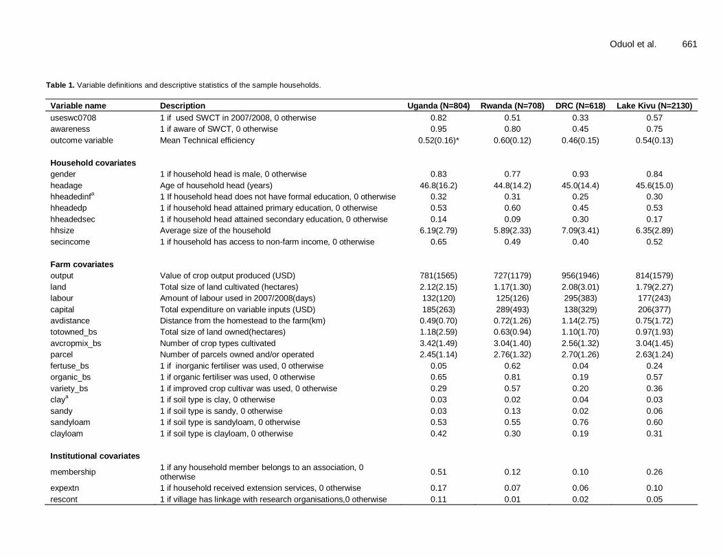
660 J. Dev. Agric. Econ. We have attempted to control for variations in TE due to differences in the quality of inputs by introducing dummy variables such as use of improved crop cultivars, organic fertilisers and inorganic fertilisers. Finally, given that the pooled production function was estimated using data from three different countries, which are likely to encounter differing bio-physical, socio-economic and institutional factors, we have included country dummies in the pooled model to capture the effects of the aforementioned variations on TE. Regional dummies have been used in other past studies to capture the effect of policy, climatic and other environmental factors (Kumbhakar et al., 1991). RESULTS AND DISCUSSION This section describes the results of the estimation of individual country and pooled frontiers. In addition, population impact parameters and the determinants of TE estimated for individual countries and the pooled sample using OLS and exponential NLS methods are presented and discussed. Characteristics of the sample households Table 1 presents descriptive statistics of the sample households. On average, household heads are 46 years old and 84% of them are male. Only 16% of the household heads attained at least secondary school level of education, whereas majority (53%) attained at most primary education.

The data indicate that the levels of awareness and adoption of SWC technologies vary by country. While the level of awareness is relatively high in Uganda (95%) and Rwanda (80%), only 45% of the households in the DRC are aware of the technologies. Adoption level is, however, considerably low in Rwanda (51%) and the DRC (33%) compared to Uganda (82%). The data on institutional variables suggest that most of the households have limited access to institutional services. For instances, only 6% and 34% of the households in the Lake Kivu PLS reside in villages that have linkages with organisations that conduct research and provide extension services respectively. The scenario is, however, different when the analysis is considered by country. In general, households in Rwanda and the DRC appear to have fewer institutional linkages than those in Uganda.

Farm level characteristics reveal that households in the Lake Kivu PLS own slightly less than one hectare of land, but the size of owned land ranges from 0.63 ha in Rwanda to 1.18 ha in Uganda. On the other hand, households cultivate an average of 1.8 ha of land in a year

6. On average, the households use 177 person-days

6 Given that the three countries in the Lake Kivu PLS have two seasons in a year, the average size of land under cultivation in a season is taken to be half of that reported for

the year. However, the size may be more or less than half of that cultivated in a year depending on the number of seasons the household cultivated the land.

of labour in a year, although the amount ranges from 132 to 295 person-days in Rwanda and the DRC, respectively. The results suggest that fewer households use improved inputs such as fertiliser and improved crop varieties in Uganda and the DRC than in Rwanda. The relatively higher levels of use of improved inputs in Rwanda can be attributed to supportive agricultural policies, such as the crop intensification programme, which have facilitated the acquisition and use of inorganic fertilisers and improved seeds through government subsidies. On average, value of crop output produced in the Lake Kivu PLS is US$814 and ranges from US$ 727 in Rwanda to US$956 in the DRC.

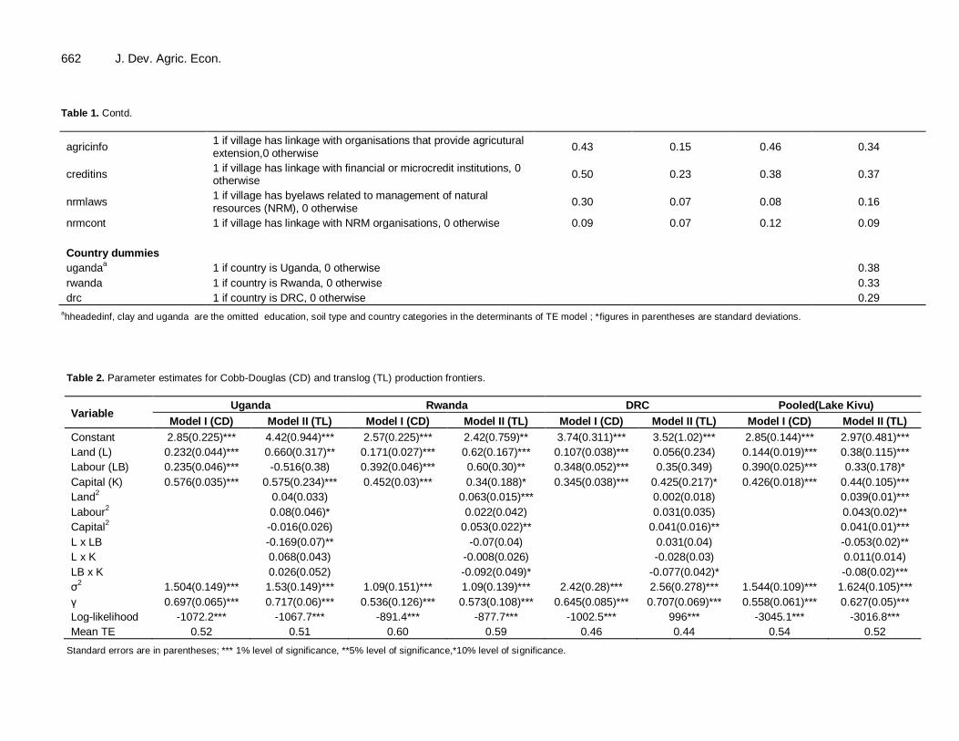
Technical efficiency Table 2 provides a summary of the Maximum Likelihood Estimation (MLE) coefficients for the Cobb-Douglas (CD) and translog (TL) stochastic frontier production functions

7. The values for the parameters and are

significant at 1%, thus indicating that the residual variation is due to technical inefficiency. The one-sided generalised likelihood ratio test of shows statistics that are sufficiently larger than the 5% critical value, suggesting that the traditional average response function is not an adequate representation of the data (that is, the stochastic and not the deterministic function is more appropriate for the datasets). We selected the Cobb-Douglas function as an adequate representation of the data for individual country and pooled frontiers based on the values of the one-sided generalised likelihood ratio tests, which are larger than those of the translog functions as indicated in Table 2.

Both individual country and pooled Cobb-Douglas models show that the coefficients associated with land, labour and capital are positive and statistically significant at 1%. Thus, the data suggest that the households could increase the value of output by increasing the amount of land, labour and capital. In Uganda, Rwanda and Lake Kivu, a larger increase in output would be realised if the households increased the levels of capital, while labour accounts for the largest variation in output in the DRC. Furthermore, the sum of the coefficients suggests that farmers in Rwanda and Uganda are operating under increasing returns to scale while those in the DRC are operating under decreasing returns to scale. The mean TE scores suggest that TE is lower in the DRC (46%) and Uganda (52%) than in Rwanda (60%). On average, mean

7 We estimated both the Cobb-Douglas and the translog stochastic production frontiers under the assumption of half-normal and truncated normal distribution and opted for the Cobb-Douglas function estimated under the half-normal distribution because we failed

to reject the hypothesis that the distribution is half-normal for the individual country frontiers (Appendix 1). In order to test for the appropriateness of the Cobb-Douglas model, we tested the following null and alternative hypotheses, H0:σ2 =0 versus alternative H1:σ2>0 and H0:γ =0 versus alternative H1:γ>0. The results of the one-sided

likelihood-ratio test that resulted in the rejection of the null hypotheses are provided in Table 2.

Oduol et al. 661 Table 1. Variable definitions and descriptive statistics of the sample households.

Variable name Description Uganda (N=804) Rwanda (N=708) DRC (N=618) Lake Kivu (N=2130)

useswc0708 1 if used SWCT in 2007/2008, 0 otherwise 0.82 0.51 0.33 0.57

awareness 1 if aware of SWCT, 0 otherwise 0.95 0.80 0.45 0.75

outcome variable Mean Technical efficiency 0.52(0.16)* 0.60(0.12) 0.46(0.15) 0.54(0.13)

Household covariates

gender 1 if household head is male, 0 otherwise 0.83 0.77 0.93 0.84

headage Age of household head (years) 46.8(16.2) 44.8(14.2) 45.0(14.4) 45.6(15.0)

hheadedinfa 1 If household head does not have formal education, 0 otherwise 0.32 0.31 0.25 0.30

hheadedp 1 if household head attained primary education, 0 otherwise 0.53 0.60 0.45 0.53

hheadedsec 1 if household head attained secondary education, 0 otherwise 0.14 0.09 0.30 0.17

hhsize Average size of the household 6.19(2.79) 5.89(2.33) 7.09(3.41) 6.35(2.89)

secincome 1 if household has access to non-farm income, 0 otherwise 0.65 0.49 0.40 0.52

Farm covariates

output Value of crop output produced (USD) 781(1565) 727(1179) 956(1946) 814(1579)

land Total size of land cultivated (hectares) 2.12(2.15) 1.17(1.30) 2.08(3.01) 1.79(2.27)

labour Amount of labour used in 2007/2008(days) 132(120) 125(126) 295(383) 177(243)

capital Total expenditure on variable inputs (USD) 185(263) 289(493) 138(329) 206(377)

avdistance Distance from the homestead to the farm(km) 0.49(0.70) 0.72(1.26) 1.14(2.75) 0.75(1.72)

totowned_bs Total size of land owned(hectares) 1.18(2.59) 0.63(0.94) 1.10(1.70) 0.97(1.93)

avcropmix_bs Number of crop types cultivated 3.42(1.49) 3.04(1.40) 2.56(1.32) 3.04(1.45)

parcel Number of parcels owned and/or operated 2.45(1.14) 2.76(1.32) 2.70(1.26) 2.63(1.24)

fertuse_bs 1 if inorganic fertiliser was used, 0 otherwise 0.05 0.62 0.04 0.24

organic_bs 1 if organic fertiliser was used, 0 otherwise 0.65 0.81 0.19 0.57

variety_bs 1 if improved crop cultivar was used, 0 otherwise 0.29 0.57 0.20 0.36

claya 1 if soil type is clay, 0 otherwise 0.03 0.02 0.04 0.03

sandy 1 if soil type is sandy, 0 otherwise 0.03 0.13 0.02 0.06

sandyloam 1 if soil type is sandyloam, 0 otherwise 0.53 0.55 0.76 0.60

clayloam 1 if soil type is clayloam, 0 otherwise 0.42 0.30 0.19 0.31

Institutional covariates

membership 1 if any household member belongs to an association, 0 otherwise

0.51 0.12 0.10 0.26

expextn 1 if household received extension services, 0 otherwise 0.17 0.07 0.06 0.10

rescont 1 if village has linkage with research organisations,0 otherwise 0.11 0.01 0.02 0.05

662 J. Dev. Agric. Econ. Table 1. Contd.

agricinfo 1 if village has linkage with organisations that provide agricutural extension,0 otherwise

0.43 0.15 0.46 0.34

creditins 1 if village has linkage with financial or microcredit institutions, 0 otherwise

0.50 0.23 0.38 0.37

nrmlaws 1 if village has byelaws related to management of natural resources (NRM), 0 otherwise

0.30 0.07 0.08 0.16

nrmcont 1 if village has linkage with NRM organisations, 0 otherwise 0.09 0.07 0.12 0.09

Country dummies

ugandaa 1 if country is Uganda, 0 otherwise 0.38

rwanda 1 if country is Rwanda, 0 otherwise 0.33

drc 1 if country is DRC, 0 otherwise 0.29 ahheadedinf, clay and uganda are the omitted education, soil type and country categories in the determinants of TE model ; *figures in parentheses are standard deviations.

Table 2. Parameter estimates for Cobb-Douglas (CD) and translog (TL) production frontiers.

Variable Uganda Rwanda DRC Pooled(Lake Kivu)

Model I (CD) Model II (TL) Model I (CD) Model II (TL) Model I (CD) Model II (TL) Model I (CD) Model II (TL)

Constant 2.85(0.225)*** 4.42(0.944)*** 2.57(0.225)*** 2.42(0.759)** 3.74(0.311)*** 3.52(1.02)*** 2.85(0.144)*** 2.97(0.481)***

Land (L) 0.232(0.044)*** 0.660(0.317)** 0.171(0.027)*** 0.62(0.167)*** 0.107(0.038)*** 0.056(0.234) 0.144(0.019)*** 0.38(0.115)***

Labour (LB) 0.235(0.046)*** -0.516(0.38) 0.392(0.046)*** 0.60(0.30)** 0.348(0.052)*** 0.35(0.349) 0.390(0.025)*** 0.33(0.178)*

Capital (K) 0.576(0.035)*** 0.575(0.234)*** 0.452(0.03)*** 0.34(0.188)* 0.345(0.038)*** 0.425(0.217)* 0.426(0.018)*** 0.44(0.105)***

Land2 0.04(0.033) 0.063(0.015)*** 0.002(0.018) 0.039(0.01)***

Labour2 0.08(0.046)* 0.022(0.042) 0.031(0.035) 0.043(0.02)**

Capital2 -0.016(0.026) 0.053(0.022)** 0.041(0.016)** 0.041(0.01)***

L x LB -0.169(0.07)** -0.07(0.04) 0.031(0.04) -0.053(0.02)**

L x K 0.068(0.043) -0.008(0.026) -0.028(0.03) 0.011(0.014)

LB x K 0.026(0.052) -0.092(0.049)* -0.077(0.042)* -0.08(0.02)***

σ2 1.504(0.149)*** 1.53(0.149)*** 1.09(0.151)*** 1.09(0.139)*** 2.42(0.28)*** 2.56(0.278)*** 1.544(0.109)*** 1.624(0.105)***

γ 0.697(0.065)*** 0.717(0.06)*** 0.536(0.126)*** 0.573(0.108)*** 0.645(0.085)*** 0.707(0.069)*** 0.558(0.061)*** 0.627(0.05)***

Log-likelihood -1072.2*** -1067.7*** -891.4*** -877.7*** -1002.5*** 996*** -3045.1*** -3016.8***

Mean TE 0.52 0.51 0.60 0.59 0.46 0.44 0.54 0.52

Standard errors are in parentheses; *** 1% level of significance, **5% level of significance,*10% level of significance.

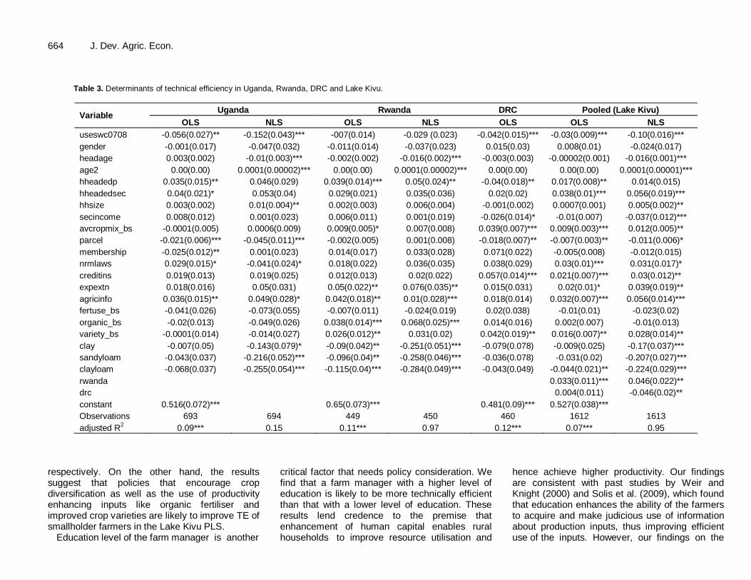
TE is estimated at 54% in the Lake Kivu PLS (pooled sample), indicating that the sample households can improve TE by 46% without necessarily altering the current levels of inputs. On the whole, the gains from improving TE appear to be much higher for households in the DRC and Uganda than in Rwanda. Determinants of technical efficiency A summary of the coefficient estimates for the determinants of technical efficiency is provided in Table 3

8. The results indicate a negative relationship between

adoption of SWC technologies and TE, although the magnitude of the effect varies by country and the model

9.

For instance, the effect is negative and significant for all the countries and the models except for Rwanda where the coefficient is negative but not significant. Besides, the exponential NLS models return coefficients for adoption of SWC technologies with greater magnitudes than those obtained from the OLS estimation. The results indicate that holding other factors constant under the assumption of homogeneous impact, adoption of SWC technologies is associated with a decrease of 6, 4 and 3% in TE on smallholder farms in Uganda, the DRC and Lake Kivu, respectively. However, when the impact is assumed to be heterogeneous, adoption of SWC technologies is associated with a 15 and 10% decline in TE in Uganda and Lake Kivu, respectively.

Apart from adoption of SWC technologies, the results suggest that institutional variables such as the existence of bylaws that regulate the use and management of natural resources, village linkage with organisations that provide agricultural extension and financial services and access to extension are significant determinants of TE, although the importance of the variables varies by country and model. In Uganda, for instance, farmers living in villages linked with institutions that provide extension are found to be more technically efficient than those living in villages with no such organisations. In Rwanda, however, village linkage with extension-based organisations and access to extension services are the most important determinants of TE among the institutional variables. In the DRC, households residing in villages that are linked with financial institutions are significantly more technically efficient than those living in villages with no linkages with credit institutions. These findings are corroborated by the descriptive results presented in Table 1, which suggest that institutional linkages in the Lake Kivu PLS are either lacking or weak, particularly in Rwanda and the DRC. The findings suggest that interventions that aim at improving technical

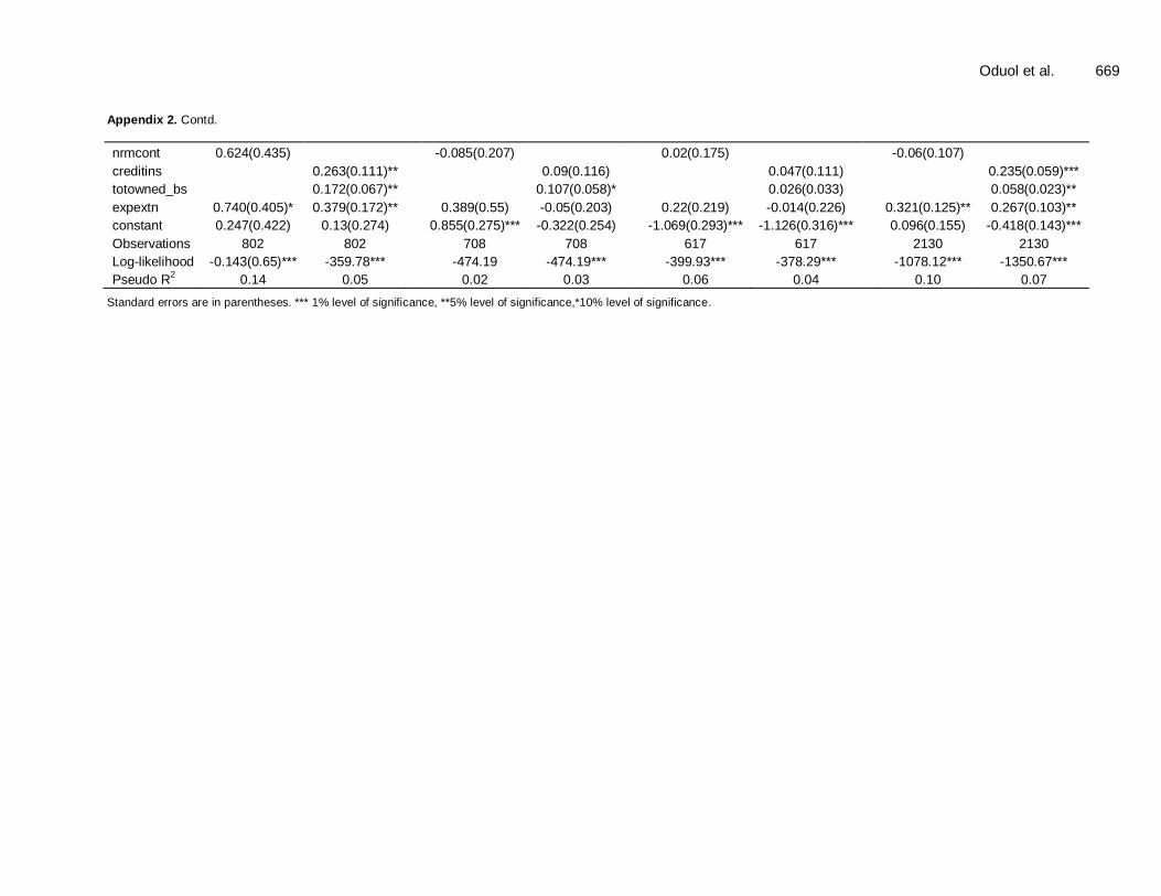
8 Since the focus of this paper is on impact of adoption of SWC technologies on technical efficiency, we have presented the estimated results for the determinants of awareness and adoption of SWC technologies in Appendix 2 in the appendix to allow sufficient space for the discussion of the key findings. 9 Note that the exponential NLS coefficients could not be estimated for the DRC because the model failed to converge.

Oduol et al. 663 efficiency in the three countries will need to focus on establishing and strengthening institutional linkages between farmers and institutions that provide extension and credit as well as grass root organisations that implement and enforce bylaws that govern the exploitation of natural resources. Our results bear out on other studies, which have shown that well-functioning institutions are prerequisites for enhanced agricultural productivity and efficiency (WDR, 2007). Well-functioning institutions are not only instrumental in internalising external factors that constrain adoption of improved technologies, but are a source of knowledge on appropriate productivity enhancing inputs. Indeed, well-functioning institutions have been documented to reduce transaction costs associated with the search for information on productivity enhancing inputs, credit and output markets, and thereby improving technical efficiency of smallholder farmers (Aryeetey et al., 1997; Jayne et al., 1997). Given that appropriate installation and maintenance of SWC structures require sufficient knowledge of the procedures, establishing linkages with extension-based organisations is likely to improve technical efficiency by enhancing the quality of SWC structures used by the farmers. This proposition is reinforced by Owuor and Ouma (2009)’s study which found that training in agriculture improves efficiency in resources use. Similarly, linkage with financial or microcredit institutions is likely to improve the farmers’ access to credit, thereby mitigating liquidity constraints associated with the installation of SWC structures. Thus, the results lend credence to our hypothesis that an approach to agricultural research and development that aims at establishing and strengthening institutional linkages between farmers and key stakeholders along the agricultural value chain such as IAR4D has the potential to improve TE of smallholder farmers in the three countries.

The country dummies in the pooled model indicate that households in Uganda are significantly less technically efficient than those in Rwanda but more technically efficient than households in the DRC. This finding can be attributed to the variation in the levels of use of conventional inputs among households in the three countries in addition to variations in biophysical and institutional factors. The levels of use of productivity enhancing inputs were found to be lower in the DRC than in Uganda but higher in Rwanda than in Uganda. In fact, the findings are reinforced by the coefficients for use of improved crop cultivars and organic fertilisers which are positive and significant in Rwanda but insignificant in DRC and Uganda. While the aforementioned institutional interventions are likely to improve technical efficiency of smallholder farmers in the Lake Kivu PLS, there is need to pay attention to other farm level covariates that are likely to negate the benefits of adoption of SWC technologies such as land fragmentation and labour availability as suggested by the significant coefficients for the number of parcels operated and household size

664 J. Dev. Agric. Econ.

Table 3. Determinants of technical efficiency in Uganda, Rwanda, DRC and Lake Kivu.

Variable Uganda Rwanda DRC Pooled (Lake Kivu)

OLS NLS OLS NLS OLS OLS NLS

useswc0708 -0.056(0.027)** -0.152(0.043)*** -007(0.014) -0.029 (0.023) -0.042(0.015)*** -0.03(0.009)*** -0.10(0.016)***

gender -0.001(0.017) -0.047(0.032) -0.011(0.014) -0.037(0.023) 0.015(0.03) 0.008(0.01) -0.024(0.017)

headage 0.003(0.002) -0.01(0.003)*** -0.002(0.002) -0.016(0.002)*** -0.003(0.003) -0.00002(0.001) -0.016(0.001)***

age2 0.00(0.00) 0.0001(0.00002)*** 0.00(0.00) 0.0001(0.00002)*** 0.00(0.00) 0.00(0.00) 0.0001(0.00001)***

hheadedp 0.035(0.015)** 0.046(0.029) 0.039(0.014)*** 0.05(0.024)** -0.04(0.018)** 0.017(0.008)** 0.014(0.015)

hheadedsec 0.04(0.021)* 0.053(0.04) 0.029(0.021) 0.035(0.036) 0.02(0.02) 0.038(0.01)*** 0.056(0.019)***

hhsize 0.003(0.002) 0.01(0.004)** 0.002(0.003) 0.006(0.004) -0.001(0.002) 0.0007(0.001) 0.005(0.002)**

secincome 0.008(0.012) 0.001(0.023) 0.006(0.011) 0.001(0.019) -0.026(0.014)* -0.01(0.007) -0.037(0.012)***

avcropmix_bs -0.0001(0.005) 0.0006(0.009) 0.009(0.005)* 0.007(0.008) 0.039(0.007)*** 0.009(0.003)*** 0.012(0.005)**

parcel -0.021(0.006)*** -0.045(0.011)*** -0.002(0.005) 0.001(0.008) -0.018(0.007)** -0.007(0.003)** -0.011(0.006)*

membership -0.025(0.012)** 0.001(0.023) 0.014(0.017) 0.033(0.028) 0.071(0.022) -0.005(0.008) -0.012(0.015)

nrmlaws 0.029(0.015)* -0.041(0.024)* 0.018(0.022) 0.036(0.035) 0.038(0.029) 0.03(0.01)*** 0.031(0.017)*

creditins 0.019(0.013) 0.019(0.025) 0.012(0.013) 0.02(0.022) 0.057(0.014)*** 0.021(0.007)*** 0.03(0.012)**

expextn 0.018(0.016) 0.05(0.031) 0.05(0.022)** 0.076(0.035)** 0.015(0.031) 0.02(0.01)* 0.039(0.019)**

agricinfo 0.036(0.015)** 0.049(0.028)* 0.042(0.018)** 0.01(0.028)*** 0.018(0.014) 0.032(0.007)*** 0.056(0.014)***

fertuse_bs -0.041(0.026) -0.073(0.055) -0.007(0.011) -0.024(0.019) 0.02(0.038) -0.01(0.01) -0.023(0.02)

organic_bs -0.02(0.013) -0.049(0.026) 0.038(0.014)*** 0.068(0.025)*** 0.014(0.016) 0.002(0.007) -0.01(0.013)

variety_bs -0.0001(0.014) -0.014(0.027) 0.026(0.012)** 0.031(0.02) 0.042(0.019)** 0.016(0.007)** 0.028(0.014)**

clay -0.007(0.05) -0.143(0.079)* -0.09(0.042)** -0.251(0.051)*** -0.079(0.078) -0.009(0.025) -0.17(0.037)***

sandyloam -0.043(0.037) -0.216(0.052)*** -0.096(0.04)** -0.258(0.046)*** -0.036(0.078) -0.031(0.02) -0.207(0.027)***

clayloam -0.068(0.037) -0.255(0.054)*** -0.115(0.04)*** -0.284(0.049)*** -0.043(0.049) -0.044(0.021)** -0.224(0.029)***

rwanda

0.033(0.011)*** 0.046(0.022)**

drc

0.004(0.011) -0.046(0.02)**

constant 0.516(0.072)***

0.65(0.073)***

0.481(0.09)*** 0.527(0.038)***

Observations 693 694 449 450 460 1612 1613

adjusted R2 0.09*** 0.15 0.11*** 0.97 0.12*** 0.07*** 0.95

respectively. On the other hand, the results suggest that policies that encourage crop diversification as well as the use of productivity enhancing inputs like organic fertiliser and improved crop varieties are likely to improve TE of smallholder farmers in the Lake Kivu PLS.

Education level of the farm manager is another

critical factor that needs policy consideration. We find that a farm manager with a higher level of education is likely to be more technically efficient than that with a lower level of education. These results lend credence to the premise that enhancement of human capital enables rural households to improve resource utilisation and

hence achieve higher productivity. Our findings are consistent with past studies by Weir and Knight (2000) and Solis et al. (2009), which found that education enhances the ability of the farmers to acquire and make judicious use of information about production inputs, thus improving efficient use of the inputs. However, our findings on the

Oduol et al. 665

Table 4. Estimated population impact parameters.

Parameter Uganda Rwanda DRC

Pooled (Lake Kivu)

OLS NLS OLS NLS OLS OLS NLS

No. of observations 802 802 708 708 617 2130 2130

No. with instrument(aware) 759 759 564 564 277 1603 1603

No treated( adopters) 657 657 359 359 206 1224 1224

LARF (Late) -0.06(0.03)* -0.09(0.03)*** -0.007(0.02) -0.02(0.02) -0.04 (0.03) -0.03(0.01)** -0.05 (0.02)***

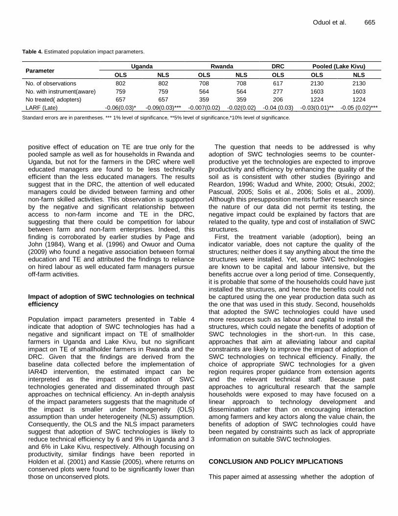
Standard errors are in parentheses. *** 1% level of significance, **5% level of significance,*10% level of significance. positive effect of education on TE are true only for the pooled sample as well as for households in Rwanda and Uganda, but not for the farmers in the DRC where well educated managers are found to be less technically efficient than the less educated managers. The results suggest that in the DRC, the attention of well educated managers could be divided between farming and other non-farm skilled activities. This observation is supported by the negative and significant relationship between access to non-farm income and TE in the DRC, suggesting that there could be competition for labour between farm and non-farm enterprises. Indeed, this finding is corroborated by earlier studies by Page and John (1984), Wang et al. (1996) and Owuor and Ouma (2009) who found a negative association between formal education and TE and attributed the findings to reliance on hired labour as well educated farm managers pursue off-farm activities. Impact of adoption of SWC technologies on technical efficiency Population impact parameters presented in Table 4 indicate that adoption of SWC technologies has had a negative and significant impact on TE of smallholder farmers in Uganda and Lake Kivu, but no significant impact on TE of smallholder farmers in Rwanda and the DRC. Given that the findings are derived from the baseline data collected before the implementation of IAR4D intervention, the estimated impact can be interpreted as the impact of adoption of SWC technologies generated and disseminated through past approaches on technical efficiency. An in-depth analysis of the impact parameters suggests that the magnitude of the impact is smaller under homogeneity (OLS) assumption than under heterogeneity (NLS) assumption. Consequently, the OLS and the NLS impact parameters suggest that adoption of SWC technologies is likely to reduce technical efficiency by 6 and 9% in Uganda and 3 and 6% in Lake Kivu, respectively. Although focusing on productivity, similar findings have been reported in Holden et al. (2001) and Kassie (2005), where returns on conserved plots were found to be significantly lower than those on unconserved plots.

The question that needs to be addressed is why adoption of SWC technologies seems to be counter-productive yet the technologies are expected to improve productivity and efficiency by enhancing the quality of the soil as is consistent with other studies (Byiringo and Reardon, 1996; Wadud and White, 2000; Otsuki, 2002; Pascual, 2005; Solis et al., 2006; Solis et al., 2009). Although this presupposition merits further research since the nature of our data did not permit its testing, the negative impact could be explained by factors that are related to the quality, type and cost of installation of SWC structures.

First, the treatment variable (adoption), being an indicator variable, does not capture the quality of the structures; neither does it say anything about the time the structures were installed. Yet, some SWC technologies are known to be capital and labour intensive, but the benefits accrue over a long period of time. Consequently, it is probable that some of the households could have just installed the structures, and hence the benefits could not be captured using the one year production data such as the one that was used in this study. Second, households that adopted the SWC technologies could have used more resources such as labour and capital to install the structures, which could negate the benefits of adoption of SWC technologies in the short-run. In this case, approaches that aim at alleviating labour and capital constraints are likely to improve the impact of adoption of SWC technologies on technical efficiency. Finally, the choice of appropriate SWC technologies for a given region requires proper guidance from extension agents and the relevant technical staff. Because past approaches to agricultural research that the sample households were exposed to may have focused on a linear approach to technology development and dissemination rather than on encouraging interaction among farmers and key actors along the value chain, the benefits of adoption of SWC technologies could have been negated by constraints such as lack of appropriate information on suitable SWC technologies. CONCLUSION AND POLICY IMPLICATIONS This paper aimed at assessing whether the adoption of

666 J. Dev. Agric. Econ. soil and water conservation (SWC) technologies generated and disseminated before the implementation of IAR4D has had an impact on technical efficiency (TE) of smallholder farmers in Uganda, Rwanda and the DRC. In addition, the paper focused on examining the potential effectiveness of IAR4D on improving technical efficiency of smallholder farmers through the establishment and strengthening of institutional linkages among smallholder farmers and key stakeholders along the agricultural value chain.

First, we estimated individual country and pooled Cobb Douglas production frontiers and found that on average the sample households in Rwanda, Uganda the DRC could increase technical efficiency by 40, 48 and 54%, respectively without necessarily altering the existing level of inputs. Second, the TE scores were regressed on adoption of SWC technologies while controlling for other household, farm level and institutional covariates to identify the determinants of TE as well as to quantify the impact of adoption of SWC technologies on technical efficiency. In this case, instrumental variable approach was adopted to estimate local average treatment effect (LATE) using both ordinary least squares (OLS) and weighted non-linear least squares (NLS) method.

Three main empirical findings emerge from this study. First, we find that adoption of SWC technologies is negative and significantly associated with TE in Uganda, the DRC and in the Lake Kivu PLS (pooled sample), suggesting that the benefits of adoption of SWC technologies have not been translated into improved TE in the Lake Kivu region. The findings, therefore, suggest that interventions that aim at improving technical efficiency of the sample households should focus on alleviating constraints associated with the use of SWC technologies. The factors that are likely to explain the negative relationship, but need to be corroborated with empirical evidence from further research are the effect of the quality of SWC structures as well as the cost of installation of the structures.

Second, the positive and significant relationship between TE and institutional variables such as the presence of bylaws that govern the use and management of natural resources, linkage with extension-based organisations and financial institutions and access to extension services suggest that an approach to agricultural research and development that aims at establishing and strengthening institutional linkages between farmers and key stakeholders along the agricultural value chain such as IAR4D has the potential to improve technical efficiency of smallholder farmers in the three countries. However, while recognising significant effects of institutional linkages in improving TE, special attention needs to be paid to farm level factors such as use of improved inputs, crop diversification and land-fragmentation as well as household covariates like education level of the farm managers. Those factors that enhance efforts geared towards improving efficiency

outcomes need to be fostered while those that jeopardise the efforts require mitigation.

Finally, it can be deduced from the findings that adoption of SWC technologies generated and disseminated through past approaches to agricultural research and development have not improved technical efficiency of smallholder farmers in the Lake Kivu PLS. Instead, adoption of SWC technologies appears to be counter-productive for smallholder farmers in the Lake Kivu PLS. While further research is necessary to examine factors that negate the benefits of adoption of SWC technologies among the sample households, one major implication that stems from the findings of this study is that there is an urgent need for an approach to agricultural research and development that is likely to tailor the technologies to the needs of smallholder farmers and internalise external factors that jeopardise the farmers’ efforts towards reaching the production frontier.

REFERENCES

Abadie A (2003). ‘Semiparametric instrumental variable estimation of treatment response models’. Econom. J., 113: 231-263.

Angrist JD, Imbens GW (1991). Identification and estimation of local

average treatment effects. Technical Working Paper No. 118. Angrist JD, Imbens GW, Rubin DB (1996). ‘Identification of causal

effects using instrumental variables’. Am. J. Stat. Assoc., 91: 444-

472. Aryeetey E, Hettige H, Nissanke M, Steel W (1997). Financial market

and reforms in sub-Saharan Africa.World Bank Technical Paper No.

356, Washington, D.C. Battese GE, Coelli TJ (1995). ‘A model for technical inefficiency effects

in a stochastic frontier production function for panel data’. Empir. Econ., 20: 325-332.

Byiringo F, Reardon T (1996). ‘Farm productivity in Rwanda: effects of farm size, erosion, and soil conservation investments’. J. Agric. Econ.

15:127-136. Cameron AC, Trivedi PK (2005). Microeconometrics: Methods and

Applications. Cambridge University Press, New York.

Coelli TJ, Rao DSP, Battese GE (1998). An Introduction to Efficiency and Productivity Analysis. Kluwer Academic Publishers, Boston.

Diagne A, Sogbossi MJ, Simtowe F (2009). Estimation of actual and

potential adoption rates and determinants of a new technology not universally known in the population: The case of NERICA rice varieties in Guinea. Contributor paper 354 to the International

Association of Agricultural Economists Conference, August 16-22, 2009, Beijing, China.

Drechsel P, Olaleye A, Adeoti A, Thiombiano L, Barry B, Vohland K

(2005). Adoption driver and constraints of resource conservation technologies in sub-Saharan Africa, Institute of Water Management. www.westafrica2.iwmi.org/pdf/AdoptionConstraints-Overview.pdf

[June 2010]. FARA (2005). LKPLS validation report 2003. Forum for Agricultural

Research in Africa Sub-Saharan Africa Challenge Program. Findings

of the Lake Kivu Pilot Learning Site Validation Team: A Mission Undertaken to Identify Key Entry Points for Agricultural Research and Rural Enterprise Development in East and Central Africa.

Farrell MJ (1957). ‘The measurement of productive efficiency’. J. Royal Stat. Soc. 3:253-290.

Farrow A, Opondo C, Tenywa M, Rao KPC, Nkonya E, Njeru R,

Lubanga L (2009). Selecting sites to prove the concept of integrated research for agricultural development: LKPL Site selection annual report (2008/9).

Forum for Agricultural Research in Africa (2008) Medium-Term Plan 2009-2010, Sub-Saharan Africa Challenge Programme.

Hayami Y, Ruttan WV (1985). Agricultural Development: An

International Perspective. The Johns Hopkins University Press, Baltimore and London.

Heckman J, Vytlacil E (2005). ‘Structural equations, treatment effect, and econometrics policy evaluation’. Econometrica, 73: 669-738.

Heckman JJ (1990). ‘Varieties of selection bias’. Am. Econ. Rev., 80:

313-318. Heckman JJ, Robb R (1985). ‘Alternative methods for evaluating the

impact of interventions’ in Heckman JJ, Singer B (eds), Longitudinal

Analysis of Labor Market Data. Cambridge University Press, New

York. Holden S, Shiferaw B, Pender J (2001). ‘Market imperfections and land

productivity in Ethiopian highlands’. J. Agric. Econ., 52: 53-70. Imbens GW, Angrist JD (1994). ‘Identification and estimation of local

average treatment effects’. Econometrica, 62: 467-475.

Imbens GW, Wooldridge J (2009). ‘Recent Developments in the Econometrics of Programme Evaluation’. J. Econ. Lit., 47: 5-86.

Jayne T, Shaffer J, Staatz J, Reardon T (1997). Improving the impact of

market reform on agricultural productivity in Africa: How institutional design makes a difference. East Lansing, MI: Michigan State University.

Jayne TS, Mather D, Mghenyi E (2006). Smallholder farming under increasingly difficult circumstances: policy and public investment priorities for Africa, Food Security International Development Policy

Syntheses 54507, Michigan State University, Department of Agricultural, Food, and Resource Economics, www.aec.msu.edu/fs2/papers/idwp86.pdf [July 2008].

Kassie M (2005). Technology adoption, land rental contracts and agricultural productivity, PhD dissertation, Norwegian University of Life Sciences.

Kumbhakar SC, Ghosh S, McGuckin JT (1991). ‘A generalized production frontier approach for estimating determinants of inefficiency in U.S. Dairy Farms’. J. Bus. Econ. Stat., 9: 279-286

Lee MJ (2005). Microeconometrics for Policy, Program and Treatment Effects. Advanced Text in Econometrics, Oxford University Press.

Loeffen M, Ndjeunga J, Kelly V, Sylla ML, Traore B, Tessougue M

(2008). Uptake of soil and water conservation technologies in West Africa: A Case Study of the Office de la Haute Vallée du Niger (OHVN) in Mali, www.icrisat.org/what-we-do/impi/whats-

new/WPS%2025-1092.pdf [June 2010]. Lovell CAK (1993). ‘Production frontiers and productive efficiency’ in

Fried HO, Lovell CAK, Schmidt SS (eds.), The Measurement of

Productive Efficiency: Techniques and Applications. Oxford University Press Inc., New York.

McCulloch AK, Meinzen-Dick R, Hazell P (1998). Property rights,

collective action and Technologies for Natural Resource Management: A Conceptual Framework. IFPRI SP-PRCA Working

Paper No. 1. Ndjeunga J, Bantilan MCS (2005). ‘Uptake of improved technologies in

the Semi-arid Tropics of West Africa: Why is agricultural transformation lagging behind?’ J. Agric. Dev. Econ., 2: 85-102.

Oehmke JF, Crawford EW (1996). ‘The impact of agricultural

technology in sub-Saharan Afr. J. Afr. Econ., 5: 271-292.

Otsuki K, Hardie I, E. Reis E (2002). ‘The implication of property rights for joint agriculture–timber productivity in the Brazilian Amazon’. Environ. Dev. Econ., 7: 299-323.

Owuor G, Ouma SA (2009). What are the key constraints in technical

efficiency of smallholder farmers in Africa: evidence from Kenya. A paper presented at the 111 EAAE-IAAE Seminar ‘Small Farms: decline or persistence’ University of Kent, Canterbury, UK, 26

th-27

th

June 2009. Page MJ, John M (1984). Firm Size and Technical Efficiency:

applications of production frontiers to Indian survey data. J. Dev.

Econ., 16: 29-52. Pascual U (2005). Land use intensification potential in slash-and-burn

farming through improvements in technical efficiency. Ecol. Econ.,

52: 497-511.

Oduol et al. 667 Pender J, Jagger P, Nkonya E, Sserunkuuma D (2001). Development

pathways and land management in Uganda: causes and implications. International Food Policy Research Institute (IFPRI), Environment

and Production Technology Division (EPTD) Discussion Paper No.85 Ravallion M (2001). The mystery of the vanishing benefits: an

introduction to impact evaluation. World Bank Econ. Rev., 15: 115-

140. Ray SC (2004). Data Envelopment Analysis: Theory and Techniques for

Economics and Operation Research. Cambridge University Press,

New York. Reardon T, Kelly V, Jayne T, Savadogo K, Clay D (1996). Determinants

of farm productivity in Africa: a synthesis of four case studies,

Department of Agricultural Economics and the Department of Economics, Michigan State Lansing, Michigan, U.S.A., www. msu.edu/agecon/fs2/papers.pdf [2010, June].

Renkow M, Byerlee D (2010). ‘The Impacts of CGIAR Research: A Review of Recent Evidence’. J. Food Pol. (in press).

Roehrig CS (1988). Conditions for identification in nonparametric and

parametric models. Econometrica, 56: 433-447. Rubin DB (1974). ‘Estimating causal effects of treatments in

randomized and nonrandomized studies. J. Educ. Psychol., 66: 688-

701. Rubin DB (1977). ‘Assignment to treatment group on the basis of a

covariate’. J. Educ. Stat., 2: 1-26.

Scherr SJ (1999). Soil degradation: A threat to developing-country food security by 2020? IFPRI, Food, Agriculture and The Environment Discussion Paper No. 27.

Sidibé A (2005). Farm-level adoption of soil and water conservation techniques in Northern Burkina Faso’. Agr. Water Manag., 71:211-224.

Smaling EAM, Nandwa SM, Jansen BH (1997). ‘Soil fertility in Africa is at stake’ in Buresh RJ, Sanchez P, Calhoun F (eds.), Replenishing Soil Fertility in Africa, Special publication, USA: Madison, pp. 64-81.

Solis D, Bravo-Ureta B, Quiroga ER (2006). Technical efficiency and adoption of soil conservation in El Salvador and Honduras. Contributed paper prepared for presentation at the International

Association of Agricultural Economists Conference, Gold Coast, Australia, August 12-18, 2006.

Solis D, Bravo-Ureta B, Quiroga ER (2009). ‘Technical efficiency among

peasant farmers participating in Natural Resource Management Programmes in Central America’. J. Agric. Econ., 60: 202-219.

Wadud A, White B (2000). Farm household efficiency in Bangladesh: a

comparison of stochastic frontier and DEA methods. J. Appl. Econ., 32: 1665-1673.

Wang J, Eric JW, Gail LC (1996). ‘A Shadow-price frontier

measurement of profit efficiency in Chinese agriculture’. Am. J. Agric. Econ., 78: 146-156.

Weir S, Knight J (2000). Education externalities in rural Ethiopia. evidence from average and stochastic frontier production functions,

Working paper CSAEWPS/2000-4, Centre for the Study of African Economies, University of Oxford.

World Bank (2007). Agriculture for Development. World Development

Report 2008. Washington, DC. Zhu J (2003). Quantitative Models for Performance Evaluation and

Benchmarking: Data Envelopment Analysis with Spreadsheets and

Excel Solver. Kluwer Academic Publishers, Boston.

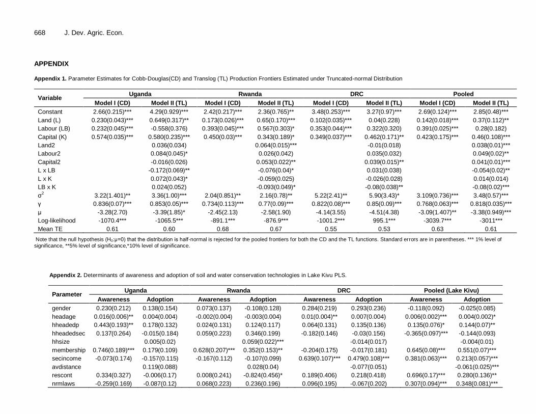
668 J. Dev. Agric. Econ. APPENDIX Appendix 1. Parameter Estimates for Cobb-Douglas(CD) and Translog (TL) Production Frontiers Estimated under Truncated-normal Distribution

Variable Uganda Rwanda DRC Pooled

Model I (CD) Model II (TL) Model I (CD) Model II (TL) Model I (CD) Model II (TL) Model I (CD) Model II (TL)

Constant 2.66(0.215)*** 4.29(0.929)*** 2.42(0.217)*** 2.36(0.765)** 3.48(0.253)*** 3.27(0.97)*** 2.69(0.124)*** 2.85(0.48)***

Land (L) 0.230(0.043)*** 0.649(0.317)** 0.173(0.026)*** 0.65(0.170)*** 0.102(0.035)*** 0.04(0.228) 0.142(0.018)*** 0.37(0.112)**

Labour (LB) 0.232(0.045)*** -0.558(0.376) 0.393(0.045)*** 0.567(0.303)* 0.353(0.044)*** 0.322(0.320) 0.391(0.025)*** 0.28(0.182)

Capital (K) 0.574(0.035)*** 0.580(0.235)*** 0.450(0.03)*** 0.343(0.189)* 0.349(0.037)*** 0.462(0.171)** 0.423(0.175)*** 0.46(0.108)***

Land2 0.036(0.034) 0.064(0.015)*** -0.01(0.018) 0.038(0.01)***

Labour2 0.084(0.045)* 0.026(0.042) 0.035(0.032) 0.049(0.02)**

Capital2 -0.016(0.026) 0.053(0.022)** 0.039(0.015)** 0.041(0.01)***

L x LB -0.172(0.069)** -0.076(0.04)* 0.031(0.038) -0.054(0.02)**

L x K 0.072(0.043)* -0.059(0.025) -0.026(0.028) 0.014(0.014)

LB x K 0.024(0.052) -0.093(0.049)* -0.08(0.038)** -0.08(0.02)***

σ2 3.22(1.401)** 3.36(1.00)*** 2.04(0.851)** 2.16(0.78)** 5.22(2.41)** 5.90(3.43)* 3.109(0.736)*** 3.48(0.57)***

γ 0.836(0.07)*** 0.853(0.05)*** 0.734(0.113)*** 0.77(0.09)*** 0.822(0.08)*** 0.85(0.09)*** 0.768(0.063)*** 0.818(0.035)***

μ -3.28(2.70) -3.39(1.85)* -2.45(2.13) -2.58(1.90) -4.14(3.55) -4.51(4.38) -3.09(1.407)** -3.38(0.949)***

Log-likelihood -1070.4*** -1065.5*** -891.1*** -876.9*** -1001.2*** 995.1*** -3039.7*** -3011***

Mean TE 0.61 0.60 0.68 0.67 0.55 0.53 0.63 0.61

Note that the null hypothesis (H0:μ=0) that the distribution is half-normal is rejected for the pooled frontiers for both the CD and the TL functions. Standard errors are in parentheses. *** 1% level of

significance, **5% level of significance,*10% level of significance.

Appendix 2. Determinants of awareness and adoption of soil and water conservation technologies in Lake Kivu PLS.

Parameter Uganda Rwanda DRC Pooled (Lake Kivu)

Awareness Adoption Awareness Adoption Awareness Adoption Awareness Adoption

gender 0.230(0.212) 0.138(0.154) 0.073(0.137) -0.108(0.128) 0.284(0.219) 0.293(0.236) -0.118(0.092) -0.025(0.085)

headage 0.016(0.006)** 0.004(0.004) -0.002(0.004) -0.003(0.004) 0.01(0.004)** 0.007(0.004) 0.006(0.002)*** 0.004(0.002)*

hheadedp 0.443(0.193)** 0.178(0.132) 0.024(0.131) 0.124(0.117) 0.064(0.131) 0.135(0.136) 0.135(0.076)* 0.144(0.07)**

hheadedsec 0.137(0.264) -0.015(0.184) 0.059(0.223) 0.346(0.199) -0.182(0.146) -0.03(0.156) -0.365(0.097)*** -0.144(0.093)

hhsize

0.005(0.02)

0.059(0.022)***

-0.014(0.017)

-0.004(0.01)

membership 0.746(0.189)*** 0.179(0.109) 0.628(0.207)*** 0.352(0.153)** -0.204(0.175) -0.017(0.181) 0.645(0.08)*** 0.551(0.07)***

secincome -0.073(0.174) -0.157(0.115) -0.167(0.112) -0.107(0.099) 0.639(0.107)*** 0.479(0.108)*** 0.381(0.063)*** 0.213(0.057)***

avdistance

0.119(0.088)

0.028(0.04)

-0.077(0.051)

-0.061(0.025)***

rescont 0.334(0.327) -0.006(0.17) 0.008(0.241) -0.824(0.456)* 0.189(0.406) 0.218(0.418) 0.696(0.17)*** 0.280(0.136)**

nrmlaws -0.259(0.169) -0.087(0.12) 0.068(0.223) 0.236(0.196) 0.096(0.195) -0.067(0.202) 0.307(0.094)*** 0.348(0.081)***

Oduol et al. 669

Appendix 2. Contd.

nrmcont 0.624(0.435)

-0.085(0.207)

0.02(0.175)

-0.06(0.107)

creditins

0.263(0.111)**

0.09(0.116)

0.047(0.111)

0.235(0.059)***

totowned_bs

0.172(0.067)**

0.107(0.058)*

0.026(0.033)

0.058(0.023)**

expextn 0.740(0.405)* 0.379(0.172)** 0.389(0.55) -0.05(0.203) 0.22(0.219) -0.014(0.226) 0.321(0.125)** 0.267(0.103)**

constant 0.247(0.422) 0.13(0.274) 0.855(0.275)*** -0.322(0.254) -1.069(0.293)*** -1.126(0.316)*** 0.096(0.155) -0.418(0.143)***

Observations 802 802 708 708 617 617 2130 2130

Log-likelihood -0.143(0.65)*** -359.78*** -474.19 -474.19*** -399.93*** -378.29*** -1078.12*** -1350.67***

Pseudo R2 0.14 0.05 0.02 0.03 0.06 0.04 0.10 0.07

Standard errors are in parentheses. *** 1% level of significance, **5% level of significance,*10% level of significance.