Page 1

Electronic Annex A: Data repository 1

Depth (cm)

Dissolved Mo nmol kg-1

Particulate Mo nmol kg-1

Total Mo nmol kg-1

Control nmol kg-1

June 2006 3.1 14.3 - 13.9 - 7.1 14.3 - 14.4 - 9.1 14.9 - 14.9 -

10.1 14.1 - 15.7 - 10.35 13.2 - 15.4 - 10.6 13.1 - 15.1 -

10.85 12.9 - 14.2 - 11.1 12.4 - 13.9 -

11.35 12.2 - 13.0 - 11.6 11.8 - 14.7 -

11.85 11.3 - 12.0 - 12.1 10.9 - 12.6 -

12.35 10.5 - 12.0 - 12.6 10.1 - 11.7 -

12.85 9.6 - 11.7 - 13.1 9.2 - 11.0 - 14.1 8.8 - 11.5 - 15.1 8.7 - 11.4 - 16.1 8.7 - 11.6 - 17.1 8.6 - 11.5 - 18.1 8.6 - 11.9 - 19.1 8.5 - 11.3 -

September 2006

1.4 13.0 0.4 13.9 13.4 3.4 14.4 0.2 15.4 14.6 7.4 14.7 0.2 14.7 14.9 9.9 15.2 0.3 12.5 15.5

10.4 13.9 0.3 11.7 14.2 10.9 14.2 0.2 11.8 14.4

11.15 11.7 0.7 11.4 12.4 11.4 11.3 0.6 10.0 11.8

11.65 13.3 2.0 8.3 15.3 11.9 8.1 2.3 8.2 10.3

12.15 6.2 2.3 7.7 8.5 12.4 6.2 2.4 8.0 8.6

12.65 6.4 3.2 7.6 9.6 12.9 7.0 2.2 7.5 9.2

13.15 6.9 1.7 7.8 8.5 13.4 5.6 2.7 7.5 8.3 13.9 5.2 1.7 6.6 6.9 14.4 4.5 3.8 6.9 8.3 15.4 4.0 2.7 6.7 6.7 16.4 3.6 3.2 6.2 6.8 17.4 4.1 3.6 6.2 7.6 18.4 3.3 3.6 6.1 6.9 19.4 3.9 3.8 6.9 7.6

August 2007

3.0 11.5 0.0 10.6 11.5 6.0 12.3 0.0 11.0 12.3 7.0 12.2 0.0 11.4 12.2

Page 2

8.0 13.1 0.0 12.5 13.1 8.5 12.8 0.0 12.7 12.8 9.0 14.1 0.0 13.2 14.1 9.5 12.3 0.0 12.1 12.3

10.0 11.7 0.2 10.6 11.9 10.5 10.7 0.5 7.3 11.2 11.0 7.2 0.7 4.8 7.9 11.5 3.6 1.9 5.0 5.5 12.0 2.2 2.4 3.9 4.6 12.5 2.7 2.0 4.1 4.7 13.0 2.3 2.0 3.6 4.3 15.0 2.9 1.8 4.1 4.7 17.0 2.9 2.0 3.3 4.9 19.0 1.8 2.4 4.0 4.3

2 Table A1: Molybdenum concentrations in filtered water (dissolved), unfiltered water (total) and on the 3

filter (particulate) for three different field trips. The relation [Mo]total = [Mo]dissolved + [Mo]particulate holds 4

within the precision of the analysis (no blank substraction). Standard reproducibility of the 5

measurement is 6.7% (2 s.d.). 6

7

Name Depth (cm)

[Μο] µmol kg-1-

LCAc1_pw1 0.0 23 LCAc1_pw2 1.5 214 LCAc1_pw3 3.0 158 LCAc1_pw4 4.5 204 LCAc1_pw5 6.0 355 LCAc1_pw6 7.5 234 LCAc1_pw7 9.0 192 LCAc1_pw8 10.5 253 LCAc1_pw9 12.1 109

LCAc1_pw10 13.6 405 LCAc1_pw11 15.1 1248 LCAc1_pw12 16.6 1592 LCAc1_pw13 18.1 1858 LCAc1_pw14 19.6 1301 LCAc1_pw15 21.1 751 LCAc1_pw16 22.6 431 LCAc1_pw17 24.1 4052 LCAc1_pw18 25.6 4248 LCAc1_pw19 27.1 313 LCAc1_pw20 28.6 1380 LCAc1_pw21 30.1 1739

Table A.2.: Pore fluid Mo concentrations for core 1 sampled at 21 m depth in August 2007. 8

9

Page 3

Date Total Mo Dissolved Mo Particulate Mo

Total Mo inventory

June 2006 36.2 33.7 2.5

September 2006 31.1 30.1 1.8

August 2007 22.5 23.5 1.0

Average ± sd 29.8±7.0 29.1±5.2 1.8±0.7

Mo inventory in the monimolimnion

June 2006 7.4 5.7 1.7

September 2006 3.6 3.0 1.3

August 2007 2.5 2.2 1.0

Average ± sd 4.5±2.6 3.6±1.8 1.3±0.3

10

Table A.3: Cumulative Mo inventories in Lake Cadagno (moles). Numbers are derived by stepwise 11

integration of the product between the water exchange area profile (DEL DON et al., 2001), and the 12

observed Mo profiles. For total particulate Mo, we integrate the observed particulate Mo profile and in 13

the case of June 2006 where particulate Mo has not been directly measured, we use particulate = total – 14

dissolved. For September 2006 and August 2007 the particulate profile was used in the integration 15

without blank correction, hence particulate Mo + dissolved Mo appears slightly greater than total Mo. 16

Importantly, the average values confirm mass balance within error. 17

18

Page 4

Electronic Annex B: Ground water flux. Eddy diffusion coefficient and subaquatic water and Mo 18 flux 19 20

The waters in Lake Cadagno are strongly influenced by a subaquatic supply of water. This solute rich 21

stream is sourced in dolomitic limestone. We show this based on Sr sources of dolomites from outcrops 22

near the lake (Fig. B1). Correlation of 1/[Sr] and 87Sr/86Sr in the water column in June 2006 (fitted line, 23

R2 = 0.96) and September 2006 (R2 =0.97) confirms that Sr behaves conservatively in the water 24

column. The water column Sr isotopic compositions defines a mixing line with the unradiogenic 25

dolomite end member and a mixture of dilute, radiogenic Sr from the river and swamps (inserted 26

panel). The standard reproducibility of the isotope measurements is similar or smaller than the size of 27

the symbols. 28

29

Figure B1: Water source characteristics in the lake. Sr behaves conservatively and lake waters contain 30

Sr mixed of primarily two sources; unradiogenic subaquatic springs (sourced in dolomite) and 31

radiogenic Sr from rivers/swamps (presumable sourced in older granites). 32

33

In contrast to Sr, molybdenum behaves non-conservatively in the water column. This is evident from 34

plots of δ98/95Mo versus 87Sr/86Sr, where the isotopes compositions are clearly decoupled around the 35

chemocline. 36

Page 5

37

38

Figure B2: δ98/95Mo versus 87Sr/86Sr in the water column a) June 2006, b) September 2006 and c) 39

August 2007. Sulfidic and oxic waters are marked with grey and black symbols, respectively. Note the 40

different y-scale in September 2006. We have derived 87Sr/86Sr values in August 2007 from the 41

measured Sr profile and the mixing relationship from September 2006 (Fig. B1). The decoupling of Mo 42

and Sr isotopes is observed during all field trips indicates that Mo behaves non-conservatively in the 43

anoxic and sulfidic waters. 44

45

The dolomites outcrops are found to carry low Mo concentration (<1ppm), but a high δ98/95Mo value = 46

1.55‰ (table 2). This source is required to explain the Mo isotope budget in the lake (section 5.3.2). 47

48

Eddy diffusion coefficient 49

Here, we present calculations of the eddy diffusion coefficient at the chemocline from mass balance of 50

sulfide in Lake Cadagno, and derive the water flux and water residence time into the monimolimnion 51

through subaquatic springs based on the concentration of calcium, sulfate and magnesium in the ground 52

water. 53

54

Page 6

The major loss of H2S in Lake Cadagno occurs by oxidation at the chemocline and by precipitation at 55

depth in the sediment (below 8 cm). Sulfide enters the monimolimnion from subaquatic springs and is 56

produced by sulfate reduction. We derive the production rate, P, from sulfate reduction rate which has 57

been measured both in the water column and in the sediment (Fig. B3). Mass balance of sulfide 58

production + subaquatic source = loss at the chemocline is used to derive the eddy diffusion coefficient 59

at the chemocline by a simple one-dimensional model where variations in the concentration of element 60

the conservative element X occur only along the depth axis, z: 61

62

Equation A1: P = - Kz . dX/dz 63

64

The sulfide gradient is derived from the sulfide profile (Fig. B3) and total production of sulfide is equal 65

to the integrated sulfate reduction rate from the chemocline to the sediment at a depth of 8cm where 66

sulfide minerals form (and ΣS2- begins to decrease with depth). Sulfate reduction in the sediment 67

accounts for 55% of the sulfide which is lost through the chemocline, while ground water supply and 68

sulfate reduction in the water column accounts for the rest. The derived values are given table B1. The 69

sulfide gradient at the chemocline is a best fit of the steepest slopes. The eddy diffusion coefficient 70

derived by this approach yields 4.1±1.3 cm2 s-1. 71

72

Page 7

73

Figure B3: Sulfate reduction rate (■ and black line), [CH4] (dotted line with diamonds), and total 74

sulfide (ΣS2- = H2S + HS- + S2-) concentration profiles (dashed line with right triangles) in a) the water 75

column and b) sedimentary pore fluids. SRR measurements are performed by incubation experiments 76

using radioactive 35S from cores sampled in June 2006. Error bars represent 1 s.d of replicate analyses 77

of distinct sedimentary cores (n=3 for SRR, n = 4 for CH4). 78

79

Page 8

79

Sulfide gradient Water column d[ΣS2-]/dz. d[ΣS2-]/dz range ΣS2- production production range [nM cm-1] [nM cm-1] nmol cm-2 d-1 nmol cm-2 d-1 June 800 648–800 86 67–101 Sulfide gradient and sulfate reduction rate in the upper sediment (to depth of 8cm) Sediment d[ΣS2-]/dz d[ΣS2-]/dz range ΣS2- production‡ Production range* [nM cm-1] [nM cm-1] nmol cm-2 d-1 nmol cm-2 d-1 June 251 240–263 117 100-137 Sulfide flux from subaquatic springs Water column [ΣS2-] Qwater ΣS2-subaquatic flux, Fsub § [µM] [109 L/yr] nmol cm-2 d-1 nmol cm-2 d-1 176 µM� 0.06-0.3 83 28-138 Loss = Production + subaquatic source Water column Total loss (best estimate) Total loss (range) nmol cm-2 d-1 nmol cm-2 d-1 286 195-138 ‡ Equations: P = - Kpw . dC/dx φ3, φ2-4cm = 0.982578 (range 0.9801-0.9855), Kpw = 0.572 .10-5 cm-2 s-1 (for sulfate), § We use Fsub = - [Σ 80 S2-] sub . Q sub, water, �) ΣS2- = 176 µM in subaquatic springs (DEL DON et al., 2001) 81 Table B1: Sulfide gradients and sulfate reduction rate in the water column 82

83

The eddy diffusion coefficient can also be derived from temperature, conductivity and turbidity profiles 84

shown in Fig. B4. 85

86

Page 9

Figure B4: Eddy diffusion coefficient derived from temperature, conductivity and turbidity using 87

equations in (DEL DON et al., 2001; IMBODEN, 1995). The Kz estimate obtained from sulfide loss at the 88

chemocline and total sulfide reduction rate is shown for comparison (dashed grey box). 89

90

Chemocline flux 91

92

Concentrations of SO42-, Mg2+-, and Ca2+ have been measured directly in the subaquatic springs (DEL 93

DON et al., 2001) and are found to be much more abundant than in the riverine source. We can think of 94

the monimolimion as one box with input flux from subaquatic springs and output flux through the 95

chemocline. The chemocline flux is derived as the product of the eddy diffusion coefficient at the 96

chemocline and the corresponding concentration gradient. The flux can be used to calculate the 97

subaquatic water flux Qsub (from Fchem = Fsub = Qsub .[X]), where X is a conservative species. 98

99

Concentration gradients are derived from their respective profiles (Fig. B5) with values in Table B2. 100

The estimates of the ground water flux are consistent with Qwater = 0.05-0.11 .109 L/yr. We can take this 101

as a minimum value if the species are removed by sedimentation or through a subaquatic outlet. Hence, 102

our result agrees well with the value obtained from mixing models based on natural and artificial dye 103

experiments, Qwater < 0.32 .109 L/yr (UHDE, 1992). From the elemental Mo budget we derive a Mo 104

concentration in the ground water source of 22±20 nM (0.11 .109 L/yr) or 114±101 nM (0.05 .109 L/yr). 105

106

Water residence time 107

The estimated subaquatic fluxes corresponds to a residence time of water in the sulfidic zone of 1.5-7.6 108

years (the volume of water in the monimolimnion is 4.8 .108L, (DEL DON et al., 2001). The residence 109

time for any species in the sulfidic zone must be shorter than the water residence time (otherwise it 110

would be carried away). Thus, we can look into the element cycles in the lake and use the shortest 111

Page 10

residence time of any element to derive the minimum residence time in the lake. We find the residence 112

time for Ca2+, Mg2+ and SO42- are 4.8 yr, 3.0 yr, and 1.5yr, respectively. Hence, waters must reside for 113

at least 1.5 years in the sulfidic zone. 114

115

Figure B5: Water column sulfate, calcium and magnesium profiles from June 2006. 116

117

Page 11

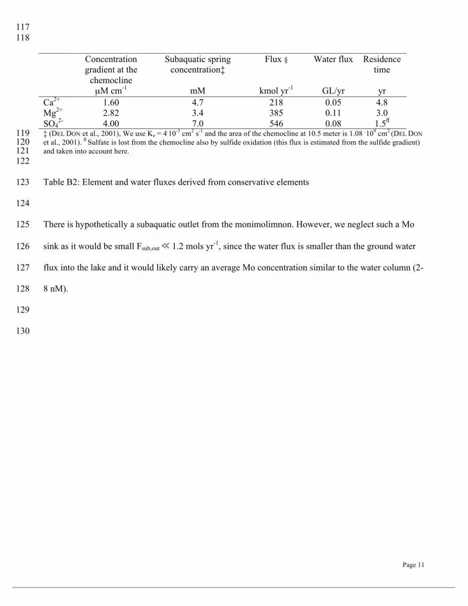
117 118

Concentration gradient at the

chemocline

Subaquatic spring concentration‡

Flux § Water flux Residence time

µM cm-1 mM kmol yr-1 GL/yr yr Ca2+ 1.60 4.7 218 0.05 4.8 Mg2+ 2.82 3.4 385 0.11 3.0 SO4

2- 4.00 7.0 546 0.08 1.5fl ‡ (DEL DON et al., 2001), We use Kz = 4.10-3 cm2 s-1 and the area of the chemocline at 10.5 meter is 1.08 .109 cm2 (DEL DON 119 et al., 2001). fl Sulfate is lost from the chemocline also by sulfide oxidation (this flux is estimated from the sulfide gradient) 120 and taken into account here. 121 122

Table B2: Element and water fluxes derived from conservative elements 123

124

There is hypothetically a subaquatic outlet from the monimolimnon. However, we neglect such a Mo 125

sink as it would be small Fsub,out 1.2 mols yr-1, since the water flux is smaller than the ground water 126

flux into the lake and it would likely carry an average Mo concentration similar to the water column (2-127

8 nM). 128

129

130

Page 12

130

Electronic Annex C: Reaction kinetics of molybdate conversion to thiomolybdate 131

132

The rate of sulfidation from molybdate to thiomolybdate species is driven by aqueous H2S through the 133

reaction MoO4-xSx2- + H2S ↔ MoO3-xSx+1

2- + H2O (where x = 0, 1, 2, 3 is the number of S atoms in the 134

reactant) (ERICKSON and HELZ, 2000). This reaction only occurs at low pH when dissociation of 135

hydrogen sulfides favor H2S (HERSHEY et al., 1988). Tetrathiomolybdate form only above a threshold 136

of H2S = 11 µM (ERICKSON and HELZ, 2000) and it would dominate in systems where there is enough 137

time for the reaction to proceed. However, the formation of tetrathiomolybdate by sulfidation occurs 138

over a longer time scale than the Mo residence time in the sulfidic zone of Lake Cadagno, so the 139

reaction would not have proceeded to its equilibrium state by the time of removal. 140

141

Sampling date measured ΣS2-

bottom water

pH calculated H2Saq

bottom water

June 8, 2006 237 7.11-7.02a 145-162

June 11, 2006 254 7.11-7.02a 155-173

June 15, 2006 261 7.11-7.02a 159-178

September 27, 2006 275 6.99-7.11 a 172-188

August 23, 2007 165.2 7.11 101

August 26, 2006 175.3 7.11 107

142

Table C 1: Measured ΣS2- and calculated concentrations of aqueous H2S. a Uncalibrated pH meter. 143

144

The time evolution of the Mo speciation in a sulfidic water body is described in Table 3 of ERICKSON 145

and HELZ, 2000: 146

Page 13

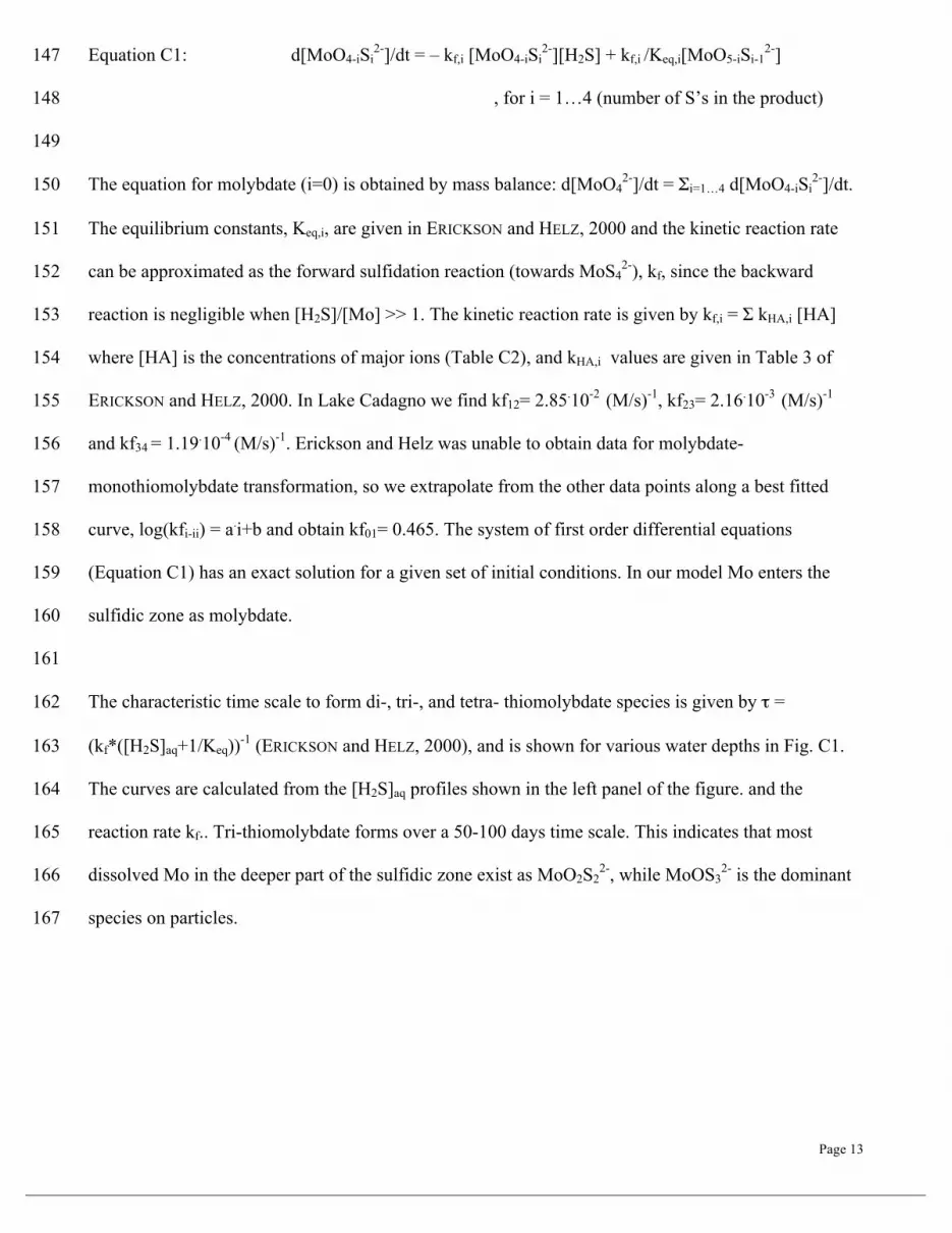
Equation C1: d[MoO4-iSi2-]/dt = – kf,i [MoO4-iSi

2-][H2S] + kf,i /Keq,i[MoO5-iSi-12-] 147

, for i = 1…4 (number of S’s in the product) 148

149

The equation for molybdate (i=0) is obtained by mass balance: d[MoO42-]/dt = Σi=1…4 d[MoO4-iSi

2-]/dt. 150

The equilibrium constants, Keq,i, are given in ERICKSON and HELZ, 2000 and the kinetic reaction rate 151

can be approximated as the forward sulfidation reaction (towards MoS42-), kf, since the backward 152

reaction is negligible when [H2S]/[Mo] >> 1. The kinetic reaction rate is given by kf,i = Σ kHA,i [HA] 153

where [HA] is the concentrations of major ions (Table C2), and kHA,i values are given in Table 3 of 154

ERICKSON and HELZ, 2000. In Lake Cadagno we find kf12= 2.85.10-2 (M/s)-1, kf23= 2.16.10-3 (M/s)-1 155

and kf34 = 1.19.10-4 (M/s)-1. Erickson and Helz was unable to obtain data for molybdate-156

monothiomolybdate transformation, so we extrapolate from the other data points along a best fitted 157

curve, log(kfi-ii) = a.i+b and obtain kf01= 0.465. The system of first order differential equations 158

(Equation C1) has an exact solution for a given set of initial conditions. In our model Mo enters the 159

sulfidic zone as molybdate. 160

161

The characteristic time scale to form di-, tri-, and tetra- thiomolybdate species is given by τ = 162

(kf*([H2S]aq+1/Keq))-1 (ERICKSON and HELZ, 2000), and is shown for various water depths in Fig. C1. 163

The curves are calculated from the [H2S]aq profiles shown in the left panel of the figure. and the 164

reaction rate kf.. Tri-thiomolybdate forms over a 50-100 days time scale. This indicates that most 165

dissolved Mo in the deeper part of the sulfidic zone exist as MoO2S22-, while MoOS3

2- is the dominant 166

species on particles. 167

Page 14

168

Figure C1: Left panel shows calculated H2S profiles for three field trips. The three right-most panels 169

show the characteristic time scale, τ, to form dithiomolybdate, trithiomolybdate, and 170

tetrathiomolybdate at various depth in Lake Cadagno, see text for details. 171

172

Species [HA] moles/liter NH4+ 2.50.10-5 H3O+ 7.94328.10-8 H2O 56 H2PO4- 2.30.10-6 HCO3- 1.58.10-6

Table C2: Ion concentrations in Lake Cadagno. 173 174

Modelling isotope fractionation in Lake Cadagno 175

We establish a mechanistic model of how Mo isotope fractionation is expressed in sulfidic basin when 176

Mo is scavenged by sinking particles in the form of oxythiomolybdate species. The model neglects the 177

mixing of water masses that can occur by advection and diffusion in the water column. All species are 178

in isotopic equilibrium allowing for equilibrium fractionation laws to apply. We fit the data to the 179

Cadagno water column, so that the sum of all species on particles and in the dissolved state give 180

observed total Mo profile: Σ(MoO4-xSx2-)particles + (MoO4-xSx

2-)dissolved = Mototal, and the cumulated 181

δ98Mo of all dissolved phases match observed isotope profile (using data from August 2007). However, 182

Page 15

the comparison must be made with caution since Lake Cadagno is also influenced by Mo supply from 183

ground water and Mo release from sediments. Therefore, the goal is not to optimally fit the data, but 184

instead show common features between model and observation. 185

186

Isotope fractionation results from the constant isotopic offset between Mo species. The isotope 187

fractionation factors have been derived from quantum mechanical theory (TOSSELL, 2005) and the 188

values used here,are temperature corrected isotope fractionation factors Δ01 = -1.4‰, Δ12 = -1.4‰, Δ23 189

= -1.7‰, Δ34 = -1.7‰ (interpolation of results in Tossell, 2005). Again, the first and second indices 190

represent the number of S atoms in the reactant and product, respectively. The isotopic composition of 191

one species can be calculated from the neighboring species, e.g. δ98Motetra = δ98Motri + Δ34 or generally: 192

δ98Moj = δ98Moi + Δij 193

194

The time evolution of the Mo species distribution and their isotopic composition is shown in Fig. C2. 195

The Mo residence time in Lake Cadagno is 80-130 days, and consequently MoO3S2- must be the 196

dominant Mo species in the deeper part of the lake. MoO2S22- and MoS4

2 would be second most 197

abundant species at slightly earlier and later times, respectively. 198

199

We allow particles and waters to contain a mixture of oxythiomolybdate species. The particle affinity 200

of each species depends on the nature of scavenging particles, and controlled experiments with particle 201

complexation with organic matter have not yet been published. However, adsorption experiments with 202

FeS (HELZ et al., 2004) suggest that the more sulfidized MoO4-xSx2- anions are more susceptible to 203

scavenging. Particles in the oxic zone where only MoO42- is abundant, do not accumulate Mo, so the 204

particle affinities defined as Ki = [MoO4-iSi2-]particulate/[MoO4-iSi

2-]dissolved (particle-associated Mo relative 205

to dissolved Mo per unit volume) follows: K0 = 0 ≤ K1 ≤ K2 < K3 < K4. At a given H2S level, the 206

resulting fractionation on particles relative to dissolved Mo, Δ98MoPD, depends on time available for 207

reaction and the actual choice of Ki. These relationships are explored in Fig. C3 and the Fig. C4, 208

respectively. We compare the outcome of the model to available data for natural sulfidic systems. A 209

compilation of observed net isotope fractionations and estimates of the time available for reaction in 210

the system is shown in Table 8. The observational results are plotted as error bars in Fig. C4 and Fig. 211

11. 212

213

Page 16

214 Figure C2: Model prediction of concentration and isotopic composition for each oxythimolydate 215

species in Lake Cadagno if the time available for reaction is a) 50 days, b) 500 days, and c) infinite 216

time (equilibrium state). 217

Page 17

218 Figure C3: Model prediction of the concentration (left side) and δ98Mo profiles (right side) for 219

dissolved and particulate Mo, when particle affinities are chosen to be: K0 = K1 = 0, K2 = 1, K3 = 25, 220

K4 = 100. Panels a-c) shows the distribution at three different times: a) after 50 days, b) 500 days, and 221

c) at equilibrium, t = ∞.222

Page 18

223

224 Figure C.4: Model predictions of isotope fractionation as a function of H2S. In all panels three curves 225

are plotted to represent the time available for reaction in Cadagno (black), Black Sea (blue) and 226

Cariaco Basin (cyan). In each panel a)-d), the net isotope fractionation expressed in the sediment, 227

Δ98MoSS, is shown above the predicted isotope fractionation on sinking particles relative to residual 228

sulfidic water, Δ98MoPD. Observed data is plotted with error bars of the respective grey scale. Particle 229

affinities K = (K0, K1, K2, K3, K4) varies between the panels: a) K = (0, 1, 2, 3, 4), b) K = (0, 0, 1, 3, 4), 230

c) K = (0, 1, 1, 25, 100), and d) K = (0, 0, 1, 10, 100). Our favorite model K = (0, 0, 1, 25, 100) is 231

shown in Fig. 11. 232

233

All particulate Mo is retained at the depth where these form and do not take into account that particles 234

sink to the sediment. Thus, the modeled particulate Mo profile exceeds the observed profile of Mo on 235

suspended particles, and one cannot compare observations and model directly. Instead, we emphasize 236

Page 19

that this model can explain how the observed Δ98MoPD is about -1‰ in the deep part of the lake, while 237

some Mo still remains in solution (Fig. C3, a). 238

239

The model depends strongly on oxythiomolybdate particle affinities, and we here explore the possible 240

solutions. A linear increasing particle affinity, K = (0, 1, 2, 3, 4), cause too little net fractionation at 241

low H2S and no isotopic offset between Mo on sinking particles and residual dissolved Mo in the 242

sulfidic waters (Fig. C4 a). The low end H2S can be explained by monothiomolybdate being non-243

particle reactive, K = (0, 0, 1, 3, 4), panel b. In order to accommodate the δ98/95Mo offset between 244

sinking particles and sulfidic waters observed in Lake Cadagno, the particle affinity of trithiomolybdate 245

must be dramatically higher than less sulfidated species, K = (0, 1, 1, 10, 100), panel c). A combination 246

of low particle affinity for monothiomolybdate and very high particle affinities for tri- and 247

tetrathiomolybdate allows for a reasonable fit both at the low and high end of H2S values. Yet, the 248

model predicts too high net isotope fractionation for the 10-50 µM range. Further studies in such 249

settings are needed to understand both temporal variations of bottom water [H2S] and Mo removal. 250

Controlled laboratory experiments should challenge if the particle affinity of trithiomolybdate is 251

dramatically higher than less sulfidated species and if the proposed style of ion-particle interaction can 252

be justified. 253

254

Page 20

254

References to electronic annex: 255

Del Don, C., Hanselmann, K. W., Peduzzi, R., and Bachofen, R., 2001. The meromictic alpine Lake 256 Cadagno: Orographical and biogeochemical description. Aquatic Sciences 63, 70-90. 257

Erickson, B. E. and Helz, G. R., 2000. Molybdenum(VI) speciation in sulfidic waters: Stability and 258 lability of thiomolybdates. Geochimica Et Cosmochimica Acta 64, 1149-1158.. 259

Helz, G. R., Vorlicek, T. P., and Kahn, M. D., 2004. Molybdenum scavenging by iron monosulfide. 260 Environmental Science & Technology 38, 4263-4268. 261

Hershey, J. P., Plese, T., and Millero, F. J., 1988. The PK1-* for the Dissociation of H2S in Various 262 Ionic Media. Geochimica Et Cosmochimica Acta 52, 2047-2051. 263

Imboden, D. M., Wüest, A., 1995. Mixing Mechanisms in Lakes. Springer Verlag. , Heidelberg. 264 Tossell, J. A., 2005. Calculating the partitioning of the isotopes of Mo between oxidic and sulfidic 265

species in aqueous solution. Geochimica Et Cosmochimica Acta 69, 2981-2993. 266 267 268

269