Document de travail 2013-05

“Tax evasion, tax corruption and stochastic growth”

Fred CELIMENE, Gilles DUFRENOT, Gisèle MOPHOU & Gaston N’GUEREKATA

Février 2013

Centre d’Etude et de Recherche en Economie, Gestion, Modélisation et Informatique Appliquée

Université des Antilles et de la Guyane. Faculté de Droit et d’Economie de la Martinique. Campus de Schoelcher - Martinique FWIB.P. 7209 - 97275 Schoelcher Cedex - Tél. : 0596. 72.74.00 - Fax. : 0596. 72.74.03

www.ceregmia.eu

Tax evasion, tax corruption and stochasticgrowth

Fred Célimène� Gilles Dufrénoty Gisèle Mophouz

Gaston N�Guérékatax

February 20th, 2013

Abstract

This paper presents a continuous time stochastic growth model tostudy the e¤ects of tax evasion and tax corruption on the level and volatil-ity of private investment and public spending. Our results suggest thatthere do exist several regimes of mean growth and growth volatility, de-pending upon the consumer�s degree of risk aversion, the tax income yield,the risk-adjusted return of the agent�s portfolio, the productivity of publicspending. We �nd that public spending is described asymptotically by anincomplete upper Gamma distribution, while private capital is describedby a power law distribution. Depending upon the values of the parame-ters of these distributions, growth can be characterized by extreme values(high volatility) when the return to taxation lies under a certain thresholdand/or when the risk-adjusted return of investing the proceeds of illegalactivities evolves above a given threshold. We provide an empirical illus-tration of the model.

Key words : Stochastic growth; tax evasion; tax corruption

JEL Classi�cation : H26;D91;O41

�Université des Antilles et de la Guyane, Laboratoire CEREGMIA. Université des An-tilles et de La Guyane, Campus Schoelcher, B.P. 7209, 97275 Schoelcher Cédex(FWI). Email:fred.celimene@martinique.univ-ag.fr

yAix-Marseille Université (Aix-Marseille School of Economics &CNRS&EHESS), Banquede France and CEPII, Château Lafarge, route des Milles, 13290, Aix-en-Provence Les Milles.Email: gilles.dufrenot@univ-amu.fr

zUniversité des Antilles et de la Guyane, Laboratoire CEREGMIA. Université desAntilles et de La Guyane, Campus Fouillole 97159 Pointe-à-Pitre Guadeloupe (FWI).Email:gmophou@univ-ag.fr

xMorgan State University, Baltimore, MD, USA

1

1 Introduction

This paper tries to shed some light on the impact of tax evasion and tax cor-ruption on private investment and government spending, two key determinantsof the growth rate and volatility of per-capita GDP. In poor countries, in whichthe public sector is an essential contributor to the economic growth, stagnationand severe swings in economic growth are related to the de�cient tax collectionsystems which do not allow to provide the minimum amount of public goodsand services necessary for productive activities like infrastructure, education, orinvestment (see Friedman et al., 2000). Following the recommendation of themultilateral and bilateral donors, as well as of the international organizations,governments are willing to reduce corruption and tax evasion to avoid loss oftax revenues. But many developing countries still appear to be stuck in a vi-cious circle of both tax corruption and tax evasion, a phenomenon to which thetheoretical and empirical literature have paid a great attention (see, among oth-ers, Mauro, 2004). Fighting corruption may be di¢ cult because of rent-seekingactivities and building a technology that detects tax evaders is expensive. Asfar as we question the implication for growth and its volatility, a commonlyaccepted answer consists in saying that countries in such a situation are likelyto achieve a bad macroeconomic equilibrium, namely the coexistence of a lowgrowth rate and a high volatility of per-capita GDP. Indeed, according to theliterature, corruption is an important factor contributing to growth volatility(see Denizer et al., 2000).In this paper, we maintain that in such situations in which a government is

unable to reduce the level of corruption and tax evasion, an alternative solutionis either to allow the resources of the evaded tax to be invested in equities (by al-lowing a private equity market to �ourish, private capital becomes a substitutefor public spending in the production function), or to raise the productivityof public spending to attenuate the negative externalities of tax evasion onproductive public expenditure. To develop these ideas, we use a standard port-folio argument by adopting an open economy stochastic growth model, in linewith previous models like Turnovsky (1993), Grinols and Turnovsky (1993),Turnovsky (1999). Public goods and private investment are both productiveinputs in the production function.An important di¤erence with the previous literature is that the risk that

interact with growth is not exogenous, but stems from endogenous sources: tax corruption and tax evasion. Speci�cally, the uncertainty in the modelcomes from the fact that hiding income from the tax administration and o¤er-ing briberies to inspectors are risky activities. Cheating is an uncertain activitybecause there is a probability of being detected and a probability to be con-fronted to a corrupted inspector. People may decide to shelter themselves froma tax payment, but at the cost of paying bribes to civil servants. Our resultssuggest that there do exist several regimes of mean growth and growth volatility,depending upon the consumer�s degree of risk aversion, the tax income yield, therisk-adjusted return of the agent�s portfolio, the productivity of public spend-ing. Importantly, the model considers tax evasion, private capital and public

2

spending as endogenous variables and creates a loop between them.We build upon the idea that tax evasion and tax corruption are non-separable

when tax collection is performed by corruptible inspectors (see Hindricks et al.,1999, Sanyal et al., 2000). However, our model di¤ers from previous models onthe same topic in several respects. Lin and Yang (2001) also consider a stochas-tic growth model of tax evasion, but with no speci�c role for corruption and norole for public spending as an input in the production function. Chen (2003)also considers a model of tax evasion with productive public capital. Unlike theauthor, we do not consider any optimizing behavior from the government side.Further, in our model tax evasion generates uncertainty and thus a randomnesson production. Dzhumashev (2007) uses a framework like ours, but his modelapplies to a closed economy. In our case, opening the economy allows intro-ducing wealth e¤ects in the model. Further, by considering a general CRRAutility function, we show that the impact on capital accumulation of tax cor-ruption and tax evasion depends upon a trade-o¤ between the risk aversion andthe saving behavior. Finally, Cerquetti and Coppier (2011) address the issueof the e¤ects of tax evasion and tax corruption on economic growth and theyapply a game-theoretical approach to a Ramsey model. The authors focus onthe strategic behaviors of consumers and bureaucrats and this issue is put ofthe scope of this paper.We obtain closed-form solutions for the steady state invariant distributions.

We �nd that public spending is described asymptotically by an incomplete upperGamma distribution, while private capital is described by a power law distrib-ution. These distributions have parameters described by the return to taxationand the portfolio performance of the evasion and corruption activity. The inter-esting point is that growth can be characterized by extreme values (high volatil-ity) when the return to taxation lies under a certain threshold and/or when therisk-adjusted return of investing the proceeds of illegal activities evolves abovea given threshold.The remainder of the paper is organized as follows. Section 2 sets out the

model. In Section 3, we study the optimal choice of the domestic agent. Section4 presents the steady state distributions, while Section 5 contains the resultsof a comparative dynamics analysis. Section 6 summarizes the main resultsfrom the formal model and Section 7 presents an empirical illustration on theSouthern African countries. Finally Section 8 concludes.

2 The model

This section presents a continuous time stochastic growth model. We describea representative agent�choice and present the dynamics of saving and publicspending in a stochastic environment. The source of uncertainty is not thetechnology but tax evasion and tax corruption. Tax People whi are fraudingcan be caught, but they may face corruptible bureaucrats to whom they proposebribes. Tax corruption thus occurs through bribery to avoid paying the penaltyfor tax evasion. Tax evasion and tax corruption are risky activities. We assume

3

that perceived and objective probabilities of getting caught and of paying bribesare the same and that the detection technology used by the bureaucrats iscostless.

2.1 Tax fraud and tax corruption as a source of randomincome

2.1.1 Production

We consider an open economy called the domestic country and the rest of theworld referred as the foreign country. In each country we consider a societypopulated with a continuum of individuals with measure 1. An individual livesforever (we have in�nitely lived representative agents). She supplies her laborforce inelastically to the productive sector. for purpose of simplicity we noram-lize the labor supply to 1. In addition to consumers and �rms, politicians livein both the domestic and foreign economies. They provide a productive inputin public spending �nanced out of tax revenue.Private �rms in the domestic economy produce a consumption good with

the following production technology:

c(t) = y(t) = A(t)k(t), A(t) = � [g(t)]1=�

;(k(t); g(t)) 2 [0;+1)� [0;+1); (1)

where c(t), y(t) are per-capita consumption and output, k(t) andA(t) are respec-tively the (private) capital-labor ratio and productivity. The latter is assumedto depend upon public goods and services (roads, public health, education, etc)provided by the bureaucrats or politicians and we assume decreasing returns ofthe technology for public goods (� > 1). The price of the consumption good isnormalized to 1. g(t) is per-capita public spending. Similarly, the productiontechnology in the foreign country is given by

c�(t) = y�(t) = A�(t)k�(t), A�(t) = �� [g�(t)]1=��

;(k�(t); g�(t)) 2 [0;+1)� [0;+1); (2)

For simplicity, we assume that private capital does not depreciate. g is a purepublic good (government goods and services are neither rival nor excludable).

2.1.2 Tax evasion and tax corruption

Our modelling of tax evasion relies upon Allingham and Sandmo (1972) andYitzhaki (1974). Taxes are used to �nance public goods and services. We donot make explicit the production function of the public good since this is notimportant here.An agent chooses to hide a fraction e(t) of her income from the government

and we assume that 0 < e(t) < 1. Yet, politicians try to detect tax evasion. Theprobability of being detected is p (0 < p < 1). A consumer who is detected isasked to pay the legal tax �e(t)y(t) plus a penalty de�ned as a fraction s of the

4

undeclared income, s�e(t)y(t).� is the legal tax rate (0 < � < 1) and we havea similar de�nition for the legal tax rate in the foreign country (0 < �� < 1).To avoid paying the penalty, the detected evader can pay a bribe to inspectors.The latter are corruptible with a probability p1 (0 < p1 < 1). Denoting � thepenalty rate when there are no bribes, we assume that the detected evader canpay back less than � and we denote b the penalty rate when politicians arecorrupted (b < �).The penalty rate is thus a random variable

�1 =

��; w:p: 1� p1b; w:p: p1

���� ; (3)

and the expected value of the penalty rate is E [�1] = � = p1b + (1 � p1)�.Therefore, the random return of a unit of evaded tax is

x1 =

�1� �; w:p: p1; w:p: 1� p

���� : (4)

The expected return on a unit of evaded tax is thus E [x1] = x1 = 1 � �p.Tax evasion is worth if x1 > 0, which implies �p < 1. x1 is a binomial process ora Poisson process if p ! 0. Assuming that the domestic economy is composedof an in�nite number of consumer who behave in a similar way, both processestends to a Normal law. Therefore x1 converges to a Normal law with mean x1and a variance �21 = p(1� p)�2.The dynamics of the random gain induced by tax evasion is described by the

following stochastic di¤erential equation (SDE):

dx1(t) = x1�e(t)y(t)dt+ �1�e(t)y(t)dz1(t); (5)

where z1(t) is a Brownian motion process.Similarly, in the foreign country we have

dx�1(t) = x�1��e�(t)y�(t)dt+ ��1�

�e�(t)y�(t)dz�1(t); (6)

where z�1(t) is a Brownian motion process

2.1.3 Portfolio diversi�cation and the dynamics of wealth

A household spends a fraction of his income in consumption and uses the re-maining income to buy equities whose values represent a share of the physicalcapital of the domestic country and of the foreign country. We assume that thepopulation size is the same in both countries. We de�ne

k(t) = kd(t) + kf (t) and k�(t) = k�d(t) + k�f (t); (7)

wherekd(t) is the domestic per-capita capital owned by the domestic agent,kf (t) is the domestic per-capita capital owned by the foreign agent,

5

k�d(t) is the foreign per-capita capital owned by the domestic agent,k�f (t) is the foreign per-capita capital owned by the foreign agent.Denoting w(t) the average wealth of the domestic agent (per-capita wealth

or saving), nd(t) and n�d(t) the shares of domestic and foreign capital in the thedomestic agent�total wealth, we have

nd(t) =kd(t)

w(t); n�d(t) =

k�d(t)

w(t), w(t) = kd(t) + k

�d(t): (8)

We have similar relationships for the foreign consumer:

n�f (t) =k�f (t)

w�(t); nf (t) =

kf (t)

w�(t), w�(t) = kf (t) + k

�f (t): (9)

where w�(t) is per-capita wealth in the foreign country. We assume perfect cap-ital mobility without restrictions on asset trade. We further assume that thereis a demand for portfolio diversi�cation. This implies that nd(t), n�d(t); n

�f (t)

and nf (t) are strictly positive and less than 1.Wealth (or saving) is a random variable because the expected return on

tax evasion is a random variable. Each unit of income hidden yields x1 onaverage with more or less �1. Assuming that per-capita consumption evolves ata deterministic rate c(t)dt, we have

dw(t) = f[1� � + x1�e(t)]A(t)kd(t) + [1� �� + x�1��e�(t)]A�(t)k�d(t)(10)�c(t)gdt+ �1�e(t)A(t)kd(t)dz1(t) + ��1��e�(t)k�d(t)dz�1(t);

from which we deduce the rate of accumulation of assets by the domestic agent:

dw(t)

w(t)= (t)dt+ !1(t)dz1(t) + !

�1(t)dz

�1(t); (11)

where

(t) = R(t)nd(t) +R�(t)(1� nd(t))�

c(t)

w(t); (12)

R(t) = (1� � + x1�e(t))A(t);R�(t) = (1� �� + x�1��e�(t))A�(t):

and

!1(t) = �1�e(t)A(t);

!�1(t) = ��1��e�(t)A�(t);

R(t) and R�(t) are the gross rates of returns of one unit of capital investedrespectively in the domestic and in the foreign countries. They depend uponthe tax rates, the expected returns of a unit of evaded tax and the proportionsof revenues hidden. !1(t) and !�1(t) are the risk of one unit of capital investedin the home and foreign countries. Therefore R(t)nd(t)+R�(t)(1�nd(t)) is the

6

gross rate of return of the domestic agent�s portfolio. For the foreign agent, wehave similar relationships.We assume that the following inequalities hold simultaneously R(t) > R�(t)

and !1(t) > !�1(t) or R(t) < R�(t) and !1(t) < !�1(t) (this is a standardassumption in any portfolio model with risky assets). This implies that weeither have x1 > x�1 and �1 > ��1, or x1 < x�1 and �1 < ��1. In the �rstcase, the expected return from tax evasion and tax corruption is higher butmore risky in the home country than in the foreign country. This happens forinstance when the probability of being caught in the domestic country is lowerin comparison with the same probability in the foreign country (p < p�), butif, upon catching an evader, the government imposes a higher penalty (� >

��) because the politicians are less corruptible (p1 < p�1). However, this same

situation could also arise with a higher probability of being detected (p > p�)because controls are more frequent), but if, upon being detected, the penaltyrate is lower because politicians are more corruptible (� < �

�and p1 > p�1).

2.2 The utility function

The consumer�s preferences are represented by an isoelastic utility function.We assume that she obtains utility from private consumption. The objectivefunction is

U = E0

Z 1

0

(1= ) (c(t)) e��tdt: (13)

We assume that �1 < < 0; � > 0. � is the time preference rate. 1 � is the Arrow-Pratt coe¢ cient of relative risk aversion. E0 is the expectationat time t = 0. Unlike other models developed in the stochastic growth liter-ature, we assume that public spending do not enhance the marginal utility ofconsumption, but only the productivity of private capital. This is a major dif-ference with, for example, Turnovsky (1999). The reason is that the situationwe consider applies to poor countries, which have no social insurance systems,where the quality of institutions and governance are too weak to allow the pro-vision of sound public service to people (for instance, public order and safetyor the provision of medical services), and where political leader are not alwaysaccountable for their actions. Therefore, we do not address issues such as �nd-ing the optimal size of the public sector, or studying the provision of publicspending that maximizes the welfare.

2.3 The dynamics of public spending

Public goods and services are �nanced out of tax income. The random returnto income taxation is

�(t) =

��1(t) = �(1 + se(t))A(t)k(t); w:p: p�2(t) = �(1� e(t))A(t)k(t); w:p: 1� p (14)

Tax revenue is a random variable and so is per-capita public spending. As-suming a zero �scal balance, the stochastic process describing the dynamics of

7

public spending is therefore

dg(t) = �1(t)g(t)1=�dt+ �2(t)g(t)

2=�dZg(t); (15)

where Zg(t) is a Brownian motion process and

�1(t) = p�1(t) + (1� p)�2(t)= �k(t) fp�(1 + se(t)) + (1� p)�(1� e(t))g ; (16)

and

�2(t) = p(1� p)�2k(t)2��2(1 + se(t))2 + �2(1� e(t))2

(17)

�2�2(1 + se(t))(1� e(t)): (18)

(15) is a nonlinear SDE with drift and di¤usion components which bothdepend on tax evasion behavior and tax corruption.

3 The optimal choice of the domestic agent

An agent faces the following intertemporal utility maximization problem. Shemaximizes (13) subject to the constraint (11) with w(0) = w0.

Proposition 1 The optimal choice of a consumer in the domestic country isgiven by the following unique interior solution (see the proof in Appendix 1)8>>>>>>>>>>>><>>>>>>>>>>>>:

(1� ) ec(t)w(t) = � � 2 [1� ]

�(!1(t))

2 + (!�1(t))2�~n2d

+ 2 [1� ] (!

�1(t))

2

� R�(t);

~nd(t) =(1� �)A(t)�R�(t)[1� ] (!�1(t))2

+ 1;

~e(t) =A(t) �x1�

[1� ] [�1�A(t)]2 ~nd(t):

(19)

The �rst equation is obtained from the equality between the marginal utilityof consumption and the marginal utility of wealth, which leads:

~c(t) = fV 0(w(t))g1

�1 (20)

where V is the value function.The second equation is an arbitrage equation obtained from the �rst-order

condition of the objective function obtained using the Jacobi-Hamilton-Bellmanequation with respect to nd(t). This yields

R(t)�AP (w)!1(t)2nd(t) = R�(t)�AP (w)!�1(t)2n�d(t); (21)

8

where AP (w) is the absolute value of the Arrow-Pratt relative risk aversioncoe¢ cient assumed to be constant:

AP (w) =wV

00(w)

V 0(w): (22)

Equation (21) says that the risk-adjusted gross returns of one unit of capitalinvested in the domestic and foreign countries are equalized. The risk can bedecomposed into several components. Its depends upon the share of capitalinvested out of total wealth in the domestic and foreign countries, upon theuncertainty from tax evasion and corruption and upon the agent�s behaviortowards risk. The risk premium is therefore a function of the degree of relativerisk aversion and of the di¤erence in the uncertainty of fraud and corruptingbureaucrats in both countries:

R(t)�R�(t) = AP (w)�!1(t)

2nd(t)� !�1(t)n�d(t)2�

(23)

The third equation is obtained by equalizing to zero the derivative of theobjective function with respect to e(t). This yields

~e(t) =

�1

�AP (w)

��x1�21

��1

�

��1

yd(t)=w(t)

�: (24)

The optimal decision of tax fraud varies positively with the risk-adjustedreturn of fraud and with the degree of risk aversion, negatively with the taxrate and the domestic revenue as share of the agent�s wealth. A system inwhich the tax rate is high is an incentive to cheat. Conversely, the motivationfor a tax fraud diminishes as domestic production represents a high proportionof an individual�s total wealth.The optimization problem facing the foreign agent is similar, but is not

studied here since our focus is on the domestic country.The household�s optimal solution does not lead to a closed-form solution, but

all the variables are determined simultaneously. The solution is well de�ned ifthe three variables lie in the unit interval (0; 1). This requires some assumptionsto guarantee that this holds.Firstly, using the expression of nd(t) in Appendix 1, the condition 0 <end(t) < 1 is equivalent to imposing a lower and upper bound on R�(t):

(1� �)A(t) < R�(t) < (1� �)A(t) + (1� )!�1(t)2: (25)

One can interpret nd(t) as the domestic �nancial market depth, and also asthe degree of �nancial openness. A value near 1 indicates that there are strongrestrictions on the international mobility of capital assets, while a value near 0re�ect a situation of perfect mobility and perfect substitution between domesticand foreign assets. We exclude the situation of preferred habitat where savingwould be entirely invested in either domestic or foreign capital. The aboveinequality indicates that this is the case if investing abroad yields a minimumgross rate of return on each unit of foreign capital owned (the lower bound). To

9

avoid a situation of a complete depletion of domestic capital (capital out�owsthat would lead to end(t) = 0), the foreign gross rate of return must be boundedabove (the upper bound). From (19), it is seen that whenever end(t) > 0, thisinequality also holds for ~e(t) and ec(t)

w(t) .From (19), ~e(t) < 1 if the expected return on one unit of evaded tax, adjusted

by the risk of tax evasion and tax corruption, is bounded above (the gain fromcheating is limited). Formally, ~e(t) < 1 implies the following inequality:

x1�21

< �A(t)(1� )end(t): (26)

Finally, the agent does not spend her whole wealth in consumption spendingif the marginal utility of wealth is bounded above. Indeed, in Appendix 1 weshow that ec(t)

w(t)= [V 0(!)]

1= �1: (27)

Therefore ec(t)w(t)

< 1; if V 0(!) < !(t) �1: (28)

4 Steady state distributions

4.1 De�nition of the equilibrium

For a given sequence ofnA�(t); e�(t); en�f (t); ec�(t)w�(t) ; y

�(t); k�(t)o10and initial val-

ues ~e(0), ec(0)w(0) , end(0), g(0), y(0), k(0);the equilibrium is a sequence�

A(t); e(t); end(t); ec(t)w(t)

; y(t); k(t)

�10

;

where each variable is de�ned by a distribution, that satis�es the followingconditions:

i) these variables satisfy the agent�s optimal choice,ii) domestic capital growths at the same rate as saving,iii) the government�s budget constraint is described by the SDE (15),iv) the economy�s capital and �nancial account is balanced.v) the constraints (25), (26) and (28) apply.

Condition (i) implies that the equilibrium path must satisfy the system (19).As shown in Appendix 1, the convexity of the maximization problem impliesthe unicity of the optimal solution.

Condition (ii) implies that the dynamics of capital obeys the following SDE:

dk(t) =dw(t)

w(t)k(t) = (t)k(t)dt+1(t)k(t)dZk(t); (29)

10

where we have substituted a new di¤usion component 1(t)dZk(t) for the twolocal martingale terms !1(t)dz1(t) and !�1(t)dz

�1(t) in Equation (11). The solu-

tion of this SDE can be written as

d ln k(t) =

� (t)� 1

221(t)

�dt+1(t)dZk(t); (30)

which implies

k(t) = k(0) exp

�Z t

0

( (s)� 12(1(s))

2)ds

�: (31)

Condition (iii) implies that the dynamics of A(t) can be found by applyingthe Ito lemma. We have

A(t) = � [g(t)]1=� and dg(t) = e�1(t)dt+ e�2(t)dzg(t); (32)

where e�1(t) = �1(t) [g(t)]1=� and e�2(t) = �2(t) [g(t)]

2=� with �1(t) and �2(t)de�ned by (16) and (17). Applying the Ito lemma, we have

dA(t) =

�e�1(t)@A(t)@g(t)

+1

2(e�2(t))2 @2A(t)

@g(t)2

�dt+ (33)

e�2(t)@A(t)@g(t)

dzg(t);

ordA(t) = �(t)A(t)dt+ �(t)A(t)dzg(t); (34)

where

�(t) = e�1(t)(�=g(t)) + (1� ��)(�=g(t)2)e�2(t)2; (35)

�(t) = (�=g(t))e�2(t): (36)

Equation (34) implies

A(t) = A(0) exp

�Z t

0

(�(s)� 12(�(s))2)ds

�: (37)

(31) and (37) are not closed-form solutions of (??) and (34) because k(t)and A(t) also appear in (t), 1(t), �(t) and �(t) and in (19). k(t) and A(t)are the two important state variables in the model, since they determine thedynamics of all the other variables. The equilibrium is described by a randomsequence of the variables or by a distribution. Indeed, as is seen from ourequations, the dynamics is the results of a deterministic drift component andof a di¤usion component where the variance of the variables is used to de�netheir distribution. The stochastic nature of the model entirely comesfrom theuncertain income caused by tax evasion and tax corruption.

11

4.2 Su¢ cient conditions for the existence of a long-runstochastic steady state

We focus on the dynamics of the variables of our model in the neighborhood ofthe long-run stochastic steady state. Such a state is characterized, in systems ofSDE, by a steady stable distribution. We study the conditions for the existenceof such a distribution for per-capita GDP. Since the latter depends upon k(t)and A(t), we check the validity of some conditions for these variables to have alimit stable distribution. We shall prove the following two propositions:

Proposition 2 k(t) has two bounds 0 and 1. The zero bound is inaccessi-ble if s=(s1)

2 is above a threshold value (here 1=2) and the in�nite bound isinaccessible if s=(s1)

2 is below a threshold value (1=2).

Proposition 3 A(t) has two bounds 0 and 1. The zero bound is inaccessi-ble if �s=(�s)2 is above a threshold value (here 1=2) and the in�nite bound isinaccessible if �s=(�s)2 is below a threshold value (1=2).

Before proving these propositions, we brie�y explain what they mean. Anexponent s on a variable indicates that the variable is considered in the neigh-borhood of the random steady state. It is noteworthy that production is possiblewith private capital and public spending. But since the latter is �nanced outof tax income, if private capital is nil, then the production becomes nil andthere are neither tax revenues, nor spending. The quantity s=(s1)

2 can beinterpreted as a Sharpe ratio indicating the performance of the agent�s portfo-lio that consists of domestic and foreign equities (private domestic and foreigncapital). The �rst proposition says that, when the performance of the portfoliois high enough, there is an incentive for cheating and thus the economy neverconverges to a situation in which the household decides to consume her wholewealth without investing in private capital. On the other side, when income ishidden and invested into productive capital, this increases the amount of taxincome available for the �nancing of public goods and services increases, whichraises production and in turn the return to cheating. To avoid a situation inwhich the agent would decide to reduce her consumption to zero while invest-ing all her wealth in private capital, the performance of the portfolio must bebounded above. It is important to notice that, for given value of p; p1; b; �; s, wehave either s=(s1)

2 < 1=2 or s=(s1)2 > 1=2. Therefore, if we would consider

per-capita capital alone, we could not avoid either a depletion or an explosion ofthe economy. We therefore need other conditions on public spending, given inthe second proposition. The ratio �s=(�s)2 can be viewed as a proxy of the risk-adjusted random income to taxation weighted by the marginal productivity ofpublic spending (see Equation (19)). For the economy not to extinct (A(t) = 0),we need a minimum tax income yield (�s > 2(�s)2). But tax income should bebounded above to avoid an in�nite accumulation of public spending that wouldyield an in�nite per-capita output (�s < 2(�s)2). Again, if we would considerper-capita spending alone, we could not avoid either a depletion or an explosionof the economy. This yields four cases (see Table 1)

12

INSERT TABLE 1 ABOUT HERE

If both A and k equal zero or in�nity, then there is no random steady statein the economy. Therefore, the set of parameters p; p1; b; �; s must be de�ned insuch a way that we either have the conditions s=(s1)

2 < 1=2 and �s=(�s)2 >1=2, or s=(s1)

2 > 1=2 and �s=(�s)2 < 1=2. Since, in the neighborhood of therandom steady state, both variables are attracted towards opposite directions,the conditions imply that there is an equilibrium value for per-capita output.The two polar cases �gure out two types of economies. On the one hand, if taxcollection systems are e¢ cient and government manage to �ght corruption, taxevasion becomes unattractive and there is a low level of private capital due to lowconcealed income. But in turn, the economy will be �nanced by a high amount ofpublic spending. On the other side, cheating and o¤ering bribes to bureaucratsmay be easy, thereby implying high opportunities to invest the earned income inprivate equities. In this case per-capita income will be �nanced by private capitalat the expense of public spending. In our model, public and private capital arethus substitutable. One implication is that tax evasion and tax corruption arenot necessarily harmful for growth, provided that there exist equity markets inwhich the proceeds of concealed income can be invested. If people have a lowpropensity to consume their wealth, but instead a high propensity to save, taxevasion can be viewed as similar to tax exemption. This is exactly the way theso-called "tax havens" function. We now prove the propositions.

Proof. We use the following lemma that apply to SDE (see Karlin and Taylor(1981)).Lemma. Consider a di¤usion process X(t) = a(t)dt + b(t)ZX(t) where

ZX(t) is a Brownian motion process. Assume that this process has two boundsr1 and r2. Su¢ cient conditions: the two bounds are inaccessible, if8x0 2 [r1; r2] ; S(r1) = �1; S(r2) = +1; where

S(x) =

Z x

x(0)

s(u)du, s(x) = exp

(�2Z x

x(0)

a(u)

b2(u)du

): (38)

s(x) and S(x) are called respectively the scale density function and the scalefunction. In our case, we have

s(k) = [k=k(0)]�2 s=(s1)

2

;

S(k) =k(0)2

s=(s1)2

(s1)2

�2 s + (s1)2k�2 s+(s1)

2

(s1)2 � s1

�2 s + (s1)2k(0),

and

limk!0

S(k) = �1; if 2 s � (s1)2 > 0;

limk!1

S(k) = +1; if 2 s � (s1)2 < 0:

The proof is similar for A(t).

13

4.3 Steady state distribution for g(t)

We prove and comment the following proposition:

Proposition 4 A closed-form expression of the invariant steady-state distri-bution for public spending is given by the following upper incomplete Gammadistribution:

P (g) = Ks1K

s3

�(�;Ks2g

��3� )

�(�); � 2 (1; 3); � =

4� �3� � ; (39)

where Ks1 , K

s2 and K

s3are constants:

Ks1 =

1

(�s2)2exp

nKs2g(0)

(��3)=�o;Ks

2 =2�s1(�s2)

2 ��

3� � ; (40)

Ks3 =

�1

Ks2

�(�4+�)=(��3)�

� � 3 : (41)

�s1 and �s2 are (16) and (17) de�ned in the neighborhood of the random steady

state and

�(�) =

Z 1

0

g��1 exp(�g)dg and �(�; y) =

Z 1

y

g��1 exp(�g)dg; � > 0; x > 0:

The proof of this proposition is in Appendix 2. Let us comment some ofits implications. In our stochastic growth model, the growth rate of per-capitaGDP is in�uenced by the volatility a¤ecting per-capita GDP, or similarly bythe volatility a¤ecting at least one of its components, namely capital or publicspending. The main characteristics of the invariant distribution of public spend-ing g depends upon the properties of the distribution of an "auxiliary" variablez = g

��3� . The distribution of g is an upper incomplete Gamma distribution

de�ned by using both the upper incomplete Gamma function and the Gammafunction.Notice that the upper incomplete Gamma function (the numerator of (39))

can be rewritten as follows:

�(�;Ks2g

��3� ) = �(�)� (�;Ks

2z); z = g��3� ; (42)

where (�;Ks2z) is the lower incomplete gamma function de�ned by

(�;Ks2z) =

Z Ks2z

0

g��1 exp(�g)dg: (43)

Therefore, we have

P (g) = Ks1K

s3

�1� eP (�;Ks

2z)�, eP (�;Ks

2z) = (�;Ks

2z)

�(�). (44)

14

eP (�;Ks2z) is the cumulative distribution function for gamma random vari-

able z with shape parameter � and rate parameterKs2 (or with a scale parameter

1=Ks2 which is the reciprocal of the rate parameter). The distribution of z can

be approximated by a Normal distribution, if � > 10, which implies the follow-ing condition on the productivity of public spending:. � > 0:89. Since, we haveassumed that � > 1, this condition is always true. Therefore the limit distribu-tion of g can be considered as being the cumulative distribution of a normal law.The limit invariant distribution is thus symmetric. As a consequence, under theassumption of decreasing productivity of public spending the "shocks" a¤ectingpublic spending and per-capita output in the steady states are Gaussian. Since� > 1, g has a unimodal distribution and the maximum is such that

z = [(�� 1] =Ks2 or equivalently gmax = f[(�� 1] =Ks

2g�=(��3)

: (45)

Since we have a Normal distribution, the scale parameter can be interpretedas the variance of the distribution. By de�nition, the Kurtosis of z equals(6=�).The distribution thus displays heavy tails if (6=�) > 3 (or, equivalently,if � < 2) and "normal" tails if � > 2.As we noticed above, since g depends upon tax income, which in turn varies

randomly according to the intensity of tax evasion and tax corruption, A = �g1=�

can be interpreted as a public spending externality of tax evasion and corruption.The above results imply that, for small values of public spending productivity("small" means lower than 2), public spending externalities can trigger drasticchanges in the asymptotic behavior of per-capita public spending and thus onper-capita output. In other words, tax evasion and tax corruption can make theeconomy become very unstable in terms of the variability of public spending andper-capita output. The occurrence of "extreme events" in spending is linkedto the fourth-order central moment of z and depends upon both � and thevariables of the tax and corruption system. This is easily seen by noting thatthe fourth-order central moment is �4 = [3�(2 + �)] =(Ks

2)4. The likelihood

of extreme events increases when �4 is big, or, equivalently when Ks2 is small.

Given the de�nition of Ks2 , this implies a low return to income taxation.( low

ratio �s1=(�s2)2). This happens when p or s (the probability of being caught and

the penalty rate) are small. In other words, tax evasion can make the economybecome very unstable in terms of the variability of public spending and thusof per-capita output. Thus the model predicts that, over a long period, weshould observe a higher volatility of public spending and of per-capita outputgrowths in those countries in which the tax collection system is highly de�cient,tax corruption is widespread and the productivity of public spending is low.However, this instability can be reduced if, public goods and services are highlyproductive (� > 2).

15

4.4 Steady state distribution for k(t)

Proposition 5 The density function of k(t) is a power law density functionwith a scaling parameter = �2(1� s=(s1)2).:

p(k) =2d0(s1)

2k� : (46)

where d0 is a normalizing constant.

This density is obtained easily by computing the speed density function asfor public spending (see Appendix 2). We assume that > 0 which impliesthat s=(s1)

2 > 1. To avoid that p(k) diverges when k ! 0 , we need toimpose a lower bound to k. This bound exist if k = 0 is inaccessible (in thiscase, as shown above, we need s=(s1)

2 > 1=2). It is straightforward that thenormalizing constant is de�ned by C = ( �1)k �1min and this yields d0 = 0:5( �1)(s1)

2k �1min . We require at least that the �rst moment exists, in which case > 2 or s=(s1)

2 > 2. The variance is �nite if 2 < < 3 or s=(s1)2 < 5=2

and in�nite if > 3 (thus implying heavy tails). Therefore, if p; p1b; s are suchthat the performance of the agent�s portfolio consisting of domestic and foreignequities is high enough ("high" means above 5=2) then changes in per-capitacapital can give rise to extreme values (or high volatility in domestic capitalaccumulation).

5 Impact of tax evasion and tax corruption onprivate capital and public spending

We �rst discuss the e¤ects of changes in p1, p, b, s ondw(t)w(t) (or equivalently

on dk(t)k(t) given our de�nition of the equilibrium) This amounts to examining the

impact of changes in x1 and �1 on the growth rate of saving. For purpose ofillustration, we consider a situation in which the domestic agent has an incentiveto cheat because she lives in a country where the tax administration is ine¢ cientin collecting taxes and �ghting bribery. We discuss the consequences of a lowerprobability of being caught (�p1 < 0), or a lower expected penalty if caught(that happens if �� < 0;�p1 < 0;�b < 0). These changes imply higherexpected return to corruption and tax evasion (�x1 > 0) and a lower uncertaintyof fraud activities. An analytical study of a comparative analysis is di¢ cultbecause we do not have closed-form solutions. We shall instead use heuristicarguments, indicating which equations are a¤ected when changes happen.

5.1 Consumption

A decrease in the probability of being caught, or lower penalty rate or higherprobability of facing a corrupted bureaucrat, have the following consequenceson the household�s consumption decisions. Firstly, this raises the risk-adjusted

16

return of the unreported income (x1 increases and �1 decreases). The hiddenincome is used to buy foreign equities (or equivalently to hold a fraction ofthe the foreign country�s physical capital). The gains from this investmentare consumed (wealth e¤ects on consumption). The wealth e¤ect is capturedby the term � R�t in the consumption equation of (19) (remember that <0). This wealth e¤ect reduces saving (and therefore a¤ect the growth rate ofprivate capital negatively) and its magnitude depends upon the curvature ofthe utility function. The higher the domestic agent�s risk aversion, the strongerthe negative impact on the growth rate of saving. Further, the �nancing ofpublic spending declines as tax evasion raises. This in turn reduces the domesticgross return of a unit of concealed income, R(t), and therefore leads to a lowershare of the domestic capital held by the household in her total wealth. Adecrease in nd(t) reduces the consumption ratio as shown by the �rst term inthe consumption equation ( ec(t)w(t) in (19) is positively related to nd(t)). This inturn increases the growth rate of saving and therefore has a positive impacton the growth rate of private. Thirdly, a decrease in p1, p, b, s reduces theuncertainty of tax evasion (�1 decreases) and the risk of domestic equities (!1decreases). For the agent, this is an incentive to reduces the ratio of consumptionout of her total wealth. This e¤ect is captured by the term

2 [1� ] (!1(t))2 in

the consumption equation in (19). The impact on the growth rate of per-capitaprivate capital is therefore positive.The total e¤ects are thus ambiguous. It is natural to ask what the net e¤ect

will be in general in the developing economies. The important point here isthat growth should be a¤ected negatively in case of strong wealth e¤ects. Inthe poorest countries wealth ownership is low. Therefore an agent has a lotto lose if detected when she hides income. As a consequence, this agent wouldtend to show a high risk aversion. Conversely, increased wealth levels tend todiminish the marginal utility of income, thereby generating a reduce aversion tocheating. Both these arguments should lead to observe a more negative impacton growth of corruption and tax evasion, through the consumption channel, inthe poorest countries.

5.2 Public spending

In our model tax evasion and tax corruption is equivalent to diverting publicresources that are productive. A decrease in p1, p, b, s results in a higher x1inducing, all things being equal, an increase in e(t). The latter in turn impliesa decrease in public spending (provided that s in Equation (16) is low enoughsuch that the term �2(t) dominates the term �1(t)). The magnitude of wastedpublic resources associated with tax evasion depends upon the taxation rate � .The negative public spending externalities increases with the amount of lost taxincome. The e¤ect on per-capita output is negative (because y is a function ofA) with a magnitude which depends on the values of �; p; s and � .Further, since there is a loop between tax evasion and public spending, a

lower A(t) reduces e(t) but increases nd(t) (19) and thereby a¤ects growth pos-

17

itively. Therefore, when the agent internalized the negative externalities of taxevasion and corruption on public spending, this makes per-capita output in-crease. If this second round e¤ect dominates, we have a situation in whichpublic spending is the main driver of per-capita output and the share of privateequity diminishes. Conversely, if the negative externalities dominate, then pro-duction will be driven by private capital with a lower share of public spending.Therefore, tax evasion and tax corruption, in addition to impacting produc-

tion also in�uence the composition of the growth rate in terms of private andpublic investment. On the one side, a higher noncompliance rate and a highertax corruption do not help the economy to capitalize on the public spendingexternalities. On the other hand, cheating yields individual bene�ts to the taxpayers if there exists an equity market in which the proceeds of the concealedincome can be invested.

6 How do tax evasion and tax corruption a¤ectthe economies? Summary of our results

In the model, the decision to cheat and corrupt a bureaucrat is the result of arational choice. This decision generates negative public spending externalitiesin the production activity, since the amount of evaded income yields lower taxrevenues that are used to �nance public goods and services and which in turndetermine the productivity of capital. But tax evasion and corruption are alsoa source of volatility of per-capita GDP, capital, spending and consumption. Tosummarize, we have an in�nitely-lived representative household who must allo-cate her wealth between consumption, a domestic equity and a foreign equity.This allocation depends upon the relative risk-adjusted returns of the equities.The returns are random due to the uncertainty of being caught for non compli-ance with the tax declaration system, the uncertainty of the punishment (sincebureaucrats may be corrupted). The agent internalizes the potential spendingexternalities on production caused by her behavior. Indeed, though she doesnot obtain utility from public expenditure, the consumer-producer knows thattax evasion and tax corruption impact the amount of per-capita spending inthe economy and thus the amount of income she will receive from production.This knowledge could encourage evasion if the return on the equities generatedby tax evasion is higher enough so that the positive impact on production of ahigher share of private capital exceeds the negative impact of public spendingexternality. This is likely to happen if the agent faces a favorable gamble, for in-stance with a low probability of being caught and convicted and if the likelihoodof paying a bribe when detected is high. A key parameter is also the degree ofrisk aversion because the agent may rather decide to consume the extra-incomefrom cheating. In this case, she would reduce her share of domestic and for-eign capital out of wealth because, according to her preferences, consuming anunexpected income (random income) is better then taking part in a gamble.Tables 2 and 3 display our main �ndings.

18

INSERT TABLES 2 AND 3 ABOUT HERE

Assume that we are in a poor country in which consumers have preferencescharacterized by a strong risk aversion and thus by a high curvature of theutility function (high ). Further consider that the poor country also lacksdeveloped equity markets, so that the diversion e¤ects of public resources on thegrowth rate of output exceeds the positive impact of the internalization of thenegative externalities of tax evasion on public spending. Finally, imagine thatthe productivity of public goods and services is low, that the tax administrationfaces di¢ culties in collecting taxes and that consumers escape tax paymentsby paying bribes to the bureaucrats. According to the tables, this country willexperience a very uncomfortable situation. Indeed, not only will tax evasion andtax corruption reduce the mean growth, but per-capita output will also be highlyvolatile. This implies situations in which tax evasion deepens recessions. Thereare several ways in which a government can smooth the cyclical �uctuationsof the economy. It can raise the productivity of public spending in order toreduce the degree of the public spending externality in presence of tax evasion.Another possibility is to reduce the incentive for cheating by employing ane¢ cient technology to detect tax evasion or to �ght corruption. The governmentmay also want to limit the negative e¤ects of tax evasion on the mean growth,by allowing them to invest their ill-gotten bene�ts in equity markets. However,if agents have a high risk aversion, the wealth e¤ects on consumption will beimportant, thereby implying a decrease in their holding of private capital.Now imagine a country in which a government faces tax noncompliance, but

in which taxpayers want to buy domestic and foreign equities (we assume thatthey have a low risk aversion). Assume that, in this country, the productivity ofpublic spending is low, that people have incentives to pay bribes to governmenttax collectors, that income tax evasion is widespread. Finally, let us imaginethat the government is unable to implement an e¤ective �ght against corruptionand tax evasion. Again, this country will experiment volatile �uctuations of theoutput, in addition to possible negative e¤ects on the mean growth rate due tothe diversion of public resources. To reduce the size of the output �uctuations,the government can increase the productivity of public spending. In this case,since bureaucrats cannot manage to �ght tax evasion, such a policy will onlyreduce the volatility of public spending; but private capital will still be volatile.However, the situation is better than the initial situation in which both com-ponents of the growth rate of per-capita output were volatile. To dampen thenegative e¤ects associated with the diversion of public spending resources, thegovernment can make the investment in equity markets an attractive activityto taxpayers by, �rstly reducing the tax rate, and, secondly, by improving theproductivity of public spending (these measures increase nd). In this case, pri-vate equity markets act a substitute for anti-corruption policies and policies to�ght against tax evasion.

19

7 An empirical illustration

We now provide an empirical support to the predictions of our model. Weconsider a sample of Southern African countries over the years from 2001 to 2011.We show that they are good candidates for the type of formal model studied inthe paper. Countries include: Angola, Botswana, Lesotho, Madagascar, Malawi,Mauritius, Mozambique, Namibia, South Africa, Swaziland and Zambia.

7.1 Data

We collect annual data for the following series:Size of shadow economy. This variable is measured as share of o¢ cial GDP

and considered here as a proxy for tax evasion. Data are taken from Schneideret al. (2010) and obtained using a MIMIC model. Observations are availablefor the years 2001-2007. For the years 2008-2001, we take the average of theseries over the years 2001-2007.Private investment as share of GDP. This series is taken from the African

Development Bank database. We also compute the volatility of this series bytaking the squared value of the di¤erence between an observation and the meanof the series.Control of corruption. We take this variable from the World Bank�s world-

wide governance indicators, 2012. The indicator is based on Kaufmann et al.(2010)�s paper. This series measures perceptions of the extent to which publicpower is exercised for private gain (rent-seeking behavior by elites, all forms ofcorruption). An increase means a lower corruption level.Government e¤ectiveness. This variable is also taken from the World Bank

governance indicators and considered as a proxy for the productivity of publicspending. It captures the perceptions of the quality of public services, thequality of policy formulation and implementation.Government total spending as share of GDP. This variable is taken from the

IMF database (International Financial Statistics) and we compute the volatilityby considering the squared of the distance between a given observation and themean of the series.Growth rate of per-capita GDP. This series is taken from the World Bank

Indicators.S&P Global equity annual change. We consider this variable as a proxy for

the degree of development of domestic equity markets. Data are available forBotswana, Mauritius, Namibia and South Africa. For the other countries of thesample we take the mean of these four countries.

7.2 Results

Though the formal model is expressed in continuous time, we consider a dis-cretization of time and give the empirical illustration in a discrete time context.The objective is not to test the analytical structure per-se, but to test some ofthe predictions of the model using the economic data. We consider several panel

20

regressions with �xed e¤ects to account for unobserved heterogeneity. We use aGLS estimator and in some regressions a two-step GLS approach. Tables 4 till11 contain our results.In Tables (4) and (5) the mean private investment and government expendi-

ture (both as share of GDP) are regressed on the share of shadow economy andthe control of corruption variables. The mean of the growth rate of per-capitaGDP and government e¤ectiveness are used as control variables in respectivelythe �rst and second regression. As far as the e¤ect of tax evasion is concerned,the regressions show that it is positively correlated with private investment, butnegatively correlated with public spending. Turning to the control of corrup-tion, we see that private investment falls as the control of corruption increasesand that the converse conclusion applies for government spending. Finally, asexpected, growth enhances private investment while an improvement in gov-ernment e¤ectiveness raises government expenditure. These results support aprediction of the formal model according to which tax evasion and corruptionmay exert an asymmetric e¤ect on private capital and public spending. In thetheoretical model, we explained this by the negative externalities of the behaviorof tax evasion on tax income and by the positive returns to cheating on privatesaving. An interesting point in the regressions is that the positive correlationbetween tax evasion and corruption (which means here a lower control of cor-ruption) is increased when the variable capturing the development of privateequity markets is added to the explanatory variables. Indeed, in Table (6) thecoe¢ cients of the shadow economy and control of corruption are found to havea stronger, respectively positive and negative e¤ect on the mean private invest-ment. This seems consistent with the idea that the e¤ects of tax evasion andcorruption on private capital depends upon the absorption of the proceeds ofcheating by equity markets.Conversely, when government expenditure (instrumented by its determinants

in Table 5) enters the regression, the magnitude of the e¤ects of both variablesdiminishes (see Table 7). The negative sign of the coe¢ cient of governmentspending indicates that the private sector does not internalize the negative ex-ternalities of the illegal activities on public spending (otherwise both variableswould move in the same direction).If we consider the volatility equations (Tables 8 and 9), it appears that tax

evasion increases the volatility of public spending, but does not a¤ect at all thevolatility of private investment whose coe¢ cient is not statistically signi�cant.The e¤ect of the control of corruption on government spending is quite strongin comparison with its impact on private investment. Indeed, though havinga similar level of signi�cance (with a Student t-ratio of nearly 2.8), the pointestimate is 25th as high in Table 9 as in Table 8. If we refer to the di¤erentcases of Table 2 in the formal model, this would suggest that the followingpossible situation for the Southern African economies: a situation of highlyvolatile public spending and normally volatile private investment, correspondingto a low incentive for cheating and a low productivity of public spending. Theimportant role played by this last variable in determining the regime of volatilityfor both private investment and public spending seems to be con�rmed by the

21

regression in Table 10 : when government e¤ectiveness is taken into account, thecoe¢ cient of the control of corruption in�ates. Moreover, in this regression, wealso add the volatility of private investment (instruments by its determinants inTable 8) to show that both volatilities (private investment and public spending)are negatively correlated.Finally, we consider a growth equation with the mean and volatility of pri-

vate and public spending (instrumented by their determinants). We add thevolatility of exogenous variables (neither linked to tax evasion, nor to the con-trol of corruption). This variable is computed by considering the residuals ofthe equation of the volatility of private investment and by taking the in-sampleforecasts of an AR(1) process applied to the residuals. The mean private in-vestment and government expenditure appear to have a positive e¤ect on thegrowth rate of per-capita GDP (with a stronger and more signi�cant e¤ect ofprivate investment), but their volatility negatively a¤ect growth (again with astronger magnitude of the volatility of private investment).

INSERT TABLES 4 TILL 11 ABOUT HERE

8 Discussion and Conclusion

In this paper, we proposed a theoretical model of the e¤ects of tax evasion andtax corruption on private capital and public spending. These variables are con-sidered as productive inputs in the production function. The model highlightsseveral channels through which the mean and volatility of these variables area¤ected. We �rst stress the role of equity markets, showing that the evasionoutcome for the private sector is not necessarily viewed as a burden, but as anopportunism and optimal response of individual agents to a governance failurefrom the tax administration. Tax evasion and tax corruption create a randomenvironment - because illegal activities are risky - and the consumer take a port-folio decision (by choosing the share of private capital to hold) in conjunctionwith the evasion rate and her consumption ratio. Equity markets performs herethe same role as a policy of tax exemption. In societies in which the share of pri-vate investment in percentage of GDP is growing, in which tax cheaters usuallychoose to shelter the proceeds of their illegal activities from the o¢ cial �nancialinstitutions, and in which the productivity of public spending is often low, taxevasion and tax corruption may contribute to the development of private capi-tal if people �nd an opportunity to invest the proceeds of their illegal activitiesin equity markets. We are not claiming that these activities are bene�cial in abroader sense for growth, but simply that, conditional of the performance of thetaxation system, tax evasion does not necessarily deepen growth or exacerbatesgrowth volatility in an environment in which private investment is the resultof a portfolio decision and of a rational choice leading the agents to take theirdecisions by comparing the returns to cheating and the risk of being caughtand/or facing a corrupted inspector.

22

A second important result is that the returns to tax evasion and tax cor-ruption in private equity markets, the average tax income and the productivityof public spending jointly impact the volatility of the economy, through theirin�uence on the volatility of private capital and public expenditure. We ev-idence several regimes of volatility for these variables. It is noteworthy that,when there is a high incentive for cheating (because the tax collection systemis de�cient), the negative externalities on public spending can be attenuatedif its productivity is high enough. This implies that there may be a trade-o¤between tax governance and policies enhancing the e¢ ciency of public goodsand services on the economic growth.Thirdly, we raise the fact that the threshold values of the parameters which

determine the di¤erent con�gurations of the mean and volatility of the pro-ductive inputs are found endogenously by examining the invariant distributionswhich prevail in the random steady state. Such distributions depends upon thespeci�cation of the production function. In an AK model in which per-capitaoutput is a linear function of per-capita private capital and a power functionof per-capita government spending with decreasing returns, we show that theinvariant distribution are respectively described by a power law and an upperincomplete gamma function.We conclude by raising that our theoretical arguments seem to found support

in Southern African countries. It is encouraging to �nd that the results of theempirical exercise yield conclusions in favor of the propositions that a) taxevasion and corruption positively impact the mean growth, b) this correlationis reinforced when the degree of development of equity markets is added to thelist of regressors, c) private investment and public expenditure are substitutesonce they are instrumented by tax evasion and tax corruption, d) we are ableto identify a regime for the volatility of both variables.

Appendix 1. The optimal choice of the domestic and foreign agents

>We assume that�1 < < 0; � > 0: (47)

We de�ne

V (w(t)) = maxfc(t);e(t);nd(t)g

E0

Z 1

0

(1= ) (c(t)) e��tdt (48)

subject to the constraint

dw(t)

w(t)= (t)dt+ !1(t)dz1(t) + !

�1(t)dz

�1(t); w(0) = w0: (49)

The optimal program is de�ned as

�V (w(t)) = maxfc(t);e(t);nd(t)g

h1 (c(t))

+ V 0(w(t))w(t)0(t) + 12V

00(w(t))w(t)2�2!

i= max

fc(t);e(t);nd(t)gF (c(t); e(t); nd(t));

(50)

23

where

F (c(t); e(t); nd(t)) =1

(c(t)) + V 0(w(t))w(t)(t) (51)

+1

2V 00(w(t))w(t)2�2!(t):

V is the value function. F is of class C3 on R3. We de�ne

(t) = [1� � + �x1�e(t)]A(t)nd(t)+

[1� �� + �x�1��e�(t)]A�(t)(1� nd(t))�c(t)

w(t);

�2!(t) = [�1�e(t)A(t)nd(t)]2+ [��1�

�e(t)�A(t)�(1� nd(t))]2 :

(52)

Using the fact that

(t)w = [1� � + �x1�e(t)]A(t)nd(t)w+[1� �� + �x�1��e�(t)]A�(t)(1�nd(t))w�c(t);

we obtain

@F (c;e;nd)@c = c �1 � V 0(w);

@F (c;e;nd)@e = V 0(w)A(t)nd w�x1� + V

00(w)w2 [�1�A(t)nd(t)]2e(t)

@F (c;e;nd)@nd

= V 0(w) f[1� � + �x1�e(t)]A(t)w � [1� �� + �x�1��e�(t)]A�(t)wg ;+ V 00(w)w2

n[�1�e(t)A(t)]

2nd(t)� [��1��e(t)�A(t)�]

2(1� nd(t))

o:

Hence, we deduce the function F presents an extremum in (~c; ~e; ~nd) given by:8>>>>>><>>>>>>:

~c(t) = fV 0(w)g1

�1

~e(t) = �V 0(w)A(t) ~nd(t)w�x1�

V 00(w)w2[�1�A(t) ~nd(t)]2

~nd(t) =�V 0(w)f[1��+�x1�~e(t)]A(t)�[1���+�x�1�

�~e�(t)]A�(t)gV 00(w)w

n[�1�~e(t)A(t)]

2+[��1��~e�(t)A(t)�]2o

+[��1�

�~e�(t)A(t)�]2n[�1�~e(t)A(t)]

2+[��1��~e�(t)A(t)�]2o :

(53)

Multiplying the second equation in (53) by ~nd(t), we get

~nd(t)(~e(t) = �V 0(w)A(t) ~nd2(t)w�x1�

V 00(w)w2[�1�A(t)]2 ~nd2(t)

= �V 0(w)A(t) w�x1�

V 00(w)w2[�1�A(t)]2 :

~nd(t)(~e(t) =�V 0(w)A(t) w�x1�V 00(w)w2 [�1�A(t)]

2 (54)

Analogously the Bellman equation for the foreigner is given by:

�V (w�) = maxfc�;e�;nfg

h1 (c

�) + V 0(w�)w�� + 12V

00(w�)w�2��2!

i= max

fc�;e�;n�fgF �(c�(t); e�(t); n�f (t))

(55)

24

where

F �(c�(t); e�(t); n�f (t)) =1

(c�(t)) + V 0(w�)w�� +

1

2V 00(w�)(w�)2(��)2!(t):

�(t) = [1� � + �x1�e(t)]A(t)nf t)+ [1� �� + �x�1��e�(t)]A�(t)n�f (t)�

c�(t)w�(t) ;

(��)2!(t) = [�1�e(t)A(t)nf ]2+ [��1�

�e(t)�A(t)�(1� nf )]2 :Using the fact that

�(t)w�(t) = [1� � + �x1�e(t)]A(t)nf (t)w�(t)+ [1� �� + �x�1��e�(t)]A�(t)n�f (t)w�(t)� c�(t)

we obtain

@F�(c�;e�;nf )@c� = c� �1 � V 0(w�);

@F�(c�;e�;nf )@e� = V 0(w�)A�(t)n�f w

��x�1��

+ V 00(w�)w�2h��1�

�A�(t)n�f (t)i2e�(t)

@F�(c�;e�;nf )@nf

= V 0(w�)w� [1� � + �x1�e(t)]A(t)� V 0(w�)w� [1� �� + �x�1��e�(t)]A�(t);+ V 00(w�)w�2 [�1�e(t)A(t)]

2nf (t)

� V 00(w�)w�2 [��1��e(t)�A(t)�]

2(1� nf (t)):

Hence, we deduce the function F � presents an extremum in ( ~c�; ~e�; ~nf ) givenby: 8>>>>>>><>>>>>>>:

~c�(t) = fV 0(w�)g1

�1

~e�(t) =�V 0(w�)A�(t) w��x�1�

�

V 00(w�)w�2[��1��A�(t)]2(1�~nf )(t)

~nf (t) =�V 0(w)f[1��+�x1�~e(t)]A(t)�[1���+�x�1�

�~e�(t)]A�(t)gV 00(w)w

n[�1�~e(t)A(t)]

2+[��1��~e�(t)A(t)�]2o

+[��1�

�~e�(t)A(t)�]2n[�1�~e(t)A(t)]

2+[��1��~e�(t)A(t)�]2o :

(56)

Multiplying the second equation in (53) by (1� ~nf (t)), we get

(1� ~nf (t))(~e(t) =�V 0(w�)A�(t) w��x�1��

V 00(w�)w�2 [��1��A�(t)]

2 : (57)

Lemma 6 Assume that the restrictions (47) hold. Then F and F � presentrespectively a strict local maximum in (~c; ~e; ~nd) and (~c�; ~e�; ~nf ) de�ned by (53)and (56).

Proof. We will prove that F presents a strict local maximum in (~c; ~e; ~nd) de�nedby (53). One proceeds exactly in the same way to prove that F � presents a strictlocal maximum in (~c�; ~e�; ~nf ) de�ned by (56).Denote by (Hij)1�i;j�3, the components of the Hessian Matrix of F . Then,

25

H11 =@2F (~c;~e; ~nd)

@c2 = ( � 1)~c(t) �2;H12 =

@2F (~c;~e; ~nd)@e@c = 0;

H13 =@2F (~c;~e; ~nd)@nd@c

= 0;

H22 =@2F (~c;~e; ~nd)

@e2 = V 00(w)w2 [�1�A(t) ~nd(t)]2

H21 =@2F (~c;~e; ~nd)

@c@e = 0

H23 =@2F (~c;~e; ~nd)@nd@e

= V 0(w)A(t)w�x1� + 2V00(w)w2 [�1�A(t)]

2~nd(t)~e(t)

= �V 0(w)A(t)w�x1�H33 =

@2F (~c;~e; ~nd)@n2d

= V 00(w)w2n[�1� ~e(t)A(t)]

2+ [��1�

�~e(t)�A(t)�]2o

H31 =@2F (~c;~e; ~nd)@c@nd

= 0

H32 =@2F (~c;~e; ~nd)@e@nd

= V 0(w)�x1�A(t)w + 2V00(w)w2 [�1�A(t)]

2~nd(t)~e(t):

With a isoelastic utility function, the value function is of the following form:

V (w) = �w (58)

where

� =1

� cw

� �1(59)

Thus,

V 0(w) = � w �1;V 00(w) = � [ � 1]w �2 (60)

Since < 0, we have � < 0 . Consequently, V 0(w) > 0 and V 00(w) < 0. ThusH22 < 0 . On the other hand g being a non negative function, we have ~c(t) > 0for all t 2 R+ and then H11 < 0 since � 1 < 0 and H22H11 > 0. Now using(57), we have

H22H33 =�V 00(w)w2

�2[�1�A(t)]

4( ~nd(t)~e(t))

2

+�V 00(w)w2

�2[�1�A(t) ~nd(t)]

2[��1�

�~e(t)�A(t)�]2

= (�V 0(w)A(t) w�x1�)2 +�V 00(w)w2

�2[�1�A(t) ~nd(t)]

2[��1�

�~e(t)�A(t)�]2

= (V 0(w)A(t) w�x1�)2+�V 00(w)w2

�2[�1�A(t) ~nd(t)]

2[��1�

�~e(t)�A(t)�]2:

Consequently,

H22H33 �H223 = (V 0(w)A(t) w�x1�)

2+�V 00(w)w2

�2[�1�A(t) ~nd(t)]

2[��1�

�~e(t)�A(t)�]2

� (V 0(w)A(t)w�x1�)2

=�V 00(w)w2

�2[�1�A(t) ~nd(t)]

2[��1�

�~e(t)�A(t)�]2:

This means that H22H33 �H223 > 0 and H11(H22H33 �H2

23) < 0.Thus, the principal minors associate to the Hessian matrix of F satis�es

H11 < 0; H22H11 > 0; H11(H22H33 �H223) < 0:

26

Using (53) and (60), we have8>>>><>>>>:~e(t) = A(t) �x1�

[1� ][�1�A(t)]2 ~nd(t)~nd(t) =

f[1��+�x1�~e(t)]A(t)�[1���+�x�1��~e�(t)]A�(t)g

[1� (1+�)]n[�1�~e(t)A(t)]

2+[��1��~e�(t)A(t)�]2o

+[��1�

�~e�(t)A(t)�]2n[�1�~e(t)A(t)]

2+[��1��~e�(t)A(t)�]2o :

(61)

and

~nd(t)~e(t) =A(t) �x1�

[1� ] [�1�A(t)]2(62)

Thus,

[1� ]n[�1� ~e(t)A(t)]

2+ [��1�

�~e�(t)A(t)�]2o~nd = [1� � + �x1� ~e(t)]A(t)

� [1� �� + �x�1��~e�(t)]A�(t)+ [1� ] [��1��~e�(t)A(t)�]

2

That is,

[1� ] [�1�A(t)]2 ~e2(t)~nd = �[1� ] [��1��~e�(t)A(t)�]2~nd

+ (1� �)A(t) + (�x1�A(t))~e(t)� [1� �� + �x�1��~e�(t)]A�(t)+ [1� ] [��1��~e�(t)A(t)�]

2

Multiplying this latter identity by ~nd ,

[1� ] [�1�A(t)]2 ~e2(t)~n2d = �[1� ] [��1��~e�(t)A(t)�]2~n2d

+ (1� �)A(t)~nd + (�x1�A(t))~nd~e(t)� [1� �� + �x�1��~e�(t)]A�(t)~nd+ [1� (1 + �)] [��1��~e�(t)A(t)�]

2~nd

and using (62),

[1� ] [�1�A(t)]2�

A(t) �x1�

[1� ][�1�A(t)]2

�2=

�[1� ] [��1��~e�(t)A(t)�]2~n2d+

(1� �)A(t)~nd + (�x1�A(t))�

A(t) �x1�

[1� ][�1�A(t)]2

��

[1� �� + �x�1��~e�(t)]A�(t)~nd+[1� (1 + �)] [��1��~e�(t)A(t)�]

2~nd

which gives

(A(t) �x1�)2

[1� ][�1�A(t)]2=

�[1� ] [��1��~e�(t)A(t)�]2~n2d+

(1� �)A(t)~nd + (A(t) �x1�)2

[1� ][�1�A(t)]2�

[1� �� + �x�1��~e�(t)]A�(t)~nd+[1� ] [��1��~e�(t)A(t)�]

2~nd:

27

or0 = �[1� ] [��1��~e�(t)A(t)�]

2~n2d+

(1� �)A(t)~nd� [1� �� + �x�1��~e�(t)]A�(t)~nd+ [1� ] [��1��~e�(t)A(t)�]

2~nd:

Hence, assuming that ~nd 6= 0, we get

[1� ] [��1��~e�(t)A(t)�]2~nd = (1� �)A(t)

� [1� �� + �x�1��~e�(t)]A�(t)+ [1� ] [��1��~e�(t)A(t)�]

2:

and~nd =

(1��)A(t)�[1���+�x�1��~e�(t)]A�(t)

[1� (1+�)][��1��~e�(t)A(t)�]2 + 1

Set � = [�1� ~e(t)A(t)]2+ [��1�

�~e�(t)A(t)�]2. Then

[1� ]�~nd = [1� � + �x1� ~e(t)]A(t)� [1� �� + �x�1��~e�(t)]A�(t)+ [1� ] [��1��~e�(t)A(t)�]

2 (63)

From the Bellman equation (50), we have

�V (w) =

�1

(~cg�) + V 0(w)w ~ +

1

2V 00(w)w2~�2!

�where

~(t) = [1� � + �x1� ~e(t)]A(t) ~nd(t) + [1� �� + �x�1��~e�(t)]A�(t)(1� ~nd(t))� ~c(t)w(t) ;

~�2!(t) = [�1� ~e(t)A(t) ~nd]2+ [��1�

�~e�(t)A(t)�(1� ~nd)]2:

Note that

~�2!(t) = [�1� ~e(t)A(t) ~nd]2+ [��1�

�~e�(t)A(t)�(1� ~nd)]2

= �~n2d + [��1��~e�(t)A(t)�]

2(1� 2 ~nd):

From (63),

[1� � + �x1� ~e(t)]A(t)� [1� �� + �x�1��~e�(t)]A�(t) = [1� ]�~nd� [1� ] [��1��~e�(t)A(t)�]

2

~(t) = f[1� � + �x1� ~e(t)]A(t)� [1� �� + �x�1��~e�(t)]A�(t)g ~nd(t)+ [1� �� + �x�1��~e�(t)]A�(t)�

~c(t)w(t)

= [1� ]�~n2d � [1� ] [��1��~e�(t)A(t)�]2~nd

+ [1� �� + �x�1��~e�(t)]A�(t)�~c(t)w(t)

28

Thus using (58) and the fact that c �1 = V 0(w) yields

��w = 1 (~c)

+ V 0(w)w ~ + 12V

00(w)w2~�2!= 1

~c + � w �1w ~

+ 12� [ � 1]w

�2w2~�2!= 1

�~cw

�� w + � w ~

+ 12� [ � 1]w

~�2!

which after simpli�cation gives

� =

�~c

w

�+ ~ +

1

2 [ � 1]~�2!:

Hence replacing ~Psi by its expression in the latter identity, we obtain

�1+� =

�~cw

�+ [1� ]�~n2d � [1� ] [��1��~e�(t)A(t)�]

2~nd

+ [1� �� + �x�1��~e�(t)]A�(t)� ~c(t)w(t)

+ 12 [ (1 + �)� 1]�~n

2d +

12 [ (1 + �)� 1] [�

�1��~e�(t)A(t)�]

2(1� 2 ~nd)

= (1� )�~cw

�+

2 [1� (1 + �)]�~n2d �

2 [1� (1 + �)] [�

�1��~e�(t)A(t)�]

2

+ [1� �� + �x�1��~e�(t)]A�(t):

(1� )�~cw

�= � �

2 [1� ]�~n2d

+ 2 [1� ] [�

�1��~e�(t)A(t)�]

2

� [1� �� + �x�1��~e�(t)]A�(t)Finally 8>>>>>>>>>>>>>><>>>>>>>>>>>>>>:

~nd =(1��)A(t)�[1���+�x�1�

�~e�(t)]A�(t)

[1� ][��1��~e�(t)A�(t)]2 + 1

(1� )�~cw

�= � �

2 [1� ]�~n2d

+ 2 [1� ] [�

�1��~e�(t)A�(t)]

2

� [1� �� + �x�1��~e�(t)]A�(t)

~e(t) = A(t) �x1�

[1� ][�1�A(t)]2 ~nd(t)

:

Proceeding as for the domestic country, we can prove that the optimumequilibrium solution of the Bellman equation for the foreign country is

29

8>>>>>>>>>>>>>>>>><>>>>>>>>>>>>>>>>>:

~nf = [1��+�x1�~e(t)]A(t)�(1���)A�(t)

[1� (1+�)][�1�~e(t)A(t)]2

(1� )�~c�

w�

�= � � [1� � + �x1� ~e(t)]A(t)~nf� [1� �� + �x�1��~e�(t)]A�(t)(1� ~nf )+

2 [1� ][�1 � ~e(t)A(t)]2~n2f

+ 2 [1� ] [�

�1��~e�(t)A�(t)]

2(1� ~nf )2

~e�(t) =A�(t) �x�1�

�

[1� ][��1��A�(t)]2(1�~nf (t))

:

and

(1� ~nf (t))~e�(t) =A�(t) �x�1�

�

[1� ] [��1��A�(t)]2 (64)

Appendix 2. Steady state distribution for public spending

We use the following lemma that applies to SDE (see Mandel, 1968, or Karlinand Taylor, 1981).Lemma. Let X(t) be a stochastic process described by

dX(t) = a(X)dt+ b(X)dW (t);

where w(t) is a Brownian motion process. this process has a time-invariantor steady-state density function p(x), if and only if the speed density m(x)satis�es Z b2

b1

m(x)dx <1; p(x) = c0m(x),Z b2

b1

p(x)dx = 1; x�X(t);

where c0 is a normalizing constant, b1 and b2 are two bounds and

m(x) =1

b2(x)s(x);

where s(x) is de�ned in (38).We consider Equation (15) in the neighborhood of the stationary distribu-

tion:dg = �s1g

1=�dt+ �s2g2=�dZg(t);

�s1 = �ksp�(1 + ses) + (1� p)�(1� es);

�s2 = p(1� p)(�s)2(ks)2��2(1 + s(es))2 + �2(1� (es))2

(65)

�2�2(1 + s(es))(1� (es)); (66)

30

where the index s indicates that we consider the value of a variable on thesteady-state distribution (this could be for instance the mode of the distribu-tion). We have

m(g) =1

(�s2)2g4=�

exp

(2�s1(�s2)

2

Z g

g(0)

u1=�

u4=�du

);

or

m(g) =1

(�s2)2g�4=� exp

�� 2�s1(�s2)

2� �

3� �

��g(0)(��3)=�

�+ g(��3)=�

�;

and �nally

m(g) = Ks1g�4=� exp

n�Ks

2g(��3)=�

o;

where

Ks1 =

1

(�s2)2exp

nKs2g(0)

(��3)=�o

and Ks2 =

2�s1(�s2)

2� �

3� � ; � 6= 3:

The time-invariant probability density function p(g) is

p(g) = c0m(g):

To obtain a closed-form of the density function, we show that the invariantdistribution function can be written using the Gamma and upper incompleteGamma functions.Let us write the distribution function as

P (g) =

Z g

0

p(u)du = c0Ks1

Z g

0

u�4=� expn�Ks

2u(��3)=�

odu; Ks

2 > 0:

The condition Ks2 > 0 implies that � < 3, since �

s1 > 0. De�ne

x = Ks2u

(��3)=�:

This implies

u =

�1

Ks2

��=(��3)x�=(��3); du =

�

� � 3

�1

Ks2

��=(��3)x3=(��3)dx;

andlimu!g

x = Ks2g(��3)=� and lim

u!0x = +1:

we therefore haveZ g

0

p(u)du = c0Ks1K

s3

Z 1

x

x�1=(��3) exp(�x)dx;

where

Ks3 =

�1

Ks2

�(�4+�)=(��3)�

� � 3 :

31

By de�nition

�(�; x) =

Z 1

x

y��1 exp(�y)dy, y > 0; � > 0:

Denoting � = (� � 4)=(� � 3) and setting c0 = �(�), with

�(�) =

Z 1

0

y��1 exp(�y)dy;

we have

P (g) = Ks1K

s3

�(�;Ks2g(��3)=�)

�(�); � 2 (1; 3) [ (4;+1):

The steady-state density function is thus

p(g) = Ks4g�1=� exp

n�Ks

2g(��3)=�

owhere Ks

4 =1

�(�)Ks1K

s3 (�Ks

2)1=(3��)

:

The �rst and second moments of the density function are

E(g) =

Z 1

0

gp(g)dg = I:

and

V (g) = E�g2�� (E(g))2 = Ks

4�(�;Ks2g(��3)=�); � = (2� � 1)=� = J

By making a change of variable, we have

I = I(�) = �Ks4 (K

s2)(2+�)=(3��)

Z 1

0

x(2+�)=(3��) exp(�x)dx; � =(2 + �)

(3� �) ; � < 3;

and an integration by parts yields

I(�) = �I(� � 1) = ::: = �kI(� � k);

When k ! 1, � ! 1. Moreover I(� � 1) < I(�) and therefore E(g) isbounded.The variance is bounded if E

�g2�is bounded which is straightforward to

prove using similar arguments. Note that the �rst and second moments exist if� < 3.

32

References

[1] Allingham, M., Sandmo, A., 1972. Income tax evasion: a theoretical analy-sis. Journal of Public Economics 1, 323-338.

[2] Chen, B-., 2003, Tax evasion in a model of endogenous growth. Review ofEconomic Dynamics 6, 381-403.

[3] Corquetti, R., Coppier, R., 2011. Economic growth, corruption and taxevasion. Economic Modelling 28(1-2), 489-500.

[4] Denizer, C., Jyigun, M., Owen, A., 2010. �nance and macroeconomicvolatility. International Finance Working Paper n�670. World Bank Pol-icy Research Paper n�2487:

[5] Dzhumashev, R., 2007. Corruption, uncertainty and growth. DiscussionPaper 15/07, Department of Economics, Monash University.

[6] Grinols, E., Turnovsky, S., 1993. Risk, the �nancial market and macroeco-nomic equilibrium. journal of Economic Dynamics and Control 17, 1-36.

[7] Hindrinks, T.,Keen, M., Muthoo, A., 1999. Corruption Extortion and eva-sion. Journal of Public Economics 74, 394-430.

[8] Karlin, S., Taylor, H.M., 1981. A second course in stochastic processes.N.Y. Academic Press.

[9] Kaufmann, D. Kraay, A., Mastruzzi, M., 2010. The worldwide governanceindicator: a summary of methodology, data and analytical issues. WorldBank Policy Research Working Paper n�5430:

[10] Lin, W-Z., Yang, C., 2001. A dynamic portfolio model of tax evasion: com-parative statics of tax rates and its implication for economic growth. Jour-nal of Economic Dynamics and Control 25, 1827-1840.

[11] Mandl, P., 1968. Analytical treatment of one-dimensional Markovprocesses. Berlin, Springer Verlag.

[12] Mauro, P., 2004. The persistence of corruption and slow economic growth.IMF Sta¤ Papers 51(1), 1-18.

[13] Sanyal, A., Gang, I.N., Gosswani, O., 2000. Corruption, tax evasion andthe La¤er curve. Public choice 105, 61-78.

[14] Schneider, F., Buehn, A., Montenegro, C., 2010. New estimates for theshadow economies all over the world. International Economic Journal,24(4), 443-461.

[15] Turnovsky, S., 1993. The impact of terms of trade shocks on a small openeconomy: a stochastic analysis. Journal of International Money and Fi-nance 12, 278-297.

33

[16] Turnovsky, S., 1999. On the role of government in a stochastically growingopen economy. Journal of Economic Dynamics and Control 23, 873-908.

[17] Yitzhaki, S., 1974. A note on income tax evasion: a theoretical analysis.Journal of Public Economics 3, 201-202.

34

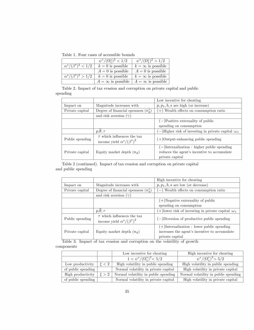
Table 1. Four cases of accessible bounds

s=(s1)2 < 1=2 s=(s1)

2 > 1=2�s=(�s)2 < 1=2 k = 0 is possible k =1 is possible

A = 0 is possible A = 0 is possible�s=(�s)2 > 1=2 k = 0 is possible k =1 is possible

A =1 is possible A =1 is possible

Table 2. Impact of tax evasion and corruption on private capital and publicspending

Low incentive for cheatingImpact on Magnitude increases with p; p1; b; s are high (or increase)Private capital Degree of �nancial openness (n�d) (+) Wealth e¤ects on consumption ratio

and risk aversion ( )(�)Positive externality of publicspending on consumption

p;�; � (�)Higher risk of investing in private capital :!1Public spending

� which in�uences the tax

income yield �s=(�s)2(+)Output-enhancing public spending

Private capital Equity market depth (nd)(�)Internalization : higher public spendingreduces the agent�s incentive to accumulateprivate capital

Table 2 (continued). Impact of tax evasion and corruption on private capitaland public spending

High incentive for cheatingImpact on Magnitude increases with p; p1; b; s are low (or decrease)Private capital Degree of �nancial openness (n�d) (�) Wealth e¤ects on consumption ratio

and risk aversion ( )(+)Negative externality of publicspending on consumption

p;�; � (+)lower risk of investing in private capital :!1

Public spending� which in�uences the tax

income yield �s=(�s)2(�)Diversion of productive public spending

Private capital Equity market depth (nd)(+)Internalization : lower public spendingincreases the agent�s incentive to accumulateprivate capital

Table 3. Impact of tax evasion and corruption on the volatility of growthcomponents

Low incentive for cheating High incentive for cheating

1 < s=(s1)2< 5=2 s=(

s1)2> 5=2

Low productivity � < 2 High volatility in public spending High volatility in public spendingof public spending Normal volatility in private capital High volatility in private capitalHigh productivity � > 2 Normal volatility in public spending Normal volatility in public spendingof public spending Normal volatility in private capital High volatility in private capital

35

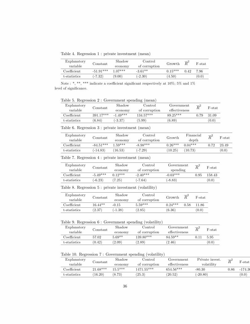
Table 4. Regression 1 : private investment (mean)

Explanatoryvariable

ConstantShadoweconomy

Controlof corruption

Growth R2

F-stat

Coe¢ cient -51.91*** 1.07*** -3.61** 0.15*** 0.42 7.96t-statistics (-7.32) (9.00) (-2.30) (4.50) (0.0)

Note : *, **, *** indicate a coe¢ cient signi�cant respectively at 10%; 5% and 1%level of signi�cance.

Table 5. Regression 2 : Government spending (mean)Explanatoryvariable

ConstantShadoweconomy

Controlof corruption

Governmente¤ectiveness

R2

F-stat

Coe¢ cient 391.17*** -1.49*** 134.57*** 89.25*** 0.79 31.09t-statistics (6.84) (-3.37) (5.99) (6.89) (0.0)

Table 6. Regression 3 : private investment (mean)

Explanatoryvariable

ConstantShadoweconomy

Controlof corruption

GrowthFinancialdepth

R2

F-stat

Coe¢ cient -84.51*** 1.59*** -8.98*** 0.26*** 0.04*** 0.72 23.49t-statistics (-14.83) (16.53) (-7.29) (10.25) (10.73) (0.0)

Table 7. Regression 4 : private investment (mean)

Explanatoryvariable

ConstantShadoweconomy

Controlof corruption

Governmentspending

R2

F-stat

Coe¢ cient -5.49*** 0.12*** -2.40*** -0.03*** 0.95 158.43t-statistics (-6.23) (7.25) (-7.64) (-8.83) (0.0)

Table 8. Regression 5 : private investment (volatility)

Explanatoryvariable

ConstantShadoweconomy

Controlof corruption

Growth R2

F-stat

Coe¢ cient 16.44** -0.15 5.59*** 0.24*** 0.58 11.86t-statistics (2.37) (-1.38) (2.85) (6.36) (0.0)

Table 9. Regression 6 : Government spending (volatility)Explanatoryvariable

ConstantShadoweconomy

Controlof corruption

Governmente¤ectiveness

R2

F-stat

Coe¢ cient 57.02 5.69** 139.80*** 84.59** 0.11 5.95t-statistics (0.42) (2.09) (2.89) (2.46) (0.0)

Table 10. Regression 7 : Government spending (volatility)Explanatoryvariable

ConstantShadoweconomy

Controlof corruption

Governmente¤ectiveness

Private invest.volatility

R2

F-stat

Coe¢ cient 21.68*** 15.5*** 1471.55*** 654.56*** -80.30 0.86 -174.30t-statistics (16.20) (8.73) (25.3) (20.52) (-20.80) (0.0)

36

Table 11. Regression 8 : Growth of per-capita GDPExplanatoryvariable

ConstantPrivate inv(mean)

Gov. spending(mean)

Private inv.(volatility)

Gov.spending(volatility)

Volatility(others)

R2

F-stat

Coe¢ cient -6.05*** 5.59*** 0.68*** -6.05*** -0.76*** 8.40*** 0.99 1202t-statistics (-9.02) (46.50) (38.52) (-15.16) (-84.63) (8.95) (0.0)

37