document classification using machine learning

San Jose State University San Jose State University

SJSU ScholarWorks SJSU ScholarWorks

Master's Projects Master's Theses and Graduate Research

Spring 5-25-2017

DOCUMENT CLASSIFICATION USING MACHINE LEARNING DOCUMENT CLASSIFICATION USING MACHINE LEARNING

Ankit Basarkar San Jose State University

Follow this and additional works at: https://scholarworks.sjsu.edu/etd_projects

Part of the Artificial Intelligence and Robotics Commons, and the Databases and Information Systems

Commons

Recommended Citation Recommended Citation Basarkar, Ankit, "DOCUMENT CLASSIFICATION USING MACHINE LEARNING" (2017). Master's Projects. 531. DOI: https://doi.org/10.31979/etd.6jmu-9xdt https://scholarworks.sjsu.edu/etd_projects/531

This Master's Project is brought to you for free and open access by the Master's Theses and Graduate Research at SJSU ScholarWorks. It has been accepted for inclusion in Master's Projects by an authorized administrator of SJSU ScholarWorks. For more information, please contact [email protected].

https://scholarworks.sjsu.edu/

https://scholarworks.sjsu.edu/etd_projects

https://scholarworks.sjsu.edu/etd

https://scholarworks.sjsu.edu/etd_projects?utm_source=scholarworks.sjsu.edu%2Fetd_projects%2F531&utm_medium=PDF&utm_campaign=PDFCoverPages

http://network.bepress.com/hgg/discipline/143?utm_source=scholarworks.sjsu.edu%2Fetd_projects%2F531&utm_medium=PDF&utm_campaign=PDFCoverPages



https://scholarworks.sjsu.edu/etd_projects/531?utm_source=scholarworks.sjsu.edu%2Fetd_projects%2F531&utm_medium=PDF&utm_campaign=PDFCoverPages

mailto:[email protected]

Ankit Basarkar

DOCUMENT CLASSIFICATION USING MACHINE LEARNING

Digitally signed by Leonard Wesley (SJSU) DN: cn=Leonard Wesley (SJSU), o=San Jose State University, ou, [email protected], c=US Date: 2017.05.24 14:33:30 -07'00'

Dr. Leonard Wesley

Robert Chun Digitally signed by Robert Chun DN: cn=Robert Chun, o=San Jose State University, ou=Computer Science, [email protected], c=US Date: 2017.05.18 18:01:04 -07'00'

Dr. Robert Chun

05/18/2017

Robin James Digitally signed by Robin James Date: 2017.05.18 18:31:05 -07'00'

05/24/2017

05/18/2017Mr. Robin James


A Project Report

Presented to

The Department of Computer Science

San Jose State University

In Partial Fulfillment

of the Requirements for the

Computer Science Degree

by

ANKIT BASARKAR

MAY 2017

http://www.sjsu.edu/

© 2017

Ankit Basarkar

ALL RIGHTS RESERVED

3

The Designated Project Report Committee Approves the Project Report Titled


by

ANKIT BASARKAR

APPROVED FOR THE DEPARTMENT OF COMPUTER SCIENCE

SAN JOSE STATE UNIVERSITY

MAY 2017

Dr. Leonard Wesley Signature: ______________________________

Department of Computer Science

Dr. Robert Chun Signature: ______________________________

Department of Computer Science

Mr. Robin James Signature: ______________________________

Software Developer at BDNA Corp.

REPORT ON DOCUMENT CLASSIFICATION USING MACHINE LEARNING

4

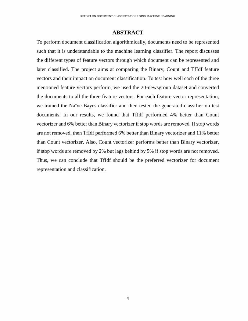
ABSTRACT

To perform document classification algorithmically, documents need to be represented

such that it is understandable to the machine learning classifier. The report discusses

the different types of feature vectors through which document can be represented and

later classified. The project aims at comparing the Binary, Count and TfIdf feature

vectors and their impact on document classification. To test how well each of the three

mentioned feature vectors perform, we used the 20-newsgroup dataset and converted

the documents to all the three feature vectors. For each feature vector representation,

we trained the Naïve Bayes classifier and then tested the generated classifier on test

documents. In our results, we found that TfIdf performed 4% better than Count

vectorizer and 6% better than Binary vectorizer if stop words are removed. If stop words

are not removed, then TfIdf performed 6% better than Binary vectorizer and 11% better

than Count vectorizer. Also, Count vectorizer performs better than Binary vectorizer,

if stop words are removed by 2% but lags behind by 5% if stop words are not removed.

Thus, we can conclude that TfIdf should be the preferred vectorizer for document

representation and classification.


5

ACKNOWLEDGEMENTS

This project work could not have been possible without the help of friends,

family members and the instructors who have supported me and guided me throughout

the project work.

I would like to specifically thank my project advisor, Dr. Leonard Wesley for

guiding me through the course of project work. This project could not have been

possible without his continuous efforts and his wisdom. Also, I would like to mention

along with his support; it was his pure perseverance that pushed me to perform better

during the project that significantly contributed towards its completion on schedule.

I would also like to thank the members of the Committee, Dr. Robert Chun

and Mr. Robin James for their continuous guidance and support. It gives you great

encouragement when you know that there are people whom you can reach out to

whenever you get stuck at something.

Finally, I would like to thank my parents Mr. Shirish Basarkar and Mrs.

Arpita Basarkar, family members, and friends for their perennial encouragement and

emotional support.


6

TABLE OF CONTENTS

1 INTRODUCTION OF DOCUMENT CLASSIFICATION ................................. 10

2 LITERATURE REVIEW OF DOCUMENT CLASSIFICATION ...................... 12

2.1 Classification of Text Documents .................................................................. 12

2.2 Text Categorization with SVM: Learning with Many Relevant Features ..... 15

2.3 Document Classification with Support Vector Machines .............................. 17

2.4 Document Classification for Focused Topics ................................................ 20

2.5 Feature Set Reduction for Document Classification Problems ...................... 21

2.6 Web document classification by keywords using random forests ................. 22

2.7 Support Vector Machines for Text Categorization ........................................ 25

2.8 Enhancing Naive Bayes with Various Smoothing Methods for Short Text

Classification ............................................................................................................ 27

3 RESEARCH HYPOTHESIS AND OBJECTIVES .............................................. 29

4 EXPERIMENTAL DESIGN ................................................................................ 31

4.1 Experiment A Design: Removal of Headers/Footers .................................... 31

4.2 Experiment B Design: Removal of Stop words ............................................ 31

4.3 Experiment C Design: Stemming of words .................................................... 31

4.4 Experiment D Design: Feature representation using Inverse Document

Frequency ................................................................................................................. 32

4.5 Experiment E Design: Naïve Bayes Classifier Training ................................ 32

4.6 Experiment F Design: Addition of Smoothing .............................................. 32

5 APPROACH AND METHOD .............................................................................. 32

5.1 Data Set Exploration ...................................................................................... 32

5.2 Loading Data Set ............................................................................................ 33

5.3 Cleaning of Data Set ....................................................................................... 34

5.4 Vocabulary Generation, Stop words removal and Stemming ........................ 34

5.5 Feature Representation of Documents ........................................................... 36

5.5.1 Binary Vectorizer..................................................................................... 36

5.5.2 Count Vectorizer ...................................................................................... 36


7

5.5.3 TfIdf Vectorizer ....................................................................................... 37

5.6 Classification .................................................................................................. 38

5.7 Testing and Smoothing ................................................................................... 38

6 RESULT ................................................................................................................ 39

7 DISCUSSION OF RESULTS ............................................................................... 43

8 CONCLUSION AND FUTURE WORK .............................................................. 44

9 PROJECT SCHEDULE ........................................................................................ 45

REFERENCES ............................................................................................................. 47

APPENDICIES ............................................................................................................ 49


8

List of Figures

Figure 1: An example of the business news group: (a) a training sample; (b) extracted

word list ........................................................................................................................ 13

Figure 2: Document Classification using SVM ........................................................... 18

Figure 3 : Two-dimensional representation of documents in 2 classes separated by a

linear classifier. ............................................................................................................ 19

Figure 4 : Artificial Neural Net .................................................................................... 26


9

List of Tables

Table 1: Comparison of the four classification algorithms (NB, NN, DT and SS) 15

Table 2: Classification accuracies of combinations of multiple classifiers 15

Table 3: Precision/recall-breakeven point on the ten most frequent Reuters categories

and micro averaged performance over all Reuters categories. 17

Table 4 : Classification Accuracy of Standard Algorithms 21

Table 5 : Topic classification rates with random forests for 7 topics 24

Table 6 : Topic classification rates with other algorithms for 5 topics 24

Table 7 : Topic classification rates with other algorithms for 7 topics 24

Table 8 : Test Data Summary 27

Table 9 : Macro Averaging Results 27

Table 10 : Categories of Newsgroup Data Set 33

Table 11 : Comparison of Results 41

Table 12 : Classification report of Test Documents using TfIdf Vectorizer and Naive

Bayes Classifier 42

Table 13 : Schedule employed for Project 45


10

1 INTRODUCTION OF DOCUMENT CLASSIFICATION

Document classification is the task of grouping documents into categories based

upon their content. Document classification is a significant learning problem that is at

the core of many information management and retrieval tasks. Document classification

performs an essential role in various applications that deals with organizing, classifying,

searching and concisely representing a significant amount of information. Document

classification is a longstanding problem in information retrieval which has been well

studied [4].

Automatic document classification can be broadly classified into three

categories. These are Supervised document classification, Unsupervised document

classification, and Semi-supervised document classification. In Supervised document

classification, some mechanism external to the classification model (generally human)

provides information related to the correct document classification. Thus, in case of

Supervised document classification, it becomes easy to test the accuracy of document

classification model. In Unsupervised document classification, no information is

provided by any external mechanism whatsoever. In case of Semi-supervised document

classification parts of the documents are labeled by an external mechanism [10].

There are two main factors which contribute to making document classification

a challenging task: (a) feature extraction; (b) topic ambiguity. First, Feature extraction

deals with taking out the right set of features that accurately describes the document

and helps in building a good classification model. Second, many broad topic documents

are themselves so complicated that it becomes difficult to put it into any specific

category. Let us say a document that talks of about theocracy. In such document, it

would become tough to pick whether the document should be placed under the category

of politics or religion. Also, broad topic documents may contain terms that have

different meanings based on different context and may appear multiple times within a

document in different contexts [4].


11

Never before has document classification been as imperative as it is at the

moment. The expansion of the internet has resulted in significant increase of

unstructured data generated and consumed. Thus there is a dire need for content-based

document classification so that these documents can be efficiently located by the

consumers who want to consume it. Search engines were precisely developed for this

job. Search engines like Yahoo, HotBot, etc. in their early days used to work by

constructing indices and find the information requested by the user however it was not

very uncommon that search engines at times may return a list of documents with poor

correlation. This has led to development and research of intelligent agents that makes

use of machine learning in classifying documents.

Some of the techniques that are employed for document classification include

Expedition maximization, Naïve Bayes classifier, Support Vector Machine, Decision

Trees, Neural Network, etc.

Some of the applications that make use of the above techniques for document

classification are listed below:

Email routing: Routing an email to a general address, to a specific address or

mailbox depending on the topic of the email.

Language identification: Automatically determining the language of a text.

It can be useful in many use cases one of them being the direction in which

the language should be processed. Most of the languages are read and written

from left to right and top to bottom, but there are some exceptions though.

For example, Hebrew and Arabic are processed from right to left. This

knowledge can then be used along with language identification in correct

processing of the text in any language.

Readability assessment: Automatically determining how readable any

document is for an audience of a certain age.


12

Sentiment analysis: Determining the sentiment of a speaker based on the

content of the document [10].

2 LITERATURE REVIEW OF DOCUMENT CLASSIFICATION

This topic discusses the work done by various authors, students and researchers

in brief in the area under discussion, which is Document Classification using Machine

Learning algorithms. The purpose of this section is to critically summarize the current

knowledge in the field of document classification.

2.1 Classification of Text Documents

Introduction: In the work [1] done by Y. H. LI AND A. K. JAIN they

performed document classification on the seven class Yahoo newsgroup data set. The

data set contained documents divided into following classes: International, Politics,

Sports, Business, Entertainment, Health, and Technology.

They employed Naïve Bayes, Decision Trees, Nearest neighbor classifier and

the Subspace method for classification. They also performed classification using the

combination of these algorithms.

Feature representation: They adopted the commonly used bag of words

document representation scheme for feature representation. They ignored the structure

of document and arrangement of words in their feature representation. The feature

vectors contained all the distinct words in the training set after removal of all the stop

words. The stop words are the words that do not help in document classification such

as ‘the,' ‘and,' ‘some,' ‘it,' etc. They also removed some of the low-frequency words

that occur very seldom in the training set of documents.

In a general scenario, there will be thousands of features (given a large volume

of documents in your dataset) since there are around 50,000 commonly used words in

the English language. Given a document D, its feature vector is generated. For creating


13

the feature vector for each document, they made use of 2 approaches. The first is the

binary approach where for each word in vocabulary the value of 1 is given if the word

exists in the document D or 0 if it does not. In the second approach, the frequency of

each word is used to form a feature vector.

In this paper, they used a Binary representation for Naïve Bayes and Decision

trees method. Whereas, they used Frequency representation in Nearest neighbor

classifier and the Subspace method classifier to calculate the weight of each term.

Figure 1: An example of the business newsgroup: (a) a training sample;

(b) extracted word list

Combination of multiple classifiers: Apart from the application of the

mentioned four algorithms the authors also tried the combination of algorithms to see

if they can improve the model being designed. They used Simple voting, DCS

(Dynamic classifier selection) and ACC (Adaptive classifier combination) for

combining the individual methods to create a classification model.


14

Simple voting is one of the simplest combination approaches. In simple voting,

each document is classified to a certain category by each of the four classifiers. The

combination selects the class that is selected by majority of the classifiers.

In DCS (Dynamic classifier selection) approach, the authors found the

neighborhood of document D by using k-nearest neighbor approach. After this, they

employed leave one out method on training data to find the local accuracy of the

classifier.

In ACC (Adaptive classifier combination) a classifier with maximum local

accuracy is chosen to predict the class for test document. Thus, the class chosen by the

classifier with maximum local accuracy is chosen by the ACC.

Data Set and Experiments: The authors preprocessed the documents by

removing HTML tags, stop words and words with low frequency. The authors used 814

documents of the Yahoo newsgroup data set that were divided across seven categories

for training the classifier.

To test the classifiers, they used, two different test data sets taken at different

time intervals. The authors first tested all the four machine learning algorithms

individually on both the test data sets. Then they tested the three combinations on both

the test data sets.

In their experiments, all the four machine learning algorithms performed well.

The naïve bayes gave the highest accuracy for first test data set but was outperformed

by subspace method for the second test data set.


15

Table 1: Comparison of the four classification algorithms (NB, NN, DT

and SS)

After the application of individual algorithms, the authors also performed

analysis using a combination of these algorithms. The results of some of such

combinations are illustrated in the figure below.

Table 2: Classification accuracies of combinations of multiple classifiers

Conclusion: The authors concluded that all the four classifiers performed

reasonably well on the Yahoo data-set. From the four algorithms, the Naive Bayes

method gave the highest accuracy. The authors also noticed that combination of

classifiers does not guarantee much improvement over the individual classifier.

2.2 Text Categorization with SVM: Learning with Many Relevant Features

Introduction: In this paper [2] the author Thorsten Joachims explored and

identified the benefits of Support Vector Machines (SVMs) for text categorization.

Feature Representation: The author performed stemming as part of

preprocessing before creating the feature vectors. For generating feature vectors, the


16

authors made use of word counts. Thus each document was represented as vector of

integers where each integer represented the number of times a corresponding word

occurred in the document. To avoid large feature vectors the author only considered

those words as features that took place more than three times in the document. The

authors also made sure to eliminate stop words in making feature vectors.

This representation scheme still led to very high-dimensional feature spaces

containing 10000 dimensions and more. To reduce the number of features and

overfitting, information gain criterion was used. Thus only a subset of features was

selected based on Information gain.

Data Set and Experiments: The author used two data sets for the model. The

first data set author used was ModApte split of the Reuters-21578 dataset which is

compiled by David Lewis. This dataset contained 9603 training documents and 3299

test documents. The dataset contained 135 categories of which only 90 were used since

only 90 categories had at least one training and test sample.

The second data set employed for model creation and evaluation was the

Ohsumed corpus which was compiled by William Herse. The author used 10000

documents for training and another 10000 for testing from the corpus that had around

50000 documents. The classification task on this data set was to assign each document

to one of the 23 MeSH diseases category.

The author compared the performance of SVMs with Naïve Bayes, Rocchio,

C4.5, and KNN for text categorization. The author used polynomial and RBF kernels

for SVM. The Precision/Recall Breakeven Point is used as a measure of performance

and micro-averaging is done to get a single value of performance for all classification

tasks. The author also ensured that the results are not biased towards any particular

method and thus he ran all the four methods after selecting the best 500, best 1000, best

2000, best 5000 or all features based on Information gain.


17

Table 3: Precision/recall-breakeven point on the ten most frequent

Reuters categories and micro-averaged performance over all Reuters categories.

Conclusion: The author concludes that, among the conventional methods KNN

performed the best on Reuters data set. On the other hand, SVM achieved the best

classification results and outperformed all the conventional methods by a good margin.

The author states that SVM can perform well in high dimensional space and thus does

not mandate feature selection which is almost always required by other methods. The

author also concludes that SVMs are quite robust and performed well in virtually all

experiments.

The author observed similar results for the Ohsumed collection data set as well.

The results demonstrated that k-NN performed the best among conventional methods

whereas SVM outperformed all the other conventional classifiers.

2.3 Document Classification with Support Vector Machines

Introduction: In the paper [3] written by Konstantin Mertsalov and Michael

McCreary they discuss the implementation of Support Vector Machine for Document

Classification. SVM is a group of learning algorithms that are primarily used for

classification tasks on complex data such as image classification and protein structure


18

analysis. This paper mainly deals with why we need Automatic Document classification

is in a way like the motivation posted above regarding Document Classification by

Machine Learning. This paper covers the inner workings of Support Vector Machine,

its application in the classification and its accuracy compared to manual classification.

Thus, in a way this paper is an extension to the motivation illustrated above regarding

why we need document classification using machine learning.

The Classifier Model: A typical approach of classification employed by SVM

is shown in figure 2. The SVM model is trained against a labeled set of documents. The

model is then validated using another set of labeled documents. Once the validation is

done and the error observed is within threshold the model is considered fit for

classification of unseen and unlabeled documents.

Figure 2: Document Classification using SVM

In the training phase of SVM, the algorithm is fed with labeled documents of

both categories. Internally SVM converts all the documents into a data point in high-

dimensional space. These points represent the documents. Then the algorithm tries to


19

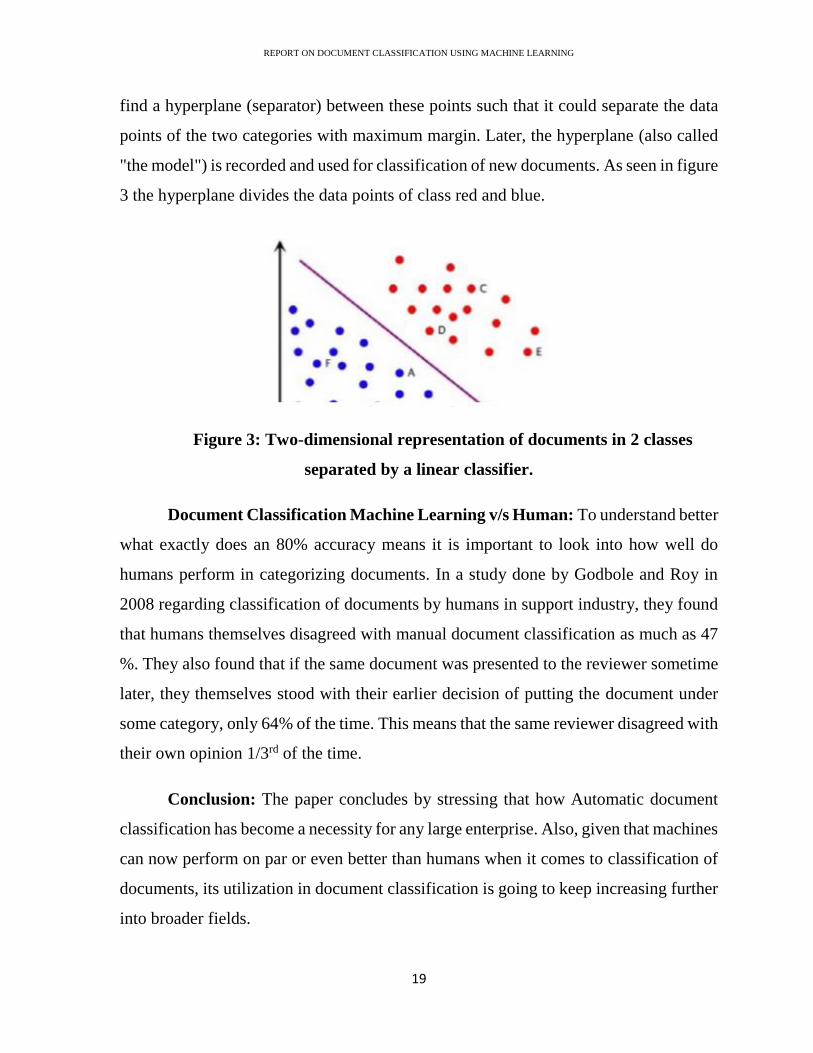
find a hyperplane (separator) between these points such that it could separate the data

points of the two categories with maximum margin. Later, the hyperplane (also called

"the model") is recorded and used for classification of new documents. As seen in figure

3 the hyperplane divides the data points of class red and blue.

Figure 3: Two-dimensional representation of documents in 2 classes

separated by a linear classifier.

Document Classification Machine Learning v/s Human: To understand better

what exactly does an 80% accuracy means it is important to look into how well do

humans perform in categorizing documents. In a study done by Godbole and Roy in

2008 regarding classification of documents by humans in support industry, they found

that humans themselves disagreed with manual document classification as much as 47

%. They also found that if the same document was presented to the reviewer sometime

later, they themselves stood with their earlier decision of putting the document under

some category, only 64% of the time. This means that the same reviewer disagreed with

their own opinion 1/3rd of the time.

Conclusion: The paper concludes by stressing that how Automatic document

classification has become a necessity for any large enterprise. Also, given that machines

can now perform on par or even better than humans when it comes to classification of

documents, its utilization in document classification is going to keep increasing further

into broader fields.


20

2.4 Document Classification for Focused Topics

Introduction: In the paper [4] written by Russell Power, Jay Chen, Trishank

Karthik and Lakshminarayanan Subramanian, they propose a combination of feature

extraction and classification algorithms for classification of documents. In this paper,

they propose a simple feature extraction algorithm for development centric topics which

when coupled with standard classifiers yields high classification accuracy.

Popularity and Rarity: In this paper, they propose a simple feature extraction

algorithm for development centric topics which when coupled with standard classifiers

yields high classification accuracy.

There features extraction algorithm made use of a combination of two

completely different and potentially opposing metrics, for the purpose of extracting

textual features for a given topic: (a) popularity; (b) rarity.

The popularity of words can be described as how popular a word is for a certain

category of documents. For a given set of documents this metric determines a list of

words that occur most frequently in the document and is closely related to the topic.

The rarity metric, on the other hand, captures the list of least frequent terms that

are closely related to the topic. They leveraged the Linguistic Data Consortium (LDC)

data set to learn the frequency of occurrence of any n-gram on the Web to measure

rarity of any given term. Although the LDC data set that they used is slightly old, they

found that in a separate study it was observed that the rarity of terms with respect to

any category is preserved and the relation does not become obsolete.

Data Set and Experiments: The dataset they used for classification was the “4

University” set from WebKB. The data set contained pages from several universities

that were then grouped into seven categories namely: student, course, staff, faculty,

department, project and other. Since there can be ambiguity among some of the


21

categories, classification often is performed on a subset of the documents consisting of

the student, faculty, staff and course groups.

To achieve good classification accuracy, they exploited both popularity and

rarity metrics for feature extraction. Either one by themselves does not provide enough

accuracy as has been proven by other researchers in their prior study. In addition to

limiting the size of the feature set by using these two metrics, they were also able to

minimize the noise in the feature set. For example, if a document is large, it will have

a large set of features; which may make the document to be likely classified into

multiple classes. Thus, reducing the feature set thereby limiting the noise greatly

benefits the process of classification.

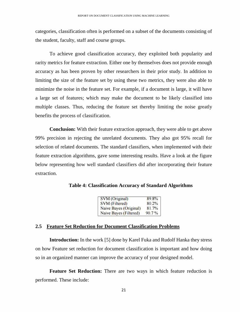
Conclusion: With their feature extraction approach, they were able to get above

99% precision in rejecting the unrelated documents. They also got 95% recall for

selection of related documents. The standard classifiers, when implemented with their

feature extraction algorithms, gave some interesting results. Have a look at the figure

below representing how well standard classifiers did after incorporating their feature

extraction.

Table 4: Classification Accuracy of Standard Algorithms

2.5 Feature Set Reduction for Document Classification Problems

Introduction: In the work [5] done by Karel Fuka and Rudolf Hanka they stress

on how Feature set reduction for document classification is important and how doing

so in an organized manner can improve the accuracy of your designed model.

Feature Set Reduction: There are two ways in which feature reduction is

performed. These include:


22

Feature selection: In this approach, a subset of original features is retained

while the rest are discarded. The classification model is then built using the

selected features. The aim is to select such features that result in high

accuracy classifier.

Feature extraction: In this feature reduction technique the original vector

space is transformed to form a new minimalistic feature vector space. Unlike

Feature selection technique, in this method, all the features are used. The

original features are transformed into a smaller set of transformed features

which might not be meaningful to humans but are composed of original

human understandable features.

Both of these approaches require optimization of some criterion function J,

which is usually a measure of distance or dissimilarity between distributions.

Data Set and Experiments: The authors used “Reuters-21578” dataset for

training and testing the classifier. Some of the feature reduction techniques employed

by the authors were chi-squared statistic and PCA. The authors started with 3822

original terms in the beginning. The authors used χ 2 statistical data for feature selection

that gave an accuracy of approx. 81%. The authors used PCA to test feature extraction.

PCA, when applied to features obtained through χ 2 statistic, gave an accuracy of 86%

and PCA when applied over the complete feature set provided an accuracy of 95%

Conclusion: The authors concluded that all feature set reduction algorithms

perform better compared to no feature reduction. Also, appropriate feature extraction

algorithm can perform better than feature selection algorithm.

2.6 Web document classification by keywords using random forests

Introduction: In the paper [6] Myungsook Klassen and Nikhila Paturi present a

comparative study of web document classification. The author's prime focus for the

study was on the random forest. Apart from the random forest, the authors also used


23

Naïve Bayes, Multilayer perceptron, RBF networks and regression for classification.

The authors also studied the effect of the addition of topics to the accuracy of the model.

To test this, they performed experiments on data set containing 5 topics and 7 topics.

Random Forest: The Random forest is a statistical method for classification.It

was first introduced in 2001 by Leo Breiman. It is a decision-tree based supervised

learning algorithm. The Random forest consists of many individual decision trees. Each

decision tree votes for classification of given data. The random forest algorithm then

accepts the classification which got a maximum number of votes from individual trees.

Collectively the decision tree models represent or form a random forest where each

decision tree votes for the result and the majority wins.

Data Set: The authors used Dmoz Open Directory Project (ODP) data set for

their experiments. The data set contains pre-classified web documents that are part of

the open content directory. The directory uses hierarchical ordering where each

document is listed in a category based on its content. The authors used 5 and 7

categories for their experimentations.

Preprocessing: As a first step of preprocessing, the authors removed all the

HTML tags from the web document. After this, the author removed all the stop words

from the document. Stop words are common English words like ‘the,' ‘a,' ‘to’ etc. that

do not help in classification, since they occur across all documents irrespective of the

category to which the documents belong. The authors after stop words removal

performed stemming. The authors after this used bag of words approach to represent

the documents in terms of term frequency. To minimize the size of vocabulary, the

authors dropped those terms from adding to vocabulary that occurred less than 5 times

in a document. After this the authors selected 20 most occurring words in a document

for its representation.

Experiments: In the first experiment, the authors analyzed the role of number

of trees (“numTrees”) and number of features (“numFeatures”) of random forest. The


24

authors used the tree depth of 0, that is the tree was allowed to grow as deep as possible.

The authors used 20, 30 and 40 number of trees in the random forest. 0 to 60 number

of features were used to test the classifier to detect which setting gives the highest

accuracy. For this experiment, the authors got the highest accuracy of 83.33% when the

number of trees was 20 and number of features were 50. They got this accuracy for 5

topics. For 7 topics, the best classification accuracy dropped to 80.95 % with 40 trees

and 35 features.

Table 5: Topic classification rates with random forests for 7 topics

As a second experiment, the authors of the paper performed document

classification using different algorithms for both 5 topics and 7 topics. The results of

them are shared below.

Table 6: Topic classification rates with other algorithms for 5 topics

Table 7: Topic classification rates with other algorithms for 7 topics


25

Conclusion: The authors concluded that even though other machine learning

algorithms performed well, random forest outperformed all the other algorithms. Also,

as the number of topics increased the accuracy of the other algorithms declined steeply

compared to the random forest. The authors also found that some of the other algorithms

were not scalable as well. For instance, the multilayer perceptron was performing ten

times slower than all the other algorithms.

2.7 Support Vector Machines for Text Categorization

Introduction: In the paper [7], the authors A. Basu, C. Watters, and M.

Shepherd compared support vector machine with an artificial neural network for the

purpose of text classification of news items.

Data Set: The authors used Reuters News data set for their comparative study.

As the name suggests, the Reuters-21578 dataset contains a collection of 21,578 news

items that are divided across 118 categories.

SVM: These are set of binary classification algorithms proposed by Vapnik. It

works by finding a hyperplane that separates the two classes with maximum margin.

SVM can operate with a large feature set without much feature reduction. This makes

SVM an accomplished algorithm for classification.

ANN: Artificial Neural Network imitates the actual working of neurons in the

human brain. In ANN, an impulse is modeled by a vector value, and change of impulse

is modeled using transfer function. A sigmoid, stepwise or even a linear function is

considered as a transfer function.


26

Figure 4 : Artificial Neural Net

Data Set Preprocessing: The authors converted the SGML documents into

XML documents using the SX tool. The authors removed the documents that belonged

to no category or belonged to multiple categories. After this, the authors removed the

categories that had less than 15 documents left in it. The elimination left 63 categories

containing 11,327 documents.

Vocabulary: After preprocessing of data set, an extensive vocabulary of

102,283 terms was generated using KSS (Knowledge System Server). To limit the size

and complexity of vocabulary, the authors used two different IQ values. The KSS with

IQ value of 87 resulted in the vocabulary of 62,106 terms and IQ value of 57 resulted

in 78,165 terms. The figure of 78,165 was further reduced to 33,191 by removal of

abbreviations and terms not understandable by the KSS.

Experimentation: To test both the classifiers, authors chose 600 documents

from the pool at random. Since the draw was random, many times, they were left with

a set of documents that had too few or no documents from some of the categories. Thus,

apart from testing for all the categories they also did testing for only those categories

that had more than ten documents in the random 600 document test pool.


27

Table 8 : Test Data Summary

Table 9 : Macro Averaging Results

Conclusion: After experiments, the authors concluded that SVM performed

much better than Artificial Neural Network for both IQ87 and IQ57. Since SVM is also

less computationally expensive, the authors recommended SVM over ANN for data set

containing fewer categories with short documents.

2.8 Enhancing Naive Bayes with Various Smoothing Methods for Short Text

Classification

Introduction: In the work [8] done by Quan Yuan, Gao Cong and Nadia M.

Thalmann they experimented with the application of various smoothing techniques in

implementing the Naïve Bayes classifier for short text classification.

Naïve Bayes: In this time, millions of new documents get generated and

published every second. Hence, it is important that the employed classification method

be able to accommodate the new training data efficiently and to classify a new text

efficiently. The Naive Bayes (NB) method is known to be a robust, effective and

efficient technique for text classification. More importantly, it can accommodate new

incoming training data in classification models incrementally and efficiently.


28

Smoothing: Given a question d to be classified, Naive Bayes (NB) assumes that

the features are conditionally independent and finds the class ci that maximizes

p(ci)p(d|ci).

where |ci| is the number of questions in ci, and |C| is the total number of questions in the

collection. For NB, likelihood p(wk|ci) is calculated by Laplace smoothing as follows:

where c(w, ci) is the frequency of word w in category ci, and |V| is the size of

vocabulary. For different smoothing methods, p(wk|ci) will be computed differently.

We consider the following four smoothing methods used in language models for

information retrieval. Let c(w, ci) denote the frequency of word w in category ci, and

p(w|C) be the maximum likelihood estimation of word w in collection C.

Jelinek-Mercer (JM) smoothing:

Dirichlet (Dir) smoothing:

Absolute Discounting (AD) smoothing:

where δ ∈ [0, 1] and |ci|u is the number of unique words in ci.

Two-stage (TS) smoothing:


29

Data Set and Experimentation: They used Yahoo! Webscope dataset that

comprises of 3.9M questions belonging to 1,097 categories (e.g., travel, health) from a

Community-based Question Answering (CQA) service, as an example of short texts, to

study question topic classification.

They extracted 3,894,900 questions from Yahoo! Webscope dataset. They

removed stop words and did stemming. Additionally, they deleted the words that occur

less than 3 times in the dataset to reduce misspelling.

They randomly selected 20% questions from each category of the whole dataset

as the test data. From the remaining 80% data, they generated 7 training data sets with

sizes of 1%, 5%, 10%, 20%, 40%, 60%, and 80% of the whole data, respectively. They

applied the smoothing algorithms discussed before and did a comparative study.

Conclusion: The authors applied various smoothing algorithms while

conducting classification with Naïve Bayes. The experimental results obtained by the

authors show

Smoothing methods were able to significantly improve the accuracy of

Naive Bayes for short text classification.

Among the four smoothing methods, Absolute Discounting (AD) and

Two-stage (TS) performed the best.

3 RESEARCH HYPOTHESIS AND OBJECTIVES

The purpose of the project work that we did was to determine, what is the best

way in which features of documents could be represented, to achieve improved

document classification accuracy.


30

For the objective mentioned above, We studied about how count vectorizer

works and how term frequency is evaluated for each document. We also studied how

to represent each document in the form of sparse matrix purely based on the term

frequency. We noted a flaw with this representation. The flaw is, irrespective of how

common or rare the word is we calculate just the frequency of a certain word in each

document. Thus, we assign a value to the feature of the document ( a feature in our case

being a word) purely based on how many times it occurs. We do not take into account

how much distinguishing the word is. To elaborate on this further let us put forward a

simple example.

Let us say we have a document that contains a word ‘catch’ 10 times and the

word ‘baseball’ 2 times. Here, if we just used term frequency, we will give more weight

to the word ‘catch’ compared to the word ‘baseball’ since it occurs more frequently in

the document. However, the word ‘catch’ might frequently be occurring across multiple

categories whereas the word ‘baseball’ might be occurring in very few categories that

are related to sports or baseball. Thus, the word ‘baseball’ is a more distinguishing

feature in the document. In inverse document frequency, we determine the

distinguishability of the word which we then multiply with term frequency to get the

new weight of each word in the document.

As seen in the previous example if we ignore the distinguishability of words in

the document and weigh the term frequency alone, we might not be able to predict the

class of the document accurately. Thus, considering the inverse document frequency

along with term frequency should help in better document classification. Based on this

knowledge I would like to posit my Null and Alternative Hypothesis.

Alternative Hypothesis: Considering inverse document frequency along with

term frequency for feature representation of each document to conduct document

classification should result in accuracy improvement of the document classification

model by up to 5 percent.


31

Null Hypothesis: Considering inverse document frequency along with term

frequency for feature representation of each document to conduct document

classification will not be able to improve accuracy of the document classification model

by 5 percent.

4 EXPERIMENTAL DESIGN

4.1 Experiment A Design: Removal of Headers/Footers

Since all the documents of the dataset contain headers/footers such as From,

Subject, etc. Elimination of these from the actual content of the document can lead to

better classification.

4.2 Experiment B Design: Removal of Stop words

Almost all the documents across all categories contain words like ‘The,' ‘A,'

‘From,' ‘To,' etc. These words might hamper the classification task and might make

the classification results skewed. Removal of these words may give more accurate

classification results.

4.3 Experiment C Design: Stemming of words

Some of the words originate from another word. In such cases, it would be

better if we consider all form of root words as the root word itself. Let us say we have

the following words with frequency in a given document; walk: 3, walked: 4,

walking: 6. Thus instead of considering all the three forms separately, we can

consider the root word walk with the frequency of 13 since all the three words signify

the same meaning in a different tense. Stemming of words before feature

representation can lead to better classification accuracy.


32

4.4 Experiment D Design: Feature representation using Inverse Document

Frequency

This is one of the most important experiments of the project work and core of

the hypothesis posited above. The count vectorizer considers the frequency of words

occurring in document irrespective of distinguishability of words in a document for

feature representation of documents. Instead, the documents could be better represented

if we consider the term frequency along with how much distinguishing the term is. Such

representation should also help improve the overall accuracy of the model.

4.5 Experiment E Design: Naïve Bayes Classifier Training

After getting the feature representation of all documents, the classifier is trained

on the training set of documents (feature vectors of training documents).

4.6 Experiment F Design: Addition of Smoothing

As mentioned earlier, Smoothing is one of the important factors in building

Naïve Bayes classifier model. The addition of smoothing should help in the better

handling of unknowns while testing the classification model.

5 APPROACH AND METHOD

This part of the report illustrates the approach employed by me to do document

classification.

5.1 Data Set Exploration

The first step of our research/project work was determining the right data set.

We came across many data sets like Reuters data set and Yahoo data set. We selected

the 20 Newsgroup dataset collected by Ken Lang for our task. We selected this data

set because of several reasons. The reasons include: a) The data set is large, so working

with it is intriguing; b) The number of categories in the data set is 20 as opposed to

most of the data sets containing binary categories; c) The number of documents is quite

evenly divided among the 20 categories.


33

Organization: The data set has 20 categories of which some categories are very

closely related like the category of ‘talk.religion.misc’ and ‘soc.religion.christian'

Whereas some categories are entirely distinct like ‘rec.sport.baseball’ and ‘sci,space.'

The below table illustrates all the categories that comprise the data set.

Table 10: Categories of Newsgroup Data Set

The dataset is available to download at [9].

5.2 Loading Data Set

Unlike other data sets that are generally CSV files containing a comma separated

values, which can be loaded easily, the task of loading the data set was a bit convoluted.

The data set contained two primary folders named as ‘train’ and ‘test.' Each folder

further contained 20 folders, one for each category of documents. Inside these folders

were the actual documents. Each category contained around 600 train documents and

around 400 test documents.

All the train documents were loaded into a single Bunch object which contained

the actual documents in a list. The Bunch object for train data also contained a list of

length equal to the length of documents list, containing the corresponding category of

each document. The Bunch object also contained a map object that maps the category

that is a string with an integer literal, thus representing category with an integer. All the

documents being added to the Bunch object is also shuffled to distribute them evenly


34

across categories when added to the list. Similarly, a Bunch object for Test data set was

also created.

5.3 Cleaning of Data Set

Before the Vocabulary generation and Feature representation of the documents,

headers, and footers of the documents are removed. These include ‘From,' ‘Subject,'

‘Organization,' ‘Phone,' ‘Fax’ etc. Removal of these leaves us with the actual content

of the document and the category to which it belongs. This helps us in limiting the

length of vocabulary (though still huge). Also, these headers and footers do not

contribute in any significant way in helping us achieve our objective, that is

classification of documents based on actual content of documents.

5.4 Vocabulary Generation, Stop words removal and Stemming

After cleaning of the dataset, the next step is the creation of vocabulary.

Vocabulary is set of all words, which occur in training set of documents, at least once.

To better understand the concept, consider an example. Let us say we have two

documents D1 and D2.

D1: “A system of government in which priests’ rule in the name of God is termed as

Theocracy.” – “Christianity.”

D2: “A ball game played between two teams of nine on a field with a diamond-shaped

circuit of four bases is termed as Baseball.” – “Baseball.”

Here the Vocabulary V will be a set containing all words that occur at least once.

The Vocabulary formed will be;

V: {‘A’, ‘system’, ‘of’, ‘government’, ‘in’, ‘which’, ‘priests’’, ‘rule’, ‘the’, ‘name’,

‘God’, ‘is’, ‘termed’, ‘as’, ‘Theocracy’, ‘ball, ‘game’, ‘played’, ‘between’, ‘two’,

‘teams’, ‘nine’, ‘on’, ‘field’, ‘with’, ‘diamond’, ‘shaped’, ‘circuit’, ‘four’, ‘bases’,

‘Baseball’}


35

The problem with such Vocabulary is that it contains many stop words. Stop

words are the common English words that do not help in classification of documents at

all. Let us analyze the Vocabulary we just created. It already contains a lot of stop words

(SW).

SW: {‘A’, ‘of,' ‘in,' ‘which,' ‘the,' ‘is,' ‘as,' ‘on,' ‘with’}

These words have got no relation with either of the two categories and may

appear in all categories whose documents are under investigation. Thus, in Vocabulary

creation, these words will be removed. The stop word removed vocabulary (SWRV)

will contain all the words that occur at least once in the training set of documents except

the stop words. For our example, the stop words removed vocabulary will look like as

shown below.

SWRV: {‘system’, ‘government’, ‘priests’’, ‘rule’, ‘name’, ‘God’, ‘termed’,

‘Theocracy’, ‘ball, ‘game’, ‘played’, ‘between’, ‘two’, ‘teams’, ‘nine’, ‘field’,

‘diamond’, ‘shaped’, ‘circuit’, ‘four’, ‘bases’, ‘Baseball’}

Although SWRV will work better than the simpler V, it still can be improved by

using Stemming. Stemming is the process of converting inflected (changed form) words

to their stem words. Consider, for our example we get another document D3.

D3: “Square is a shape formed by four edges.” – “Geometry.”

Thus, in our SWRC we must add the following words; {‘Square,' ‘shape,'

‘formed,' ‘four,' ‘edges’}. Notice that the word ‘shaped’ already exists in our SWRV.

The stem/root word of ‘shaped’ is ‘shape’ which we are trying to add now. Since both

the word convey the same meaning and come from the same root word, it does not

make sense to keep both in the vocabulary. This addition to the vocabulary could have

been avoided if we had performed stemming. Stemming not just help in limiting the

size of the Vocabulary but also helps in keeping the size of the feature vector in check

which we will see later in the report.


36

5.5 Feature Representation of Documents

This is one of the most important tasks of Document classification. In Feature

representation of documents, documents are converted into feature vectors. There are

many approaches in which this is done.

5.5.1 Binary Vectorizer

One of the simplest being a binary feature vector. In this method, for all the

words in the vocabulary, the words that occur in the document at least once, is counted

positive (1) whereas the words that do not occur is not counted (0). Thus, each

document is represented as a vector of words with values of each word mapped to either

0 (if it does not occur in that document) or 1 (if it does take place in the document).

Since a document may not contain a lot of words that are there in a dictionary,

it will have most of the words in feature vector with value ‘0’. Thus, there is a lot of

storage space wasted. To overcome this limitation, we make use of the sparse matrix.

In the sparse matrix, we store only the words whose value is non-zero, resulting in

significant storage saving.

5.5.2 Count Vectorizer

Though Binary Feature Vector is one of the simplest, it does not perform that

well. It does capture, whether certain words exist in the document but it fails in

capturing the frequency of those words. For this reason, Count vectorizer (also termed

as Term Frequency vectorizer) is generally preferred.

In count vectorizer, we do not just capture the existence of words for a given

document but also capture how many times it occurs. Thus, for each word in a

vocabulary that occurs in a document we capture the number of times it occurs. Thus,

the document is represented as a vector of words along with the number of times it

occurs in the document. For this approach, also Sparse matrix is used since most of the

words in vocabulary will likely have a frequency of ‘0’.


37

5.5.3 TfIdf Vectorizer

The count vectorizer captures more detail than a simpler binary vectorizer, but

it also has a certain limitation. Although count vectorizer considers the frequency of

words occurring in a document, it does it irrespective of how rare or common the word

is. To overcome this limitation TfIdf (Term Frequency Inverse Document Frequency)

vectorizer can be used. TfIdf vectorizer does consider the inverse document frequency

(distinguishability weight of the word) along with the frequency of each word occurring

in a document, in forming the feature vector.

Let us say we have a document that contains a word ‘catch’ 10 times and the

word ‘baseball’ 2 times. Here, if we just used term frequency, we will give more weight

to the word ‘catch’ compared to the word ‘baseball’ since it occurs more frequently in

the document. However, the word ‘catch’ might frequently be occurring across multiple

categories whereas the word ‘baseball’ might be occurring in very few categories that

are related to sports or baseball. Thus, the word ‘baseball’ is a more distinguishing

feature in the document. In inverse document frequency, we determine the

distinguishability of the word which we then multiply with term frequency to get the

new weight of each word in the document. How the TfIdf is calculated is shown below:

TF (Term Frequency) = Number of times term/word occurs in the document.

IDF (Inverse Document Frequency) = log (N/ 1 + {d ϵ D : t ϵ d})

Here, N is a total number of documents in the corpus and {d ϵ D: t ϵ d} is a number of

documents where term t appears. TfIdf is calculated as:

TfIdf = TF * IDF

Thus, if the word occurs less across multiple documents than its

distinguishability or in more technical terms it’s IDF value will be high and the word

that frequently occurs across many documents will have a low IDF value. Thus, in TfIdf


38

the feature vector will not be based solely on term frequency of words but will be a

product of term frequency along with its IDF value.

5.6 Classification

For each kind of representation (Binary Vectorizer, Count Vectorizer, and TfIdf

Vectorizer) a Multinomial Naïve Bayes Classification model is generated. A

multinomial classifier is chosen because the feature set is multinomial in nature, that is

it can take a variable number. The classifier makes use of feature vector, and based on

it, learns to which class the document belongs. Thus, based on the feature vector of all

the training documents along with its target class the machine learning model is trained.

5.7 Testing and Smoothing

After the Classification model is built, the classifier is tested against the set of

test documents that account for 40% of the documents. To test documents that contain

unknown words Laplace smoothing is added.

Naïve Bayes classifier works on the assumption that all features are independent

and thus it takes the multiplicative product of the probabilities of each feature to

determine the likelihood for a given class. Thus, if there is any word that occurs in the

test document but is not a part of vocabulary (that is it never occurred in the training

document), then the probability of that feature will become 0. Since in Naive Bayes

multiplication of probabilities is done, because of probability of a single feature being

0 the complete result will become 0. Thus, even if the test document had significant and

discriminating features their result would be lost, and the document will become

Uncategorized with the likelihood of 0.

To understand this better consider a simple case of binary classification between

ham and spam emails. Let us say we trained our naïve bayes classifier on a training set

of documents. We get a test document TD1

TD1: You won billion in Lottery.


39

Suppose our classifier calculates the probability P1 as

P1: (You, won, billion, in, lottery | Spam) = 0.80 which is very high and means the

document is spam.

Now we get another test document TD2 which is like the previous document

except it additionally contains the word ‘dollar’ which is not present in the

vocabulary(assumed).

TD2: You won billion dollars in Lottery.

Here, our classifier will again calculate all the conditional probabilities which

will result in .80 for spam except the word dollars for which the conditional probability

will be 0. Thus, here the probability of a whole document being ham or spam will

become 0. That is P (You, won, billion, dollars, in, lottery | Spam) = P(You, won,

billion, dollars, in, lottery | Ham) = 0.

To tackle this problem of unknowns getting 0, Laplace smoothing is employed.

In Laplace smoothing a small non-zero probability is given to unknowns for all classes

so that the probabilities of the rest of the words remain helpful in deciding the class of

the document.

The classifier is built and tested for all vectorizers, and their result is discussed

in the next section.

6 RESULT

This section illustrates the results obtained with various settings from the most

basic approach to the most advanced used in the project work. Thus, the section also

corroborates the need for the experiments discussed and how they help in improving

the model.


40

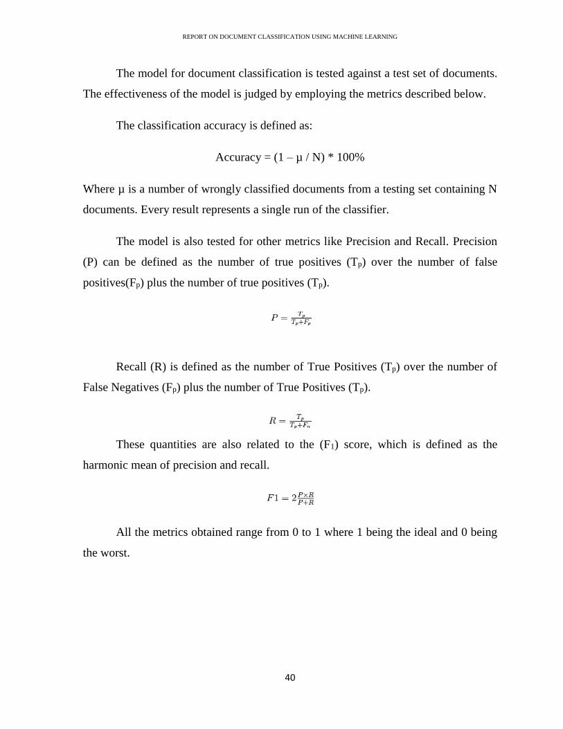
The model for document classification is tested against a test set of documents.

The effectiveness of the model is judged by employing the metrics described below.

The classification accuracy is defined as:

Accuracy = (1 – µ / N) * 100%

Where µ is a number of wrongly classified documents from a testing set containing N

documents. Every result represents a single run of the classifier.

The model is also tested for other metrics like Precision and Recall. Precision

(P) can be defined as the number of true positives (Tp) over the number of false

positives(Fp) plus the number of true positives (Tp).

Recall (R) is defined as the number of True Positives (Tp) over the number of

False Negatives (Fp) plus the number of True Positives (Tp).

These quantities are also related to the (F1) score, which is defined as the

harmonic mean of precision and recall.

All the metrics obtained range from 0 to 1 where 1 being the ideal and 0 being

the worst.


41

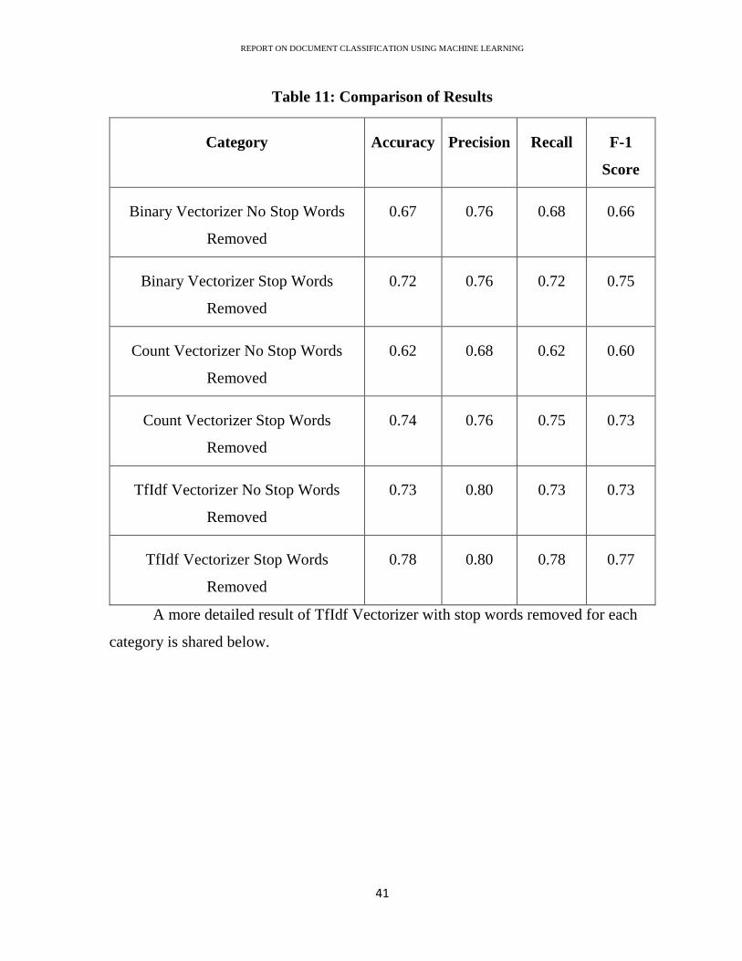
Table 11: Comparison of Results

Category Accuracy Precision Recall F-1

Score

Binary Vectorizer No Stop Words

Removed

0.67 0.76 0.68 0.66

Binary Vectorizer Stop Words

Removed

0.72 0.76 0.72 0.75

Count Vectorizer No Stop Words

Removed

0.62 0.68 0.62 0.60

Count Vectorizer Stop Words

Removed

0.74 0.76 0.75 0.73

TfIdf Vectorizer No Stop Words

Removed

0.73 0.80 0.73 0.73

TfIdf Vectorizer Stop Words

Removed

0.78 0.80 0.78 0.77

A more detailed result of TfIdf Vectorizer with stop words removed for each

category is shared below.


42

Table 12 : Classification report of Test Documents using TfIdf Vectorizer and

Naive Bayes Classifier

Detailed Classification report of other Vectorizers and their variants can be

found in the appendices. The first two appendices illustrate the classification report of


43

Binary vectorizer with and without stop words. The next two appendices describe the

classification report of Count vectorizer with and without stop words. Similarly the

last two appendices illustrate the classification report of TfIdf vectorizer with and

without stop words.

7 DISCUSSION OF RESULTS

As expected, TfIdf vectorizer outperformed the other two vectorizers, namely

the binary vectorizer and the count vectorizer. It gave 4% better accuracy than the count

vectorizer and 6% better accuracy than the binary vectorizer. It even obtained a better

Precision score of 0.80 compared to the count vectorizer and the binary vectorizer

which both obtained the best Precision score of 0.76. It outperformed the other two

vectorizers in Recall score as well getting a Recall score of 0.78 over 0.75 of the count

vectorizer and 0.72 of the binary vectorizer. Since F-1 Score is calculated based on

Precision and Recall, it naturally came better for TfIdf vectorizer. Numerically TfIdf

vectorizer achieved an F-1 score of 0.77 outperforming 0.75 of the binary vectorizer

and 0.73 of the count vectorizer.

As discussed in the Approach and Method section of the report, TfIdf vectorizer

performs better because it considers the distinguishability factor of each feature in

weighing compared to just the frequency of terms in count vectorizer or the mere

existence of a term in binary vectorizer. This makes the TfIdf vectorizer perform better

and represent the document in a more accurate way.

One interesting observation from the results is that if stop words in not removed

then, binary vectorizer does better than count vectorizer. Binary vectorizer got an

accuracy of 67% compared to the 62% of the count vectorizer. This is because a

document generally contains many stop words. Thus, if term frequency represents a

document, then the stop words are likely to become the most important feature of the

document. Since we know that stop words are never good discriminating criteria, it

results in misclassifications, leading to a drop in accuracy of predictions. On the other


44

hand, for binary vectorizer, stop words are registered as just 1, that is they exists in a

document. Thus, they do not overpower the significance of other discriminating words

that may be occurring in a document.

The TfIdf vectorizer performs well even when stop words are not removed. This

is because it considers the Idf (Inverse document frequency) value of each term as well

along with the frequency of the terms. Thus, even if we get the term frequency of some

stop word very high, the resulting TfIdf value of the term is decreased by the low Idf

value, since the TfIdf is a multiplication of Tf(Term frequency) and Idf (Inverse

document frequency).

The performance of TfIdf vectorizer is good across all categories except

categories of religion and politics. It is understandable since the two categories are a bit

correlated on their own and many documents of both the categories are broad enough

to have some correlation with the other category.

8 CONCLUSION AND FUTURE WORK

We would like to conclude that even though the binary vectorizer and the count

vectorizer works well, it is the TfIdf vectorizer that outperforms the two in terms of

both appropriate representations of documents and the classification results. Although

Count vectorizer performs well and better than binary vectorizer, it performs poorly

than binary vectorizer, if stop words are not removed.

In terms of categories, documents of most of the categories are classified with

precision, recall and F-1 score above 70%. The documents of the category of

religion.miscellaneous and the category of politics.miscellaneous were classified the

worst. The category of politics.mideast is classified the best with precision, recall and

an F-1 score of 0.90 each.


45

In order to test the classifier against the null hypothesis, one could perform

hypothesis testing using p-value. A p-value smaller than 0.05 indicates strong evidence

against null hypothesis and then the alternative hypothesis can be accepted.

We used just one algorithm, and that is Naïve Bayes for classification as the

main aim of our project work was to analyze the different types of feature representation

for documents. As a future work, We would suggest the researchers and students taking

the work forward to try and test the different feature representation schemes mentioned

with other machine learning algorithms like SVM, Neural Network, Expedition

maximization, Decision trees, etc.

We have not included in the report, another vectorizer that we tried and that is

Hashing Vectorizer. The hashing vectorizer although did not perform as well as TfIdf

vectorizer but was significantly faster than all the three vectorizer representation

mentioned in the report. It does not require the vocabulary to be present in memory all

the time, and thus it is space efficient as well. If the researcher wants to do document

classification in real time, We would suggest them to look into hashing vectorizer.

9 PROJECT SCHEDULE

The whole project work took around 3-4 months. Within this schedule, all the

tasks mentioned in the method and approach section of the report were carried out. A

very preliminary Naïve Bayes classifier was generated using Binary vectorizer by the

end of the fifth week. Rest of the tasks were completed in a span of 12 weeks after

which this report was written. A more detailed schedule is elaborated in the table below.

Table 13: Schedule employed for Project

EXPERIMENTS WEEK

DATA SET EXPLORATION 0-1


46

LOADING OF DATA SET 1-3

FEATURE REPRESENTATION USING BINARY

VECTORIZER

3-4

PRELIMINARY NAÏVE BAYES CLASSIFIER

WORKING

4-5

TESTING THE CLASSIFIER AND ADDING

LAPLACE SMOOTHING

5-7

REMOVAL OF HEADERS AND FOOTERS 7-8

REMOVAL OF STOP WORDS AND APPLICATION

OF STEMMING

8-9

FEATURE REPRESENTATION USING COUNT

VECTORIZER

9-10

FEATURE REPRESENTATION USING TFIDF

VECTORIZER

10-12

REPORT OF PROJECT WORK 12-14


47

REFERENCES

[1] Y. H. Li and A. K. Jain, “Classification of Text Documents,” [Online]. Available:

http://citeseerx.ist.psu.edu/viewdoc/download?doi=10.1.1.100.7400&rep=rep1&t

ype=pdf

[2] Thorsten Joachims, “Text Categorization with Support Vector Machines:

Learning with Many Relevant Features,” [Online]. Available:

http://www.cs.cornell.edu/people/tj/publications/joachims98a.pdf

[3] Konstantin Mertsalov and Michael McCreary, “Document Classification with

Support Vector Machines,” [Online]. Available:

http://www.rationalenterprise.com/assets/content/files/Classification_with_Suppo

rt_Vector_Machines.pdf

[4] Russell Power, Jay Chen, Trishank Karthik and Lakshminarayanan Subramanian,

“Document Classification for Focused Topics” [Online]. Available:

https://cs.nyu.edu/~jchen/publications/aaai4d-power.pdf

[5] Karel Fuka and Rudolf Hanka, “Feature Set Reduction for Document

Classification Problems” [Online] Available:

http://www.cs.cmu.edu/~mccallum/textbeyond/papers/fuka.pdf

[6] Myungsook Klassen and Nikhila Paturi, “Web document classification by

keywords using random forests,” [Online]. Available:

https://pdfs.semanticscholar.org/b489/157e3129d2b9a38a76c659a765be3ab8b2bc

.pdf

[7] A. Basu, C. Watters, and M. Shepherd, “Support Vector Machines for Text

Categorization,” [Online]. Available:

http://citeseerx.ist.psu.edu/viewdoc/download?doi=10.1.1.136.889&rep=rep1&ty

pe=pdf


48

[8] Quan Yuan, Gao Cong and Nadia M. Thalmann, “Enhancing Naive Bayes with

Various Smoothing Methods for Short Text Classification,” [Online]. Available:

http://www.ntu.edu.sg/home/gaocong/papers/wpp095-yuan.pdf

[9] “20 Newsgroup Data Set,” [Online]. Available:

http://qwone.com/~jason/20Newsgroups/

[10] Wikipedia: The free encyclopedia. (2004, July 22). FL: Wikimedia Foundation,

Inc. [Online]. Available: https://en.wikipedia.org/wiki/Document_classification

http://www.ntu.edu.sg/home/gaocong/papers/wpp095-yuan.pdf


49

APPENDICES

Appendix 1: Classification report of Binary Vectorizer with Stop words


50

Appendix 2: Classification report of Binary Vectorizer with Stop words removed


51

Appendix 3: Classification report of Count Vectorizer with Stop words


52

Appendix 4: Classification report of Count Vectorizer with Stop words removed


53

Appendix 5: Classification report of TfIdf Vectorizer with Stop words


54

Appendix 6: Classification report of TfIdf Vectorizer with Stop words removed