docking a metal nanoparticle to a protein surface by
TRANSCRIPT

Docking a Metal Nanoparticle to a Protein Surface
A Thesis submitted in partial fulfillment of the requirements for the degree of Master of Science at George Mason University
by
Jonathan Perkins Bachelor of Science
Randolph-Macon College, 2004
Director: Igor Griva, Associate Professor Department of Mathematical Sciences, George Mason University
Fall Semester 2014 George Mason University
Fairfax, VA

THIS WORK IS LICENSED UNDER A CREATIVE COMMONS
ATTRIBUTION-NODERIVS 3.0 UNPORTED LICENSE.
ii

DEDICATION
This is dedicated to my wonderful and supportive family.
iii

ACKNOWLEDGEMENTS
I would like to thank the many family members and friends who helped me edit and polish this work. I could not have done this without their continued dedication and patience. I would also like to thank my advisor Doctor Igor Griva who stuck with me despite the extended amount of time it took me to finish. I am thankful to my committee members Doctors Agnarsson, Goldin and Morris for their support and helpful suggestions. I also appreciate the resources and programming environments provided by George Mason University. I sincerely hope this model can be used to expand research and development in the field of mathematics and nanotechnology.
iv

TABLE OF CONTENTS
Page List of Tables ..................................................................................................................... vi
List of Figures ................................................................................................................... vii
List of Equations .............................................................................................................. viii
List of Abbreviations and Symbols.................................................................................... ix
Abstract ............................................................................................................................... x
Introduction......................................................................................................................... 1
Modeling Objectives........................................................................................................... 4
Mathematical Modeling Approach ..................................................................................... 5
The Method of Images for a Metal Sphere in a Field of Charges................................... 6
Expanding on the Method of Images .............................................................................. 9
Optimization Problem....................................................................................................... 12
AMPL Model Implementation.......................................................................................... 15
Sequential Quadratic Programming .............................................................................. 15
Visualization and Computational Tools............................................................................ 18
Setting up the Model with MATLAB ........................................................................... 19
Implementation Challenges .............................................................................................. 22
Numerical Results............................................................................................................. 24
Conclusion ........................................................................................................................ 30
Future Model Developments............................................................................................. 32
References......................................................................................................................... 34
v

LIST OF TABLES
Table Page Table 1 Optimal positions as N increases ......................................................................... 29
vi

LIST OF FIGURES
Figure Page Figure 1 Photosynthetic reaction center.............................................................................. 1 Figure 2 Electric field and surfaces of equipotential. ......................................................... 7 Figure 3 Spherical conductor in an electric field. ............................................................... 7 Figure 4 Geometry of the Method of Images...................................................................... 8 Figure 5 Expansion of the Method of Images................................................................... 11 Figure 6 Initial condition and solution visualization. ....................................................... 20 Figure 7 Initial conditions for data generation.................................................................. 24 Figure 8 SNOPT mean number of major iterations .......................................................... 25 Figure 9 SNOPT mean time to solve ................................................................................ 26 Figure 10 SNOPT number of minima found .................................................................... 27 Figure 11 SNOPT relative frequency of best solution...................................................... 28
vii

LIST OF EQUATIONS
Equation Page Equation 1 Potential Energy of a system of fixed and image charges.............................. 13 Equation 2 Applying the Method of Images and expanding in terms of x ....................... 13 Equation 3 Solving problem (P) finds the optimal position for a spherical electrode...... 14 Equation 4 First order optimality conditions for inequality constrained optimization..... 16 Equation 5 Inequality constrained QP sub-problem ......................................................... 16
viii

ix
LIST OF ABBREVIATIONS AND SYMBOLS
Central Processing Unit .................................................................................................CPU Gigabyte...........................................................................................................................GB Gigahertz........................................................................................................................GHz Nanometer........................................................................................................................ nm Photosynthetic Reaction Center.....................................................................................PRC Potential Energy................................................................................................................PE Quadratic Programming................................................................................................... QP Random Access Memory............................................................................................. RAM Sequential Quadratic Programming............................................................................... SQP

ABSTRACT
DOCKING A METAL NANOPARTICLE TO A PROTEIN SURFACE
Jonathan Perkins, M.S.
George Mason University, 2014
Thesis Director: Dr. Igor Griva
This thesis develops a mathematical and computational methodology for modeling
electrostatic interactions between a spherical electrode and the photosynthetic reaction
center (PRC) of the Rhodobacter Sphaeroides bacteria. A PRC is a protein-pigment
complex capable of photosynthetic reaction, converting light energy into chemical
energy. Recent studies suggest it is possible to use PRCs in the construction of next
generation photovoltaic devices. Modeling the electrostatic interactions between an
electrode and a PRC to find a position that optimizes electron transfer could improve
efficiency of technologies that use PRCs to generate electric current. The position is
found by minimizing the total electrostatic energy of the PRC-electrode complex. The
resulting nonlinear optimization problem can be solved reliably using a Sequential
Quadratic Programming algorithm. The model will provide the PRC-electrode structure
even as the problem grows in scope. It can be used as a tool for designing future
x

xi
technologies that take advantage of direct electron transfer between electrodes and
proteins.

INTRODUCTION
Over time, nature has evolved the photosynthetic reaction centers (PRC) to
convert light energy into chemical energy via photosynthesis. The PRC is one of most
advanced photovoltaic structures in nature [1]. Figure 1 illustrates the PRC of
Rhodobacter Sphaeroides. This structure is the protein-pigment complex that provides a
reliable way for the bacteria to generate energy via photosynthesis.
Figure 1 Photosynthetic reaction center
1

Understanding the principles of how a PRC behaves has led to the construction of
artificial photovoltaic and bio-photoelectronic structures [5][9]. Such structures can be
used in devices like solar panels that generate electricity from sunlight [1].
To operate successfully, these devices rely on the transfer of electrons between a
PRC and an electrode, in order to induce a current. Factors that facilitate the efficient
electron transfer between the PRC and the electrodes, such as positions and shapes, are
critical to the operation and overall efficiency of these devices. The position and shape of
the electrode is important because the distance between the PRC and electrode correlate
with the rate of electron transfer [6]. Calculating the best position for an electrode in
relationship to a protein surface is critical for achieving maximally efficient electron
transfer. These principles could apply to the design of photovoltaic nanodevices.
Determining the structural relationship between proteins and other objects (e.g.
smaller molecules) is generally referred to as protein docking. So far the scientific
community has been focused on finding a docked position of ligands which can be
viewed as "links" between the PRC and an electrode. Ligands are chemical or
biochemical structures that dock with proteins in specific ways. They can be used as
molecular wires that transfer electrons between an electrode and a protein.
Existing technologies use ligand gels attached to a conducting plate to facilitate
electron transfer between proteins and the conducting plate to induce current. The process
of docking ligands capitalizes on the lock-and-key mechanism based on spatial,
electrostatic, and vibrational constraints inherent to protein behavior.
2

However, using ligands can have drawbacks. In order to dock effectively, a ligand
must be highly specific to the protein with which it docks. The ligand must be specific
enough to be attracted to the protein in the desired manner without compromising the
protein's function. A ligand that is not specific enough for a purpose may cross react with
an inappropriate protein, not dock reliably with the protein of choice, or may denature the
protein in some way. The ligands themselves can also be rendered ineffective due to
environmental changes like temperature and pH. An example of the importance of ligand
specificity is Affinity Chromatography, where a ligand is used to immobilize a protein in
order to extract that protein from a solution [11].
The direct transfer of electrons between the protein and electrode is attractive
because it removes the need for ligands and can allow for more efficient electron transfer
[12]. A challenge associated with such an approach is placing the electrode in the best
position to facilitate efficient electron transfer with the PRC.
This thesis develops a mathematical methodology for modeling electrostatic
interactions between a spherical electrode, which can be produced using modern
technology, and a photosynthetic reaction center. A mathematical model is relatively
inexpensive and can provide useful insight for construction of devices that use a protein-
electrode complex. Developing a flexible model to find the optimal position for a metal
nanoelectrode relative to a specific protein can help further the development of
technologies such as bio-organic interfaces, biosensors, nanotechnology and photovoltaic
devices.
3

MODELING OBJECTIVES
A nanoelectrode of a specific shape and size could provide more efficient
functionality than a ligand would, i.e. facilitating even more efficient electron transfer.
Usually, the closer an electrode conforms to the surface of the protein, the more efficient
the electron transfer [2]. Choosing a size and shape of a nanoelectrode, finding its
docked position, then determining what kind of electron transfer it facilitates when
docked could be useful while attempting to develop better technologies. As a step
towards developing tools for studying these types of interactions, this thesis presents a
model that finds the docked position of a spherical nanoelectrode on a protein surface
that produces an efficient electron transfer between the protein and the electrode. Using
this model, a study of the interaction between a spherical electrode and a protein can be
done in an inexpensive and simple way.
According to the main principle of electrostatics, systems of charged particles
naturally arrange themselves to be at a minimum potential energy (PE) [8]. The proposed
model calculates the docked position of a spherical nanoelectrode by computing the
minimum PE. The next section describes this approach in more detail.
4

MATHEMATICAL MODELING APPROACH
Nanoscale modeling is challenging because structures such as a PRC and a metal
electrode have thousands of atoms that result in hundreds of thousands of interatomic
electrostatic interactions. As a first step towards modeling this complex interaction a
number of simplifications are made. First, assume that the protein is completely rigid. No
atoms within the protein are allowed to move. Such an assumption is justified because
the PRC used in the analysis is a relatively stable structure. Second, this model adopts
the hard-shell model for atoms within the protein, meaning that the electrode cannot
invade the radius of each atom. Such an assumption can be dropped in the future when a
dynamical model is considered. Third, a spherical shape of the nanoelectrode is used
without consideration of crystalline structure or any quantum effects of the metal
electrode. The nanoelectrode is large enough so that the model can use classical laws to
describe charges.
Lastly, assume that minimizing the total electrostatic potential energy of the
protein-electrode complex provides the docked position for the nanoelectrode on the
protein surface that facilitates the best electron transfer. The proposed methodology
should place the spherical electrode as close as possible to the location of the charge
separation in the PRC and therefore yield efficient electron transfer between the
photosynthetic reaction center and the electrode.
5

TheMethodofImagesforaMetalSphereinaFieldofCharges
Following the classical concept of induction, assume that some charge
distribution on the conducting sphere is induced by the charges in the PRC and can be
computed using the Method of Images [8][3]. Using the Method of Images, a conducting
sphere in a field of charges can be represented as a set of image charges. This re-
constructs the electric field generated by placing the spherical electrode near the protein.
A conducting sphere will always act as a surface of equipotential in an electric
field. This means the charges on the surface of the spherical electrode will arrange
themselves so that the potential is constant on the entire surface. If the potential were not
constant over the entire surface, then there would be an electric field inside the conductor
and the charges would re-distribute until the field became zero [3].
Consider the electric field generated by two point charges. The electric field has
contours, or surfaces of equipotential that are perpendicular to the electric field lines as in
Figure 2. Figure 2 is Figure 6-8 from Feynman's Lectures on Physics [3] illustrating an
electric field generated by two point charges, the field lines and surfaces of equipotential
A and B.
6

Figure 2 Electric field and surfaces of equipotential.
If a conducting sphere were placed to exactly fit surface A, shown in Figure 3,
then the electric field outside of surface A would be unchanged from the one generated
by a point charge. Figure 3 is figure 6-9 from Feynman's Lectures on Physics [3].
Figure 3 Spherical conductor in an electric field.
7

The electric field outside a conducting sphere can be re-created by substituting an
image charge to represent the equivalent surface of equipotential. The field generated by
a fixed charge q and a metal sphere, is re-created by placing an appropriate image charge:
at a suitable point some distance away from q. Figure 4 is Figure 6-11 from
Feynman's Lectures on Physics [3]. It Illustrates the Geometry for using the Method of
Images for a spherical conductor. Image charge q' is placed specifically so that all
positions P on the surface of the sphere will have equal potentials.
q
Figure 4 Geometry of the Method of Images
Assume a spherical surface of radius a that is centered some distance b away from
the position of the fixed charge q. Place an image charge of strength baqq at a
distance of ba2 from the center of the sphere. This causes a spherical surface (C) of
radius a, to be at zero potential.
To show this mathematically begin with the equation for the electric potential
at any point P due to any number of point charges , which is the sum of the eP iq
8

potentials from all charges [8]. This results in i i
iee r
qkP where is the ith charge, and
is the distance from point P to . There will be a potential of zero for each point P on
the surface at which . Substituting in the image charge
iq
ir iq
0eP q and the point charge q
from Figure 3 yields 01
r
q
r
q
2
kP ee. Divide out and subtract to get ek
21 r
q
r
q or
q
q
r
r
1
2 . Since baq q then
q
baq
r
r
1
2 or
b
a
r
r
1
2 . Therefore 1
2
r
rhas a
constant ratio of b
aand thus the surface has a zero potential when baqq .
For surfaces with a non-zero , as in an insulated conducting electrode, an
additional image charge q can be used to scale the surface to the proper PE value.
Finally, by setting an insulated or grounded conducting sphere can be accurately
modeled near charge q.
eP
ExpandingontheMethodofImages
This method can be expanded to create the same surface of equipotential in a field
of multiple charges. Each fixed charge will have an associated image charge iq iq and
each pair will create the same surface of radius a centered at the same location
when ii aqq ib , where is the distance from the fixed charge to the center of the
sphere.
ib
An electric field generated by placing a metal sphere in a field of known charges
and fixed locations given by a position vectors , can be re-created by placing n iq 3Rxi
9

image charges with charge values iii baqq at distances of iba 2 from the center of
the sphere for each fixed charge. Additionally, another image charge
N
iii baqq
1
is
placed at the center of the sphere to scale the surface to the proper PE.
Note that the sphere will naturally be drawn towards the fixed charges. The
charges representing the sphere have an overall attractive force with the fixed charges.
This means that the potential energy of the system of image and fixed charges will be at a
minimum when the sphere is at its closest to the protein surface.
However, the hard shell atom model used means the surface of the sphere should
not invade the space occupied by the protein. This results in constraints on the position of
the nanosphere that prevent overlapping of the nanosphere and protein. Each atom in the
protein is surrounded by a spherical region with a radius defined by the atomic size of the
atom, which is determined by the atom type. The metal nanosphere and atom's region
cannot overlap, so the distance between the sphere center and the atom center must be
larger than the sum of the radius of the metal sphere and the radius of the atom as seen in
Figure 5.
10

Figure 5 Expansion of the Method of Images
Figure 5 shows two atoms represented by charges and with radii and .
Their respective image charges
1q 2q 1r 2r
1q and 2q . To evaluate the total PE, the distances
must be calculated. ijD
11

OPTIMIZATION PROBLEM
The electrostatic interaction between a spherical electrode and a protein can be
modeled by accounting for the total potential energy (PE) for all the pairs of interactions
among all image charges (representing the spherical electrode) and the fixed charges (the
atoms within the protein). When computing the PE generated from a set of charges, a
point charge is placed in the electric field and is interacting with every other charge. The
PE is then calculated from the force exerted on the point charge by the other charges.
The same is true for a conductor in a field of charges; the electrode is interacting
with each fixed charge in the atom and so each fixed charge and the electrode contribute
to the PE of the whole system.
Earlier it was shown that the Method of Images can be used to re-create the
electric field outside the electrode by using a set of image charges. The set of image
charges can be used to compute the PE between the electrode and protein.
In this approach the PE is completely defined by the interactions between image
charges and fixed charges only, as it would between the electrode and each fixed charge.
The interactions among image charges do not contribute to the overall PE of the system
because they are not real, they only represent the electric field outside the spherical
electrode. The interactions among fixed charges also do not contribute to the PE
12

calculation simply because their position and values are fixed; hence the PE among those
charges is constant.
Equation 1 shows the PE of the electrode-sphere system written as a function
: of the sphere's center position )(xPE RR 3 ),,( zyxx
N
i i
iN
i
N
j ij
ji
b
D
qqxPE
11 1
)(
Equation 1 Potential Energy of a system of fixed and image charges
where is the distance between ith image charge and jth fixed charge, is the charge
value for the jth fixed charge,
ijD jq
iq is the image charge value for the ith fixed charge.
The distance jiij xxD is the magnitude of the difference between vectors ix
and . The vector is the position of the jth fixed charge andjx jx ix is the position of the ith
image charge. In other terms 22)( iii baxxxx where ii xxb is the distance
between x and the ith fixed charge . The ith image charge value is ix iii baqq . So,
using this notation, Equation 2 shows the PE of the sphere-protein system written as a
function of the sphere's center position x:
N
i i
iN
j j
j
N
i
N
j
j
i
i
ji
i
xx
q
xx
aq
xxx
axxx
qxx
aq
xPE111 1
2
2
)(
)(
Equation 2 Applying the Method of Images and expanding in terms of x
This function is to be minimized subject to constraints on the position of the
sphere. These constraints result from the fact that the atoms and the electrode cannot
13

overlap. For each atom, the distance between the sphere's center and the center of the
atom must be greater than or equal to the sum of their radii. These constraints can be
expressed by where a is the radius of the sphere and is the radius of the ith
atom. Expressed as a vector function, is composed of N constraints:
arb ii ir
NRRxh 3:)(
0 })({)( arxxxhxh iii for i = 1...N
Finally, this forms an inequality constrained non-linear optimization problem,
problem (P) shown in Equation 3. Solving problem (P) finds the optimal position for a
spherical electrode relative to a protein whose atomic structure is defined by the set of
atoms.
Minimize over x:
N
i i
iN
i
N
j ij
ji
b
D
qqxPE
11 1
)( (P)
subject to 0 })({)( arxxxhxh iii
Equation 3 Solving problem (P) finds the optimal position for a spherical electrode
One approach to solving this problem is to use A Modeling Language for
Mathematical Programming (AMPL) to formulate the problem so that solvers, which
implement different optimization techniques, can be applied to compute a solution.
14

AMPL MODEL IMPLEMENTATION
A Modeling Language for Mathematical Programming (AMPL) is a generic
scripting programming language that can be used to formulate optimization problems
[13]. It provides a generic setting for the evaluation of optimization problems while
allowing external solvers to perform the calculations. Linear and non-linear optimization
problems are best solved by using the appropriate algorithm. One of the main attractive
AMPL features is that it automatically provides all the derivatives for the objective
function and constraints required for the optimization method to solve the problem.
Different AMPL solvers apply different techniques for evaluating each
optimization task. Some solvers perform better when many constraints are used, some
perform better when many independent variables are used. Problem (P) is a large-scale
inequality constrained optimization problem with non-linear objective function with three
variables and N non-linear constraints. SNOPT is a solver that is well suited for solving
this problem. SNOPT implements a sequential quadratic programming (SQP) method [4].
SequentialQuadraticProgramming
Sequential Quadratic Programming (SQP) is a method for solving constrained
nonlinear optimization problems [7]. SQP begins its process by reframing the problem in
terms of the Lagrangian function , where x is the original vector
of independent variables, and λ is the vector of Lagrange multipliers, one for each
)()(),( xhxPExL T
15

constraint. The Lagrangian function is formed by combining the objective function
: with its constraints using Lagrange multipliers . )(xPE RR 3 NRRxh 3:)(
)(
)(
)()(
xh
xh
xhxPET
T
NR
The solution to problem (P) must satisfy the first order optimality conditions
indicated in Equation 4[7].
0
0
0
0
Lx
Equation 4 First order optimality conditions for inequality constrained optimization
Given an initial guess ),( 00 x SQP solves problem (P) iteratively through the
sequence of quadratic sub-problems. The QP sub-problem shown in Equation 5
minimizes the quadratic approximation to the Lagrangian subject to linearized constraints
from the original problem about some current guess ), iix( . The solution to the QP sub-
problem is an update vector ( ), x where is the solution to the QP problem andx is
the Lagrange multipliers for the QP sub-problem.
Minimize over : x ))()((),(2iixx
T xxLx )21 iiT
iT xhxPEx (
subject to 0 ()( i xhxxh )i
Equation 5 Inequality constrained QP sub-problem
Where and
N
ihiPE HxHxL
1
)(),( )(xhT xx2
)x )(xHih
)(),( xPExL x
)(xhi
xi
)(
)(xHPE is the Hessian matrix of and is the Hessian of each constraint
function . The Hessian matrix is the Jacobian matrix of the gradient of a function. It
is the matrix of second-order partial differentials.
(PE
16

23
2
23
2
13
232
2
22
2
12
231
2
21
2
21
2
)()()(
)()()(
)()()(
)(
x
xPE
xx
xPE
xx
xPExx
xPE
x
xPE
xx
xPExx
xPE
xx
xPE
x
xPE
xH PE
23
2
23
2
13
232
2
22
2
12
231
2
21
2
21
2
)()()(
)()()(
)()()(
)(
x
xh
xx
xh
xx
xhxx
xh
x
xh
xx
xhxx
xh
xx
xh
x
xh
xH
iii
iii
iii
hi
For each guess ),( iix , an update vector is calculated ),( iix , then a next
guess is found as ),,( 1 iiiii xx ()1i x , the QP sub-problem is formed again and
the process is repeated. The sequence ),( iix eventually converges to a point satisfying
the first order optimality conditions and thus is a solution of problem (P)[7]. Each
iteration resulting in a new guess is a major iteration.
The QP sub-problem can be solved using different techniques such as interior-
point or simplex methods. Most techniques for solving the quadratic sub-problems are
iterative themselves and so those iterations are called minor iterations of the SQP method.
17

VISUALIZATION AND COMPUTATIONAL TOOLS
Optimization problem (P) is implemented as an AMPL model. The AMPL model
relies on initial conditions and data parameters to be set up prior to running AMPL
model. These parameters are the atom positions, charges, and sizes. The initial conditions
are a selected position and radius for the electrode. This research developed a set of
MATLAB® scripts to automatically create input files to the AMPL model, run the
AMPL model, and collect output data.
MATLAB version R2007b was selected because it has the ability to 1) read and
write data files, 2) create re-usable functions and scripts, 3) execute command line AMPL
models within a script, 4) create plots, and 5) provide computational support for post-
processing of the results from the AMPL model. This work can be easily expanded with
new MATLAB scripts and functions.
The visualization tool selected for this project is an academic version of
Accelrys® Discovery Studio® Visualizer (DSV). It is used to display the starting
conditions and solutions. DSV supports many different molecular formats, in this case a
mol2 file format was used. This is a file format developed and maintained by Tripos®.
These tools are used to visualize molecular structures in a 3D environment and are a
significant improvement over the visualizations of the same data within MATLAB.
18

SettinguptheModelwithMATLAB
In order to execute the AMPL model a process for setting up the input to AMPL
was developed using MATLAB scripts. The MATLAB scripts are generic enough to be
used on any mol2 file that contains the atomic structure of a protein. MATLAB is also
used to execute the AMPL model, parse output, and translate the solution back into a
mol2 data file in order to visualize the results. MATLAB scripts can also sort and scope
the data that the AMPL model then uses. The process is as follows:
1) Specify a mol2 file of protein data, a scope (N), position (xyz) and radius (r)
for the spherical electrode.
Write the initial conditions mol2 file for visualization
2) Parse the positions of the protein's atoms from the mol2 file.
3) Sort the protein's atoms from nearest to furthest from the electrode's position.
4) Select the N nearest to the given electrode position.
5) Determine each atom's radius.
6) Write the AMPL parameter and initial condition files.
7) Run the AMPL model.
8) Read the AMPL and SNOPT output files.
Write the solution to a mol2 file for visualization.
The atom positions, types, and charge values were extracted from the mol2 file.
However, the mol2 file does not contain the atomic size of each atom. Atomic size data
was obtained from crystallographic data [10]. In a hard-shell atom model the atomic size
is used as the radius of the atom. In order to pair the atom data from the mol2 file with
19

the appropriate atomic size, a lookup table that maps each atom type with it's atomic size
was generated.
Figure 6 shows screen captures from Discovery Studio 3.1 Visualizer displaying
the initial conditions (left) and solution (right) from executing the AMPL model.
Figure 6 Initial condition and solution visualization.
Once the fixed atoms are sorted from nearest to furthest, the N nearest atoms' data
is written to an AMPL parameter file, along with other constants N and the radius of the
sphere. These are used in the execution of the AMPL model.
In this implementation, there are three AMPL files, the parameter file containing
the constants, the initial condition file containing the starting position for the sphere, and
the AMPL model file containing the equations and solver options. The AMPL model file
20

is independent of any data so that the MATLAB scripts can be used to generate different
parameter files without modifying the AMPL model file.
21

IMPLEMENTATION CHALLENGES
Implementing the mathematical model in AMPL has some challenges. As stated
above, the data in the mol2 file needed to be preprocessed into a format that AMPL can
use. This leads to the first challenge: automatic parsing of the data file to collect all the
required information about PRC structure. The second challenge was hardware
constraints, which limited the size of the problem that could be solved by the AMPL
model.
The AMPL model requires the position, charge and radius of each atom within the
protein. The results in the next section were produced from using a mol2 file generated
by SYBYL software (a Tripos product). Collecting the atomic radii of each atom type
and relating it to the data in the Tripos file was done with another MATLAB script to pull
in all appropriate data for the model.
Once all data is collected and processed into a data file for AMPL, the AMPL
model can be executed, handing the proper information to the SNOPT solver to find a
solution. This leads to the largest roadblock to this implementation: available memory.
The model was executed on available hardware that lacked sufficient memory capacity to
support the SQP implementation in SNOPT. Through a number of trial and error
attempts, a maximum number of about 1200 atoms could be sent to the SNOPT solver
before an out-of-memory error was reached. This limitation depends on the computer
22

hardware that is executing the model. The data presented below was generated on a
Windows(TM) 7 64-bit platform with an Intel(R) Core(TM) i7 CPU @1.73GHz with
6GB of RAM.
To alleviate this issue the problem can be down-scoped to only the N nearest
atoms to the starting location. This is a necessary concession and is acceptable as the
nearest atoms are those that would have the most impact on the PE of the entire system.
Additionally, only those atoms nearest the starting location would be restricting the
position of the electrode as it docked to the surface of the protein. Therefore, yet another
MATLAB tool will read in the protein data, sort the atoms from nearest to furthest given
some starting location, and print the N nearest atom data to the AMPL data file.
The implementation of this model was also challenging. The data necessary for
the AMPL model needed to be collected from multiple sources. The amount of memory
needed to store the structures SNOPT uses in the optimization computations is
prohibitive for solving the problem for the entire protein. Scoping down the problem has
allowed a proof-of-concept for this model, however it does limit the accuracy of results
and is a consideration for future work.
23

NUMERICAL RESULTS
This section presents data indicating the performance and reliability of the model
implementation as the scope of the problem increases. To begin, an initial position is
selected in a region where the metal nanosphere is sought to be docked and a spherical
electrode with a radius of 1 nm is selected, giving us a starting situation seen in Figure 7.
Figure 7 Initial conditions for data generation
24

To vary the scope of the problem, a set of N atoms were taken into account when
creating the input data for the fixed charges in the AMPL model. N ranged from 50 to
1200 in increments of 50. To evaluate the model's reliability for each value of N, a
spherical grid with a radius of .5 nm was created about point S. The grid was comprised
of 130 evenly spaced starting locations, the intersection points of 8 parallels and 16
meridians plus the two poles. The model was executed using each grid point as a starting
location. For each execution, the resulting position, the PE(x) at that position, the number
of major iterations and the execution time of the solver were recorded. Finally, For each
value of N, the mean number of iterations, the mean execution time, the total number of
unique solutions, and the frequency of the best solution were calculated.
Figure 8 SNOPT mean number of major iterations
25
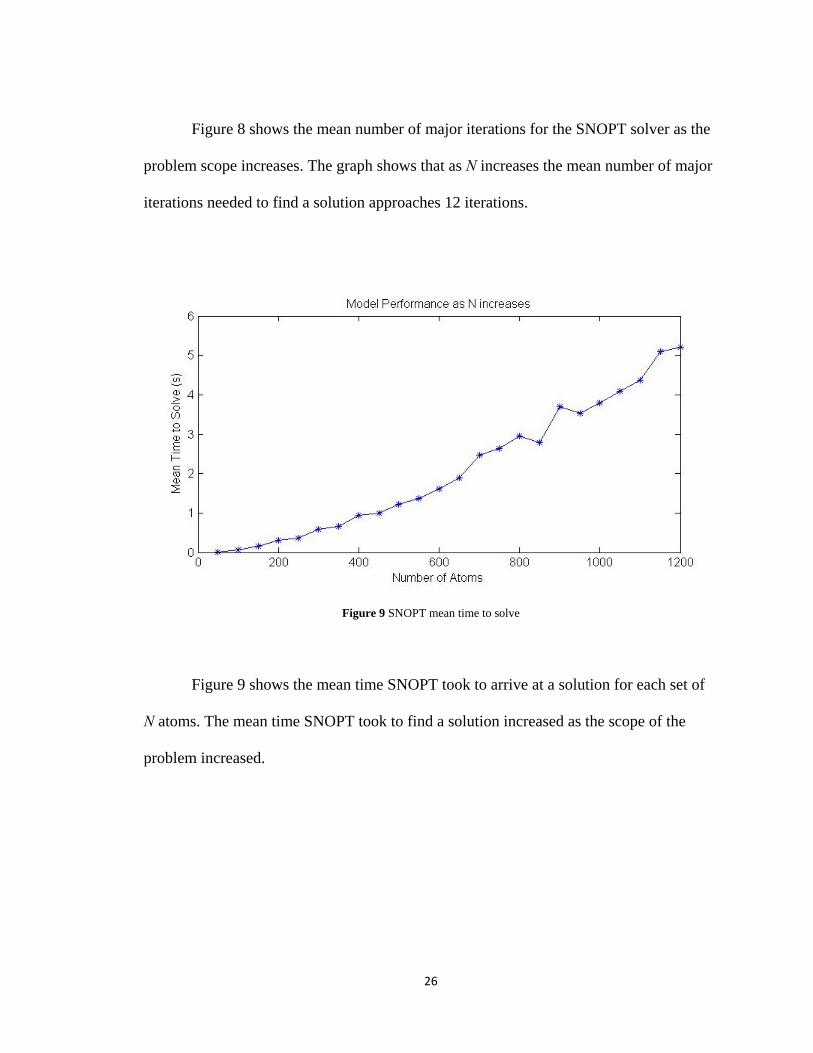
Figure 8 shows the mean number of major iterations for the SNOPT solver as the
problem scope increases. The graph shows that as N increases the mean number of major
iterations needed to find a solution approaches 12 iterations.
Figure 9 SNOPT mean time to solve
Figure 9 shows the mean time SNOPT took to arrive at a solution for each set of
N atoms. The mean time SNOPT took to find a solution increased as the scope of the
problem increased.
26

Figure 10 SNOPT number of minima found
Sometimes SNOPT found different solutions corresponding to different starting
positions for a given value of N. Figure 10 shows the number of distinct solutions with a
relative difference of greater than 1%. The worst case, with N=400, shows that the
number of different minimums found for a given spherical grid was seven(7). However,
for N=500, 850, 900, and 950, only one solution was found. This data indicates that the
tendency to find more than one solution does not seem to correlate with the size of the
problem.
27

Figure 11 SNOPT relative frequency of best solution
Figure 11 shows the relative frequency of finding the best solution for each N.
The relative frequency of finding the best solution also shows no trend with size of the
problem.
Table 1 shows the coordinates of the best solution for each N. For reference, the
initial positions of the sphere centers were located about (-10, 135, 57). The solution
positions are numbered to indicate optimal positions that were repeated as the complexity
increased. It is important to note that after N reaches a certain value, position 3 was
repeatedly found to be the best position more than any other position. This may mean
that there is some useful value of N beyond which there is no change in the optimal
position. Thus, it may be possible to find the optimal position without using the entire
protein.
28

Table 1 Optimal positions as N increases Optimal Position Coordinates Position
# N x y z 50 -7.5404 114.8660 44.7493 1 100 -7.5404 114.8660 44.7493 1 150 -7.5404 114.8660 44.7493 1 200 -0.6612 113.5543 41.6490 2 250 -0.6612 113.5543 41.6490 2 300 -0.6612 113.5543 41.6490 2 350 2.9850 111.5108 45.8645 3 400 -0.0314 113.3758 40.6087 4 450 2.9850 111.5108 45.8645 3 500 2.9850 111.5108 45.8645 3 550 2.9850 111.5108 45.8645 3 600 2.9850 111.5108 45.8645 3 650 -0.0314 113.3758 40.6087 4 700 2.9850 111.5108 45.8645 3 750 -0.0314 113.3758 40.6087 4 800 2.9850 111.5108 45.8645 3 850 2.9850 111.5108 45.8645 3 900 2.9850 111.5108 45.8645 3 950 2.9850 111.5108 45.8645 3 1000 2.9850 111.5108 45.8645 3 1050 2.9850 111.5108 45.8645 3 1100 2.9850 111.5108 45.8645 3 1150 2.9850 111.5108 45.8645 3 1200 2.9850 111.5108 45.8645 3
Numerical solvers that can be used with AMPL can sometimes have difficulty
finding a solution. Solvers can reach an iteration limit or arrive at some infeasible
solution or any of a number of error conditions. SNOPT did not demonstrate any issue
with finding a solution for problem (P), every one of the executions arrived at a solution.
29

CONCLUSION
This thesis has developed the methodology for finding the docking position of a
spherical metal nanoelectrode on the surface of a protein. A mathematical model based
on the electrostatic interactions between the atoms in the protein and a metal
nanoelectrode was developed. An implementation of the model using the AMPL
modeling language was presented and shown to reliably provide an optimal position of
the metal nanoelectrode. Our results demonstrate that the developed methodology can be
reliably used for preliminary estimation of the position of the nanoelectrode on the
protein surface.
This work was motivated by the desire to improve efficiency of the photovoltaic
devices with bio-organic interfaces. Such devices rely on efficient electron transfer
between proteins and nanoelectodes in order to produce electrical current. Estimation of
the position of the nanoelectrode on the protein surface helps modeling functionality of
the devices.
One of the key contributions of this thesis is developing the a mathematical model
of the electrostatic interaction between a spherical metal nanoelectrode and a protein.
Starting with a few simplifications and by applying the Method of Images, this thesis
shows that the position of the metal nanosphere can be computed by solving a nonlinear
30

optimization problem. The developed optimization problem was solved using the method
of Sequential Quadratic Programming, as implemented in the nonlinear programming
package SNOPT.
AMPL is an effective modeling environment for formulating the optimization
problem, giving access to many different solvers, employing many different techniques.
SNOPT is one solver designed for large scale nonlinear optimization problems and
performs reliably in this case. Using AMPL to formulate and SNOPT to solve, a solution
was found 100% of the time and seemed to converge to a relatively low number of
iterations even as the problem grew in scope.
There were several challenges in implementing the model with these tools.
Collecting all of the data is difficult. Atomic sizes are missing from the popular mol2 file
format and so external sources of that data must be relied upon and associated with the
proper atom types. Hardware limitations posed another challenge with this
implementation. The available memory allowed only a small portion of the protein to be
taken into account. A maximum of 1200 of the 14935 atoms (8.3%) in the protein were
used when executing the model. More than 1200 would cause an out-of-memory error.
In summary, the developed methodology although based on a number of
simplifications can be used to estimate a position of the sphere. It is a first step towards a
more complex model. A model implementation is presented and evaluated along with a
discussion of implementation and visualization tools. In the next section we discuss
some future directions for further developing the model.
31

FUTURE MODEL DEVELOPMENTS
Future developments can be made to improve the accuracy of the model. A next
step could be to introduce molecular flexibility to the model that accounts for
deformations of the protein. The protein discussed here is stable and assumed to be rigid,
nevertheless when an electrode comes in contact with a protein, the latter may change
shape a little. This would change the electric field around the protein, and may have an
effect on the docked position of an electrode. A dynamic model for electrode-protein
docking could be used to study the process of formation of the electrode-protein complex
in real time. Improving the model to account the effect of the deformation of the protein
could be valuable.
Another improvement would be to expand the model to include a better model of
an atom size. A more accurate interpretation of how the atoms interact when they are
close would be an additional step for the model development. This model assumes a hard
shell model of each atom, providing a convenient way to describe the constraints for the
developed optimization problem. The constraints impose a distance restriction between
the electrode and each atom in the protein. With a better model of how atoms interact at
these distances the constraints of the optimization problem could be relaxed to achieve
better accuracy.
32

Relaxing assumptions made in building this model, such as a rigid protein and
hard-shell atoms, would lead to an improvement of the objective function. It would no
longer be a calculation of just the PE, but a combination of other interactions at play. All
of these future developments would make the model more accurate but would increase
the complexity that may require significant changes in the implementation.
33

REFERENCES
1. Blankenship, R. E., D. M. Tiede, J. Barber, G. W. Brudvig, G. Fleming, M. Ghirardi, M. R. Gunner, W. Junge, D. M. Kramer, A. Melis, T. A. Moore, C. C. Moser, D. G. Nocera, A. J. Nozik, D. R. Ort, W. W. Parson, R. C. Prince, and R. T. Sayre. "Comparing Photosynthetic and Photovoltaic Efficiencies and Recognizing the Potential for Improvement." Science 332.6031 (2011): 805-09. Web.
2. Boxer, S. "Mechanisms Of Long-Distance Electron Transfer In Proteins: Lessons
From Photosynthetic Reaction Centers." Annual Review of Biophysics and Biomolecular Structure 19.1 (1990): 267-99. Print.
3. Feynman, Richard P., Robert B. Leighton, Matthew Sands, and S. B. Treiman. "The
Feynman Lectures on Physics." Physics Today 17.8 (1964): 45. Print. 4. Gill, Philip E., Walter Murray, and Michael A. Saunders. "SNOPT: An SQP
Algorithm for Large-Scale Constrained Optimization." SIAM Review 47.1 (2005): 99. Web.
5. Gorton, L. Biosensors and Modern Biospecific Analytical Techniques. Amsterdam:
Elsevier, 2005. Print. 6. Griva, Igor, Joel M. Schnur, and Nikolai Lebedev. "The Role of Electrode Curvature
in Controlling Electron Transfer between the Photosynthetic Reaction Center Protein and Gold Nanoelectrodes." ChemPhysChem 11.17 (2010): 3589-591. Print.
7. Heath, Michael T. Scientific Computing: An Introductory Survey. Boston: McGraw-
Hill, 2002. Print. 8. Serway, Raymond A., and John W. Jewett. Physics for Scientists and Engineers.
Pacific Grove, CA: Brooks/Cole, 2003. Print. 9. Takshi, Arash, John D.w. Madden, Ali Mahmoudzadeh, Rafael Saer, and J. Thomas
Beatty. "A Photovoltaic Device Using an Electrolyte Containing Photosynthetic Reaction Centers." Energies 3.11 (2010): 1721-727. Web.
34

10. University of California, Davis, comp. Covalent Radii. Chemwiki. University of California, Davis. Web. 16 Mar. 2014. <http://chemwiki.ucdavis.edu/Reference/Reference_Tables/Atomic_and_Molecular_Properties/Covalent_Radii>.
11. Voet, Donald, Judith G. Voet, and Charlotte W. Pratt. Fundamentals of Biochemistry.
New York: Wiley, 1999. Print. 12. Zhang, Wenjun, and Genxi Li. "Third-Generation Biosensors Based on the Direct
Electron Transfer of Proteins." Analytical Sciences 20.4 (2004): 603-09. Print. 13. Fourer, Robert, David M. Gay, and Brian W. Kernighan. AMPL: A Modeling
Language for Mathematical Programming. Pacific Grove, CA: Thomson/Brooks/Cole, 2003. Print.
35

36
BIOGRAPHY
Jonathan Perkins graduated from Robinson Secondary School, Fairfax, Virginia in 2000. He received his Bachelor of Science from Randolph-Macon College in 2004 with a double major in Mathematics and Computer Science. Since 2003 he has been employed as a Scientist at the Naval Surface Warfare Center in Dahlgren, Virginia in the Strategic and Weapon Control Systems Department.