Do stem form differences mask responses to silvicultural

treatment?

Doug Maguire

Department of Forest Science

Oregon State University

Typical responses monitored during silvicultural trials

-Dbh

-Height

-Height to crown base?

-Upper stem diameters??

-Branch diameters??

Monitor Dbh and Ht (perhaps crown size), but do regional or subregional volume/taper equations adequately estimate tree volumes?

How would you test statistically for silvicultural treatment effects on stem form?

Lennette thesis – Effects of stand density regime on stem form in larch

Garber thesis – Effects of initial spacing and species mix on tree and stand productivity

Scott Ketchum, Robin Rose – Does relative stem profile respond to early control of competing vegetation?

Mark Gourley et al. – Are Swiss needle cast and/or nutrient amendments changing stem form in Douglas-fir?

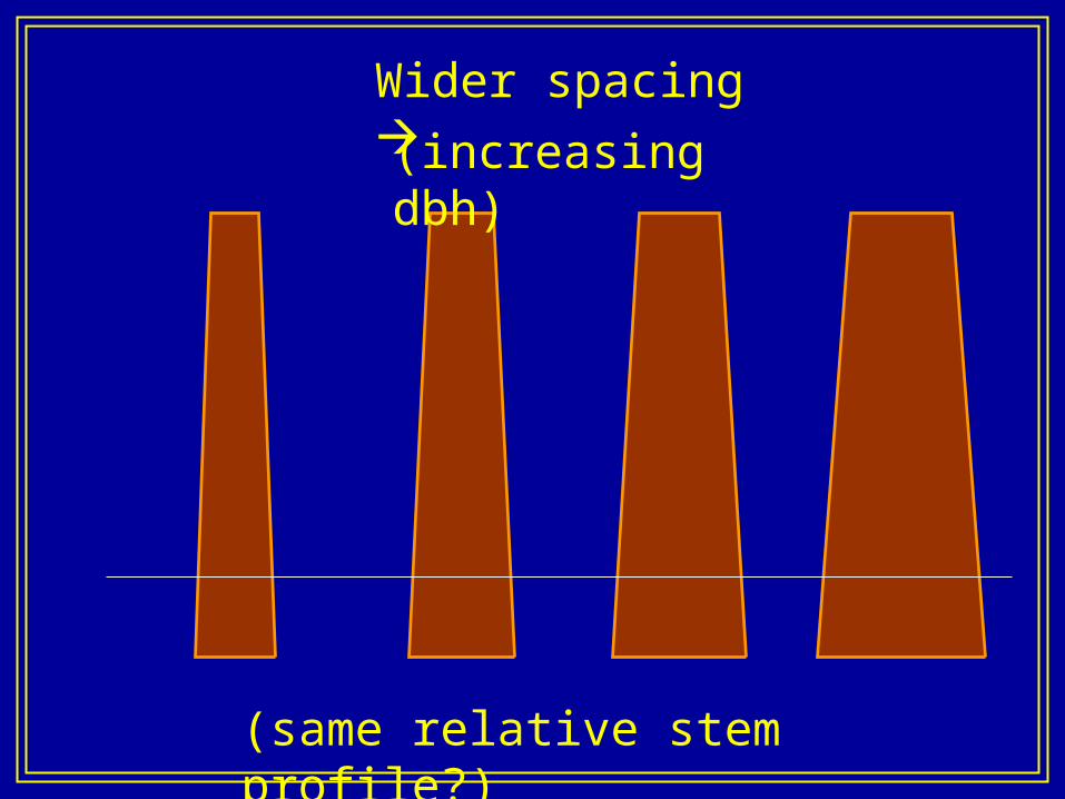
Wider spacing

(same relative stem profile?)

(increasing dbh)

Wider spacing

Larger crowns

(length and width)

Change in relative stem profile?

Influence on distribution of bole increment

Are any responses in stem form accounted for by monitoring treatment

effects on crown size (length)?

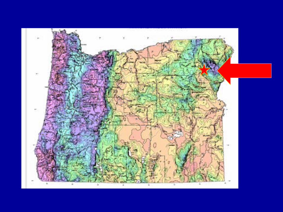
Andy Lennette. 1999. Twenty-five-year response of Larix occidentalis stem form to five stand density regimes in the Blue Mountains of eastern Oregon. M.S. Thesis, Oregon State University

Lexen (1943): bole surface area as measure of growing stock

(Approximation of cambial surface area on which wood accrues)

=>Measurement of bole surface area to regulate stocking

Catherine Creek Levels-of-growing-stock study

Stocking regulated by bole surface area

=>Accomplished with Barr and Stroud optical dendrometer

=>Many upper stem measurements over time

Growing stock levels

1: 5,000 ft2/ac

2: 10,000 ft2/ac

3: 15,000 ft2/ac

4: 20,000 ft2/ac

5: 25,000 ft2/ac

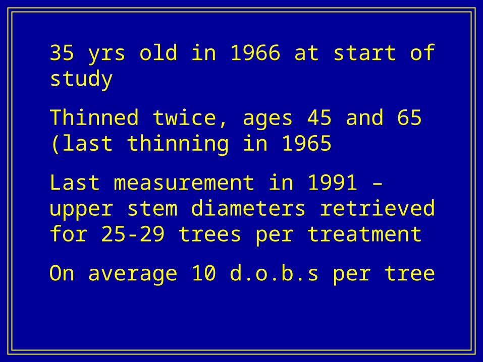
35 yrs old in 1966 at start of study

Thinned twice, ages 45 and 65 (last thinning in 1965

Last measurement in 1991 – upper stem diameters retrieved for 25-29 trees per treatment

On average 10 d.o.b.s per tree

GSL Dbh (in) Ht (ft)

I 16.183.6

II 12.274.1

III 11.473.7

IV 10.772.6

V 9.574.8

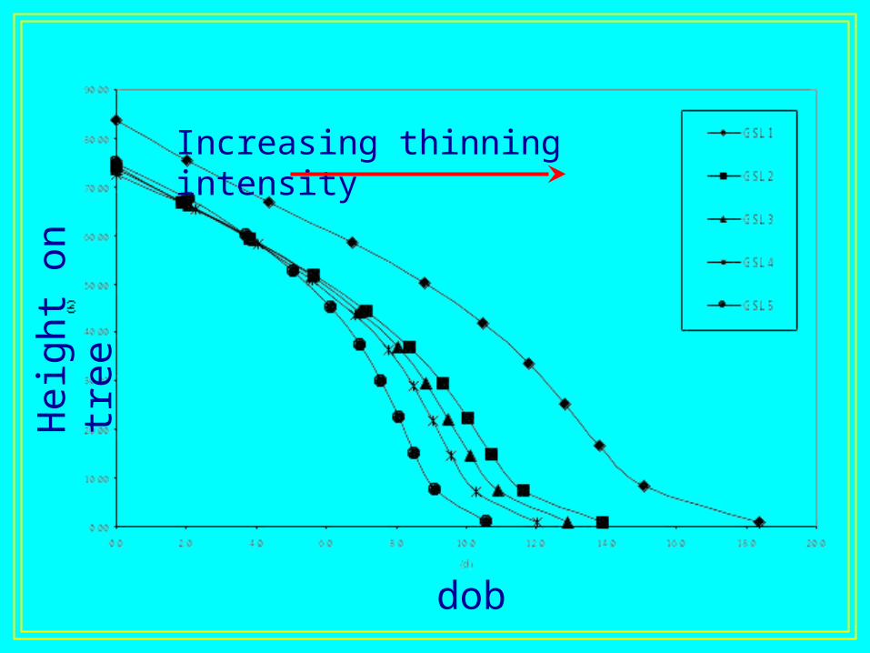
Increasing thinning intensity

dob

Hei

ght o

n tr

ee

35

40

45

50

55

60

65

70

75

0 1 2 3 4 5 6

GSL

Cro

wn

Rat

io(%

)C

row

n ra

tio

Increasing thinning intensity

Analysis:

Kozak variable exponent model

Dob/DBH = XC

where X = [1-(h/H)0.5] / [1-(4.5/H)0.5]

C = a1sin-1(h/H) + a2(h/H)2

Fitted to each individual tree, then SUR for

a1 = f( GSL or tree attributes (eD/H) )

a2 = g( GSL or tree attributes (CR) )

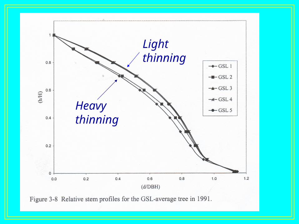
Increasing thinning intensity

dob

Hei

ght o

n tr

ee

Heavy thinning

Light thinning

Light thinning

Heavy thinning

Light thinning

Heavy thinning

Conclusions:

Relative stem profile was significantly different between the 2 most intensive thinning treatments, and these 2 were significantly different than the 3 least intensive thinnings

There was no marginal effect of treatment beyond its effect on D/H and crown ratio

Production analysis requires development of taper/volume functions

(without attempt at explicit test of treatment effects on stem profile)

Sean Garber. 2002. Crown structure, stand dynamics, and production ecology of two species mixtures in the central Oregon Cascades. M.S. Thesis, Oregon State University

Ponderosa pine/lodgepole pine mixed species spacing trial, planted in 1967

Grand fir/ponderosa pine mixed species spacing trial, planted in 1974

Both sampled in fall 2001 (34 and 27 yrs old, respectively)

Upper stem measurements from trees felled outside of permanent spacing trials

Analysis based on Kozak variable exponent model:

Dob/DBH = XC

where X = [1-(h/H)0.5] / [1-(4.5/H)0.5]

C = f(h, H, and D)

Objective was NOT to test for spacing and species effects on stem form, but rather on relative productivity. BUT needed a reliable volume or taper function for the site.

Rather than two-stage approach, can a mixed-effects model be applied ?

Is a random tree effect sufficient to eliminate autocorrelation among observations within a tree?

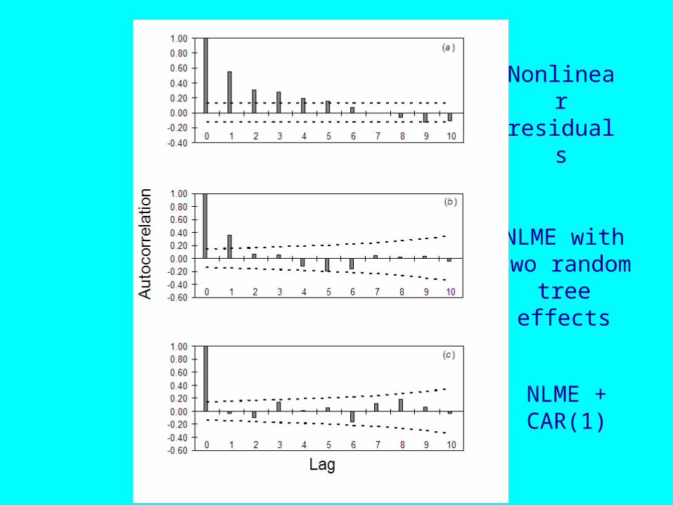
Nonlinear residuals

NLME with two random tree effects

NLME + CAR(1)

Grand fir

Ponderosa pine

Lodgepole pine

Ponderosa pine

Subtle spacing effects on relative stem profile

(but estimated adequately from D/H)

Average tree in each spacing

Spacing effect was not tested explicitly in taper model since trees were felled off the plots

Instead profiles were plotted for the tree of average dbh and height within each spacing-species combination

Effect of species composition was even more subtle

Conclusions:

Random tree effect dramatically reduced the order of autocorrelation, but did not eliminate it.

A first-order continuous autoregressive error process eliminated the remaining autocorrelation.

Conclusions (continued):

The taper functions had <3% bias in almost all cases.

Regional volume equations (Cochran 1985) differed from the taper equation estimates by 20-30% for grand fir, 20-60% for lodgpole pine, and 2-10% for ponderosa pine.

Rose, Ketchum, & Hanson. 1999. Three-year survival and growth of Douglas-fir seedlings under various vegetation-free regimes. Forest Science 45:117-126.

8 treatments, 3 reps/trt @ each of 2 sites

Area of herbaceous and woody control (1st two growing seasons):

0, 4, 16, 36, 64, 100 ft2

+ 100 ft2 woody only

+ 100 ft2 herbaceous only

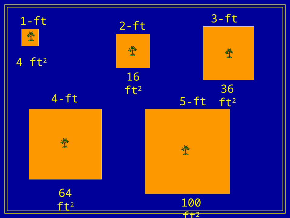
1-ft 2-ft3-ft

4-ft 5-ft

4 ft2

64 ft2

16 ft2

36 ft2

100 ft2

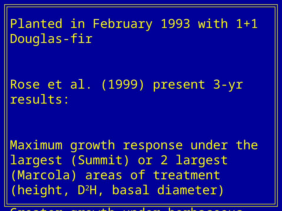
Planted in February 1993 with 1+1 Douglas-fir

Rose et al. (1999) present 3-yr results:

Maximum growth response under the largest (Summit) or 2 largest (Marcola) areas of treatment (height, D2H, basal diameter)

Greater growth under herbaceous only, not under woody only, relative to controls

Winter 2001-2002, stem d.o.b. measurements

Does the intensity of early weed control affect stem profile beyond the effect on diameter and height?

Do existing volume equations accurately predict stem volume of weeded plantations?

Difference = observed - predicted

0

5

10

15

20

25

30

-0.5 -0.4 -0.3 -0.2 -0.1 0 0.1 0.2 0.3

Difference (in)

Hei

ght (

ft)

Marcola

Summit

Difference = observed - predictedSummit and Marcola averaged

0

5

10

15

20

25

30

-0.5 -0.4 -0.3 -0.2 -0.1 0 0.1 0.2

Difference (in)

Heig

ht (f

t)

4

16

36

64

100

0

herb

woody

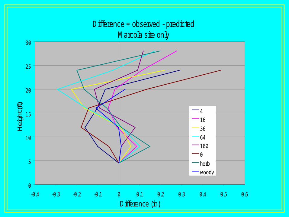
Difference = observed - predictedMarcola site only

0

5

10

15

20

25

30

-0.4 -0.3 -0.2 -0.1 0 0.1 0.2 0.3 0.4 0.5 0.6

Difference (in)

Hei

ght (

ft)

4

16

36

64

100

0

herb

woody

Difference = observed - predictedSummit site only

0

5

10

15

20

25

30

-0.7 -0.6 -0.5 -0.4 -0.3 -0.2 -0.1 0 0.1 0.2

Difference (in)

Hei

ght (

ft)

4

16

36

64

100

0

herb

woody

Potential for systematic bias by treatment

To test for treatment effects on stem profile,

mixed-effects linear and non-linear models

start

finish

Analysis:

Kozak variable exponent model

Dob/DBH = XC

where X = [1-(h/H)0.5] / [1-(4.5/H)0.5]

C = b1(h/H) + b2(h/H)2

Fitted to each individual tree, then SUR for

b1 = f( site, treatment, tree attributes )

b2 = g( site, treatment, tree attributes )

Tentative conclusions:

No treatment effects, but significant site effects.

Relative stem profiles similar even without accounting for differences in height and diameter.