do police reduce crime a reexamination of a natural
TRANSCRIPT
1
Do Police Reduce Crime? A Reexamination of a Natural Experiment*
John J. Donohue† Daniel E. Ho‡ Patrick Leahy§ Stanford Law School Stanford Law School Stanford Law School
Abstract We reexamine a natural experiment first studied by Di Tella and Schargrodsky (2004, “DS”). In response to a 1994 terrorist attack against a Jewish Community Center in Buenos Aires, the government implemented 24-hour police surveillance on city blocks with Jewish institutions. Using a control group of blocks without Jewish institutions, DS applied difference-in-differences, finding that increased policing substantially reduced car theft. We explain how the reallocation of police resources from unprotected to protected blocks, shifts in criminal activity to avoid 24-hour police patrols, and a parking prohibition on protected blocks undermine the original design. The intervention may have displaced, rather than deterred, crime, invalidating the original control group. To investigate this possibility, we reanalyze the data with two modifications. First, we disaggregate the original control group into near and far blocks, with displacement much more likely to affect near blocks. Second, to reduce model sensitivity, we match exactly on all covariates, including neighborhood and the full pretreatment car theft time series. Consistent with displacement, we find that crime increases on near blocks relative to protected blocks, but that crime rates on protected and far blocks are indistinguishable.
I. Introduction Do police reduce crime? Assessing the policing effect has vexed scholars for generations. Governments may deploy police to areas with expected high crime, seriously confounding observational inference. To break the simultaneity of crime and police, one approach has been to * We thank Andrea Chin, Alex Holtzman, Tim Shapiro, and Olga Zverovich for research assistance, Rafael Di Tella and Ernesto Schargrodsky for data, and Jennifer Arlen, Yun-chien Chang, Daniel Chen, Ming-Jen Lin, Dan Rubinfeld, two anonymous referees, and participants at the International Conference on Empirical Studies of Judicial Systems at Academia Sinica for helpful comments. † J.D., Harvard Law School; Ph.D. in Economics, Yale University. C. Wendell and Edith M. Carlsmith Professor of Law; Stanford Law School, Address: 559 Nathan Abbott Way, Stanford, CA 94305; Email: [email protected]. ‡ J.D., Yale Law School; Ph.D. in Government, Harvard University. Professor of Law, Stanford Law School; Address: 559 Nathan Abbott Way, Stanford, CA 94305; Email: [email protected], URL: http://dho.stanford.edu. § M.S. in Statistics, Stanford University. Research Fellow, Stanford Law School; Address: 559 Nathan Abbott Way, Stanford, CA 94305; Email: [email protected].

2
exploit natural experiments that affect police levels in ways unrelated to expected crime. Researchers, for example, have studied electoral cycles,1 tsunamis,2 terror alert levels,3 terrorist attacks,4 and federal grants to police agencies as inducing plausibly exogenous variation in policing to credibly assess its effect.5 We reexamine one such natural experiment first studied by Di Tella and Schargrodsky (“DS”) (2004).6 On July 18, 1994, a Renault van loaded with explosives detonated in front of a major Jewish Community Center in Buenos Aires, Argentina. Eighty-five individuals were killed, hundreds were injured, and the five-story building ultimately collapsed. In the aftermath of the attack, the government began providing 24-hour police protection for 287 Jewish and Muslim institutions in Buenos Aires Province (for fear of reprisals, in the latter case).7 DS used the government’s response to assess the causal effect of police on crime. Since the assignment of police officers was plausibly exogenous to underlying crime levels, this policy provides a potential opportunity to identify the causal effect of a “fixed and observable police presence” on criminal behavior.8 Employing a difference-in-differences (“DID”) approach, DS compared ordinary car theft rates before and after the attack on (1) city blocks with buildings under 24-hour protection (“protected” or “treatment” blocks) and (2) blocks that did not receive special protection (“unprotected” or “control” blocks). They found “a large deterrent effect of observable police on crime” but that “[t]he effect is local, with no appreciable impact outside the narrow area in which the police are deployed.” In this chapter, we revisit this evidence. We argue that there are three mechanisms that may invalidate the experiment. First, the reassignment of police officers to protection details may have reduced police levels in unprotected blocks. Second, the 24-hour police presence on protected blocks may have displaced car thieves from protected to unprotected blocks. Third, a federal order prohibiting parking near potential targets confounds the intervention. Each of these invalidates the assumption that control blocks are independent from the treatment blocks. We
1 See Steven D. Levitt, Using Electoral Cycles in Police Hiring to Estimate the Effects of Police on Crime, 87 AM. ECON. REV. 270 (1997). See also Justin McCrary, Using Electoral Cycles in Police Hiring to Estimate the Effects of Police on Crime: Comment, 92 AM. ECON. REV. 1236 (2002); Steven D. Levitt, Using Electoral Cycles in Police Hiring to Estimate the Effects of Police of Crime: Reply, 92 AM. ECON. REV. 1244 (2002). 2 See Panu Poutvaara & Mikael Priks, The Effect of Police Intelligence on Group Violence: Evidence from Reassignments in Sweden, 93 J. PUB. ECON. 403 (2009). 3 See Jonathan Klick & Alexander Tabarrok, Using Terror Alert Levels to Estimate the Effect of Police on Crime, 48 J.L. & ECON. 267 (2005). 4 See Mirko Draca, Stephen Machin & Robert Witt, Panic on the Streets of London: Police, Crime, and the July 2005 Terror Attacks, 101 AM. ECON. REV. 2157 (2011). 5 See William N. Evans & Emily G. Owens, COPS and Crime, 91 J. PUB. ECON. 181 (2007). 6 See Rafael Di Tella & Ernesto Schargrodsky, Do Police Reduce Crime? Estimates Using the Allocation of Police Forces After a Terrorist Attack, 94 AM. ECON. REV. 115 (2004). 7 Di Tella & Schargrodsky, supra note 6, at 117. 8 Id. at 123.
3
provide evidence consistent with displacement, although ultimately we conclude that the existing data do not lead to firm inferences. The chapter proceeds as follows. Section II provides an overview of the Buenos Aires data and the original DS analysis. Section III discusses threats to validity of the DID design. Section IV describes an alternative DID approach that (a) disaggregates control blocks into “near” blocks that are likely subject to displacement and “far” blocks that are not, and (b) matches treatment, near, and far blocks exactly on all pretreatment covariates, including neighborhood and pretreatment crime trends. Section V presents results consistent with displacement. Crime trends on protected and far blocks are indistinguishable, while crime increases on near blocks. Section VI concludes with a general note of caution about qualitative assumptions underpinning natural experiments. II. Buenos Aires Data and DS Analysis The Buenos Aires data consist of monthly car thefts from April to December 1994 in three neighborhoods with a substantial number of Jewish institutions, out of a total of 48 city neighborhoods.9 The units of analysis are 876 city blocks, 37 of which contained protected buildings. Figure 5.1 shows maps of the three neighborhoods (Belgrano, Villa Crespo, and Oncé), as well as the locations of blocks with protected buildings (solid dots).10 The core of the DS analysis focused on the following model, estimated using ordinary least squares:
where yit is the number of thefts on block i in month t (with fractional thefts when the exact location was unclear); Tit = 1 block i contained a protected building and t > 7 (i.e. after July), and zero otherwise; Mt is a month fixed effect; and Fi is block fixed effect. The coefficient α represents the deterrent effect of police protection on the rate of car thefts. DS found that police protection caused a statistically significant reduction of approximately 0.08 car thefts per month on protected blocks.11 To test whether the protective halo extended to other blocks (but not to test for displacement), DS also tested models with indicators for blocks that were one to two blocks away from protected institutions, but found no evidence for a diffusion of benefits.
9 For many car thefts the reported location is an intersection, rather than a particular block; in these cases DS assigned 0.25 car thefts to each of the adjacent blocks. 10 The original data contain the street name and first address for each block, but no coordinate information. We used the Google Geocoding API to obtain coordinates for the approximate midpoint of each block. 11 DS employed a variety of robustness tests, such as estimating separate treatment effects for each month after the intervention, activating police dummies in earlier months to test whether crime trends in protected blocks were already diverging, and excluding blocks with no thefts in any month under observation. See Di Tella & Schargrodsky, supra note 6, at 124. None of their checks account for displacement, however.
E(yit ) =α Tit +Mt +Fi,

4
Figure 5.1 Neighborhoods Included in Buenos Aires Data
The top right panel shows the location of the three neighborhoods within Buenos Aires. The other three panels zoom in on individual neighborhoods. Gray dots indicate blocks with Jewish institutions, which are disproportionately located in Villa Crespo and Oncé.
Figure 5.2 conveys the intuition of the original findings, plotting average monthly car thefts per block from April to December 1994. The top panel presents theft rates for protected blocks – i.e., blocks that would receive added police protection beginning in August – while the middle panel presents theft rates for unprotected blocks – i.e., blocks serving as the control group. The bottom panel shows monthly averages and 95% pointwise confidence bands for protected blocks (light gray) and unprotected blocks (dark gray). Mean car theft levels on protected and unprotected blocks are somewhat comparable prior the attack. After the attack, the mean rate decreases for protected blocks, but also increases for the large group of unprotected blocks.
Belgrano Block with Jewish institution
Villa Crespo
Site ofattack
Oncé

5
Figure 5.2 Monthly Car Theft Rates
The top panel plots car theft rates for protected blocks (those that received police protection after July) in each month from April to December 2004. The middle panel shows theft rates for unprotected blocks (those that did not receive additional protection after July). Each dot represents one block. Dots are jittered for visibility. The bottom panel plots mean monthly car theft rates for each group of blocks, with pointwise 95% confidence bands. Car thefts occurring between July 18 and July 31 are excluded, as in DS. Theft rates are normalized to 30-day months.
III. Credibility of Identifying Assumptions The central question is whether the decrease in crime on protected blocks can be attributed to deterrence – i.e., whether police protection prevented crimes that otherwise would have occurred. The DID design theoretically allows one to answer this question by using the control group (of
Blocks with Added Police Protection after JulyCa
r The
fts p
er M
onth
0.0
0.5
1.0
1.5
2.0
2.5
Apr May Jun Jul Aug Sep Oct Nov Dec
Added Police Protection
Blocks without Added Police Protection
Car T
hefts
per
Mon
th0.
00.
51.
01.
52.
02.
5
Apr May Jun Jul Aug Sep Oct Nov Dec
Average Car Theft Rates
Mea
n Ca
r The
fts p
er M
onth
Unprotected Blocks
Protected Blocks
0.00
0.05
0.10
0.15
Apr May Jun Jul Aug Sep Oct Nov Dec

6
unprotected blocks) to estimate counterfactual potential outcomes for protected blocks (absent the protection policy). Unprotected blocks must still satisfy two conditions, however, in order to serve as a valid control group: (a) they must be independent of the treatment received by the protected blocks, and (b) exhibit homogeneity in time trends with protected blocks. We argue that both of these assumptions are likely not met. A. Independence One general difficulty in attributing changes to the protection policy is that it did not occur in isolation: the city had just weathered the deadliest terrorist attack in Argentina’s history,12 which could have affected crime in many other ways. Terrorist attacks have been noted to have a wide and unpredictable impact on economic activity and human behavior.13 Ignoring broader social effects, we identify three ways in which the government’s response might have impacted crime on unprotected blocks, violating the assumption of independence. First, the attack almost certainly affected police levels on unprotected blocks. Officers cannot be drawn from thin air. The provision of 24-hour police protection on certain blocks likely decreased the police resources available to others. According to DS “the police forces made a serious effort to maintain previous levels of police presence in the rest of the neighborhoods,” but “more than one-third of approximately 200 police officers stationed in Once [sic]… had to be reassigned to protection duties.”14 Other security measures may have absorbed additional police resources in these neighborhoods,15 and there may also have been a large-scale shift in police priorities from combatting street crime to preventing terrorism.16 Independent of any shift in criminal activity, a reduction in police levels – or a decreased emphasis on apprehending ordinary criminals – would theoretically lower the risks associated with crime and thereby incite car thieves to act with greater frequency.17 Alternatively, of course, it is possible that police levels increased throughout these neighborhoods as the government tightened security and shifted police resources toward neighborhoods with a large Jewish population. Either scenario, 12 See Michael Warren, Israel Concerned over Argentina-Iran Meetings, SEATTLE TIMES, Sept. 28, 2012, http://seattletimes.com/html/nationworld/2019291408_apltargentinairanisrael.html. 13 See, e.g., Seymour Spilerman & Guy Stecklov, Societal Responses to Terrorist Attacks, 35 ANN. REV. SOC. 167 (2009); Zvi Eckstein & Daniel Tsiddon, Macroeconomic Consequences of Terror: Theory and the Case of Israel, 51 J. MONETARY ECON. 971 (2004); Gary S. Becker & Yona Rubinstein, Fear and the Response to Terrorism: An Economic Analysis (Feb. 2011) (unpublished manuscript) (on file with authors). 14 Di Tella & Schargrodsky, supra note 6, at 117. 15 The government also instituted air patrols and heightened security at media buildings and airports, for instance. See British Broad. Corp., Government Adopts Security Measures in View of Possible Terrorist Attack, BBC SUMMARY OF WORLD BROADCASTS, Aug. 15, 1994. 16 Soon after the attack, for instance, Argentina’s president created a new security agency “to oversee police and quasi-military institutions.” Martin Andersen, A New Security Force Rises from the Ashes in Argentina, WASH. TIMES, Aug. 22, 1994. See also Calvin Sims, Argentina’s New Secret Security Agency Raises Fear of Repression, HOUSTON CHRON., Sept. 11, 1994. 17 A redistribution of police has been noted in a few cases to at least be correlated with an increase in crime: rates of street crime in London, for example, peaked in the month after the September 11 attacks, when police were redeployed to secure potential terrorist targets. Reportedly, robberies also increased in London when police were redeployed during a visit by President Bush in 2003. KATHRYN CURRAN ET AL., CRIME AND DRUGS DIVISION, GOVERNMENT OFFICE FOR LONDON, STREET CRIME IN LONDON: DETERRENCE, DISRUPTION, AND DISPLACEMENT (2005).

7
however, would result in biased estimates of the deterrent effect. Without data on police levels, it is impossible to know what effects we are actually measuring when comparing protected and unprotected blocks. Second, criminals may have responded to the police presence on protected blocks by refocusing their activities on unprotected blocks. Spatial displacement is a common concern with crime prevention measures that focus on particular locations: increasing enforcement efforts in one area may displace criminals to others (or to other types of crime, a possibility that we have no way of examining).18 Empirical findings about the prevalence of displacement have been mixed,19 but in the current case, it is doubtful that thieves would be limited by a lack of opportunity on other blocks, given the ubiquity of vehicles. In the four months prior to the attack, a car theft was reported on or at the intersection of 51% of the blocks under observation, suggesting that opportunities for theft are not geographically restricted to a few hot spots. This possibility is especially likely if police levels decreased—or even were perceived to decrease—on blocks without Jewish institutions. It is thus conceivable that crime would, as the authors of one study on displacement put it, literally “move around the corner.”20 Last, the intervention may have altered the distribution of vehicles themselves, leading to changes in car theft patterns. In the wake of the attack, the government imposed parking restrictions on the streets of protected institutions, potentially dislocating cars and traffic and reducing the number of available targets on protected blocks.21 The 24-hour police protection is fundamentally confounded with the parking prohibition. While DS estimate that a small fraction of parking space on protected blocks was affected by the prohibition,22 little evidence exists to corroborate its scope. In any case, the number of vehicles on blocks with Jewish institutions may also have decreased if they were perceived as potential terrorist targets.23 And there would have been an acute parking disruption in the area around the site of the bombing itself, which is included in the DS analysis. B. Homogeneity
18 See, e.g., Thomas A. Reppetto, Crime Prevention and the Displacement Phenomenon, 22 CRIME & DELINQUENCY 166 (1976). 19 See Rob T. Guerette & Kate J. Bowers, Assessing the Extent of Crime Displacement and Diffusion of Benefits: A Review of Situational Crime Prevention Evaluations, 47 CRIMINOLOGY 1331 (2009). 20 David Weisburd et al., Does Crime Just Move Around the Corner? A Controlled Study of Spatial Displacement and Diffusion of Crime Control Benefits, 44 CRIMINOLOGY 549 (2006). 21 According to one press report, “the Federal Police has been ordered not to allow the parking of vehicles outside any objective on any account.” British Broad. Corp., supra note 15. 22 See Di Tella & Schargrodsky, supra note 6, at 124. 23 This was a reasonable fear given that the 1994 attack was not an isolated incident: a similar bombing had occurred at the Israeli Embassy in Buenos Aires two years earlier. and in August 1994 the government received warnings that yet another attack was imminent, leading to heightened security – bomb-sniffing dogs and armored vehicles – at some Jewish institutions. Menem Warns Argentinians Against Bomb Panic, JERUSALEM POST, Aug. 14, 1994.

8
Random assignment of protection would guarantee that protected and control blocks follow (in expectation) comparable underlying time trends. The assignment of police protection, however, was determined by the location of Jewish (and Muslim) institutions. As a result, there may be systematic differences between the control and treatment groups. One obvious difference, as Figure 5.1 shows, is that protected blocks are disproportionately located in Oncé and Villa Crespo (and are often clustered together within neighborhoods as well), while Belgrano contains the majority (55%) of unprotected blocks under observation. Crime varies considerably across neighborhoods, however: in the pretreatment period, Oncé, Villa Crespo and Belgrano had 0.04, 0.08, and 0.11 thefts per block (F-test p-value < 0.0001). The imbalance means that crime trends -- estimated largely from Belgrano -- may not be homogeneous across treatment and control groups, potentially biasing results.24 Indeed, the pretreatment time series itself suggests a lack of homogeneity, as protected and unprotected blocks appear to diverge even in the pretreatment period.25
* * *
Natural experiments require assumptions that must be defended. In the Buenos Aires case, there are strong substantive reasons to think that the independence assumption is violated. Displacement, rather than deterrence, may drive the decrease in crime that DS observe. While the available data may not allow us to learn much more, we demonstrate one possible research design that attempts to account for displacement effects, weaken model sensitivity, and establish more homogeneous treatment and control groups. We emphasize, however, that the primary purpose of this chapter is to raise questions about the deterrence effect in the Buenos Aires data. IV. An Alternative Approach A. Constructing a Plausible Control Group We modify DS’s approach in two ways to address the implausibility of the independence and homogeneity assumptions. First, we disaggregate unprotected blocks into two groups: “near” blocks, which are within one to three blocks of a protected institution, and “far” blocks, which are located four or more blocks away. Near blocks are presumably more likely to be affected by at least two of the three mechanisms discussed above: crime-shifting in response to the police presence and the parking 24 Consider the following simplified scenario: neighborhood A has 100 control blocks and 5 treated blocks, while neighborhood B has 20 control and 20 treated. If crime increases by 1 unit on every block in neighborhood A, and does not change at all in neighborhood B, the average increase across all control blocks is 100/120 = 0.83 units, while across all treated blocks it is 20/40 = 0.5 units. Even though there is no deterrent effect in either neighborhood, we observe an apparent one when outcomes are averaged across neighborhoods. 25 For instance, with a conventional DID approach for just the June and July data, we would reject the null hypothesis of no deterrence effect at a 10% level, despite the fact that the test is conducted on data exclusively prior to the police intervention.

9
prohibition. There is of course no obvious threshold between near and far blocks, but it seems plausible that drivers unable to park on protected blocks and thieves displaced by 24-hour patrols would be displaced in only a localized way. Our cutoff classifies 557 blocks as near and 279 as far.26 (We exclude the block where the attack occurred and all adjacent blocks, which were impacted in a more drastic way by cleanup and building reconstruction.27) Second, to make the homogeneity assumption more credible (and to reduce model dependence), we preprocess the data by matching protected, near, and far blocks that are identical in all pretreatment covariates. 28 In essence, we construct strata with identical values on eight covariates: the neighborhood; thefts rates in each of the pretreatment months (March to the beginning of July); and the presence of a bank, gas station, or public institution.29 The latter three, as DS note, may have an independent deterrent effect on car thefts. 30 Matching on the neighborhood ensures that groups are physically proximate, and avoids using the large number of high-crime, control blocks in Belgrano to estimate counterfactual outcomes for protected blocks disproportionately in the other neighborhoods. Matching units with identical pretreatment car theft time series means that any posttreatment deviation between groups can be more plausibly attributed to the intervention. Matching produces nine strata (listed in Appendix A) with common support, containing 307 blocks (21 protected, 218 near, and 68 far). To estimate the (in-sample) treatment effect on the protected blocks, we construct matching weights proportional to the number of protected blocks in each stratum (e.g., a stratum with i protected, j near, and k far blocks results in weights of 1, i/j, and i/k, respectively). Table 1 summarizes covariate balance for the raw and matched samples. Protected, near, and far blocks have different neighborhood distributions in the raw sample. Moreover, the average June theft rate is substantially higher for protected blocks than near or far blocks. By construction, exact matching results in perfect covariate balance in these dimensions.
26 Since DS include controls for observations at a distance of one or two blocks, our threshold only extends the radius of possible influence by a block. Roughly 20% of the sample is three blocks away from a protected institution, however, so this expansion removes a large number of blocks from the control group. 27 The block where the attack occurred is also an invalid treatment unit because the Jewish Community Center was under police protection prior to the terrorist attack, due to a similar bombing at the Israeli embassy in 1992. According to a news report, “a police car was permanently stationed in front of the building.” The car was destroyed in the explosion and two police officers were killed. Federico Ferber, Argentina: Bombed Jewish Building Had Poor Security, INTER PRESS SERV. (July 19, 1994). 28 See Daniel E. Ho et al., Matching as Nonparametric Preprocessing for Reducing Model Dependence in Parametric Causal Inference, 15 POL. ANALYSIS 199 (2007); Stefano M. Iacus, Gary King & Giuseppe Porro, Causal Inference with Balance Checking: Coarsened Exact Matching, 20 POL. ANAL. 1 (2012). 29 This procedure is a form of coarsened exact matching, where we “coarsen” the time series for each block to the month level to facilitate matches. See Iacus, King & Porro, supra note 28. 30 See Di Tella & Schargrodsky, supra note 6, at 128.

10
Table 5.1 Covariate Balance in the Raw and Matched Samples Raw Sample Matched Sample Protected Near Far Protected Near Far Neighborhood Belgrano 0.20 0.41 0.82 0.19 0.19 0.19 Villa Crespo 0.37 0.36 0.16 0.33 0.33 0.33 Oncé 0.43 0.23 0.03 0.48 0.48 0.48 Crime Rates April 0.13 0.13 0.08 0.00 0.00 0.00 May 0.09 0.10 0.10 0.03 0.03 0.03 June 0.14 0.07 0.08 0.08 0.08 0.08 July 0.04 0.07 0.07 0.02 0.02 0.02 Buildings Bank 0.06 0.08 0.08 0.10 0.10 0.10 Gas Station 0.03 0.02 0.03 0.00 0.00 0.00 Public Inst. 0.06 0.04 0.02 0.00 0.00 0.00 Blocks 35 557 279 21 218 68
Columns summarize the covariates used for matching in each group of blocks – protected, near, and far – within the full sample and matched sample. The rows under “Neighborhood” contain the average value of dummy variables indicating whether each block is in a particular neighborhood. (Due to rounding, the three values may not sum to 1.00.) The rows under “Crime Rates” contain the average monthly theft rate in each month prior to the attack. The rows under “Buildings” contain the average value of dummy variables indicating the presence of each building type. For the matched sample, all figures are weighted averages. By construction, covariates have the same mean value across all groups in the matched sample.
Removing observations for unmatched blocks (i.e., observations with no common support), we estimate the effects of the intervention via weighted least squares, minimizing:
where is the weight assigned to block i; is an indicator variable for protected blocks in
months after the intervention, is an indicator for near blocks in months after the intervention; and fixed effects are as before. The coefficient α represents the effect of the intervention on protected blocks and β its effect on unprotected nearby areas, relative to the control group of far blocks. We might interpret negative and positive values of these coefficients as deterrent and displacement effects, respectively. (In the discussion that follows, we use the term “displacement” somewhat loosely to refer to an increase in crime driven by proximity to protected blocks, regardless of the precise mechanism responsible.) B. Results
€
wi yit − αTitprot + βTit
near + Mt + Fi( )[ ]i,t∑ ,
€
wi Titprot
€
Titnear

11
Table 2 reports estimates of these effects, with robust standard errors in parentheses. The first column presents results for the full matched sample, with treatment effects pooled across neighborhoods. The deterrent effect (for protected blocks) is statistically indistinguishable from zero. The displacement effect (for near blocks) is positive and statistically significant. We estimate that the added police patrols caused an increase in 0.06 car thefts per block per month, plus or minus 0.04, at the 95% confidence level. This amounts to roughly 13 thefts per month across all near blocks in the matched sample. The next three columns of Table 2 present results for matched blocks within a single neighborhood. Displacement effects appear in Villa Crespo and Oncé, but not in Belgrano. Deterrence effects are never statistically significant.
Table 5.2 Effects of the Protection Policy Pooled Belgrano Villa Crespo Oncé Protected x Post -0.014
(0.017) -0.087
(0.076) 0.008
(0.016) 0.000
(0.010) Near x Post 0.061
(0.019)** 0.033
(0.089) 0.072
(0.013)*** 0.065
(0.013)*** N 2763 450 1296 1017 Adjusted R2 0.10 0.10 0.08 0.10
The first column presents weighted least squares regression results for the full matched sample. The remaining columns present results for the model when fitted using only matched observations in a single neighborhood. “Protected x Post” is the effect of the intervention on treated blocks; “Protected x Near” is the effect on near blocks. The dependent variable is the number of car thefts per month per block. All regressions include block and month fixed effects. Robust standard errors are given in parentheses. ** = significant at the 0.01 level. *** = significant at the 0.001 level.
Figure 5.3 illustrates these findings, plotting months on the x-axis against car theft rates on the y-axis, separately for protected, near, and far blocks in the matched sample. The three lines represent monthly weighted averages of the theft rate in each group, with 95% pointwise confidence intervals.31 By construction, the three groups have identical trends before the attack. In the aftermath of the terrorist attack, the theft rate rises in near blocks, diverging sharply from the other two groups, while protected and far blocks remain indistinguishable in the months immediately after the attack.
31 As in DS, the averages for July include only the first 17 days of the month.

12
Figure 5.3 Monthly Car Theft Rates in the Matched Sample
The three lines show weighted averages of the monthly car theft rate in each group of blocks in the matched sample (using the weights described in Section IV). Thefts from July 18 to July 31 are excluded from the July averages. Theft rates are normalized to a 30-day month. By construction, the three trend lines are identical in months before the attack. After the attack, the theft rate rises among near unprotected blocks.
What explains the discrepancy between these results and the deterrence effect that DS found? The DS model restricts the coefficient on nearby blocks by pooling near and far blocks32 and assigns a weight of 1 to each observation. This has two effects. First, pooling nearby blocks (where crime rises) and far blocks (where crime stays the same as in protected blocks) in the control group inflates the estimated deterrent effect, since the difference is just as plausibly due to displacement effects. Second, equal weighting means that Belgrano, which has a higher baseline rate of car thefts, has a disproportionate influence on the results, despite the fact it has the smallest number of protected blocks. Villa Crespo and Oncé, on the other hand, have relatively low theft rates, such that there is not much crime to deter. Indeed, Belgrano drives DS’s original findings: if Belgrano is omitted from their models, the estimated deterrent effect is statistically insignificant decrease of roughly 0.05 car thefts per month (compared to a 0.18 decrease in Belgrano33).
32 To be precise, DS in some specifications test for a protective halo by including controls for units one to two blocks away, but find these to be statistically insignificant. The key pooling assumption is for blocks that are three blocks away and more than three blocks away. 33 The Belgrano effect is statistically significantly different from 0 and the effect outside of Belgrano.
0.00
0.05
0.10
0.15
Mea
n Ca
r The
fts
Apr May Jun Jul Aug Sep Oct Nov Dec
ProtectedNear, UnprotectedFar, Unprotected

13
Figure 5.4 Car Theft Rates on Matched Blocks Before and After the Attack
Each vertical panel shows outcomes for one of the groups in the matched sample. Within each panel, the two columns show average monthly crime rates for individual blocks in that group before and after the attack. Black dots indicate the location of matched blocks. The gray circles are sized in proportion to the overall theft rate for that period.
To visualize these neighborhood differences, Figure 5.4 plots outcomes in the matched sample before and after the intervention for each neighborhood. Black dots indicate the location of matched blocks while the gray circles are proportional to the car theft rate for the pre and post-period. In Belgrano, matched blocks each experience thefts pre-attack; afterward, thefts decline somewhat in protected blocks but remain roughly constant in the two unprotected groups. In the other two neighborhoods, by contrast, we see a sharp increase in near blocks and virtually no change in far blocks. Because matched blocks in these neighborhoods mostly had no car thefts prior to the attack, we might expect thefts to increase by regression to the mean. But the increase is concentrated almost entirely in areas closer to protected blocks, suggesting that displacement may be driving these car thefts. Lastly, we offer some evidence of displacement in the raw sample. Figure 5.5 presents 30-day moving averages of the crime rate across all near and far unprotected blocks. The theft rates are remarkably consistent, crisscrossing frequently, for most of the observation period, but diverge in the two months after the attack. This divergence appears consistent, at least, with the displacement of car theft to near blocks.
Protected Near, Unprotected Far, UnprotectedBefore After Before After Before After
Belg
rano
Villa
Cre
spo
Onc
é
●
●
●
●
●
●
●
●
●
●
●
●
●
●
●
●
●
●
●
●●
●
●
●
●
●
●
●
●
●
●
●
●
●
●
●
●
●
●
●
●●
●
●
●
●
●
●
●
●
●
●
●
●
●
●
●
●●
●
●
●
●
●
●
●
●
●
●
●
●
●
●
●
●●
●
●
●
●
●
●
●
●
●●●
●
●
●
●
●
●
●
●●
●●
●
●
● ●●
●
●
●
●
●
●●
●●
●
●
●●
●●
●●
●
●
●
●
●
●
●
●●
●●
●
●
●
●
●
●●
●
●●
●
●●
●●
●●
●●
●
●
●●
●●
●
●●
●●
●
●
●
●●
●●
●
●●
●
●
●
●
●
●
●
●
●
●
●
●
●
●●
●
●
●
●
●
●●
●
●
●●
●
●
●
●
●
●
●
●
●
●
●
●
●
●
●
●●
●●
●
●
●
●
●
●
●
●
●
●
●
●
●
●
●
●
●
●
●
●
●
●
●
●
●
●
●
●
●
●
●
●
●
●
●
●
●
●
●
●
●
●
●
●
●
●
●
●
●●
●●●●●●●
●●●●●
●●●●●
●●●●●●●●●
●●●●
●●●●●● ●●●●●
●●●● ●●
●
●●
●
●
● ●●
●
●
●
●
●
●●
●●
●
●
●●
●●
●●
●
●
●
●
●
●
●
●●
●●
●
●
●
●
●
●●
●
●●
●
●●
●●
●●
●●
●
●
●●
●●
●
●●
●●
●
●
●
●●
●●
●
●●
●
●
●
●
●
●
●
●
●
●
●
●
●
●●
●
●
●
●
●
●●
●
●
●●
●
●
●
●
●
●
●
●
●
●
●
●
●
●
●
●●
●●
●
●
●
●
●
●
●
●
●
●
●
●
●
●
●
●
●
●
●
●
●
●
●
●
●
●
●
●
●
●
●
●
●
●
●
●
●
●
●
●
●
●
●
●
●
●
●
●
●●
●●●●●●●
●●●●●
●●●●●
●●●●●●●●●
●●●●
●●●●●● ●●●●●
●●●● ●●
●
●
●
●
●
●
●
●
●
●●
●
●
●
●
●
●
●
●
●
●
●
●
●
●
●
●
●
●
●
●
●
●
●●
●
●
●
●
●
●
●
●
●
●
●
●
●
●
●
●●
●
●
●
●
●
●
●
●
●
●
●
●
●
●
●
●
●
●
●
●
●
●
●
●
●
●
●
●
●
●
●●
●
●
●
●
●
●
●
●
●
●
●
●
●
●
●
●
●
●
●
●●
●●
●
●
●
●
●
●
●
●
●
●
●
●
●
●
●
●
●
●
●
●
●
●
●
●
●
●
●
●
●
●
●
●
●
●
●
●
●
●
●
●
●
●
●
●
●
●
●
●
●●
●●●●●●●
●●●●●
●●●●●
●●●●
●●●●●
●●●●
●●●●●●
●●●●●
●●●● ●●
●
●
●
●
●
●
●
●●
●
●
●
●
●
●
●
●
●
●
●
●
●
●
●
●
●
●
●
●
●
●
●
●
●
●
●
●
●
●
●
●
●
●
●
●
●
●
●
●
●
●
●
●
●
●
●
●
●
●
●
●
●
●
●
●
●
●
●
●
●
●
●
●
●
●
●●
●●●●●●●
●●●●●
●●●●●
●●●●
●●●●●
●●●●
●●●●●●
●●●●●
●●●●
●●
●
●
●
●
●
●
●
●
●●
●
●
●
●
●
●
●
●
●
●
●
●
●
●
●
●
●
●
●
●
●
●
●●
●
●
●
●
●
●
●
●
●
●
●
●
●
●
●
●
●
●
●
●
●
●
●
●
●
●
●
●
●
●
●
●
●
●
●
●
●
●
●
●
●
●
●
●
●
●
●
●
●
●
●
●
●
●
●
●
●
●
●
●
●
●
●
●
●
●
●
●
●●
●
●●
●
●
●
●
●
●
●
●
●
●
●
●
●
●
●
●
●
●
●
●
●
●
●
●
●
●
●
●
●
●
●
●
●
●
●
●
●
●
●
●
●
●
●
●
●
●
●
●●
●●●●●●●
●●●●●
●●●●●
●●●●
●●●●●
●●●●
●●●●●●
●●●●●
●●●●
●●
●
●●
●●
●●
●●
●
●
●
●●
●
●●
●
●●
●
●
●
●●
●
●
●
●
●
●
●●
●
●
●
●
●●
●●
●
●●
●
●
●●
●
●
●●
●
●
●
●
●
●
●
●
●
●
●
●●●
●●
●●
●●
●●
●
●
●
●●
●
●●
●
●●
●
●
●
●●
●
●
●
●
●
●
●●
●
●
●
●●
●●
●
●●
●
●
●●
●
●
●●
●
●
●
●
●
●
● ●
●
●
●
●
●
●
●
●
●
●
●
●
●
●
●
●
●
●
●
●
●
●
●
●
●
●
●
●
●
●
● ●
●
●
●
●
●
●
●
●
●
●
●
●
●
●
●
●
●
●
●
●
●
●
●
●
●
●
●
●
●
●
●
●
●
●
●
●
●
●
●
●
●
●
●
●
●
●
●
●
●
●
●
●
●
●
●
●
●
●
●
●
●
●
●
●
●
●
●
●
●
●
●
●
●
●
●
●●
●●●●
●
●
●
●
●
●
●
●
●
●
●
●
●
●
●
●
●
●
●
●
●
●
●
●
●
●
●
●
●
●
●
●
●
●
●
●
●
●
●
●
●
●
●
●
●
●●
●●●●
● ●0 car thefts per month 0.25 car thefts per month

14
Figure 5.5 30-Day Moving Averages of Theft Rate in Near and Far Blocks
The two lines represent daily time series for near and far blocks. For a given day the height of each line corresponds to the average number of thefts on near or far blocks within a 30-day window centered on that day.
* * *
With a few seemingly innocuous modifications to the original approach -- aimed to make more credible the independence and homogeneity assumptions -- we find evidence inconsistent with pure deterrence. Of course, the affirmative evidence of displacement is also limited: there are fewer units with common support; the time series is very short, making it difficult to establish homogeneity in the pretreatment period; and without further knowledge about the precise mechanisms at work, far blocks, as we have defined them, may not be a persuasive control group. At minimum, however, this reanalysis establishes that the conclusions one draws from the data depend considerably on the qualitative assumptions one is willing to make. V. Conclusion Our reexamination of the Buenos Aires experiment questions DS’s finding of a deterrent effect. There are strong reasons to suspect that the 24-hour police protection policy displaced crime to other blocks. The Argentinian natural experiment may be less a story of the deterrent effect of police than of the complex and inadvertent impact of anti-terrorism measures on street crime. Firmer conclusions would require both (a) more precise data and (b) deeper institutional and historical knowledge. Better Data. First, we would ideally have block-level data on police activity. The analyses above use the presence of a protected institution as a proxy for police presence, but “protected” and “unprotected” blocks are better characterized as blocks on which at least one officer was stationed and blocks about which we have no information on police levels. Police levels may have decreased on unprotected blocks, but the devastation caused by this terrorist attack may
0.00
0.05
0.10
0.15
0.20
Crim
es P
er 3
0 Da
ys P
er B
lock
May Jun Jul Aug Sep Oct Nov Dec
Near
Far

15
also have heightened police vigilance throughout the city. Second, data on parking availability and traffic flows would potentially enable one to separate the effects of police protection from those of the parking prohibition. Third, to establish DID as a credible identification strategy, crime data from a longer observation period would be invaluable, allowing the researcher to examine (and better adjust for) seasonal trends in car thefts. As Appendix B documents, however, obtaining such historical data from Buenos Aires is challenging. Finally, for the research design we propose, additional block-level information on factors that may influence thefts -- such as street size, lighting, foliage, and activity levels -- would help in establishing more credible matches. Institutional Knowledge. Qualitative institutional knowledge is invaluable in assessing the credibility of assumptions and specific causal mechanisms. What was the nature of the added police protection? What precisely were the officers’ duties? How visible were they to would-be thieves? Did protection vary by institution or over time? How widely publicized was the protection policy? What types of car thieves operate in these neighborhoods, and how far might they reasonably travel in search of targets? Obviously, it is not always feasible to acquire all the data and qualitative information that a researcher desires. DS deserve much credit for identifying a case where police assignment was plausibly exogenous to crime, obtaining these data, and conducting interviews with high-level officials. But the DID research design requires the assessment of the credibility of key assumptions that may not be justified in this case.. While DS’s evidence may not be persuasive, we see promise in the use of natural experiments and granular crime data to evaluate police effects. Conventional observational studies in this area often rely on geographically aggregated data, such as police size and budgets and city- or county-level crime rates. 34 While such studies encompass many jurisdictions, causal inference is difficult in such observational settings.35 Moreover, aggregated data may provide less insight into how police reduce crime, given the myriad ways in which police resources can be deployed. The Buenos Aires natural experiment, by contrast, in principle permits researchers to assess the impact of a specific mechanism, namely the observable presence of stationary police officers. As local law enforcement agencies increase the scope, quality, and accessibility of the data they collect, research in this vein will undoubtedly reveal greater nuances in the relationship between police and crime.
34 See Hyeyoung Lim, Hoon Lee & Steven J. Cuvelier, The Impact of Police Levels on Crime Rates: A Systematic Analysis of Methods and Statistics in Existing Studies, 8 ASIA PAC. J. POLICE & CRIM. JUST. 49 (2010). 35 But see Aaron Chalfin & Justin McCrary, The Effect of Police on Crime: New Evidence from U.S. Cities, 1960-2010 (Oct. 1, 2012) (unpublished manuscript) (on file with author).
16
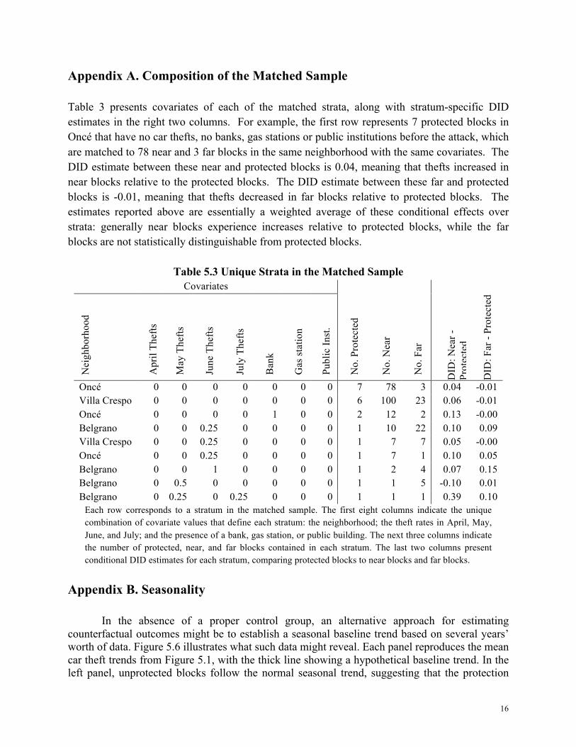
Appendix A. Composition of the Matched Sample Table 3 presents covariates of each of the matched strata, along with stratum-specific DID estimates in the right two columns. For example, the first row represents 7 protected blocks in Oncé that have no car thefts, no banks, gas stations or public institutions before the attack, which are matched to 78 near and 3 far blocks in the same neighborhood with the same covariates. The DID estimate between these near and protected blocks is 0.04, meaning that thefts increased in near blocks relative to the protected blocks. The DID estimate between these far and protected blocks is -0.01, meaning that thefts decreased in far blocks relative to protected blocks. The estimates reported above are essentially a weighted average of these conditional effects over strata: generally near blocks experience increases relative to protected blocks, while the far blocks are not statistically distinguishable from protected blocks.
Table 5.3 Unique Strata in the Matched Sample Covariates
No.
Pro
tect
ed
No.
Nea
r
No.
Far
Nei
ghbo
rhoo
d
Apr
il Th
efts
May
The
fts
June
The
fts
July
The
fts
Ban
k
Gas
stat
ion
Publ
ic In
st.
DID
: Nea
r -
Prot
ecte
d
DID
: Far
- Pr
otec
ted
Oncé 0 0 0 0 0 0 0 7 78 3 0.04 -0.01 Villa Crespo 0 0 0 0 0 0 0 6 100 23 0.06 -0.01 Oncé 0 0 0 0 1 0 0 2 12 2 0.13 -0.00 Belgrano 0 0 0.25 0 0 0 0 1 10 22 0.10 0.09 Villa Crespo 0 0 0.25 0 0 0 0 1 7 7 0.05 -0.00 Oncé 0 0 0.25 0 0 0 0 1 7 1 0.10 0.05 Belgrano 0 0 1 0 0 0 0 1 2 4 0.07 0.15 Belgrano 0 0.5 0 0 0 0 0 1 1 5 -0.10 0.01 Belgrano 0 0.25 0 0.25 0 0 0 1 1 1 0.39 0.10
Each row corresponds to a stratum in the matched sample. The first eight columns indicate the unique combination of covariate values that define each stratum: the neighborhood; the theft rates in April, May, June, and July; and the presence of a bank, gas station, or public building. The next three columns indicate the number of protected, near, and far blocks contained in each stratum. The last two columns present conditional DID estimates for each stratum, comparing protected blocks to near blocks and far blocks.
Appendix B. Seasonality
In the absence of a proper control group, an alternative approach for estimating counterfactual outcomes might be to establish a seasonal baseline trend based on several years’ worth of data. Figure 5.6 illustrates what such data might reveal. Each panel reproduces the mean car theft trends from Figure 5.1, with the thick line showing a hypothetical baseline trend. In the left panel, unprotected blocks follow the normal seasonal trend, suggesting that the protection

17
policy has a purely deterrent effect. In the middle panel, however, it is protected blocks that follow the baseline trend, which suggests the increase in crime among unprotected blocks is due to displacement. In the right panel there is minimal seasonality, implying a mixture of deterrence and displacement.
Figure 5.6 Hypothetical Baseline Trends
Each panel plots actual mean car theft rates for protected (lighter grey) and unprotected (darker grey) blocks, as shown in the bottom panel of Figure 5.1. The thick black lines indicate hypothetical baseline trends. In the left panel, the observed data is most consistent with pure deterrence; in the middle panel with pure displacement; and in the right panel, with both deterrence and displacement. To assess seasonality in Buenos Aires car thefts, we attempted to collect data for a longer
period of time. Using insurance reports from the Superintendencia de Seguros de Nación, we were able to obtain monthly province-level data only from 2008 to mid-2010. Figure 5.7 presents the car theft time series for each province, with the city and province of Buenos Aires. The vertical black line indicates a new calendar year and the grey bands indicate the August-December period, the months corresponding to the treatment period in the DS data. The individual times series exhibit considerable noise: comparing trends in the city of Buenos Aires before and after July would indicate an increase in 2008 but a decrease in 2009. To leverage information from the other provinces, we fit a generalized additive model with year and province fixed effects, allowing for a smooth time trend over the calendar year. The dark gray line in the left panel of Figure 5.7 represents the seasonal trend for Buenos Aires. While the months of January and February generally exhibit decreased car theft (see the top right panel), such systematic seasonality is small compared to the month-to-month noise in car theft: the line is effectively flat. This would seem to point toward the possible presence of both displacement and deterrence in the DS data, but given the large gap in time between the two datasets, it is probably unreasonable to extrapolate time trends from one to the other.
While there is no evidence of strong seasonality, the additional car theft data does point to one danger in the use of DID estimators. When serial correlation is present, estimated standard errors will be smaller than their true values, which may result in the detection of significant effects where none exist. 36 Here, for example, a placebo DID test where we activate the treatment in each possible province at each possible month yields a 13% false positive rate (at a 0.05 significance level), as shown in the bottom right panel of Figure 5.7.
36 See Marianne Bertrand et al., How Much Should We Trust Differences-in-Differences Estimates?, 119 Q. J. ECON. 249 (2004).
Pure Deterrence
Month
Car
The
ft
Pure Displacement
MonthC
ar T
heft
Mixed
Month
Car
The
ft

18
Figure 5.7 Car Theft Trends in Argentina, 2008-2010
The left panel shows monthly car theft rates in Argentinian provinces. The thick black line indicates the estimated seasonal trend (using a generalized additive model smoothing over months). The top right panel zooms in on the seasonal trend. The bottom right panel plots p-values from placebo DID estimates, showing a 13% Type I error rate at the 0.05 significance level.
Regional Time Series
Month
Car t
heft
rate
Seasonal trend
2008 2009 2010
Buenos AiresCity
Buenos AiresProvince
Other provinces
January July January July January
010
2030
40
Seasonal Trend (zoomed)
Month
Car T
heft
Placebo Test Results
p−value
Freq
uenc
y
0.0 0.2 0.4 0.6 0.8 1.0
040
Type Ierror = 0.13