do-it-yourself partial equilibrium modelling david vanzetti division on international trade in goods...
TRANSCRIPT

Do-it-yourself partial equilibrium modelling
David Vanzetti
Division on International Trade in Goods and Services, and Commodities
UNCTAD, Geneva
United Nations Conference on Trade and DevelopmentUnited Nations Conference on Trade and Development
Much of the material for this presentation was compiled by Joseph Francois of the Tinbergen Institute. Several of the models can be downloaded from his website, www.interceonomics.com.

Typical questions
• Who gains from removing export subsidies?
• Is domestic support important?
• Do special/sensitive product exemptions weaken the outcome?

Country-specific questions
• Will we gain or lose from further liberalisation?
• Export enhancement?
• Or flooded with imports?
• Tax revenues?

The need for quantitative analysis
• Policy changes have negative and positive effects.
• Price changes generate winners and losers.
• Quantitative analysis needed to aggregate effects.
• Numbers are needed to support arguments.

Overview
• The policy issue
• Model choices
• Some simple spreadsheet models
• Use and abuse of model results

Incidence of a tax
D
P
Q
S
S’
1
32
7
4
5
6
Domestic production tax.Taxes collected are area 1567.The welfare cost is area 546.This is the sum of the producer loss 2467 andconsumer loss 1542, lesstaxes collected.
© Joe Francois

Large country import tariff
D
P
M
S
Import taxes collected are area 1256. Consumer cost is area 12347. Taxes collected amount to area 1256. The welfare gain equals the difference between consumer losses and taxes. As some taxes (area 7456) come from terms of trade gains, the welfare effects depends on the relative size of 243 and 7456.
12
3
4
567
© Joe Francois

Welfare effects of tariff change
D
P
Q
S
When import tax t is removed, domestic price fall to P. Taxes formerly collected, area 2356, are lost. Consumers gain area 1348. Producers lose area 1278. The welfare gain equals the dead weight losses (DWL), 267 plus 345. These may be offset by a terms of trade effect, a rise in P, not shown hear.
P+t
TR
3
DWL1
P 4
2
6 58 7

Terms of trade effect
Dm
P
Q
Sm
With removal of import tax, Pw must rise to equate imports and exports. Some of te gains of liberalisation are captured by the exporter.
Pw+t
Pw
m0
Sx
Dxx0

Choices
• Homogeneous or heterogeneous product (imperfect substitutes)
• Preferential or multilateral tariff changes• Spatial (bilateral) or non-spatial• Net trade or two way trade• Linear or non-linear• Static or dynamic • Deterministic or stochastic

Spreadsheet models
• Simple
• Transparent
• Focused on specific issue
• Use ‘Solver’ to provide numerical solution

The Toolbox
• Perfect (single market)• Imperfect substitutes (Armington)• Multi-region perfect• Global Armington (GSIM)• Global perfect (ATPSM)
dsw
wds
sd
sss
ddd
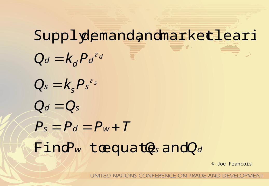
QQP
TPPP
PkQ
PkQ
s
d
and equate to Find
clearingmarket and demand,Supply,
© Joe Francois

Use ‘Solver’ in Excel to obtain numerical solution. Specified one cell as objective to be solved given constraints.
© Joe Francois
q
x1
x2
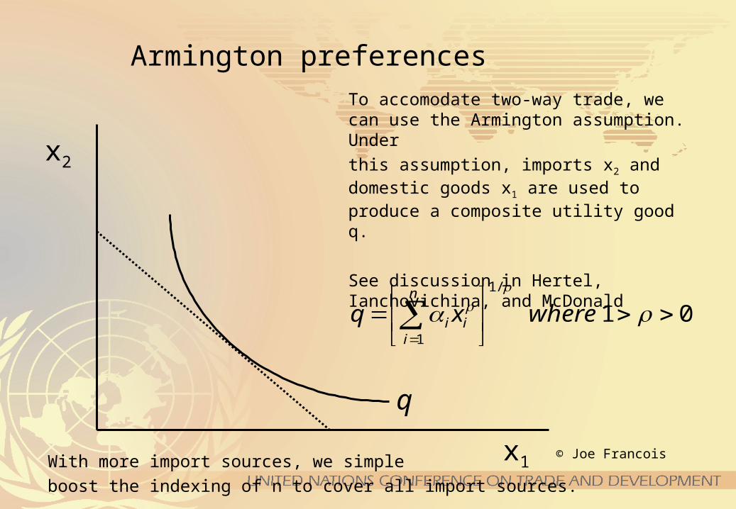
Armington preferencesTo accomodate two-way trade, we can use the Armington assumption. Under this assumption, imports x2 and domestic goods x1 are used to produce a composite utility good q.
See discussion in Hertel, Ianchovichina, and McDonald
01/1
1
wherexqn
iii
With more import sources, we simpleboost the indexing of n to cover all import sources.
© Joe Francois

Inputs
• Tariffs
• Elasticities
• World price
• Production
• Consumption
• Exports
• Imports

Output
• Consumer surplus
• Producer surplus
• Tariff revenue
• Quota rents
• Welfare
• Prices
• Production
• Consumption
• Exports
• Imports

Set up models
• Determine policy issue• Choose model• Choose country aggregation• Specify commodity/ies

Data
• Get bilateral trade and tariffs data from WITS• Other policy variables, domestic support, tariff
rate quotas, production quotas• Production data, from FAOSTAT for
agricultural products, GTAP, national accounts• Elasticities, (and cross-elasticities, Armington),
from ATPSM, GTAP, other• Check P+M=C+X, ΣM=0.

Shocks
• Common source of differences in results• Compare bound vs applied rates• Negotiate bound, but shock applied• Exemptions
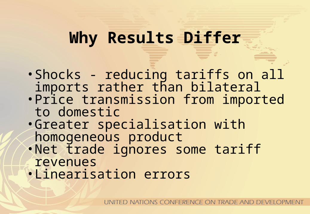
Why Results Differ
• Shocks - reducing tariffs on all imports rather than bilateral
• Price transmission from imported to domestic
• Greater specialisation with homogeneous product
• Net trade ignores some tariff revenues• Linearisation errors

Interpreting Results
• Did simulation solve? Check ΣM=0, ΣToT=0
• Check shocks are correct• Any variables below 0, i.e. <-100%?• Small trade shares problem – no change
from zero trade• Explain counter-intuitive results• Usually composition effects• Confabulation

Sensitivity analysis
• Which variables or parameters drive the results? (Armington elasticities?)
• Is there uncertainty about these variables?• Run model with different values to check
results are robust

Selling your results
• Don’t oversell (others will do this for you)• Use results to provide insights, not answers• But are results driven by assumptions –
elasticities, closures, market structure, short vs long run?

Are the negotiators correct?
• UNCTAD modelling shows some counter-intuitive results:
– EU export subsidies benefit developing countries– Tariff revenues may rise from tariff reductions,
and generally fall by less than the tariff cut– More countries lose than gain from multilateral
agricultural liberalisation– Market expansion offsets preference erosion

Summary
• Build you own for useful insights• Consider would additional complexity
(dynamics, IRTS) reverse policy implications
• Keep it simple

The End

Algebra: from first order conditionsFor CES demands (see solution sheet)
i
n
iii
NAA
i
isi
i
i
j
jsj
j
j
PEP
unknownsandequationsn
PP
EPk
it
PkEP
P
njt
PkEP
P
si
sj
,,
2
0
0
10)1(
..20)1(
/11
1
1
1
1
1
P is a composite pricePj is the price of good j
E is total expenditureksi is a supply function constant term
ka is a composite demand constant term
is the elasticity of substitution=(-1)/

GSIM
ˆ M i,r ˆ X i,r EX (i,r)ˆ P i,r* N( i,v ),(r,r )
ˆ P (i,v ),r
v
N(i,v ),(r,s)ˆ P ( i,v ),s
sr
v
N( i,v ),(r,r )[Pr * ˆ T ( i,v ),r ]v
N(i,v ),(r,s)[ ˆ P s * ˆ T (i,v ),s]sr
v
In the GSIM model, linearized Armington demand isadded up across all markets, yielding one market clearing condition for each exporter. Hence, with 10 regions and 100 potential trade flows, the model is reduced to 10 equations. See Francois and Hall 2002.
© Joe Francois