Do Entrepreneurship and Self-Employment Respond toSimpler Fiscal Incentives? Evidence from France.∗

Philippe Aghion Ufuk Akcigit(College de France, LSE, CEPR, and NBER) (University of Chicago, CEPR, and NBER)

Matthieu Lequien Stefanie Stantcheva(Banque de France) (Harvard, CEPR, and NBER)

March 20, 2017

Abstract

In this paper we use French income tax returns since 1994 to study the effects of fiscal incentivesfor self-employment and entrepreneurship. France is a good quasi-laboratory because of its uniquevariety of fiscal “regimes” for self-employment, which differ according to their financial incentives,their degrees of administrative simplicity, and the scope for misreporting income that they offer.Eligibility for the two simplified fiscal regimes, which have a low administrative burden, requiresbusiness revenues to remain below a given threshold. We show that a reform that expanded el-igibility for a simplified regime led to an immediate switch of agents from other regimes, but nooverall growth in self-employment. On the other hand, a reform which created a regime with moreadministrative simplicity led progressively to new entry by smaller than average businesses. Theeligibility thresholds create a special type of “notches” around which we observe significant bunch-ing. The thresholds have moved a lot over time, and the bunching mass has moved with them,although progressively so, and faster when the threshold change was larger. We use the measuredempirical bunching to estimate the value of administrative simplicity, a real income elasticity, anda misreporting elasticity. To do so, we exploit the many variations in policy parameters over timeand their heterogeneous impacts on agents in different tax brackets and activity types. We find thatthere is a significant misreporting elasticity and a value for simplicity, without which the observedbunching is hard to rationalize.

(JEL H21)

Keywords: Self-employment, Taxation, Entrepreneurship.

∗Aghion: College de France, London School of Economics and CEPR (e-mail: p.aghion@lse.ac.uk). Ak-cigit: University of Chicago, NBER, and CEPR (e-mail: uakcigit@uchicago.edu); Lequien: Banque de France(email: Matthieu.LEQUIEN@banque-france.fr), Stantcheva: Harvard University, NBER, and CEPR (e-mail:sstantcheva@fas.harvard.edu). Stantcheva’s work is supported by the National Science Foundation under Grant CA-REER No.1654517. Aghion acknowledges support from an Idex grant from Paris-Sciences-et-Lettres (PSL) and by apublic grant overseen by the French National Research Agency (ANR) as part of the “Investissements d’Avenir” program(reference: ANR-10-EQPX-17 - Centre d’acces securise aux donnees– CASD). We thank Simon Bunel, Francois-XavierLadant, and Cyril Verluise for outstanding research assistance.

1 Introduction

Many policies and fiscal incentives target self-employed entrepreneurs in an attempt to improve pro-

ductivity. New developments in the labor market have put self-employment at the forefront of the

policy debate again. The development of platforms such as Uber or Air BnB, and services such as

Task Rabbit or Handy challenge traditional divides between employment and self-employment. In

recent work, Katz and Krueger (2016) cast light on the rise of alternative work arrangements, the

fragmentation of the labor market, and their important implications for inequality. In Europe, these

developments have been intentionally slowed down by stricter labor regulations, at the same time as

many policies to stimulate self-employment and entrepreneurship have been implemented.

Key questions for these policies are, first, what and how strong effects they have on entry into

self-employment and on self-employed incomes. Second, are the effects mostly due to real economic

reactions, or rather to changes in the reporting of income? Indeed, the self-employed may be a set of

agents that is especially able to misreport their incomes. Do financial incentives matter most or are

simpler administrative requirements key?

In this paper, we try to answer these questions, making use of individual tax returns data from

the French internal revenue service over the period 1994-2012. France is a particularly well-suited

quasi laboratory to study self-employment because it has a very unique variety of fiscal “regimes”

or modes of taxation of self-employment, which differ according to not only the financial incentives

they provide, but also, importantly, according to their degrees of administrative simplicity1 and the

scope for misreporting income that they offer.2 These fiscal regimes have changed a lot over time and

impact different agents differently, providing valuable policy variation to study their impact on self

employment.

In Section 2, we start by describing the landscape of self-employment policies in France. There are

three regimes under which a self-employed may choose to operate, which differ along the aforementioned

dimensions. To summarize very briefly, the standard regime treats an individuals’ net business income

(revenues minus costs) as taxable income and comes with the most involved accounting requirements,

which limit the scope for misreporting and also increase administrative complexity.3 The simplified

regime, as its name indicates, simplifies administrative requirements, and uses as a taxable income

measure the gross revenues times a rebate that depends on the type of activity.4 The super simplified

regime further simplifies the administrative requirements by replacing the social security contributions

and income taxes by a unique payment proportional to the individual’s gross revenue. Both the

simplified and super simplified regimes require that revenues remain below a certain eligibility threshold

1In fact, fostering simplicity was one of the key political motivations for the reforms we will describe.2More precisely, these differences lie in the taxable income base, their tax rate, administrative and registration re-

quirements, social security contributions and VAT payments.3In the data, agents in the standard regime are mostly members of so-called Certified Accounting Centers (CACs)

which ensure sound fiscal conduct and limit misreporting.4Activity types for tax purposes are Industrial and Commercial Services, Industrial and Commercial Retail, or Non

Commercial.

1

that varies with the type of activity. Thus, broadly speaking, the simplified and super simplified regimes

are well suited to agents with small and slow-growing activities, with relatively low production costs and

investments (since the latter cannot be deducted), and who care a lot about administrative simplicity.

In Section 3 we provide key summary statistics on the self-employed for the period 1994-2012, based

on the tax returns data. The self-employed are on average much older, more likely to be retired, and

have more capital income. Women are much more represented in the Non Commercial activities. The

fraction of agents with self-employed income has remained stable at around 5% of all tax filers aged

18-65 and the fraction of those who earn only self employed income has remained at around 4% for

most of the period. Both shares have experienced a sharp rise since 2009, especially the share of those

combining self employed income with additional income.

We then provide event studies of two key reforms to fiscal incentives. The 1999 reform multiplied the

eligibility threshold for the Simplified Regime by five for Retail activities and by almost two for Services

and Non Commercial activities. This reform thus expanded the financial incentives to a larger group

of people, but did not modify the simplicity of the system. The reform led to entry into the simplified

regime and a growth in the average size of businesses in that regime. These effects of the reform were

immediate: the incentives were sufficiently large to cause a sharp and fast response, which almost

entirely took place in the very first year. There was, however, no effect on overall self-employment, as

agents simply switched from other regimes. The 2008 reform created the super simplified regime, thus

further increasing administrative simplicity and decreasing the costs of entry into self-employment.

It led to new entry by smaller than average businesses, who selected into the newly created regime,

and thus to an overall increase in self-employment. The effects were progressive, presumably because

agents needed time to adjust to or learn about the new regime.

In Section 4, we build a simple model of self-employed behavior, where the various regimes differ

– as is the case in the data– in their financial payoffs, hassle costs (i.e., the costs imposed by a lack

of administrative simplicity), and the opportunities they offer for misreporting income. In the model,

the simplified and super simplified regimes are thus less costly in terms of administrative requirements

and allow agents to misreport their income. We show that the choice of regime agents make is roughly

in line with what the model’s optimization predicts, given their income, tax bracket, and activity type

(which determines the generosity of the simplified and super simplified regimes).

The eligibility thresholds create a special type of discontinuity, so-called tax “notches.” These are

studied in a rich empirical literature on the effects of taxation on taxable income using the “bunching”

methods, as surveyed in Kleven (2016). Key papers are Saez (2010), Chetty et al. (2011), and Kleven

and Waseem (2013). Our setting is well-suited to such a bunching analysis given the strong discon-

tinuities created by the eligibility thresholds and their many movements over time, which eases the

identification. Our analysis differs from standard bunching analyses in two key ways: at the threshold,

there is not only the average tax rate that changes, but also the administrative simplicity and the

ability to misreport income. Second, at the threshold, there is a lot of heterogeneity across agents in

terms of their tax brackets (and, hence, the effective payoff from bunching) thanks to the peculiarities

2

of the French tax system and in their benefit from remaining in the simplified regimes because of

different activity types (and the different rebates they entail).

We show that there are discontinuous jumps around the eligibility thresholds in the proportion

of agents who are in the simplified and super simplified regimes. Most importantly, in the income

distribution of self employed income, there are large and significant excess masses right before the

thresholds of eligibility. The thresholds have changed a lot over time and the excess mass follows

the thresholds’ movement, fostering confidence in the fact that the excess mass is indeed caused by

the latter. Agents in higher tax brackets, who have more to gain from optimizing their self-employed

regime, exhibit stronger bunching behavior.

We study the dynamic adjustment to the changes in thresholds over time and find that, first, when

the threshold changes by a little, there is a smaller bunching at the new threshold, which grows over

time, and also a remaining bunching at the old, no longer applicable threshold. When the threshold

remains stable over time, there is a progressive increase in bunching. Large changes in the threshold

lead to immediate large bunching at the new notch, which keeps growing over time. These findings are

consistent with either a model where salience and rational inattention play a role, so that agents do

not learn about small changes, but do learn about large changes, or with a model in which there is a

fixed cost of adjusting one’s activity, which is only worth incurring if the policy change is large enough.

In any case, there can be both real and avoidance responses, although the large number of agents who

report income exactly at the kink is striking and casts some doubt on the real response hypothesis.

In Section 5, we use the measured empirical bunching magnitudes to estimate the value of ad-

ministrative simplicity and two elasticities: an elasticity of real income responses and a misreporting

elasticity. A key advantage for this estimation is that there is a lot of variation in the policy param-

eters over time and a lot of heterogeneity across agents in terms of their tax brackets, activity types,

and self-employed income that allows for many informative data moments.5 We find that there is a

significant misreporting elasticity and a value for simplicity, without which it is difficult to rationalize

the observed bunching at the threshold.

Our paper is related to several studies on the effects of taxation on entrepreneurship and self-

employment. Cullen and Gordon (2007) use U.S. tax returns data and show that different components

of the tax system, such as the progressivity and the marginal tax rates, have had distinct and significant

impacts on entrepreneurial risk-taking (see also Cullen and Gordon (2006)). Gentry and Hubbard

(2000) find that a progressive tax system discourages entry into entrepreneurship. Bruce (2000) finds

using the Panel Study of Income Dynamics that reducing marginal tax rates on self-employed income

reduces the probability of entry into self-employment, while reducing the average tax rate slightly

increases entry. We do not study the effects of general income taxation, but specific fiscal incentives

for the self-employed, which modify both the financial returns to and the simplicity of self-employment.6

5Our strategy is thus related to other papers who use empirical bunching magnitudes to estimate a structural model,such as Einav et al. (2017).

6In fact, new entry into self-employment seems to have occurred only when the system was hugely simplified as throughthe 2008 reform.

3

More generally, our work is also related to papers on the determinants of entrepreneurship (see,

among others, Hamilton (2000), Schoar (2010), Adelino, Schoar and Severino (2015), and Schmalz,

Sraer, and Thesmar (2016)), and we focus specifically on the role of fiscal incentives, taxation, and

administrative simplicity.

A recent series of papers uses the bunching methodology to study a range of different topics such

as intertemporal allocation in response to mortgage contracts changes (Best et al., 2015), transaction

taxes in housing markets (Best and Kleven, 2016), corporate taxation (Best et al., 2015), responses to

the EITC (Chetty et al., 2013), and the social security earnings test (Gelber et al., 2014). The novel

French tax data is also used in two important contemporaneous papers that study income distributions

and wealth distributions in France by Garbinti et al. (2017) and Garbinti et al. (2016). Our focus is

complementary by studying self-employed individuals.

2 The Landscape of Self-Employment in France 1994-2012

In this Section, we describe the landscape of self-employment in France over the period 1994 to 2012,

by providing details on the institutional background in France, the different fiscal incentives in place,

and their evolution over time.

2.1 A Primer on the French Personal Income Tax System

We start with a brief note on the French tax system with regards to the features that will be relevant

for the self-employed. Taxable income of a household is the sum of all the sources of income minus

deductions (itemized and standard) and the taxable income from self-employed activities. Each house-

hold has a scaling factor called the number of parts, which is determined by the household composition.

For a single adult, that scaling factor is one, for a married couple, it is 2. Each child adds 0.5, up to

the third child which adds 1. In addition, a disabled child adds 0.5. For example, a married couple

with a child has a number of parts equals to 2.5. A married couple with 3 children has a number of

parts equals to 4, and a married couple with one disabled child has a number of parts equals to 3.

The tax bracket is determined by the family coefficient, defined as taxable income divided by the

number of parts. Once this tax rate is determined, the household owes the tax rate times the full

taxable income.7 Appendix A.1 provides the formal details of how tax brackets are determined..

An important feature of the tax system it thus that there is not a unique map from income to tax

bracket, which means that at a given taxable income, there are several possible tax brackets based

on family structure. In fact, at a given taxable income, there can be a wide range of tax brackets

represented, which will be helpful in our analysis and for the estimation.

The national income tax schedule is shown for illustration for the years 1994, 2006, and 2012 in

Figure 1. The tax schedule changes almost every year as part of the yearly budget voted by the French

7There is a complication due to the fact that the number of parts cannot grant the household more tax reduction inabsolute terms than a threshold, but it can be ignored for our purposes.

4

Table 1: Summary of the self-employed regimes

Regime (1) Standard (2) Simplified (3) Super simplified

Taxable base Net business income Gross revenues × (1- rebate) Gross revenues

Tax rate Income tax rate Income tax rate Flat rate

Registration Standard Standard Simplified

Accounting requirements Detailed Only for audit Only for audit

SS contributions Standard Standard rate Flat rate

but levied on taxable base levied on gross revenuesSubject to VAT Yes No No

Timing of payments Annual Annual Monthly or quarterly

Notes: The eligibility thresholds for each of these regimes are (as of 2012): 32,600 euros for the Services and NonCommercial and 81,500 euros for the Retail activities. Certain types of activities are excluded from the simplified regime(those are most notably agricultural activities, leasing of durables and equipment, leasing of professional or non furnishedbuildings, and real estate businesses) and from the super simplified regime (those are, in addition to the aforementionedones, liberal professions such as lawyers, doctors, insurance agents, or accounting experts, and formally registered artistsrewarded through copyright). Revenues cannot be negative and thus, no deficit can be claimed in the simplified andsuper simplified regimes. In the super simplified regime, the flat rate is due even if the agent is in the zero personalincome tax bracket. However, if gross revenues are zero, no payments are made (either for the income tax or for thesocial security contributions). In the simplified regime, if gross revenues are zero, no payments are made for the incometax, but a minimal payment is still due for social security contributions.

Parliament.8

2.2 Self-employed Regimes and Fiscal Incentives in France

2.2.1 Three main regimes:

An individual who owns a business and is self-employed can select to remain in the personal income

tax code or to be subject to the corporate tax code. The latter is the only choice available to large

businesses, but typically not used for personal, self-employed activities which are the focus of this

paper.

As of 2012, the self employed individuals in France who wanted to remain in the realm of personal

income taxation could be in one of three regimes. These regimes can be characterized along seven

dimensions summarized in Table 1: i) the taxable income base, ii) the tax rate, iii) the registration and

startup requirements, iv) the accounting and reporting requirements, v) the mode of social security

contributions, vi) the mode of VAT payments, and vii) the timing of payments. In all regimes, the

requirements for professional qualifications and the quality and safety standards of each activity are

identical.

8Called the Projet de loi de Finance.

5

(1) The standard regime:9

All self-employed are eligible for the standard regime. The taxable base is the business’ net income,

i.e., the difference between gross revenues and costs, including depreciation of assets and investments

according to standard accounting rules. This taxable income is simply added to an entrepreneur’s

household income and taxed at the entrepreneur’s income tax rate (which, naturally, depends on his

tax bracket). The registration procedure for starting an activity is standard. Tax payments occur at

the normal tax filing date and social security payments happen separately through the regular social

security procedure. Activities are subject to the VAT and can charge VAT on their products sold and

claim VAT on their inputs. In addition, self-employed in this regime can benefit from tax credits, such

as those for R&D spending.10 and some government help in special zones, none of which is available

when filing under one of the simplified regimes.11 Finally, businesses in this regime can join a certified

accounting center (hereafter, CAC), which helps them keep and check their accounts and serves as

a garant of sound fiscal conduct to the tax authority. Joining such a center confers benefits, most

notable escaping the 25% augmentation of the taxable income base12 that faces business that do not

join.13 We discuss these CAC in detail below. The key advantage of this regime is thus that it allows

the individual to subtract its input and running costs from its taxable income. The main cost is that

it entails more stringent administrative, accounting, and reporting requirements.

(2) The simplified regime :14

To qualify for the simplified regime, an entrepreneur’s income must be below a pre-specified thresh-

old, which varies with the type of activity and has changed a lot over time; the solid lines in Figure 2

show the evolution over time of the thresholds respectively for the Industrial and Commercial activi-

ties, the Industrial and Commercial Retail activities, the Industrial and Commercial Services, and for

non commercial activities. These thresholds are not very high for the Services and Non commercial

activities (equal to 32,600 euros in 2012), but much higher for the Retail activities (81,500 euros).

Taxable income is calculated as revenues times a scaling factor 1−µ, where the rebate µ is determined

by the tax administration, which depends on the activity type and has changed over time. The dotted

lines in Figure 2 show the evolution over time of the rebate rates for the different types of activities.

This taxable income is added to the rest of an agent’s income and taxed at his regular income tax rate.

Social security contributions are also determined on this same income base (revenues times 1− µ), at

9“Regime Reel.”10E.g., Credit d’impot recherche or the credit d’impot competitivite et emploi.11Zones geographiques prioritaires ZRR, AFR, BER, QPV.12I.e., those businesses pay a tax on 125% of their normal taxable income.13“Centre de Gestion Agrege”14We lump together under this heading two regimes, which are indistinguishable in the tax data: the (1) Regime

Micro-entreprise and the (2) Regime Auto-Entrepreneur sans Option Liberatoire, i.e., the super simplified regime belowwithout the flat rate option. Those two regimes differ in their social security contributions: in (1), a minimal amount ofsocial contributions is due even there are zero revenues, in (2) a flat rate applies to all revenues (rather than revenuesminus rebate), but on average the effective rate on revenue is similar. There are also minor differences in the registrationand start-up modalities, which streamlined further in the super simplified regime. These two regimes are entirely identicalfor tax purposes and hence impossible to differentiate in the tax returns. We will henceforth ignore this distinction.

6

the regular social security rates. If revenues are zero, no income tax is owed, but a minimal social

security contribution is nevertheless due. Registration and start-up requirements, the timing of tax

and social security payments are similar as for the standard regime.

There is no application of the VAT for this regime: thus entrepreneurs in the simplified regimes can

neither charge VAT to their customers, nor claim VAT on their inputs. Thus the main advantage of

this regime is the rebate on the taxable income, which may, for some self employed, be more generous

than their actual costs. In addition, all procedures are simplified. It does, however, impose revenue

threshold restrictions. which are not well-suited to larger scale activities. One thing to note is that,

despite the fact that taxable income is determined as a fraction of revenues, self-employed in this

regime are nevertheless required to keep accounts for their activity with receipts from purchases and

sales linked to the activity in case there is an audit.

(3) The super simplified or “Flat rate” regime:15: The super simplified regime has similar rules

to the simplified regime, but increases administrative simplicity even further. The taxable income base

is total gross revenues (i.e., the rebate µ is zero) and the tax rate is a flat rate that, once paid, frees

the agents from both income tax and the social security contributions due. The flat rate differs by

activity and has also changed over time. Income tax and social security payments are due monthly or

quarterly, based on actual realized revenues (cash in hand), and are all taken care of at the same time,

thus minimizing filing and administrative hassle (however, potentially deterring agents with credit

constraints). The flat rate paid is completely unrelated to an agent’s actual income tax bracket or

tax rate.16 Thus, even a household which is in the zero income tax bracket still owes the flat rate

times revenue payment in this regime. An agent owes no income tax or social security payments if

his revenues are zero, but can also not claim any deficits he may have. Registration and start-up

modalities are further simplified. To be eligible for this regime, the same threshold requirements on

revenues as for the simplified regime apply, but, in addition, the family coefficient in fiscal year t− 2,

has to be below the upper bound of the third tax bracket in year t − 2.17 For instance, that upper

bound was 26,420 euros for year 2010, so that for households to be eligible for the super simplified

regime in 2012, their family coefficient in 2010 had to be lower than 26,420 euros.

Thresholds, eligibility, and grace period:

In the simplified and super simplified regimes, if the agent’s revenues end up being higher than

the threshold, there is a two-year grace period, as long as the revenues are still below a “tolerance

threshold” (which is, e.g., 6.1% higher than the actual threshold in 2012 for the Services and Non

Commercial Activities and 9,9% higher for the Retail Activities).18 If the threshold is crossed for more

15Regime Auto-Entrepreneur avec Option Liberatoire”16A subtlety to note is that, to determine the overall tax bracket of the household, it is the revenues times 1−µ where

µ is the same rebate as in the simplified regime above that is added to the rest of a household’s income. It is not the fullamount of revenues that is added, which would make the super simplified regime very unattractive.

17Recall that the family coefficient is, as explained above is equal to taxable income divided by the number of householdparts.

18This grace period and tolerance threshold do not apply in the first year after the business’ creation.

7

than two years or if the tolerance threshold is crossed, the special regime status is lost, and the agent

has to file under the standard regime.

Choosing a regime for each fiscal year:

There are some key considerations when it comes to deciding which regime to be in.

First, agents have to decide by the month of February of fiscal year t which regime they want to be

affiliated with for their income during fiscal year t. This means that agents make this choice based on

their expected – rather than actual– revenues, costs, and business growth. This may also potentially

increase the incentives to misreport income ex post if it turns out that revenues were higher than

expected.

Based on these differences, we can imagine that, broadly speaking, agents who should chose the

standard regime are those with high business running costs, with larger investments (since no invest-

ment can be deducted or depreciated in the other regimes), who want to hire employees, whose activity

is expected to grow rapidly during the year, who may expect the need to claim a deficit, and who do

not find the extra administrative requirements particularly costly. Conditional on having a given cost,

investment, and overall business structure, it is agents in higher tax brackets who would face the

strongest incentives to optimize their regime.

It is also worth mentioning that inertia and “default options” could be playing a more behavioral role

in the regime choice. As is clear from our description, the regime rules are somewhat intricate, and the

thresholds and rates have changed extensively over time, which implies potentially high attention and

learning costs from switching regimes. Agents may thus prefer – once the fixed cost of understanding

a regime having been incurred – to stay put as long as their financial loss from not switching is small

enough. In addition, as regards the super simplified regime, this is an option that agents have to

actively pursue when they register their business for the first time, or each fiscal year – it is a box that

has to be actively checked on the form. The default is to remain in the simplified regime.

2.2.2 Activity types:

For tax purposes, the self-employed are classified into three types of activities: (i) the “Industrial and

Commercial Services” category, referred to as “I&C Services” below,19 (ii) the “Industrial and Com-

mercial Retail” category, referred to as “I&C Retail,”20 and the (iii) the Non-commercial category.21.

These activity types, defined for fiscal purpose, do not necessarily align well with the underlying

economic characteristics of businesses. For instance, developing and selling software pertains to the

Non-commercial type, while purchasing and selling equipment goods pertains to the I&C Retail cate-

gory. Similarly, bakery, butchery, or restaurant businesses are counted as I&C Retail activities, while

construction work, plumbery, carpenters, and auto or other repair shops and dry cleaning count as

19These are the so-called “Benefices Industriels et Commerciaux Services”.20“Benefices Industriels et Commerciaux Vente”21“Benefices Non Commerciaux”

8

I&C services. Moreover, all professional activities, such as those done by consultants, private coaches,

translators, or experts belong to the Non Commercial category.

2.2.3 Certified accounting centers

As noted above, agents in the standard regime who are members of a certified accounting center (CAC)

do not have to pay taxes on an extra 25% top-up of their taxable income that faces non-members.

It would thus seem that all agents in the standard regime should adhere to a CAC. In fact, a large

proportion do. Figure 3 shows that at higher income levels, almost 100% of all agents in the standard

regime are CAC members. Why is it the case that at lower income levels, there is a gap? First of

all, agents in the zero tax brackets in the standard regime face a zero tax rate and, unless the extra

25% tax makes their taxable income cross the first tax bracket threshold, their taxes are not increased

from not being members. However, even taking out those agents in the zero tax bracket, the fraction

of those who adheres at low income levels is still pretty low. What can explain this discrepancy is that

adhering to a CAC makes it harder to misreport income and engage in tax avoidance – one of they

key reasons for CACs to exist in the first place. If an agent plans to misreport more than 25% of their

taxable income and are not averse to the risk of being audited, it may be beneficial to remain a non

CAC member.

The Cour des Comptes (2014) reports that conditional on an audit, the size of the penalties among

non-CAC members is larger than among CAC members (around 26,000 euros versus 7,000 euros).22 In

addition, the Cour des Comptes (2014) states that the discrepancies in taxes due and taxes actually

paid among CAC members seems mostly due to genuine accounting mistakes and delays in payments,

and almost never to tax evasion motivations, as opposed to the discrepancies noticed among non-CAC

members.

The large fraction of agents in the standard regime who are members of a CAC, especially around the

threshold that we will focus on (where it is essentially 100%) lends support to the modeling hypothesis

we will make below, that cheating is much easier in the simplified or super simplified regimes and much

more difficult in the standard regime.

2.3 History and Key Reforms

The thresholds and rates applicable to each regime have changed extensively over time as shown in

Figure 2. Nevertheless, two major reforms stand out:

The 1999 reform The 1999 reform focused on the simplified regime, for which it greatly extended the

threshold from 100,000 French Francs (15,244 euros) to 500,000 French Francs (76,220 euros) before

tax for I&C Retail businesses and to 175,000 French Francs (26,678 euros) before tax for the I&C

Services or Non Commercial activities. Moreover, rebates on VAT tax payments become applicable

22Penalties are strongly positively correlated with the amount misreported.

9

top all individuals under the simplified regime and whose income falls below the new thresholds (500000

Francs and 175000 Francs). In a nutshell, the 1999 reform multiplied the eligibility threshold for the

simplified regime by five for I&C Retail and by almost two for I&C Services and Non Commercial

activities. Before 1999, the thresholds were so low as to only be applicable for very small activities and

the simplified regime was not a relevant option for many self-employed. We will see below that this

reform had large extensive margin effects, with many self-employed entering the simplified regime.

The 2008 reform The 2008 reform created the super simplified regime, out of the desire to further

streamline the simplified regime. Indeed, the key motivation was to further save on administrative costs

by replacing the social security contributions and income taxes by a unique tax transfer proportional

to the individual’s revenue.

The administrative procedure for moving from the simplified regime to the super simplified regime

following the 2008 reform, is rather light: all that is required is for the individual to fill a form by

December 31st of year t− 1 to qualify for entry into the super simplified regime in year t.23

3 Data, Descriptive Statistics, and the Effects of the Key Reforms

In this Section, we provide summary statistics on the demographic characteristics, incomes, and num-

bers of the self-employed over time, especially as compared to wage earners. We also provide an event

study of the effects of the main 1999 and 2008 reforms.

3.1 Data

We use tax returns data from the French Internal Revenue Service24 over the period 1994-2012. For

all years, we have the full tax return information on a representative sample of 500,000 households

(out of around 33 million on average per year over that period). Each has an associated weight that

corresponds to its relative importance in the overall household population in terms of income level and

demographic characteristics (marital status, number of children, income, etc..). For the year 2011, we

have access to information on the whole population, which comprises about 36 million households.25

The income and demographic information on each household is captured by around 3000 variables.

In particular: (i) the demographic data tell us about the age of the tax filer, the number of children

in her household, family situation, whether the tax filer is active or unemployed or retired, her fiscal

geographic location; (ii) the income data tell us about the household’s income for each activity that

household members are involved in, whether the income is a from salaried or non-salaried work, and

23Exceptionally in 2009 (the year when the super simplified regime was introduced) individuals were granted extra timeuntil March 31st of year t.

24Direction Generale des Finances Publiques (DGFiP)25While this is still work in progress, subsequent versions of this draft will replace the samples for all years between

2002-2014 with full population data.

10

about all capital income.26

3.2 Descriptive Statistics on Income and Demographics of the Self-Employed

We now turn to summary statistics from the new datasets to document the demographic characteristics,

incomes, and evolution of self-employed in France.

Figure 4 shows the evolution over time of the fraction of self-employed among the total population

aged 18 to 65. We distinguish people according to whether they have any self-employed income (the red

line) and whether they have only self-employed income (the blue line). The fraction of self employed

has remained stable over time, at around 5%, while the fraction with only self-employed income has

been very slightly decreasing from 4.2% in 1994 to 3.7% in 2009. But self-employment has seen a rise

since 2009, especially in the number who have some, but not only, self-employed income. In 2012 the

fraction with any self-employed income had risen to 6%. The two vertical red lines represent the 1999

and the 2008 reforms respectively, which we will study in detail below.

Table 7 shows the demographic characteristics (in Panel A), income (in Panel B) and income tax

information (in Panel C) of the self-employed and wage earners, as well as their numbers (in Panel D)

over the whole period 1994-2012. The sample is split into three subgroups, which are: (i) wage earners

only, (ii) self-employed only, (iii) have any self-employed income.

The table shows that the self-employed tend to be older on average 8-9 years older than wage earners

and are almost three times as likely to be retired. This goes against the preconceived idea whereby

the self-employed – in this vision considered to be “entrepreneurs”– are the young. The “unemployed”

variable refers to the fraction who have perceived any unemployment benefits during the year. Agents

in this table are, by definition, employed or earning self-employed income for at least part of the year.

The self-employed are less likely than the wage earners to have received any unemployment benefits.

Panel B shows that those who receive self-employed income only earn on average around 33,000

euros. Those who earn some, but not exclusively, self-employed income have on average 30,000 euros

of self-employed income and very little wage income, around 6,000 euros. Self-employed agents have

more than three times more capital income that wage earners: around 6,000 as compared to 1,900.

Panel C shows the distribution across tax brackets of each group. Self-employed individuals are

more than three times more represented in the highest tax brackets, and disproportionately less in the

second lowest one.

Tables 8, 9 and 10 reproduces Table 7 for different groups of years. There are several noteworthy

facts. First, while wage income has on average been consistently rising (adjusted for inflation), average

self-employed income experienced a fall post 2008. This is despite and at the same time as the number of

agents with self-employed income rose as shown in Figure 4. We will return to this in more detail below

when we study the 2008 reform that introduced the super simplified regime. Second, capital income

increased strongly for all groups. Third, the proportion of self-employed who perceive unemployment

26Using the year 2011 for which we have both the subsample of 500,000 and the full population data, we can indeedcheck that all results look very similar when we use either the full sample or the subsample.

11

benefits at some point during the year doubled from the 1999-2008 to the 2009-2012 period, while the

number for wage earners or for the population as a whole only increased by 50%.

3.2.1 Comparing Industrial and Commerical and Non Commercial Activities:

Table 11 shows the demographic and socioeconomic variables for the self-employed split by activity

type. There is a strong gender gap, with women being much more represented in the Non Commercial

activities. Maybe as a result of this, the average number of children and the likelihood of having

children is higher in the Non Commercial activities. Retired people are much more represented in I&C

Retail and I&C Services. Earnings are much larger in Non Commercial activities – including wage

income, and as a result, the tax bracket distribution is shifted to the right relative to the Industrial

and Commercial self-employed. There is an almost double number of individuals with Industrial and

Commercial income.

3.2.2 Tax brackets and regimes

Figure 5 shows for each regime the fraction of individuals in each tax bracket. Panel A (resp. Panel B

and Panel C) in Figure 5, shows the fraction of individuals in the standard regime (resp. the simplified

regime and the Super simplified regime) in each tax bracket. In each of the three Panels, the green

curve corresponds to the fraction of individuals in the first income bracket, the orange curve depicts

the fraction of individuals in the second income bracket, and the sienna color and blue color curves

depict the fraction of individuals in the third and fourth income brackets respectively.

In particular, when comparing between the three panels, we see that individuals in the standard

regime are much more likely in the top brackets than the other two groups of individuals (in the

simplified and super simplified regimes), and that most of the individuals in the super simplified

regime (the French ”Auto-Entrepreneurs”) lie in the lower income brackets.

3.3 Effects of the Reforms to Self-Employment Statuses

We now turn to studying in more detail the extensive and intensive margin responses that occurred

after the two large reforms in 1999 and 2008.

3.3.1 The 1999 reform

In a nutshell, the 1999 reform multiplied the eligibility threshold for the simplified regime by five for

I&C Retail activities and by almost two for I&C Services and Non Commercial activities. As could

be expected, this reform resulted in mass entry into the simplified regime, whose thresholds were

previously too restrictive for any more than tiny self-employed activity.

Figure 6 shows the effects of this 1999 reform. Panel (a) considers the number of agents in the

standard and in the simplified regime, as well all self-employed (“All”). The numbers are normalized at

12

100 in 1994. There is a sharp increase in the number of agents in the simplified regime in 1999. There

is a sharp corresponding decline in the number of agents in the standard regime. It thus seems that the

threshold limit was very constraining pre 1999 and that there was a very significant 60% increase in

the number of agents in the simplified regime after the expansion. There is a very modest increase in

the overall number of self-employed (the base is larger, and hence the proportional increase is smaller).

Hence, the effect of the reform was to make individuals switch from one regime (the standard one) to

another (the simplified) when the latter was made more generous, rather than to simulate new entry

into self-employment.

Panel (b) shows the mean revenues earned per business in each of the regimes. While all regimes

experienced some growth in mean income, businesses in the simplified regime expanded their incomes

most. This in turn may reflect both, an extensive margin effect whereby high-income individuals enter

the simplified regime, and an intensive margin effect whereby individuals already in the simplified

regime are induced to work harder as performing well reduces less the probability of being subsequently

excluded from that regime (i.e., of crossing the eligibility threshold). Given the results from Panel (a),

it makes sense that it is on average larger businesses which made the switch from the standard to

simplified regime, i.e., those who may previously have found the simplified more attractive but were

constrained by the threshold limit.

Thus, the reform led to both entry into the simplified regime and a growth in the size of its average

business. These effects of the reform were immediate: the incentives were sufficiently large to cause

a sharp and fast response, which almost all took place in the very first year. There was, however, no

effect on overall self-employment.

3.3.2 The 2008 reform

We now turn to the 2008 reform that created the super simplified regime. Figure 7 shows the time

series around the reform of the number of self-employed and their mean revenues. Panel (a) shows that,

after the time of the reform, there was a sharp growth in simplified + super simplified entrepreneurs.

The increase seems to come most sharply from non-simplified entrepreneurs since the number of en-

trepreneurs in the simplified regime grows more marginally.27 Finally, there is actually a reduction in

the number of entrepreneurs in the standard regime, indicating a shift from one regime to the other.

On net, however, there is new entry into self-employment as can be seen from the fact that the number

of all self-employed also gradually increases post 2008, after having been stagnant in the pre-reform

period.

Panel (b) shows the mean revenues pre and post reform. The reform seems to have allowed entry

of much smaller businesses, and pushed down the average revenues per business for businesses in the

super simplified, and overall. In fact, even the simplified regime, excluding the super simplified

27The reason why we merge the simplified and the super simplified regimes in the figure, is simply that the supersimplified regime did not exist prior to the 2008 reform.

13

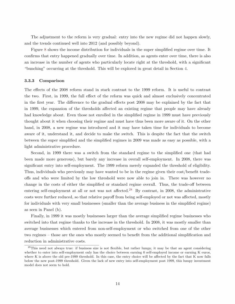
The adjustment to the reform is very gradual: entry into the new regime did not happen slowly,

and the trends continued well into 2012 (and possibly beyond).

Figure 8 shows the income distribution for individuals in the super simplified regime over time. It

confirms that entry happened gradually over time. In addition, as agents enter over time, there is also

an increase in the number of agents who particularly locate right at the threshold, with a significant

“bunching” occurring at the threshold. This will be explored in great detail in Section 4.

3.3.3 Comparison

The effects of the 2008 reform stand in stark contrast to the 1999 reform. It is useful to contrast

the two. First, in 1999, the full effect of the reform was quick and almost exclusively concentrated

in the first year. The difference to the gradual effects post 2008 may be explained by the fact that

in 1999, the expansion of the thresholds affected an existing regime that people may have already

had knowledge about. Even those not enrolled in the simplified regime in 1999 must have previously

thought about it when choosing their regime and must have thus been more aware of it. On the other

hand, in 2008, a new regime was introduced and it may have taken time for individuals to become

aware of it, understand it, and decide to make the switch. This is despite the fact that the switch

between the super simplified and the simplified regimes in 2009 was made as easy as possible, with a

light administrative procedure.

Second, in 1999 there was a switch from the standard regime to the simplified one (that had

been made more generous), but barely any increase in overall self-employment. In 2008, there was

significant entry into self-employment. The 1999 reform merely expanded the threshold of eligibility.

Thus, individuals who previously may have wanted to be in the regime given their cost/benefit trade-

offs and who were limited by the low threshold were now able to join in. There was however no

change in the costs of either the simplified or standard regime overall. Thus, the trade-off between

entering self-employment at all or not was not affected.28 By contrast, in 2008, the administrative

costs were further reduced, so that relative payoff from being self-employed or not was affected, mostly

for individuals with very small businesses (smaller than the average business in the simplified regime)

as seen in Panel (b).

Finally, in 1999 it was mostly businesses larger than the average simplified regime businesses who

switched into that regime thanks to the increase in the threshold. In 2008, it was mostly smaller than

average businesses which entered from non-self-employment or who switched from one of the other

two regimes – those are the ones who mostly seemed to benefit from the additional simplification and

reduction in administrative costs.

28This need not always true: if business size is not flexible, but rather lumpy, it may be that an agent consideringwhether to enter into self-employment only has the choice between earning 0 self-employed income or earning K euros,where K is above the old pre-1999 threshold. In this case, the entry choice will be affected by the fact that K now fallsbelow the new post-1999 threshold. Given the lack of new entry into self-employment post 1999, this lumpy investmentmodel does not seem to hold.

14

4 Model and Reduced Form Evidence

In this section, we provide reduced form evidence of behavioral responses around the thresholds, over

time, and for different regimes and agents. We first start by outlining a simple model of self-employed

behavior that provides the intuition for the reactions of agents to fiscal incentives in each regime. While

useful to frame the empirical evidence, the reduced-form results we present here are not reliant on any

model.

4.1 Model

To better understand individuals’ regime and income choices, we build the following very simple model

of self-employed behavior. Each agent has a type θ that captures his productivity and that decreases

his cost of earning a given amount of income. We use the words revenues and income interchangeably.

The disutility of earning income y for an agent of type θ is denoted by h(y, θ), increasing in y and

decreasing in θ. A given individual can operate in one of the three regimes above: the simplified

(regime “m”) the super simplified (regime “f”) and the standard one (regime “r”). Effective business

costs, taking into account inputs, VAT payments, investments and so on are modeled as a fraction ci

of gross output yi in each of the regimes i = m, f, r. An agent can misreport his true income; let yi be

reported income. The cost of doing so is g(yi − yi), increasing and convex in the difference between

true and reported income. In addition, each regime entails a hassle cost ai, reflecting the reporting,

registration, and accounting requirement costs.

An agent’s utility in regime i = m, f, r is thus:

ui = ci − h(yi, θ)− g(yi − yi)− ai

where ci is consumption.

We capture the policy parameters as follows: µ is the rebate on gross revenues in the simplified

and super simplified regimes, so that the taxable income for agents in these regimes is (1−µ) · y, with

y being revenues or income. τy is an agent’s income tax rate and τ ss the social security contributions

rate. The effective rates in each regime are denoted by τi. In the standard regime, τr is equal to the

sum of the income tax and social contribution rates, levied on net income (1− cr)yr. In the simplified

regime, τm is levied on (1− µ)ym. In the super simplified the rate is the flat rate τf that covers both

the income tax due and the social security contributions and is levied on gross income.

We make two assumptions. First, we assume that the hassle costs are low enough in the super

simplified regime, so that af = 0. Second, we assume that because of the very large adherence to the

certified accounting centers, and the difficulty of misreporting income when a CAC member, there is

no willful misreporting of income in the standard regime.

Substituting for the budget constraint under each regime, we obtain the following expressions for

15

utility as a function of policy parameters and individual choices:

um = (1− cm)ym − τm(1− µ)ym − h(ym, θ)− g(ym − ym)− am

uf = (1− cf )yf − τfyf − h(yf , θ)− g(yf − yf )

ur = (1− cr)(1− τr)yr − h(yr, θ)− ar

In the simplified and standard regimes, the tax rate is the same for any given agent, namely equal

to τ = τy + τ ss, i.e., the sum of the personal income tax rate and the social security contribution rate

(the tax base on which it is levied is, however, different in these two regimes).

In the super simplified regime, the tax rate is equal to the flat rate τf 6= τy + τ ss and µ = 0.

4.2 Regime Choice

Let us first discuss a few methodological points. First, note that the I&C Retail activities’ threshold

is placed much higher – in fact, it seems so high that the income distribution is very thin at that level

and there is not enough mass to detect bunching behavior. In this Section, we therefore only focus on

the I&C Services and Non Commercial Activities.

Second, when studying all self-employed agents jointly, we need to take into account the fact that

the self-employed in the standard regime have to report only their net income (revenues minus costs),

while those in the simplified and super simplified regimes only have to report their revenues (and

not their costs). We can, however, convert these reports into a common and comparable (reported)

“taxable” income measure: for the agents in the standard regime, taxable income is equal to net

income, while for agents in the simplified regime it is equal to revenues time the net of rebate rate,

and for those in the super simplified it is simply revenues. Similarly, we convert the thresholds for the

simplified regime into taxable income equivalent, which yields two thresholds (one for I&C Services

and one for Non Commercial activities, due to their different rebates). The thresholds for the super

simplified regime remain as such, regardless of the activity type, since there is no rebate. The taxable

incomes of agents across all regimes are now directly comparable.

Third, when we consider only agents in any simplified regime (whether simplified or super simpli-

fied), we can directly work with the reported revenues, no conversion into taxable income is needed,

and, as a result, the threshold is the same for the I&C Services, and Non Commercial activities.

4.2.1 Evidence of behavioral responses in the regime choice

We start by checking whether the proportion of agents who choose the simplified or super simplified

regimes exhibits uneven behavior around the thresholds. We use the full population data for 2011,

although the results are very similar for the other years.

Figure 9 shows the fraction of agents in any simplified regime among all self-employed, as a function

of their taxable income in 2011. The vertical lines represent the thresholds of taxable income for being

16

in the various regimes. We see that there are consistently sudden jumps in the fraction of agents in

a simplified regime at those thresholds. That the response is especially strong at the super simplified

threshold is due to the fact that that threshold applies to both I&C Services and Non Commercial

activities, and hence attracts a larger mass of people, while the other thresholds apply to one activity

type only because of the different rebate rates.

We next consider the fraction of agents who choose the super simplified regime, conditional on

choosing any simplified regime. In this case, we can directly use the reported gross revenues rather

than convert them into reported taxable income. Figure 10 shows the fraction of agents choosing the

super simplified regime at each revenue level: It again increases sharply right before the eligibility

threshold.

These discontinuities in the fraction choosing the simplified or super simplified regimes around the

eligibility thresholds is a first indication for behavioral responses to the thresholds.

4.2.2 Choice between the standard regime and any simplified regime

As explained in Section 2.2, the choice between the standard and the simplified depends on many

factors, the importance of which differs for different agents. An entrepreneur’s project, growth projec-

tions, and cost structure will affect this choice. In our model of Section 4.1, these different features

are captured by the costs cm, cf , and cr, the hassle costs am, af , and ar, and the tax bracket of the

agent, captured by τy. Given this array of factors affecting regime choice, it is hard to assess based on

observed choices whether agents are making a rational choice between the standard and the simplified

regimes.

Nevertheless, we can document how many agents pick a simplified regime, over time, at different

income levels, in different tax brackets, and for different activities. Recall that because of the way tax

brackets are determined in the French tax code, there is not a unique map from income to tax bracket,

which means that at a given taxable income, there are several possible tax brackets based on family

structure. There are two interesting predicted comparative statics to explore here.

First, when an agent’s self-employed income is higher, his tax bracket is on average higher (although

the correlation is imperfect), and he may no longer be eligible for the simplified regime; higher income

agents are more likely to be constrained by the threshold on revenues and thus unable to choose a

simplified regime. This is illustrated in Figure 11. We show here the proportion of self-employed agents

(defined as having non-negative self-employed income) who are in the simplified or super simplified

regimes, within different tax brackets. There are two findings: (1) The fraction of agents who select

a simplified regime is higher in the lower tax brackets, and monotonically declines in the tax bracket.

(2) While there is an increasing trend over time, the expansion of the simplified regimes accelerated

sharply exactly at the reform times in 1998 and 2008. Particularly, the 1998 had a very sharp jump in

the fraction of self-employed agents in a simplified regime and mostly so in the lowest two tax brackets.

Second, for any given business structure and preferences between regimes, agents in higher tax

17

brackets – holding income fixed– have a larger financial incentives to optimize their regime, since a

given difference in payoffs between the two regimes gets amplified by a larger tax saving. We can show

this formally. Suppose for simplicity that there is no cheating. The choice of regime for any income

level y below the threshold of eligibility for the simplified regimes and the standard regime is driven

by the difference in utility:

(ur − um)

y=am − ar

y− (cr − cm)− τ(µ− cr)

For an agent for whom the rebate is more generous than costs (i.e., µ ≥ cr) and for whom the difference

in hassle costs and true costs between the standard and simplified regimes are small enough, the loss in

utility from not being in the simplified regime grows in the tax bracket.29 Thus, an agent who would

chose to be in the simplified regime given his primitives, would be even more inclined to do so if his

tax bracket is higher.

Figure 12 shows the fraction of agents in any simplified regime, but split by the different tax

brackets. All groups exhibit a strong threshold effect, with the proportion of self-employed agents

within each group who choose a simplified regime sharply increasing at the super simplified threshold,

and to a lesser extent at the I&C Services and Non Commercial simplified thresholds (this is again due

to the fact that the super simplified threshold applies to all these activities, while the other thresholds

apply to one activity at a time). We can compute the percent increase in the proportion by taking

the ratio of the proportion right at the threshold relative to the proportion at 2,000 euros before the

threshold (i.e., around where the excess mass starts forming) for each of the three tax bracket groups.

For the low tax bracket, the increase is of 42%, for the medium tax group it is 53%, and for the high

tax group it is 73%. Thus, as predicted, it is the high tax group that has the largest incentive to bunch

at the notch.

4.2.3 Choice between the simplified and the super simplified regime

The choice between the super simplified and the simplified regimes is more straightforward, and should

be based almost exclusively on the comparison of the flat rate and the total tax rate (income tax plus

social security contributions) facing the agent. A key additional considerations an agent may have are

the timing of payments and the different administrative hassle; recall that social security contributions

are paid at the same time under the super simplified regime, but have to be paid monthly or quarterly,

and that start-up requirements and registration are simpler. In addition comes the issue of inertia

and the fact that the super simplified was introduced after the simplified one (in 2008). It may take

some time for people to learn about it and switch. Adjusting may be costly, even if the new regime is

financially more favorable, if the initial startup cost has been incurred.

Formally, at a given income y, the difference in payoff for an agent with cost cm = cf , am, and tax

29Again, and importantly, it is meaningful to vary τ while holding y constant since there is not a one for one mapbetween income and tax bracket in the French tax system.

18

Table 2: Estimated hassle costs

Rate/ ActivityI&C Retail I&C Service Non Commercial(µ = 0.71) (µ = 0.5) (µ = 0.34)(τf = 13%) (τf = 23%) (τf = 20.5%)

Bracket 1 2% 3% 3%Bracket 2 3% 4% 4%Bracket 3 4% 6% 7%Bracket 4 6% 10% 12%Bracket 5 9% 16% 19%

Notes: the table provides the values of −am that satisfies: for am = (τy + τss)(1 − µ) − τf , i.e., the payment that anagent would be willing to pay in the super simplified regime to avoid being in the simplified regime for different values ofτy + τss and µ. Note that, here, the displayed τf is the overall flat rate (tax + social contributions) paid by invididualsin the super simplified regime as of 2011.

bracket τy between the super simplified and the simplified regime is:

uf − umy

=amy

+ (τy + τ ss)(1− µ)− τf (1)

Which shows that the incentives to pick the super simplified regime over the simplified regime increase

in the total tax rate τ = τy + τ ss, i.e., should be higher for agents in higher tax brackets. It also

decreases in the rebate µ, so it should be lower for activities with a very generous rebate, such as the

I&C Retail activities.

Table 2 shows for the different tax brackets and different rebates (corresponding to the different

types of activity) the opposite of the implied hassle cost (−am), that would make an agent exactly

indifferent between choosing the super simplified and simplified regime. This is the payment that an

agent would be willing to pay in the super simplified regime to avoid being in the simplified regime.

Thus, agents in the lower tax brackets would be willing to pay less to avoid the super simplified regime:

in fact, if their social security contributions were also zero, they would prefer for financial reasons to

be in the simplified regime. The willingness to pay to be able to be in the super simplified regime

increases in the tax bracket for a given µ, and decreases in µ for a given tax rate.

Figure 13 shows the fraction of self-employed who choose the super simplified regime, among those

who are eligible for the super simplified regime and who are in either the simplified or the super

simplified, split by activity type. Thus, each panel holds the rebate µ and the flat rate constant. It

shows that, conditional on being eligible for the super simplified regime, those in higher tax brackets

are typically more likely to chose it as of 2012. This fits with the intuition shown in Table 2 that

the loss from not being in that regime increases in the tax bracket. What is interesting is that the

rise in the high tax bracket agents in the super simplified regime happened progressively over time,

and faster than for other groups, presumably as agents learned about the regimes and optimized their

choices better. The I&C Services is an exception here. It may be that for this type of activity, lower

19

tax bracket agents put extra value on the ultra simplicity of the super simplified regime and prefer

handling taxes and social contributions at the same time.30

If we look at different tax brackets, we see in Figure 14 that the fraction in the super simplified

regime among all eligible ones in a simplified regime that it is especially the proportion of people in

higher brackets that increases at the threshold. Those are the agents who, all else equal, and purely

based on the tax rate advantage have the highest incentive to want to remain in the super simplified

regime and pay the flat rate. We can again compute the percent increase in the proportion by taking

the ratio of the proportion right at the threshold relative to the proportion at 2,000 euros before the

threshold (i.e., around where the excess mass starts forming) for each of the three tax bracket groups.

For the low tax bracket, the increase is of 9%, for the medium tax group it is 27%, and for the high

tax group it is 41%. Again, it is the higher tax group that has the largest incentive to remain in the

super simplified regime (as exemplified by Table 2).

Figure 15 shows that same fraction but split by activity type: I&C Services and Non Commercial.

The bunching is significant for both types of activities, with a proportional increase of, respectively,

33% and 20% in the fraction around the threshold. Note that the I&C services has a lower rebate rate

(which would make them more likely to choose the super simplified regime) but a higher total flat rate

τf (which would make them less likely to choose the super simplified).

Figure 16 shows the fraction in the super simplified regime among all self-employed who are eligible

for the super simplified regime, by taxable income level. We can again compute the percent increase

in the proportion for each of the three tax bracket groups. For the low tax bracket, the increase is of

47%, for the medium tax group it is 63%, and for the high tax group it is 118%.

4.3 Static Responses to the Notch

We now turn to analyzing the bunching of self-employed income at the notch created by the eligibility

thresholds.

4.3.1 Responses to the notch

Note that the choice between the simplified and super simplified is independent of the threshold, since

the threshold is the same for both regimes. Hence, let us consider in turn the threshold effect for the

simplified regime relative to the standard regime and then the threshold effect for the super simplified

regime relative to the standard regime. Not all agents would optimally want to be in the standard

regime, depending on their distribution of production costs c and hassle costs a in each regime. Those

who are affected by the threshold are those who would like to remain in the simplified regime at higher

30We do not actually know eligibility with full accuracy because we do not see the type of activity at a more granularlevel than Retail, Services, and Non Commercial and some activities are excluded from the super simplified regime asdescribed in Section 2. Since those professions seem to be mostly higher income ones, and they may be particularlyconcentrated in the Service sector, it may be that we are overestimating the eligibility of higher bracket households inthe Service sector, and thus underestimating the fraction of eligible ones who choose it.

20

income levels but cannot.

For those who would like to remain in the simplified regime, the threshold conceptually creates

a “notch,” i.e., a change in the average tax rate (due to the change in the tax base, i.e., whether it

is a proportional rebate or actual production costs that can be deducted), but also a change in the

marginal tax rate, and a change in the hassle costs. It also introduces the possibility of hiding income,

which makes it different from a standard notch as in Kleven (2016).

After 2008, for those would would like to remain in the super simplified regime, the threshold

creates a different notch. Here, the change in the average and marginal tax is due to changes in the

tax base (from gross revenues to net income), in the tax rate (from the flat rate to the personal income

tax rate facing the agent), hassle costs, and the opportunity of hiding income.

4.3.2 Graphical evidence

We now consider the excess mass at the eligibility threshold for the simplified and super simplified

regimes. Figure 17 shows the distribution of self-employed revenues for agents in the simplified and

super simplified regimes, pooled over all years 1999-2012, for those in the I&C Services and Non

Commercial Activities.31 We pool together these years to increase our sample size and precision, but

we will show the year-by-year results and different groups of years as well below. The revenues on

the horizontal axis are centered around the eligibility threshold, which varies over time and across

activities. I.e., in each year, we plot the distribution of the difference between revenues and the

eligibility threshold in that year and for that activity. Individuals are grouped into 500 euro bins by

recentered revenue and the count of individuals per bin is plotted around the eligibility threshold. The

threshold itself is represented by the red vertical line. Recall that only agents in the simplified and

super simplified regimes report their revenues; agents in the standard regime instead report net income,

not revenues. They have to remain below the threshold (except for those who cross the threshold for

less than the grace period of three years and who remain in the tolerance region to the right). Thus,

except for revenues that still fall in the tolerance region, we cannot see any revenues for agents above

the eligibility threshold. This means that we need to focus exclusively on the range to the left of

the threshold, which makes our analysis unusual. We see that, while over a large range before the

threshold, the distribution of revenues is smoothly decreasing, there is a sudden spike right before the

threshold.

To estimate the counterfactual density to the left of the threshold that would apply absent the

notch, we fit a flexible polynomial to the data, excluding a range R1 of income before the threshold

T . We divide individuals into relative income bins of size 500 euros, so that individual incomes in

bin Bj are in the interval ]Bj − 500, Bj ]. Bins are always constructed so that T = BT , i.e. such

that the threshold T is a bin upper bound. Typically, when income is normalized by the threshold,

Bj = {...,−5000,−4500,−4000, ...,−500, 0, 500...} and BT = 0. Cj stands for the count of individuals

31As already explained above, we do not consider the I&C Retail Activities whose threshold is very high up.

21

in income bin Bj .

To fit a smooth polynomial to proxy for the counterfactual distribution to the left of the threshold,

we run the following regression:

Cj =∑i∈A

βi(Bj)i + εj , ∀Bj ≤ T −R1 (2)

where A is the set of polynome exponents, which is allowed to be fractional (i.e. A is a finite set,

A ⊂ Q and A ∩ (Q \ N) 6= ∅). R1 is an interval to the left of the threshold which is excluded from the

regression. We then use estimates from (2) to obtain the predicted counterfactual

Ci =∑j∈A

βj(Bi)j (3)

in the excluded range. The excess mass B is calculated as:

B =∑i∈S

(Ci − Ci) (4)

where S = {i ∈ N/Bi ∈]T −R2, T ]} and R2 ≤ R1. B is therefore the number of individuals in excess

relative to the counterfactual distribution in a “bunching zone” that is smaller than the excluded zone.

We take R2 to be one bin (of size 500 euros). We then define the normalized excess mass b to be the

excess mass in the bunching zone, divided by the counterfactual number of individuals in the bin with

upper bound BT = 0, which is CT .32

b =B

CT(5)

The counterfactual distribution is represented by the red curve in the figures. The bunching zone’s

area excess mass is colored in yellow. For the graphs, we exclude an interval of 1,500 euros before the

eligibility threshold and compute the excess mass over an interval of 500 euros, which is equal one bin

size. This is a conservative estimate of the excess mass, since the graphs show that the density starts

deviating from the counterfactual typically earlier on.

Figure 17 shows that the excess mass before the notch estimated according to this method is 70% of

the average height of the counterfactual distribution within 1,500 euros of the notch. These results are

not sensitive to the order of the polynomial or to the excluded region R1 (within reasonable bounds)

because the bunching is sharp enough.

Figure 18 repeats this analysis for three different time periods: 1994-1998 (before the key 1999

reform which expanded the thresholds of the simplified regime), 1999-2008 (before the introduction of

the super simplified regime) and 2009-2012 (after the introduction of the super simplified regime). In

32Both the numerator and the denominator are effectively the counts within a bin, so that their sizes are directlycomparable.

22

Table 3: Excess mass by tax bracket

Tax bracket Excess mass b Standard error se(b)

Zero 0.37 0.11Low 0.76 0.05Medium 0.77 0.03High 1.24 0.05

Notes: the table displays the value of the excess mass b as defined in (5) and as represented graphically in Figure 19. Tocompute the standard errors, 400 bootstrap iterations are performed.

all cases, there is significant bunching, equal to, respectively 53%, 75%, and 63% of the average height

of the counterfactual distribution within 1,500 euros of the notch. It seems quite natural that the

earlier period 1994-1999 exhibits less and less sharp bunching because the simplified regime’s threshold

was very low and thus the regime was not that desirable to start with.

4.4 Heterogeneity in Responses by Tax Rates

Recall from Section 4.2 that any cost or benefit advantage from being in one regime over the other is

amplified for agents in higher tax brackets. Figure 19 shows the bunching mass for agents in different

tax brackets. Figure 20 repeats this for the two periods 1999-2008 and 2009-2012, with similar results.

Table 3 reports the excess mass and its standard error for each tax bracket. Agents in higher

tax brackets exhibit a stronger and more significant bunching mass. The estimates for b and its

standard error are summarized in Table 3. This heterogeneity across tax brackets will also influence

our estimation strategy in Section 5 since it gives us different behavioral predictions for different groups

of agents who face different tax rates.

4.5 Dynamic Adjustment

Recall that the thresholds have changed a lot over time, with sometimes small and sometimes large

changes. In addition, the new super simplified regime was introduced in 2008. It is thus interesting to

see how the bunching has evolved over time.

Figure 21 reports the excess mass b and its standard error band, estimated for each year separately.

The graph shows two interesting and intuitive patterns. First, while the bunching mass is relatively

stable since 1999 (it was small in the earlier period as shown above), whenever there have been small

threshold changes and/or small rebate changes, there is a fall in the bunching mass. This occurred for

instance in 2001 (when there was both a threshold and a rebate change) and in 2011 (when there was

a small threshold change only). Second, whenever there is a significant threshold increase, as was the

case in 2009,33 there is an increase in bunching.

33When the threshold for the I&C Services and Non Commercial increased from 27,000 to 32,000) and the thresholdfor I&C retail increased from 76,300 to 80,000).

23

Figures 22, 23, and 24 show the full income distribution with the bunching excess mass for each

year of the sample period 1994-2012. The solid vertical red line shows the actual threshold, while the

solid black vertical line refers to the threshold for year t − 1, and the dotted vertical black line refers

to the threshold of year t− 2. When the threshold does not change for at least two years, these three

lines coincide. There are four key findings here:

1. When the threshold changes but does not move far away from the one in the previous year (as

was the case, e.g., in year 2002), there is a decline in the bunching at the notch.

2. When the threshold changes by a little, a lot of excess mass remains at the no longer applicable

threshold. This is the case even two years later. Consider for instance the years 2011 and 2012.

In 2011, the small threshold change led to a remaining significant mass at the old threshold of

year t − 1 (the solid vertical line). In 2012, there was still significant excess mass at the old

threshold (the dotted vertical line).

3. When the threshold remains stable, as was the case between 2001 and 2008, there is a progressive

increase in bunching over time, presumably as people are better able to optimize their revenues

and are fully aware of it.

4. When there is a large change, as for instance in 2009, there is immediately significant bunching

at the new threshold, although it still continues to increase over time.

We can also zoom in particularly on the 2008 reform and its post period. Figure 25 shows the

income distribution around the threshold for the super simplified for the years 2009-2012. While

the graph shows the extensive margin entry into the super simplified regime throughout the income

distribution, it also shows that the bunching at the kink grows significantly over time.

All these facts are consistent with two different models. One in which there is rational inattention

to or lack of salience of small changes, but sufficient attention and salience of large changes. The

responses could be standard responses or avoidance responses, although the speed of adjustment to

larger changes seems to suggest at least some avoidance responses. The other model is one with fixed

adjustment costs that make it suboptimal for agents to change the size of their activity in response to

small changes, but make it optimal to do so in response to large changes.

4.6 Heterogeneity in Responses

[TO BE COMPLETED]

5 Estimation of Structural Parameters

In this section, we map the excess mass to the structural parameters of the model and propose an

estimation strategy that makes use of the bunching at the thresholds, the variation in the policy

24

parameters over time, and the variation in incentives across different agents at the same self-employed

income level.

5.1 Mapping the Excess Mass to Structural Parameters

To estimate our model, we parameterize it as follows:

h(y) =θ

1 + 1ε

(yθ

)1+ 1ε

g(y − y) =κ

1 + 1η

(y − yκ

)1+ 1η

This means that the optimal choice of (actual and reported) income of the agent in the standard

regime is:

yr = θ[(1− cr)(1− τr)]ε

In the simplified regime, the actual income choice is given by:

ym = θ[(1− cm)− τm(1− µ)]ε

while reported income is given by:

ym − ym = κ[τm(1− µ)]η ⇒ ym = θ[(1− cm)− τm(1− µ)]ε − κ[τm(1− µ)]η

Notch created by the simplified regime eligibility threshold:

Let’s consider the marginal agent who will bunch at the notch, who has type θ∗ + ∆θ∗. Before the

introduction of the notch, this agent was at reported income y∗ + ∆y∗.34 Without the threshold, the

agent would have chosen to remain in the simplified regime, with his reported income choice, equal to

y∗ + ∆y∗ by definition, characterized by the tangency optimality condition:

y∗ + ∆y∗ = (θ∗ + ∆θ∗)[(1− cm)− τ(1− µ)]ε − κ[τ(1− µ)]η (6)

His actual income would be given by:

ym = (θ∗ + ∆θ∗)[(1− cm)− τ(1− µ)]ε (7)

34As is standard in the literature, we use the terminology of pre and post notch, although the pre-notch refers to acounterfactual where the threshold does not exist.

25

After the introduction of the threshold, this marginal agent locates his reported income exactly at the

kink y∗. His true income given that reported income is at the threshold y∗, denoted by y∗m, is chosen

to maximize:

y∗m(1− cm)− τ(1− µ)y∗m − h(y∗m, θ∗ + ∆θ∗)− g(y∗m − y∗)− am

The first order condition yields:

(1− cm)− h′(y∗m, θ∗ + ∆θ∗)− g′(y∗m − y∗) = 0⇒ 1− cm −(

y∗mθ∗ + ∆θ∗

) 1ε

−(y∗m − y∗

κ

) 1η

= 0 (8)

His utility right at the notch is then:

u∗m = y∗m(1− cm)− τ(1− µ)y∗ − h(y∗m, θ∗ + ∆θ∗)− g(y∗m − y∗)− am

Let’s denote by yIr the indifference point in the standard regime, such that the agent is indifferent

between reporting income exactly equal to the threshold y∗ or to instead earn income yIr (truthfully).

yIr yields utility:

uIr = yIr (1− cr)(1− τ)− h(yIr , θ∗ + ∆θ∗)− ar

The indifference income is interior, and hence characterized by the tangency condition in the standard

regime:

yIr = (θ∗ + ∆θ∗)[(1− cr)(1− τ)]ε (9)

The indifference condition is:

yIr (1− cr)(1− τ)− h(yIr , θ∗ + ∆θ∗)− ar = y∗m(1− cr)− τ(1− µ)y∗ − h(y∗m, θ

∗ + ∆θ∗)− g(y∗m − y∗)− am(10)

The interval of bunching ∆y∗ is related to the excess mass B (that can be obtained in the data) through

the relation: B ≈ f0(y∗)∆y∗, where f0(y∗) is the counterfactual density at the threshold. Thus, the

predicted bunch by this model is

B = f0(y∗)∆y∗ (11)

which is a function of the full set of primitive parameters to be estimated (cm, cr, ar, am, κ, η, ε) and

the policy parameters (µ, τ) for different regimes and activity types.

Notch created by the super simplified regime eligibility threshold:

The notch generated by the threshold of the super simplified regime leads to slightly different

26

effects. Before the notch, an agent’s choice – for a given type θ∗+∆θ∗ is characterized by the following

actual and reported incomes:

y∗ + ∆y∗ = (θ∗ + ∆θ∗)[(1− cm)− τf ]ε − κ[τ(1− µ)]η (12)

ym = (θ∗ + ∆θ∗)[(1− cm)− τf ]ε (13)

After the introduction of the threshold, this marginal agent locates his reported income exactly

at the kink y∗. His true income given that reported income is at the threshold y∗, denoted by y∗f , is

chosen to maximize:

y∗f (1− cf )− τf y∗f − h(y∗f , θ∗ + ∆θ∗)− g(y∗f − y∗)− af

The first order condition yields:

(1− cf )− h′(y∗f , θ∗ + ∆θ∗)− g′(y∗f − y∗) = 0⇒ 1− cf −(

y∗fθ∗ + ∆θ∗

) 1ε

−(y∗f − y∗

κ

) 1η

= 0 (14)

His utility right at the notch is then:

u∗f = y∗f (1− cf )− τfy∗ − h(y∗f , θ∗ + ∆θ∗)− g(y∗f − y∗)− af

The indifference point yIr in the standard regime, yields the same utility uIr as above, and is characterized

by the same tangency condition as in (9). The indifference condition is:

yIr (1− cr)(1− τ)− h(yIr , θ∗ + ∆θ∗)− ar = y∗f (1− cr)− τfy∗ − h(y∗f , θ

∗ + ∆θ∗)− g(y∗f − y∗)− af (15)

We can link the interval of bunching ∆y∗ to the theoretically predicted excess mass Bf for the super

simplified regime in the same way as above for the simplified one.

5.2 Estimation and Methodology: A Method of Moments

Our estimation method make use of the fact that, at any given threshold there is a lot of heterogeneity

along three dimensions: i) across tax brackets, as different agents have the same self-employed income

but do not land in the same tax bracket due to differences in other non-self-employed income or their

family status, ii) across activity types µ because of the different rebates µ implied, and iii) across time

because the thresholds, rebates, and tax rates have changed a lot. Thus, we have variation in the

policy parameters over time and variation of how those policy parameters affects agents within a time

period.

We present here a generalized method of moments to estimate the structural parameters. Additional

27

details of the computational procedure are in Appendix A.2.

In the data, there are j = 1, ..., J tax brackets, t = 1, ..., T years, and k = 1, ...,K different activity

types, which differ with respect to their thresholds and rebates µ. For each tax bracket, j, activity

type k and year t, there is a given empirical bunching Bjkt and a corresponding ∆y∗jkt. Let Bjkt be

the corresponding theoretically predicted bunching mass, and pkjt the proportion of this group in the

estimation sample.

We first group agents into G groups indexed by g (to be determined below). Let the parameter

set to be estimated (to be specified depending on the case) be denoted by χ. The empirical bunch for

that group is Bg. The predicted theoretical bunch is

Bg(χ) =∑k,j,t∈g

pkjtBjkt(χ)

The “loss function” to be minimized is the weighted average distance between the theoretical

bunching and the actual bunching, for each such group, weighted by the share of people who are in

that group. Denote the proportion of the group g in the sample by pg:

L(χ) =G∑g=1

pg

(Bg(χ)−Bg

)2

We now propose two different ways to estimate the model, one assuming that the parameters

(cm, cr, ar, am, κ, η, ε) are homogeneous for all agents, and one that allows for heterogeneity across

agents. In both cases, if we define each group g by a given tax bracket, activity type (hence, µ) and

year t, we are over-identified. We make use of this in the Robustness checks by estimating the model

based on different groups.

The functional Forms are summarized in Table 4.

Table 4: Functional forms

Function Notation Functional form

Disutility of labor h(y, θ) θ1+ 1

ε

(yθ

)1+ 1ε

Cost of misreporting g(y − y) κ1+ 1

η

(y−yκ

)1+ 1η

5.3 Elasticity Estimates

Case 1: Homogeneous structural parameters

28

We start with the case in which the parameters (cm, cr, ar, am, κ, η, ε) are homogeneous for all

agents and all years. Table 5 summarizes the parameters which are externally calibrated and those

which are internally estimated. it is important to remember that the excess mass comes from agents

who would like to remain in the simplified regimes but are constrained by the threshold. For instance,

as explained in Section 2, agent with high production costs or investments would, all else equal, not

find it advantageous to be in the simplified regimes to start with and would thus not contribute to the

excess mass estimated. The parameters chosen reflect this fact and are targeted to represent agents

who should want to choose any of the simplified regimes.

Table 5: Parameter values

Parameter Symbol Value or range considered

External calibrationRelative cost of misreporting κ 10Hassle costs:

in standard regime ar {0%, 5% · y∗, 10% · y∗}in simplified regime am 0in super simplified regime af 0

Production cost sharein standard regime cr 90% · cmin simplified regime cm {70% · µ, 95% · µ, 120% · µ}in super simplified regime cf {70% · µ, 95% · µ, 120% · µ}

Internal calibrationDisutility of effort elasticity εMisreporting elasticity η

Notes: y∗ denotes the threshold, which varies by activity type. µ denotes the rebate in the simplified regime, which alsovaries by activity type.

The benchmark case we use is to pool all years t together and split agents into their different tax

brackets and activities. In this version of the draft, we fix the parameters (cm, cr, ar, am, κ) at given

values (which we vary for a sensitivity analysis), and estimate only η and ε. A future version will

estimate the full vector (cm, cr, ar, am, κ) making use of more moments. To do so, we compute two

moments in the data, namely the bunching masses for two groups: low tax bracket agents and high

tax bracket agents, pooled across years and activity types, so that G = 2. Low tax bracket agents are,

for this purpose, defined as those in the zero, first, and second bracket. The high tax bracket are those

in the third and higher tax brackets.

We consider a whole range of estimates for the hassle costs and for the production costs, as sum-

marized in Table 5. The hassle costs are expressed in percent of the threshold (to capture the different

sizes of different activities) and the production costs in the simplified regimes are expressed in percent

of the rebate (which is, presumably set by policy makers to reflect the costs of production). There

29

are three cases: one in which the actual costs are in fact, much lower than the rebate (by 30%), one

in which they are very similar up to 5%, and one in which the actual costs are in fact higher than

the rebate. Recall that the agents who bunch at the notch are those who would like to remain in the

simplified regimes, which means they have some financial advantage of doing so or prefer the simplicity.

This would most naturally be the case if the production costs are in fact lower than the rebate. Nev-

ertheless, some agents would prefer to remain in the simplified regime purely because it allows them

more easily to misreport their income. This would be the case for the simulation with cm = 120% · µ,

since there is then no financial advantage of being in the simplified regime.

The production cost in the standard regime is every time set at 90% of the costs in the simplified

regimes: this reflects the fact that in the standard regime, agents can claim the VAT on their inputs,

can make use of tax credits and subsidies or preferential treatments as explained in Section 2.

We obtain, for each of these estimations with different values of the hassle and production costs

the elasticities presented in Table 6.

Table 6: Estimated elasticities

Value of ar Value of cm Estimated misreporting elasticity Estimated income elasticity

0 70% 0.50 0.540 95% 0.21 0.010 120% 0.01 0.175% 70% 0.25 0.505% 95% 2.71 0.015% 120% 0.01 0.0210% 70% 0.10 0.1910% 95% 0.50 0.1310% 120% 1.13 0.01

Notes: ar is expressed in proportion of the threshold of eligibility y∗, which varies by activity type. cm is expressed inproportion of the rebate µ, which also varies by activity type.

The benchmark case is the one in which there is an outright and clear financial advantage of being in

the simplified regime, i.e., in which the cost of productions are such that cm = 70% ·µ and cr = 90%cm.

The estimated misreporting and income elasticities are both then decreasing in the hassle cost: the

larger the underlying hassle costs and the smaller the elasticities needed to generate the bunching

observed in the data. If the hassle costs are equal to zero, the elasticities are almost the same with

η ≈ ε ≈ 0.5. Since we allow here for two elasticities, they are not directly comparable to those in Saez

(2010), who finds total taxable income elasticities between 0.75 and 1.1 for the self-employed at the

first EITC kink in his benchmark estimation. With a large hassle cost equal to 10% of the threshold

value, the elasticities are much smaller, equal to η = 0.1 and ε = 0.2.

When there is almost no financial advantage of being in the simplified regime (cm = 95% · µ), it is

the misreporting elasticity that needs to be much larger to rationalize the observed bunching behavior.

30

This makes sense: if there is no financial advantage of being in the simplified regime, agents would like

to remain in it mostly because it is then easier to misreport income. Finally, when the costs are higher

than the rebate cm = 120% ·µ, it is very difficult to fit the observed bunching. Although we report the

elasticities in the table for completeness, the loss function is very large and it is practically impossible

to generate the empirical bunching. This is informative and serves almost as a check on the model,

because it tells us that it is highly likely that the rebate rates are more generous than actual costs for

those who choose to be in the simplified regime. The only other reasonable possibility is shown in the

last row of the table, namely if there are very high hassle costs and misreporting is very elastic. In

that case, agents are happy to incur the financial loss that comes from the less-than-generous rebate

because they can misreport their income more easily and can save on hassle costs.

Case 2: Heterogeneous structural parameters across agents

Next, we relax the assumption that the vector of parameters (cm, cr, ar, am, κ) is homogeneous

across agents.

[TO BE COMPLETED]

6 Conclusion

In this paper we use French Income Tax data from French Internal Revenue Service over the period

1994-2012 to study the effect of fiscal incentives on self-employment. The French system of fiscal in-

centives forms a particularly interesting quasi-laboratory because it provides both financial advantages

and reduced administrative constraints and requirements through several self-employment “regimes,”

which have evolved extensively over time. These regimes, ranging from most complex to least complex

are the standard regime, the simplified regime and the super simplified regime.

We start by studying the landscape of self-employment and its evolution and to compare the self-

employed to wage earners. We then analyze how the 1999 and 2008 reforms, which provided generous

fiscal incentives and significant simplifying features for the self-employed affected entry into and income

in self-employment. When eligibility thresholds for being in a more favorable and simpler regime are

increased (as was the case in the 1999 reform), there was mostly a switch from other regimes into the

more generous one and little entry into self-employment. On the other hand, when the administrative

hurdles were reduced further in 2008 through the introduction of the super simplified regime, there

was significant new entry into self-employment by mostly much smaller than average entrepreneurs.

We propose a simple model of self-employed regime choice and income. We consider whether

agents seem to be making rational choices given their tax brackets and the relative fiscal advantages

of different regimes for them. It is indeed the case that agents in higher tax brackets are more prone

to optimization, which makes sense because they have more to gain from an appropriate regime choice

and more to lose from a suboptimal one.

The core of the analysis is to study the bunching behavior around the notches created by the

31

eligibility thresholds: there are consistently strong and significant excess masses which indicate behav-

ioral responses to the discontinuities in incentives. Since the eligibility thresholds have changed a lot

over time, sometimes by small and sometimes by larger amounts, we can follow the excess mass over

time. When the threshold changes by a little, there is a smaller bunching at the new threshold, which

grows over time, and also a remaining bunching at the old, no longer applicable threshold. When the

threshold remains stable over time, there is a progressive increase in bunching. Large changes in the

threshold lead to immediate large bunching at the new notch, which keeps growing over time.

Finally, we make use of the empirical bunching masses and the many dimensions of heterogeneity

across agents (in terms of activity type, rebates, thresholds, and tax brackets) and over time to estimate

the elasticity of real responses, and the elasticity of misreporting.

The analysis in this paper can be extended in several direction. A natural next step is to analyze

the determinants of entry into self-employment, the factors that influence their growth, and which are

the self-employed which end up becoming true “entrepreneurs.” It would also be interesting to know

to what extent self-employment is positively or negatively correlated with local unemployment, and

whether a transition through self-employment (and through particular regimes within self-employment)

helps previously unemployed workers move back into (full-time) employment. There is also scope to

study the potential effects of self-employment on the dynamics of human capital accumulation: does

it help workers acquire more human capital and limit the depreciation of existing human capital? A

final question worth exploring is that of the interplay between self-employment and firm dynamics and

whether self-employment is the first step toward the creation and success of new businesses.

32

References

Adelino, M., A. Schoar, and F. Severino (2015). House prices, collateral, and self-employment. Journal

of Financial Economics 117 (2), 288–306.

Best, M., J. Cloyne, E. Ilzetzki, and H. Kleven (2015). Interest rates, debt and intertemporal allocation:

evidence from notched mortgage contracts in the united kingdom. Working paper .

Best, M. and H. Kleven (2016). Housing market responses to transaction taxes: Evidence from notches

and stimulus in the uk. Working paper .

Bruce, D. (2000). Effects of the united states tax system on transitions into self-employment. Labour

Economics 7, 545–574.

Chetty, R., J. N. Friedman, T. Olsen, and L. Pistaferri (2011). Adjustment costs, firm responses, and

micro vs. macro labor supply elasticities: Evidence from danish tax records. Quarterly Journal of

Economics 126 (2), 749–804.

Chetty, R., J. N. Friedman, and E. Saez (2013). Using differences in knowledge across neighborhoods

to uncover the impacts of the eitc on earnings. The American Economic Review 103 (7), 2683–2721.

Cour des Comptes (2014). Les organismes de gestion agrees, 40 ans apres. Technical report.

Cullen, J. and R. Gordon (2006). Tax Reform and Entrepreneurial Activity. Tax Policy and the

Economy 20, 41–72.

Cullen, J. and R. Gordon (2007). Taxes and Entrepreneurial Risk Taking: Theory and Evidence for

the U.S. Journal of Public Economics 91 (7-8), 1479–1505.

Einav, L., A. Finkelstein, and N. Mahoney (2017). Provider incentives and healthcare costs: Evidence

from long-term care hospitals. Working Paper .

Garbinti, B., J. Goupille-Lebret, and T. Piketty (2016). Inequality dynamics in france, 1900-2014:

Evidence from distributional national accounts (dina).

Garbinti, B., J. Goupille-Lebret, and T. Piketty (2017). Accounting for wealth inequality dynamics:

Methods, estimates and simulations for france (1800-2014).

Gelber, A. M., D. Jones, and D. W. Sacks (2014). Earnings adjustment frictions: Evidence from the

social security earnings test. Technical report.

Gentry, W. M. and R. G. Hubbard (2000). Tax policy and entrepreneurial entry. The American

Economic Review 90 (2), 283–287.

33

Hamilton, B. H. (2000). Does entrepreneurship pay? an empirical analysis of the returns to self-

employment. Journal of Political Economy 108 (3), 604–631.

Katz, L. F. and A. B. Krueger (2016). The rise and nature of alternative work arrangements in the

united states, 1995-2015. NBER Working Paper 22667.

Kleven, H. (2016). Bunching. Annual Review of Economics 8, 435–464.

Kleven, H. and M. Waseem (2013). Using notches to uncover optimization frictions and structural

elasticities: Theory and evidence from pakistan. Quarterly Journal of Economics 128 (2), 669–723.

Saez, E. (2010). Do taxpayers bunch at kink points ? American Economic Journal : Economic

Policy 2 (3), 180–212.

Schmalz, M. C., D. A. Sraer, and D. Thesmar (2016). Housing collateral and entrepreneurship. The

Journal of Finance.

Schoar, A. (2010). The divide between subsistence and transformational entrepreneurship. Innovation

Policy and the Economy 10 (1), 57–81.

34

Figure 1: French income tax system 1994-2012

Notes: The Figure shows the marginal tax rates in different tax brackets and for a selected set of years.The x axis shows the family coefficient, i.e., taxable income divided by the number of parts.

Figure 2: Rebate and eligibility thresholds for the simplified and super simplifiedregimes

(a) Thresholds (b) Rebates

Notes: The figures show the thresholds (2a) (in panel (a)) and rebates (2b) (in panel (b)) for the differentactivity types. Before 1999, the I&C Retail and Services cannot be distinguished in the tax data andare thus grouped together into the “Industrial and Commercial” category. Rebates and thresholds havechanged a lot over time. The 1999 reform expanded the threshold for the I&C Retail activities and thatof the I&C Service activities (which had previously been very low and equal for both types of activities).The 2008 reform introduced the super simplified regime with the same thresholds as the existing simplifiedregime. The small gap between I&C (Services after 1998) and Non Commercial appears only to make thefigure easier to read; in reality the tresholds coincide perfectly.

35

Figure 3: Number of members of a certified accounting center (CAC) in 2011

Notes: The figure shows the number of agents in the standard regime who are members of a CAC and thenumber of those who are not, as well as the total number of agents in the standard regime. The figure isbased on the 2011 full population data. The x axis represents taxable income in the standard regime, whichis equal to net business income (revenues minus costs). At low income levels, there is a sizable fraction ofagents who are not CAC members. That fraction declines rapidly and converges to zero at around 30,000euros of taxable income.

Figure 4: Fraction of self-employed 1994-2012

Notes: “Self Employed” denotes individuals who earn any self employment (and may or may not also receiveadditional wage income). “Self Employed only” denotes individuals who only earn self-employed income.We divide their numbers by the the number of individuals aged between 18 and 65. The two red verticallines represent the years of, respectively, the 1999 reform and the 2008 reform presented in the text.

36

Figure 5: Distribution of agents across tax brackets by regime

(a) Super simplified regime (b) Simplified regime

(c) Standard regime

Notes: The figure shows the fraction of agents within different regimes who are in each tax bracket. ZeroTax rate in Green, Low Tax rate in Orange, Medium Tax rate in Sienna and High Tax rates in Blue. Panel(a) shows the super simplified regime, Panel (b) the simplified regime and Panel (c) the standard regime.

Figure 6: Event study – The 1999 reform

(a) Number of agents (b) Income (Mean)

Notes: We normalize all variables so that their value in 1994 is 100. Panel (a) plots the number of agentsin each of the standard and simplified regimes, as well as the total number of self-employed. Panel (b)plots the average income per self-employed business for those in the standard regime (reported income isnet business income) and those in the simplified regime (reported income is just gross revenues). The 1999reform greatly increased the number of agents in the simplified regime, increased their average revenues,but did not increase the total number of self-employed.

37

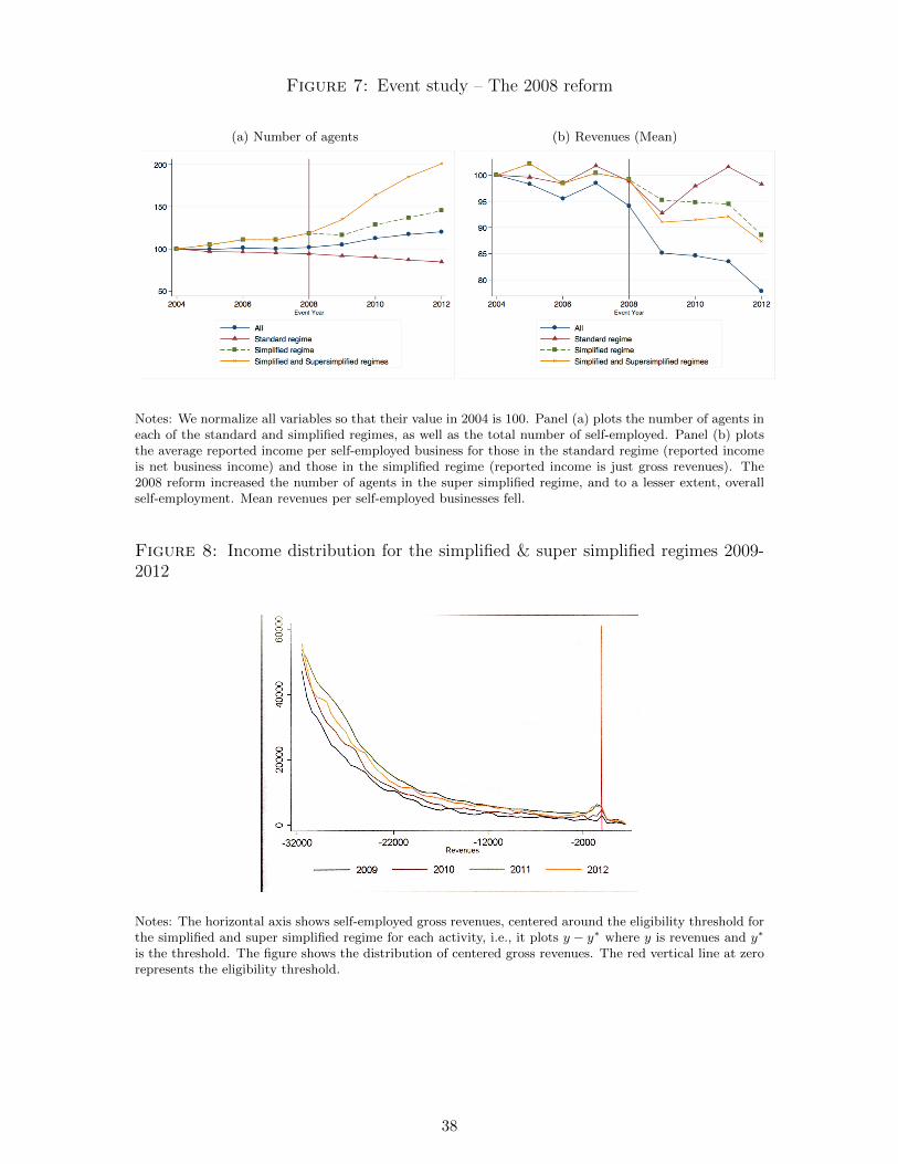
Figure 7: Event study – The 2008 reform

(a) Number of agents (b) Revenues (Mean)

Notes: We normalize all variables so that their value in 2004 is 100. Panel (a) plots the number of agents ineach of the standard and simplified regimes, as well as the total number of self-employed. Panel (b) plotsthe average reported income per self-employed business for those in the standard regime (reported incomeis net business income) and those in the simplified regime (reported income is just gross revenues). The2008 reform increased the number of agents in the super simplified regime, and to a lesser extent, overallself-employment. Mean revenues per self-employed businesses fell.

Figure 8: Income distribution for the simplified & super simplified regimes 2009-2012

Notes: The horizontal axis shows self-employed gross revenues, centered around the eligibility threshold forthe simplified and super simplified regime for each activity, i.e., it plots y − y∗ where y is revenues and y∗

is the threshold. The figure shows the distribution of centered gross revenues. The red vertical line at zerorepresents the eligibility threshold.

38

Figure 9: Proportion of agents in the simplified or super simplified regime amongall self-employed (2011)

Notes: The horizontal axis represents self-employed taxable income, as defined in the text Section 4.2:it is i) net income for agents in the standard regime, ii) gross revenues times the net of rebate rate forthose in the simplified regime, and iii) gross revenues for those in the super simplified regime. The reddashed line represents the threshold (converted into taxable income) for the I&C Services, the green dashedline represents the threshold for the Non Commercial activities, and the blue dash-dot line represents thethreshold for the super simplified regime for both I&C Services and Non Commercial Activities.

Figure 10: Proportion of agents in the super simplified regime conditional on beingin any simplified regime (2011)

Notes: The horizontal axis shows self-employed gross revenues, centered around the eligibility threshold forthe simplified and super simplified regime for each activity, i.e., it plots y − y∗ where y is revenues and y∗

is the threshold. The figure represents, for each level of self employed revenues, the fraction of agents thatchoose the super simplified regime among all those eligible and who are in either the super simplified orthe simplified regime.

39

Figure 11: Proportion of agents in the simplified or super simplified regime amongall self-employed 1994-2012, by tax bracket

Notes: The figure shows the Fraction of agents who choose the simplified or super simplified regime amongall self-employed over the full sample period, and by tax bracket. Tax brackets are as defined in Section 2.

Figure 12: Proportion of agents in the simplified or super simplified regime amongall self-employed, by tax bracket (2011)

Notes: See the notes to Figure 9 for an explanation of the construction of taxable income on the horizontalaxis and the definition of the vertical lines representing eligibility thresholds. The figure shows the propor-tion of agents who are eligible for the super simplified regime among all self-employed agents and who dopick the super simplified regime. The results are shown for different tax brackets as defined in Section 2.

40

Figure 13: Fraction choosing the super simplified regime over the simplified regimeby tax brackets and activities

(a) I&C Services

(b) I&C Retail (c) Non Commercial

Notes: The figure shows the fraction of agents who chose the super simplified regime among all those whoare eligible for the super simplified regime and are in either the simplified or the super simplified regime.The results are shown for different tax brackets as defined in Section 2. Each panel shows a different activitytype.

41

Figure 14: Proportion of agents in the super simplified regime conditional on beingin any simplified regime (2011) – By tax bracket

Note: The horizontal axis shows gross revenues. The vertical line is the eligibility threshold for the supersimplified regime. The results are shown for different tax brackets as defined in Section 2.

Figure 15: Proportion of agents in the super simplified regime conditional on beingin any simplified regime (2011) – By activity type

Note: The horizontal axis shows gross revenues. The vertical line is the eligibility threshold for the supersimplified regime. The results are shown for the I&C Services and the Non Commercial Activities.

42

Figure 16: Proportion of agents in the super simplified regime among all self-employed (2011)

Notes: See the notes to Figure 9 for an explanation of the construction of taxable income on the horizontalaxis and the definition of the vertical lines representing eligibility thresholds. The figure shows the propor-tion of agents in the super simplified regime among all those in any self-employed regime who are eligiblefor the super simplified one. The results are shown for different tax brackets as defined in Section 2.

Figure 17: Bunching at the simplified & super simplified regimes – Eligibilitythresholds by period for 1999-2012

Notes: Frequency of agents by bins of (centered) self-employed revenues, pooled for all years 1999-2012. Thevertical red line represents the threshold. The counterfactual distribution (fitted polynomial) is representedby the red curve in the figures. The bunching zone’s area excess mass is colored in yellow. There issignificant bunching, equal to 70% of the average height of the counterfactual distribution within 1,500euros of the notch.

43

Figure 18: Bunching at the simplified & super simplified regimes – Eligibilitythresholds by periods

(a) 1994-1998

(b) 1999-2008 (c) 2009-2012

Notes: Frequency of agents by bins of (centered) self-employed revenues centered around their thresholdand pooled across 1994-1998 (in 18a), 1999-2008 (in 18b) and 2009-2012 (in 18c). The vertical red linerepresents the threshold. The counterfactual distribution (fitted polynomial) is represented by the red curvein the figures. The bunching zone’s area excess mass is colored in yellow. In all cases, there is significantbunching, equal to, respectively 53%, 75%, and 63% of the average height of the counterfactual distributionwithin 1,500 euros of the notch. It seems quite natural that the earlier period 1994-1999 exhibits less andless sharp bunching because the simplified regime’s threshold was very low and thus the regime was notthat desirable to start with.

44

Figure 19: Bunching at the simplified & super simplified regimes – Eligibilitythresholds by tax brackets for 1999-2012

Notes: See the notes to Figure 17. In addition, agents are here split by tax brackets. Bunching is, inproportional terms higher for the high tax rate agents. All results are reported in Table 3.

Figure 20: Bunching at the simplified & super simplified regimes – Eligibilitythresholds by tax brackets for 1999-2008 and 2009-2012

(a) 1999-2008 (b) 2009-2012

Notes: See the notes to Figure 19.

45

Figure 21: Bunching estimates year by year for 1999-2012

Notes: The figure shows the value of the excess mass with its standard error band (the width of which istwo standard errors, centered around the point value), estimated as explained in the text and representedin Figure 22, 23, and 24. The dotted lines represent years with threshold or rebate changes.

Figure 22: Bunching estimates by year 1999-2002

(a) 1999 (b) 2000

(c) 2001 (d) 2002

Notes: See the notes to Figure 17. The black solid vertical line represents the threshold in year t− 1. Thedashed vertical lines represent the threshold for year t− 2. If the threshold has not changed for more thantwo years, it coincides with the year t (current threshold) which is the red vertical line.

46

Figure 23: Bunching estimates by year 2003-2006

(a) 2003 (b) 2004

(c) 2005 (d) 2006

Notes: See the notes to Figure 17. The black solid vertical line represents the threshold in year t− 1. Thedashed vertical lines represent the threshold for year t− 2. If the threshold has not changed for more thantwo years, it coincides with the year t (current threshold) which is the red vertical line.

47

Figure 24: Bunching estimates by year 2007-2012

(a) 2007 (b) 2008

(c) 2009 (d) 2010

(e) 2011 (f) 2012

Notes: See the notes to Figure 17. The black solid vertical line represents the threshold in year t− 1. Thedashed vertical lines represent the threshold for year t− 2. If the threshold has not changed for more thantwo years, it coincides with the year t (current threshold) which is the red vertical line.

48

Figure 25: Bunching after the introduction of the super simplified regime

Notes: See figure 19.

49

Table 7: Summary statistics for the French population and samples 1994-2012

Panel A

All With wage With self- With any

income only employed self-employed

income only income

Age 40.00 40.00 49.00 48.00

Female 0.47 0.48 0.32 0.33

Married and Civil Union 0.50 0.49 0.63 0.62

Children 0.41 0.41 0.39 0.41

Number of Children 0.71 0.71 0.70 0.72

Retired 0.06 0.06 0.17 0.14

Unemployed 0.11 0.11 0.03 0.05

Panel B

Wage Income 19576 20549 0 6005

SE Income 2004 0 32982 29934

Total NS Income 2056 39 33238 30163

Capital Income 2154 1875 5148 6047

Panel C

Zero Tax rate 0.16 0.16 0.15 0.14

Low Tax rate 0.32 0.33 0.23 0.22

Medium Tax rate 0.38 0.39 0.31 0.32

High Tax rates 0.14 0.13 0.31 0.32

Panel D

Population (in mill.) 532.7 497 26.3 35.6

Notes: “With wage income only” refers to individuals with only wage income. “With self-employed income only” refers to individuals

with self-employed income only. “With any self-employed income” refers to people with any self-employment (who may also have

wage income). “All” refers to any individual who earns either some wage income or some self-employed income (or both). All

variables in panels A and C are expressed in percent of the full group represented in each column. “Age” is expressed in years.

Panel B provides average income in each category in constant 2012 euros. Panel D gives the total population in each column for

the whole period. “Unemployed” refers to the fraction who have perceived any unemployment benefits during the year (they must

have also received some self-employed or wage income to be in this table).

50

Table 8: Summary statistics for the French population and samples 1994-1998Panel A

All With wage With self- With any

income only employed self-employed

income only income

Age 40.00 39.00 48.00 47.00

Married and Civil Union 0.56 0.55 0.68 0.68

Children 0.43 0.43 0.42 0.44

Number of children 0.77 0.77 0.76 0.79

Retired 0.08 0.07 0.16 0.14

Panel B

Wage Income 18377 19329 0.00 5275

SE Income 1927 0 30254 28438

Total NS Income 1963 26 30435 28601

Capital Income 1457 1250 3642 4306

Panel C

Zero Tax rate 0.19 0.20 0.16 0.14

Low Tax rate 0.36 0.37 0.26 0.25

Medium Tax rate 0.31 0.31 0.28 0.28

High Tax rates 0.14 0.12 0.30 0.32

Panel D

Population (in mill.) 130 121.2 6.8 8.8

Notes: See Table 7.

51

Table 9: Summary statistics for the French population and samples 1999-2008Panel A

All With wage With self- With any

income only employed self-employed

income only income

Age 40.00 40.00 49.00 48.00

Female 0.46 0.47 0.31 0.31

Married and Civil Union 0.50 0.49 0.64 0.63

Children 0.40 0.40 0.39 0.40

Number of children 0.70 0.70 0.70 0.72

Retired 0.05 0.04 0.16 0.14

Unemployed 0.09 0.10 0.02 0.03

Panel B

Wage Income 19750 20711 0 5824

SE Income 2066 0 34963 32032

Total NS Income 2123 42 35249 32291

Capital Income 2203 1904 5531 6533

Panel C

Zero Tax rate bracket 0.15 0.15 0.14 0.13

Low Tax rate bracket 0.32 0.32 0.22 0.21

Medium Tax rate bracket 0.38 0.38 0.30 0.31

High Tax rates bracket 0.15 0.14 0.33 0.35

Panel D

Population (in mill.) 283.8 265.5 13.7 18.3

Notes: See Table 7.

52

Table 10: Summary statistics for the French population and samples 2009-2012Panel A

All With wage With self- With any

income only employed self-employed

income only income

Age 41.00 41.00 50.00 48.00

Female 0.48 0.49 0.35 0.36

Married and Civil Union 0.45 0.44 0.57 0.55

Children 0.39 0.39 0.36 0.37

Number of children 0.67 0.67 0.63 0.66

Retired 0.07 0.06 0.21 0.17

Unemployed 0.13 0.14 0.04 0.07

Panel B

Wage Income 20470 21503 0 7145

SE Income 1939 0 31506 26980

NS Income 1999 46 31776 27213

Capital Income 2803 2493 6008 6801

Panel C

Zero Tax rate 0.13 0.13 0.18 0.16

Low Tax rate 0.29 0.30 0.20 0.20

Medium Tax rate 0.46 0.47 0.36 0.38

high Tax rates 0.11 0.10 0.26 0.26

Panel D

Population (in mill.) 118.8 110.3 5.8 8.5

Notes: See Table 7.

53

Table 11: Summary statistics by type of activity 1994-2012Panel A

All Industrial and Non Commercial

Commercial (Retail

and Service)

Age 48.00 49.00 46.00

Female 0.33 0.28 0.41

Married and Civil Union 0.63 0.65 0.59

Children 0.41 0.39 0.44

Number of Children 0.73 0.68 0.80

Retired 0.14 0.16 0.11

Unemployed 0.05 0.05 0.05

Panel B

Wage Income 6049 5265 7538

SE Income 30505 22718 45376

Total NS Income 30733 23029 45454

Capital Income 6133 6040 6552

Panel C

Zero Tax rate 0.13 0.16 0.08

Low Tax rate 0.22 0.26 0.14

Medium Tax rate 0.32 0.34 0.29

High Tax rates 0.33 0.24 0.49

Panel D

Population (in mill.) 34,7 22.5 12.6

Notes: See Table 7.

54

Appendix

A.1 Institutional Details

A.1 French Tax System Primer

The French tax schedule typically looks as follows:

Bracket Lower Bond Upper bond Marginal rate

1 y0 = 0 y1 τ1

2 y1 y2 τ2

3 y2 y3 τ3

4 y3 y4 τ4

5 y4 ∞ τ5

In order to determine the tax amount to be paid by a household, the first thing to compute is the

Family coefficient y which is defined as the ratio between taxable income Y and the number of parts

N of the household :

y =Y

N(A1)

The household that has a family coefficient y ∈ [yM−1; yM ] belongs to the bracket M . Then, the

amount of tax the household has to pay is :

T (y,N) = N × [M−1∑m=1

τm × (ym − ym−1) + τM × (y − yM−1)] (A2)

For instance, for a household with a family coefficient y ∈ [y2; y3], we have :

T (y,N) = N × (τ1 × y1 + τ2 × (y2 − y1) + τ3 × (y − y2)) (A3)

Cap of the Family Coefficient

Let’s assume that the number of parts is Nb + Na where Nb is the base number of parts, and Na

is the additional number of parts. To calculate the cap, one first calculates the tax that would apply

without the additional parts: yb = Y/Nb. We must then consider two possible situations : if the

additional number of parts Na (i) does place the household in a higher tax bracket, or (ii) does not

place the household in a higher tax bracket.

Situation 1

55

If the additional number of parts Na does not place the household in a higher tax bracket, then :

T (yb, Nb) = Nb × [

M−1∑m=1

τm × (ym − ym−1) + τM × (yb − yM−1)] (A4)

The difference in taxes is :

T (yb, Nb)−T (y,N) = (Nb−N)×M−1∑m=1

τm×(ym−ym−1)+τM ×(Nbyb−NbyM−1−Ny+NyM−1) (A5)

By definition, we have Y = Nbyb = Ny, then :

T (yb, Nb)− T (y,N) = (Nb −N)×M−1∑m=1

τm × (ym − ym−1) + τM × yM−1(N −Nb) (A6)

We can re-arrange the expression to obtain :

T (yb, Nb)− T (y,N) = (Nb −N)× [M−1∑m=1

τm × (ym − ym−1)− τM × yM−1)] (A7)

Situation 2

If the additional number of parts Na places the household in a higher tax bracket, then :

T (yb, Nb) = Nb × [

M∑m=1

τm × (ym − ym−1) + τM+1 × (yb − yM )] (A8)

The difference in taxes is :

T (yb, Nb)−T (y,N) = (Nb−N)×M−1∑m=1

τm×(ym−ym−1)+τM×(NbyM−NbyM−1−Ny+NyM−1)+τM+1Nb×(yb−yM )

(A9)

A.2 Computational Appendix

56