dna microarrays comp602 bioinformatics algorithms -m werner 2011

DNA Microarrays

Comp602 Bioinformatics Algorithms-m werner 2011

Cell Snapshot

• What if you could capture what a cell is doing at any given instant?

• You could compare diseased cells to normal ones

• You could follow changes over the cell’s lifetime

04/19/23 m werner WIT Comp602 Bioinformatics Algorithms

Expressed Proteins Provide a Snapshot

• In humans every cell (almost) contains genetic coding for all human functions

• i.e. It can express any human protein• But specialized cells only express proteins

appropriate to their function• Further – they only express proteins as needed• Knowing which proteins are expressed by a cell at

any instant reveals information on what kind of cell it is and what it is currently doing


DNA Microarrays to Measure Protein Expression

• Protein expression can be measured efficiently• Given a sample (cytoplasm, bloodstream, etc.)• Can measure mRNA present• A gene is:

– On if the cell is currently transcribing its mRNA– Off otherwise


Probes for mRNA

• To see if a gene is on use a probe• The probe is the DNA complement of the mRNA we

are checking• i.e. if the mRNA has the sequence AGGTATC the

probe would have TCCATAG• So the mRNA would stick to the probe• You may not need the entire gene for the probe• A short oligonucleotide of 25 – 40 base pairs may

suffice


Probing• To test a sample for the expression of a particular

protein• Paint a glass slide with lots of its probes

(complements of its mRNA)• Add a dye to the sample• Bathe the slide in the sample and rinse off• If the protein is being expressed the slide glows

with the dye color • The intensity of the glow indicates the level of the

protein expression


Parallel Probes

• A DNA Microarray allows for simultaneous probes for multiple proteins

• The slide is divided into small squares• The squares are printed (sometimes with

inkjet technology) with the probes• A single slide can test for 1000 or more

proteins


Ink Jet Printing

• Four cartridges are loaded with the four nucleotides: A, G, C,T

• As the printer head moves across the array, the nucleotides are deposited in pixels where they are needed.

• This way (many copies of) a 20-60 base long oligonucleotide are deposited in each pixel.

By Steve Hookway lecture and Sorin Draghici’s book “Data Analysis Tools for DNA Microarrays”


Inkjet Printed Microarrays

Inkjet head, squirting phosphor-ammodites

From Zohar Yakhini04/19/23 m werner WIT Comp602 Bioinformatics Algorithms

cDNA array,Inkjet deposition

In-Situ synthesized oligonucleotide array. 25-60 mers.

Thermal Ink Jet Arrays, by Agilent Technologies

04/19/23 m werner WIT

Comp602 Bioinformatics Algorithms

Wash the slide with two samples labeled with green and red dye

Results:•Green – Sample 1 expressed•Red – Sample 2 expressed•Yellow – Samples 1 and 2 co-expressed

Flash Demo

04/19/23 11Comp602 Bioinformatics Algorithms

http://www.bio.davidson.edu/courses/genomics/chip/chip.html

Two Channel Detection

• Two-channel microarrays are hybridized with cDNA prepared from two samples to be compared (e.g. diseased tissue versus healthy tissue) and that are labeled with two different fluorophores, red and green.

@mw04/19/23 m werner WIT Comp602 Bioinformatics Algorithms

http://en.wikipedia.org/wiki/DNA_hybridization

http://en.wikipedia.org/wiki/Fluorophore

http://upload.wikimedia.org/wikipedia/en/c/c8/Microarray-schema.jpg

Log Ratios

• For a particular protein (gene) we are interested in the ratio of expression between the malignant sample m and the benign sample b.

• The ratio m/b is not symetric. i.e if malignant is more expressed the ratios go from 1 to ∞, but if benign is more expressed the ratios are squeezed between 0 and 1.

• To equalize, take log2(b/n). Now, ratios >1 have logs ranging up from 0 and negative ones ranging down from 0.


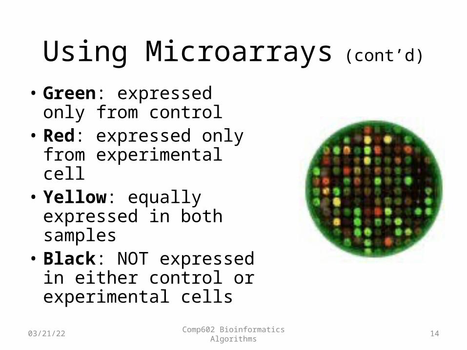
Using Microarrays (cont’d)

• Green: expressed only from control

• Red: expressed only from experimental cell

• Yellow: equally expressed in both samples

• Black: NOT expressed in either control or experimental cells


Microarray Data • Microarray data are usually transformed into an intensity

matrix (below)• The intensity matrix allows biologists to make correlations

between different genes (even if they are dissimilar) and to understand how genes functions might be

related

Time: Time X Time Y Time Z

Gene 1 10 8 10

Gene 2 10 0 9

Gene 3 4 8.6 3

Gene 4 7 8 3

Gene 5 1 2 3

Intensity (expression level) of gene at measured time


Clustering of Microarray Data • Plot each datum as a point in N-dimensional

space• Make a distance matrix for the distance

between every two gene points in the N-dimensional space

• Genes with a small distance share the same expression characteristics and might be functionally related or similar.

• Clustering reveals groups of functionally related genes


Clustering of Microarray Data (cont’d)

Clusters


Homogeneity and Separation Principles

• Homogeneity: Elements within a cluster are close to each other

• Separation: Elements in different clusters are further apart from each other

• …clustering is not an easy task!

Given these points a clustering algorithm might make two distinct clusters as follows


Bad ClusteringThis clustering violates both Homogeneity and Separation principles

Close distances from points in separate clusters

Far distances from points in the same cluster


Good ClusteringThis clustering satisfies both Homogeneity and Separation principles


Clustering Techniques• Agglomerative: Start with every element in

its own cluster, and iteratively join clusters together

• Divisive: Start with one cluster and iteratively divide it into smaller clusters

• Hierarchical: Organize elements into a tree, leaves represent genes and the length of the pathes between leaves represents the distances between genes. Similar genes lie within the same subtrees


Hierarchical Clustering


Hierarchical Clustering: Example


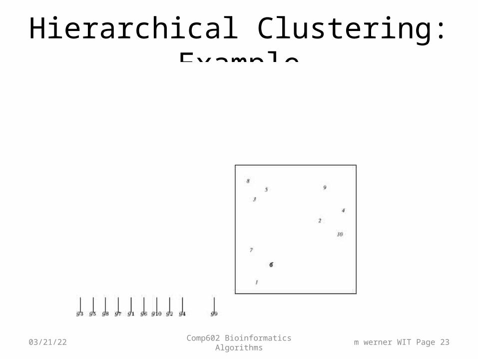
Hierarchical Clustering (cont’d)

• Hierarchical Clustering is often used to reveal evolutionary history


Hierarchical Clustering Algorithm

1. Hierarchical Clustering (d , n)2. Form n clusters each with one element3. Construct a graph T by assigning one vertex to each cluster4. while there is more than one cluster5. Find the two closest clusters C1 and C2

6. Merge C1 and C2 into new cluster C with |C1| +|C2| elements7. Compute distance from C to all other clusters8. Add a new vertex C to T and connect to vertices C1 and C2

9. Remove rows and columns of d corresponding to C1 and C2

10. Add a row and column to d corrsponding to the new cluster C

11. return T

The algorithm takes a nxn distance matrix d of pairwise distances between points as an input.


Hierarchical Clustering Algorithm

1. Hierarchical Clustering (d , n)2. Form n clusters each with one element3. Construct a graph T by assigning one vertex to each cluster4. while there is more than one cluster5. Find the two closest clusters C1 and C2

6. Merge C1 and C2 into new cluster C with |C1| +|C2| elements7. Compute distance from C to all other clusters8. Add a new vertex C to T and connect to vertices C1 and C2

9. Remove rows and columns of d corresponding to C1 and C2

10. Add a row and column to d corrsponding to the new cluster C11. return T

Different ways to define distances between clusters may lead to different clusterings


Hierarchical Clustering: Recomputing Distances

• dmin(C, C*) = min d(x,y) for all elements x in C and y in C*

– Distance between two clusters is the smallest distance between any pair of their elements

• davg(C, C*) = (1 / |C*||C|) ∑ d(x,y) for all elements x in C and y in C*

– Distance between two clusters is the average distance between all pairs of their elements


Squared Error Distortion• Given a data point v and a set of points X, define the distance from v to X

d(v, X)

as the (Euclidian) distance from v to the closest point from X.

• Given a set of n data points V={v1…vn} and a set of k points X, define the Squared Error Distortion

d(V,X) = ∑d(vi, X)2 / n 1 < i < n


Clustering a Heat Map

• Each sample (column) is a point in n-space where n is the number of proteins tested (rows)

• On the top samples are clustered hierarchically into a dendrogram according to some distance measure. Columns have been swapped to show close samples next to each other.

• On the right proteins are clustered to show how closely they are co-expressed in the various samples. Rows have been swapped.


A: Hierarchical cluster analysis of gene expression patterns of normal and cancerous prostate specimens. The dendrogram indicates relationships among samples based on gene expression profiles. Cluster analysis is seen to distinguish malignant from normal prostate (pink branches). Cluster analysis also defines three subtypes of prostate cancer (numbered above) not distinguishable histologically.

A Perspective on DNA Microarrays in Pathology Research and Practice, Jonathan R. Pollack


http://www.ncbi.nlm.nih.gov/pmc/articles/PMC1934527/

http://www.ncbi.nlm.nih.gov/pmc/articles/PMC1934527/

http://www.ncbi.nlm.nih.gov/core/lw/2.0/html/tileshop_pmc/tileshop_pmc_inline.html?title=An%20external%20file%20that%20holds%20a%20picture%2C%20illustration%2C%20etc.%0AObject%20name%20is%20zjh0080773490002.jpg%20%5BObject%20name%20is%20zjh0080773490002.jpg%5D&p=PMC3&id=1934527_zjh0080773490002.jpg

A Data Mining Problem• On a given microarray, we test on the order of 10k

elements in one time• Number of microarrays used in typical experiment is no more than 100.• Insufficient sampling.• Data is obtained faster than it can be processed.• High noise.• Algorithmic approaches to work through this large

data set and make sense of the data are desired.

From “Data Analysis Tools for DNA Microarrays” by Sorin Draghici


A Data Mining Problem

• On a given Microarray we test on the order of 10k elements at a time

• Data is obtained faster than it can be processed

• We need some ways to work through this large data set and make sense of the data



Grouping and Reduction

• Grouping: discovers patterns in the data from a microarray

• Reduction: reduces the complexity of data by removing redundant probes (genes) that will be used in subsequent assays



Unsupervised Grouping: Clustering

• Pattern discovery via grouping similarly expressed genes together

• Three techniques most often used

k-Means ClusteringHierarchical ClusteringKohonen Self Organizing Feature Maps



Clustering Limitations

• Any data can be clustered, therefore we must be careful what conclusions we draw from our results

• Clustering is non-deterministic and can and will produce different results on different runs



K-means Clustering

• Given a set of n data points in d-dimensional space and an integer k

• We want to find the set of k points in d-dimensional space that minimizes the mean squared distance from each data point to its nearest center

• No exact polynomial-time algorithms are known for this problem

“A Local Search Approximation Algorithm for k-Means Clustering” by Kanungo et. al


K-means Algorithm (Lloyd’s Algorithm)

• Has been shown to converge to a locally optimal solution

• But can converge to a solution arbitrarily bad compared to the optimal solution

•“K-means-type algorithms: A generalized convergence theorem and characterization of local optimality” by Selim and Ismail

•“A Local Search Approximation Algorithm for k-Means Clustering” by Kanungo et al.

K=3

Data Points

Optimal Centers

Heuristic Centers


Distance Measures Between Two Datapoints in n-Space

• Euclidean Distance• Cosine Coefficient – Compare 2 vectors for direction using the dot

product:• x∙y = ∑xi∙yi = |x||y|cos(Ѳ )

• Manhattan Distance• Pearson Correlation Coefficient


Pearson Correlation Coefficient, r. values in [-1,1] interval

• Gene expression over d experiments is a vector in Rd, e.g. for gene C: (0, 3, 3.58, 4, 3.58, 3)

• Given two vectors X and Y that contain N elements, we calculate r as follows:

Cho & Won, 2003


Euclidean Distance

n

iiiE yxyxd

1

2)(),(

543),( 22 AOd E

Now to find the distance between two points, say the origin and the point (3,4):

Simple and Fast! Remember this when we consider the complexity!



Finding a Centroid

We use the following equation to find the n dimensional centroid point amid k n dimensional points:

),...,2

,1

(),...,,( 11121 k

xnth

k

ndx

k

stxxxxCP

k

ii

k

ii

k

ii

k

Let’s find the midpoint between 3 2D points, say: (2,4) (5,2) (8,9)

)5,5()3

924,

3

852(

CP



K-means Algorithm1. Choose k initial center points randomly2. Cluster data using Euclidean distance (or other distance

metric)3. Calculate new center points for each cluster using only

points within the cluster4. Re-Cluster all data using the new center points

1. This step could cause data points to be placed in a different cluster

5. Repeat steps 3 & 4 until the center points have moved such that in step 4 no data points are moved from one cluster to another or some other convergence criteria is met

From “Data Analysis Tools for DNA Microarrays” by Sorin Draghici04/19/23 m werner WIT Comp602 Bioinformatics Algorithms

An example with k=2

1. We Pick k=2 centers at random

2. We cluster our data around these center points

Figure Reproduced From “Data Analysis Tools for DNA Microarrays” by Sorin Draghici


K-means example with k=2

3. We recalculate centers based on our current clusters




4. We re-cluster our data around our new center points




5. We repeat the last two steps until no more data points are moved into a different cluster



Choosing k

• Use another clustering method• Run algorithm on data with several different

values of k• Use advance knowledge about the

characteristics of your test– Cancerous vs Non-Cancerous



Cluster Quality

• Since any data can be clustered, how do we know our clusters are meaningful?– The size (diameter) of the cluster vs. The inter-cluster

distance– Distance between the members of a cluster and the

cluster’s center– Diameter of the smallest sphere



Cluster Quality Continued

size=5

size=5distance=20

distance=5

Quality of cluster assessed by ratio of distance to nearest cluster and cluster diameter



Cluster Quality Continued

Quality can be assessed simply by looking at the diameter of a cluster

A cluster can be formed even when there is no similarity between clustered patterns. This occurs because the algorithm forces k clusters to be created.

From “Data Analysis Tools for DNA Microarrays” by Sorin Draghici04/19/23 55Comp602 Bioinformatics Algorithms

Characteristics of k-means Clustering

• The random selection of initial center points creates the following properties– Non-Determinism– May produce clusters without patterns

• One solution is to choose the centers randomly from existing patterns



Squared Error Distortion• Given a data point v and a set of points X, define the distance from v to X

d(v, X)

as the (Euclidian) distance from v to the closest point from X.

• Evaluate the error induced by mapping each data point to one of the k-means centroids

• Given a set of n data points V={v1…vn} and a set of k centroids X={c1…ck}, define the Squared Error Distortion

d(V,X) = ∑d(vi, X)2 / n 1 < i < n

Algorithm Complexity

• Linear in the number of data points, N• Can be shown to have time of cN

– c does not depend on N, but rather the number of clusters, k

• Low computational complexity• High speed



K-Means Clustering: Lloyd Algorithm1. Lloyd Algorithm2. Arbitrarily assign the k cluster centers3. while the cluster centers keep changing4. Assign each data point to the cluster Ci

corresponding to the closest cluster representative (center) (1 ≤ i ≤ k)

5. After the assignment of all data points, compute new cluster representatives according to the center of gravity of each

cluster, that is, the new cluster representative is ∑v / |C| for all v in C for every cluster C

*This may lead to merely a locally optimal clustering.

0

1

2

3

4

5

0 1 2 3 4 5

expression in condition 1

exp

ressio

n in

co

nd

itio

n 2

x1

x2

x3

0

1

2

3

4

5

0 1 2 3 4 5


exp

ress

ion

in c

on

dit

ion

2

x1

x2

x3

0

1

2

3

4

5

0 1 2 3 4 5


exp

ress

ion

in c

on

dit

ion

2x1

x2

x3

0

1

2

3

4

5

0 1 2 3 4 5


exp

ress

ion

in c

on

dit

ion

2x1

x2x3

Conservative K-Means Algorithm• Lloyd algorithm is fast but in each iteration it moves

many data points, not necessarily causing better convergence.

• A more conservative method would be to move one point at a time only if it improves the overall clustering cost

– The smaller the clustering cost of a partition of data points is the better that clustering is

– Different methods (e.g., the squared error distortion) can be used to measure this clustering cost

K-Means “Greedy” Algorithm1. ProgressiveGreedyK-Means(k)2. Select an arbitrary partition P into k clusters3. while forever4. bestChange 05. for every cluster C6. for every element i not in C7. if moving i to cluster C reduces its clustering cost8. if (cost(P) – cost(Pi C) > bestChange9. bestChange cost(P) – cost(Pi C) 10. i* I11. C* C12. if bestChange > 013. Change partition P by moving i* to C*

14. else15. return P

dna microarrays comp602 bioinformatics algorithms -m werner 2011

Documents

slide glows

single slide

glass slide

expressed proteins

green sample

human protein

red sample

cell snapshot