d.matthes- convergence in discrete cauchy problems and applications to circle patterns

8/3/2019 D.Matthes- Convergence in Discrete Cauchy Problems and Applications to Circle Patterns

http://slidepdf.com/reader/full/dmatthes-convergence-in-discrete-cauchy-problems-and-applications-to-circle 1/23

CONFORMAL GEOMETRY AND DYNAMICSAn Electronic Journal of the American Mathematical SocietyVolume 00, Pages 000–000 (Xxxx XX, XXXX)S 1088-4173(XX)0000-0

CONVERGENCE IN DISCRETE CAUCHY PROBLEMS

AND APPLICATIONS TO CIRCLE PATTERNS

D. MATTHES

Abstract. A lattice-discretization of analytic Cauchy problems in two di-mensions is presented. It is proven that the discrete solutions converge to asmooth solution of the original problem as the mesh size ε tends to zero. Theconvergence is in C ∞ and the approximation error for arbitrary derivativesis quadratic in ε. In application, C ∞-approximation of conformal maps bySchramm’s orthogonal circle patterns and lattices of cross-ratio minus one isshown.

1. Introduction

In the flourishing field of discrete differential geometry, classical geometrical objectsare matched by discrete counterparts which inherit many qualitative features of thesmooth originals. Discretizations have been proposed for a large variety of surfaces,coordinate systems and maps, see [BP2] for an overview.Special attention has been devoted to circle packings in the plane and their relationto conformal mappings. The fundamental question of quantitative approximation has been intensively studied. As a key result in this context, Thurston’s conjectureon the convergence of hexagonal circle packings to the Riemann map was proven

by Rodin and Sullivan [RS] in 1987. Their result has been improved in many ways.For instance, hexagonal packings were shown to converge in C ∞ [HS], and the errorfor the approximation and its derivatives was estimated [DHR].An alternative approach to a discrete theory of conformal maps is provided bycircle patterns. Generally, a circle pattern with square-grid combinatorics is acorrespondence that assigns to any vertex of the Z2-lattice a circle in the complexplane. As the collection of image circles inherits the square-grid combinatorics,there is a natural notion of neighbors and elementary quadruples (circles assigned tothe corners of aZ2-square). One requires that the circles of an elementary quadrupleintersect in one point. Thus, each circle has four points of intersection with itsneighbors. The intersection points form a lattice with square-grid combinatorics ontheir own.

Additional conditions are imposed to single out subclasses of more rigid patterns.The most prominent subclass is provided by “orthogonal circle patterns” introducedby Schramm [Sch], also called Schramm-patterns in the following. The additionalconstraint is that neighboring circles intersect orthogonally.

2000 Mathematics Subject Classification. Primary 30G25 ; Secondary 35A10, 52C15.Supported by the SFB 288 “Differential Geometry and Quantum Physics” of the Deutsche

Forschungsgemeinschaft.

c1997 American Mathematical Society

1



2 D. MATTHES

As a second possibility, one requires that the four points of intersection on eachcircle have cross ratio minus one. In this situation, it is preferred to consider the

lattice of intersection points rather than the circles themselves. One obtains cross-ratio-lattices or CR-mappings, which were first investigated by Nijhoff et al [NQC].Generalizing CR-mappings to immersions in three-space, a definition of discreteisothermic surfaces was obtained by Bobenko and Pinkall [BP1].In comparison to (especially hexagonal) packings, much less in known about theapproximation properties of circle patterns. The C 0-convergence theorem in [Sch]seems to be the only result in this direction so far. In this article, it is proven thatan arbitrary planar conformal map u : Ω ⊂ C → C can be locally approximatedby a sequence of Schramm-patterns and CR-mappings. More precisely: intersectthe domain Ω with a square grid of mesh size ε > 0, obtaining a discrete setΩε. A suitable circle pattern from the respective class can be defined on each Ωε,so that the circle centers (Schramm-pattern) or intersection points (CR-mapping)approximate the values of u at corresponding sites with an error O(ε2). Moreover,the convergence is in C ∞. This means that arbitrary partial derivatives of u areuniformly approximated by the respective difference quotients calculated from thecircle pattern, also with an error of order O(ε2).The analytic background for the geometric convergence result is of interest on itsown. A discrete approximation theory for analytic Cauchy problems is developedin this article. Its applications are not limited to geometrical questions. More-over, a new proof of the Cauchy-Kovalevskaya theorem – based on purely discreteconstructions – is obtained as a by-product.Consequently, the presented approach to circle patterns differs in nature fromSchramm’s where a boundary value problem was considered and techniques from(discrete) elliptic theory played an important role. Instead, our proof combinesthese two ingredients: the first are methods which were developed for Cauchy prob-

lems associated with discrete hyperbolic equations. These have already been used toshow C ∞-convergence of discrete orthogonal coordinate systems [BMS]. The otheringredient is an adaptation of fundamental ideas from the proof of the (abstract)Cauchy-Kovalevskaya theorem [Nag],[Nir]. In particular, a discrete counterpart of the scale of spaces of analytic functions is defined.For definiteness, let us consider the Cauchy problem

∂ tu(t, x) = M∂ xu(t, x) + f (u(t, x)),(1.1)

u(0, x) = u0(x).

The continuous solution u : Ω → Cd is sought on Ω ⊂ R

2, where M is a constantd

×d-matrix, and f is an analytic function. For x-analytic data u0, there exists a

local solution to (1.1) by the Cauchy-Kovalevskaya theorem.A variety of elliptic equations – e.g., the nonlinear Poisson equation (∂ 2x + ∂ 2t )u =f (u) – can be brought into the standard form (1.1). In the case of most interesthere, u is a conformal map. Identifying the (t, x)-plane with the complex numbers,u(t, x) : Ω → C is holomorphic in z = x+it, and hence solves the Cauchy-Riemann-equations, which is (1.1) with M = i and f ≡ 0.Circle patterns are constructed which approximate u. These are characterized bydiscrete functions vε on two-dimensional grids Ωε ⊂ Ω of mesh-size ε > 0. Thecrucial observation is that the vε solve a discrete equation similar to (1.1), where



CONVERGENCE IN DISCRETE CAUCHY PROBLEMS 3

derivatives are replaced by difference quotients. The content of the developed ap-proximation theory is that the discrete solutions vε converge to u in C ∞. Eventu-

ally, this leads to convergence of the corresponding circle patterns.The article is organized as follows: in section 2, the theorem about discrete approxi-mation of the Cauchy problem (1.1) is formulated. The theorem is proven in section3. Its numerical applicability is discussed in section 4. Convergence theorems forCR-mappings and Schramm-patterns are proven in sections 5 and 6, respectively.

Acknowledgments. The author would like to thank Alexander Bobenko and YuriSuris for many discussions and helpful advice. Further, the author is grateful toWalter Craig for an entertaining introduction to the topic of abstract Cauchy-Kovalevskaya theorems.

2. Discrete Approximation of the Cauchy Problem

As usual, a function f : D

⊂C p

→Cd is called analytic, if it is complex differ-

entiable in its p arguments. Moreover, a function u : Iξ → Cd defined on the realinterval Iξ = [−ξ, +ξ] is called analytic if it extends to a complex differentiablefunction on Bρ(Iξ) = x ∈ C | dist(x, Iξ) ≤ ρ for an appropriate choice of ρ > 0.By abuse of notation, there will be no distinction between u and and its uniquelydetermined complex extension.Consider problem (1.1) under the following assumptions: The d × d-matrix M isconstant, f is an analytic function near u0(0), and the initial datum u0 is analyticon an interval Iξ. Solutions u = (u(1), . . . , u(d)) : Ω → C

d are sought on diamond-shaped domains

Ω = Ω(r) = (t, x) ∈ R2 : |x| + |t| ≤ r.

The Cauchy-Kovalevskaya-Theorem implies

Theorem 2.1. Problem (1.1) has a classical solution u on Ω = Ω(r) for a suitabler < ξ. This solution is x-analytic and t-smooth, i.e., of class C ∞.

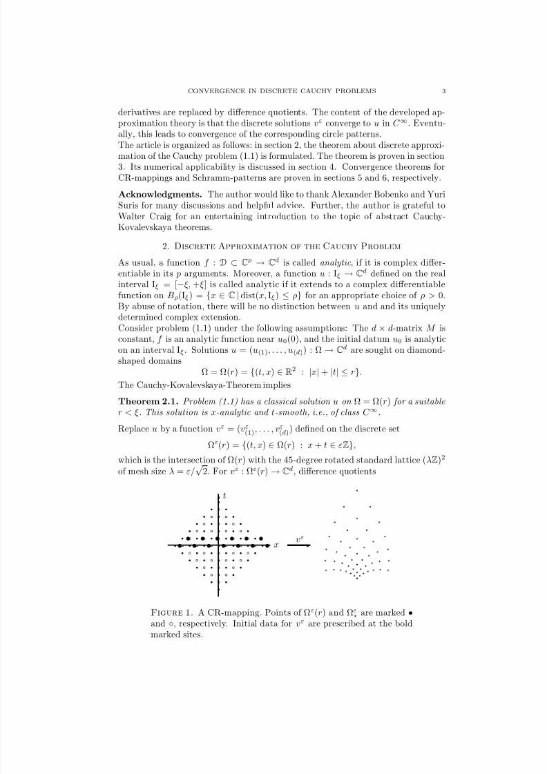
Replace u by a function vε = (vε(1), . . . , vε(d)) defined on the discrete set

Ωε(r) = (t, x) ∈ Ω(r) : x + t ∈ εZ,

which is the intersection of Ω(r) with the 45-degree rotated standard lattice (λZ)2

of mesh size λ = ε/√

2. For vε : Ωε(r) → Cd, difference quotients

q

q

q

q

q

q

q

q

q

q

q

q

q

q

q

q

q

q

q

q

q

q

q

q

q

q

q

q

q

q

q

q

q

q

q

q

q

q

q

q

q

q

q

q

q

q

q

q

q a

a

a

a

a

a

a

a

a

a

a

a

a

a

a

a

a

a

a

a

a

a

a

a

a

a

a

a

a

a

a

a

a

a

a

a s s s s s s s

s s s s s s

- x

6t

-vε

Figure 1. A CR-mapping. Points of Ωε(r) and Ωε∗ are marked •

and , respectively. Initial data for vε are prescribed at the boldmarked sites.



4 D. MATTHES

(δxvε)(t, x) = 1ε

vε(t, x + ε

2) − vε(t, x − ε

2)

(δtvε)(t, x) = 1

ε vε(t + ε2

, x)

−vε(t

−ε2

, x) ,

are given on the dual lattice

Ωε∗(r) = (t, x) ∈ Ω(r − ε

2) : ε

2+ x + t ∈ εZ.

Higher difference quotients δmx δnt vε are defined on

Ωεm+n(r) =

Ωε(r − (m + n) ε2 ) if m + n is even,Ωε∗(r − (m + n) ε

2) if m + n is odd.

Replace the Cauchy problem (1.1) by the discrete problem

(2.1)δtvε(t, x) = M δxvε(t, x) + f ε(vε)(t, x) ((t, x) ∈ Ωε

∗)vε(0, x) = vε0(x) ((0, x) ∈ Ωε)vε( ε2 , x) = vε+(x) (( ε2 , x) ∈ Ωε

∗)

For t 0, the nonlinearity f ε(vε)(t, x) is of the form

f ε(vε)(t, x) = F ε(vε(t, x ± ε2 ), vε(t, x ε

2 ), vε(t ε2 , x)).

Theorem 2.2. Assume that u0 is analytic on I ξ, that f is analytic on a neighbor-hood D ⊂ C

d of u0(0) and F ε is analytic on D × D × D ⊂ C3d for each ε > 0.Furthermore, assume that

(2.2) |F ε(u+, u−, u∗) − f (u++u−

2 )| ≤ K (ε + |u+−u−|)2

holds for all u+, u−, u∗ ∈ D with K > 0 independent of ε.Then there is some r < ξ such that the solutions vε to problem (2.1) with

(2.3)vε0(x) = u0(x) ((0, x) ∈ Ωε(r))

vε+(x) = u0(x) + ε2

M ∂ xu0(x) + f (u0(x))

(( ε

2, x) ∈ Ωε

∗(r))

are C ∞-convergent to a smooth function u on Ω(r) with an error O(ε2). Moreprecisely, for arbitrary m, n ≥ 0, there are constants C mn > 0 so that

sup(t,x)∈Ωεm+n(r) |∂ mx ∂ nt u(t, x) − δmx δnt vε(t, x)| ≤ C mnε2.(2.4)

The function u constitutes a classical solution to the Cauchy problem (1.1).

In particular, Theorem 2.2 implies the classical existence Theorem 2.1.

Example 2.3 (A Nonlinear Elliptic Problem). Rewrite the elliptic initial valueproblem

∂ 2t φ(t, x) + ∂ 2xφ(t, x) = g(φ(x, t))(2.5)

φ(0, x) = φ0(x), ∂ tφ(0, x) = φ+(x)(2.6)

for the scalar function φ in the form of problem (1.1):

(2.7) ∂ t

u(1)

u(2)

u(3)

=

0 0 0

0 0 10 −1 0

∂ x

u(1)

u(2)

u(3)

+

u(3)

0g(u(1))

,

denoting u(1) = φ, u(2) = ∂ xφ and u(3) = ∂ tφ. For functions φ0, φ+ analytic onIξ, the respective initial data u0(1)(x) = φ0(x), u0(2) = ∂ xφ0(x), u0(3) = φ+(x) areanalytic, too. Assuming further that the nonlinearity g is analytic near φ0(0), asolution to (2.7) exists on some Ω = Ω(r). The constraint ∂ xu(1) = u(2) propagates,so φ := u(1) indeed solves (2.5).




In order to approximate (2.7) by a discrete problem (2.1), choose

F ε(v+, v−, v∗) = 1

2

(v+(3) + v−(3), 0, g(v+

(1)) + g(v−(1)))

as nonlinearity, independent of ε. The assumptions of Theorem 2.2 concerninganalyticity and boundedness of F ε are obviously fulfilled. A Taylor expansion of garound V = (v+

(1) + v−(1))/2 proves the estimate (2.2):

12 (g(v+

(1)) + g(v−(1))) = g(V ) + 12 (v+

(1)− v−(1))g(V ) + O(|v+ − v−|2),

Hence, the component vε(1) of the discrete solutions to problem (2.1) converges to

the smooth solution φ on Ω(r) with a suitable positive r < ξ in the sense of (2.4).

3. Proof of Theorem 2.2

The proof consists of three parts: in the first, a smooth solution u to (1.1) isconstructed as the limit of a suitable sequence of discrete solutions vε to (2.1).

Secondly, C 0-approximation of u is shown, i.e., (2.4) for m = n = 0. Finally, aninduction argument yields (2.4) for arbitrary m, n.The proof combines elements from discrete approximation theory for hyperbolicPDE [BMS] with ideas from Walter’s proof [Wal] of the Cauchy-Kovalevskaya the-orem, which is based on the classical papers [Nir], [Nag]. Recall the strategy of the latter. A solution u to (1.1) is constructed such that u(t, x) is x-analytic onthe time-dependent domain Bρ(t)(Iξ(t)) for any t ∈ [−T, +T ]. The size parametersρ(t), ξ(t) decreases as |t| increases. The motivation is that ∂ x is a bounded operatorbetween the spaces of analytic functions on Bρ(Iξ) and on Bρ(Iξ), respectively,for any ρ < ρ and ξ ≤ ξ. The norm of ∂ x is determined by the classical Cauchyestimate

supx∈Bρ(Iξ)

|∂ xu(x)

| ≤(ρ

−ρ)−1supx∈Bρ (Iξ)

|u(x)

|.(3.1)

Introducing suitable time-dependent norms · t for u(t), an a priori estimate of Gronwall type is derived from (3.1),

u(t)t ≤ u00 +

t0

C (t, s)u(s)s ds.(3.2)

Eventually, (3.2) enables one to obtain the solution u as the fixed point of a con-tracting map.Time-dependent norms for discrete functions are introduced in the following. Toprove approximation of u by vε, a discrete analogue of (3.2) is derived for the t-norm of the difference wε(t) := u(t) − vε(t). More precisely, wε(t) at time t = n ε

2is estimated in terms of wε(t − ε

2) and wε(t − ε), leading to the discrete Gronwall

estimate in (3.16). The crucial technical tool is a discrete version of the Cauchy

estimate (3.1), which is given in Lemma 3.1 below.

3.1. Notations. Let D(ρ) ⊂ C denote the complex disc of radius ρ centered at 0,and for p > 1, D p(ρ) = D(ρ) × · · · × D(ρ) ⊂ C

p is a p-dimensional poly-disc. Also,recall that Iξ = [−ξ, +ξ] and Bρ(Iξ) = z ∈ C | dist(z, Iξ) ≤ ρ.The crucial quantity that determines most of the following constructions is r > 0,the appropriate diameter of the domain Ω(r), which has to be found. From r, onedefines

ξ(t) = r − |t|, ξn = r − |n| ε2 , ρ(t) = 3r − 2|t|, ρn = 3r − |n|ε.



6 D. MATTHES

Discrete intervals containing m + 1 points are given by

I

ε

m = −m2

ε , . . . ,

−ε, 0, ε , . . . , m

2ε

if m is even

−m2 ε , . . . , − ε

2 , ε2 , . . . , m2 ε if m is odd

For a function v : Iεm → Cd, define its difference quotient, ε

2-shift, restriction and

linear interpolation:

δxv : Iεm−1 → Cd, (δxv)(x) = 1

ε

v(x + ε

2) − v(x − ε

2)

τ xv : Iεm−1 → Cd, (τ xv)(x) = v(x + ε

2 ), (τ −1x v)(x) = v(x − ε

2 )

πv : Iεm−2 → Cd, (πv)(x) = v(x)

Ev : I ε2m

→ Cd, (Ev)(x) =

x − xε−

εv(xε

+) +xε

+ − x

εv(xε

−).

Here xε−, xε

+ ∈ Iεm are such that xε− ≤ x < xε

+ and xε+ = xε

− + ε. The restriction

of a function u : Ω(r)

→Cd to the discrete domain Ωε(r) is denoted by [u]ε. For

the discrete function v : Ωε(r) → Cd, let vn be its restriction to time t = n ε2 , sovn(x) = v(n ε

2, x), which is defined on the interval Iεn where n is the largest integer

with ε2 n ≤ ξn.

In these notations, the problem (2.1) takes the convenient form (n > 0):

vεn+1 = πvεn−1 + εδxvεn + εf εn(vε)(3.3)

f εn(vε) = F ε(τ xvεn, τ −1x vεn, πvε

n−1)(3.4)

where pointwise evaluation of the arguments is understood.Without loss of generality, assume that |M u| ≤ |u| for all u ∈ C

d, and thatu0(0) = 0. Indeed, this can be achieved by a dilation of the t-axis and an affinetransformation of the values of u, respectively. For an appropriate choice of U > 0,f is defined on Dd(3U ) and F ε on D3d(3U ), respectively.

3.2. Discrete norms and their properties. For ρ > 0, define a functional onscalar discrete functions v : Iεm → C by

vρ =

nk=0

ρk

k!max

x∈Iεm−k

|δkv(x)|.

For multi-component functions v = (v(1), . . . , v( p)) : Iεm → C p, let

vρ = maxi=1,...,p

v(i)ρ.

These norms share several properties with the maximum-norm of analytic functionsover a complex domain.

Lemma 3.1. The functionals

· ρ provide a scale of norms on discrete functions.

For u : Iεn → Cd and 0 ≤ ρ ≤ ρ, one has uρ ≤ uρ. In addition, each · ρ hasthe following properties:

(1) Absolute bound: |u(x)| ≤ uρ for all x ∈ Iεn.(2) Submultiplicativity: u vρ ≤ uρvρ for scalar functions u and v.(3) Discrete Cauchy estimate: For θ > 0, uρ + θδxuρ ≤ uρ+θ.(4) Restriction estimate: If u : Iξ → C

d extends analytically to Bρ(Iξ) and uε

is its restriction to Iεn ⊂ Iξ, then, provided ρ < ρ,

(3.5) uερ ≤ (1 − ρ/ρ)−1supBρ (Iξ)|u|




(5) Analyticity estimate: Let be given functions vε : Iεnε → Cd with nεε ≥

ξ ≥ 0 and vερ ≤ C for a sequence ε → 0. Then there exists an analytic

u : Iξ → Cd, so that Eδkxvε(k) converges to ∂ kxu uniformly for each k ≥ 0and a suitable subsequence ε(k) → 0 of ε. Moreover, u possesses a complex extension to Bρ(Iξ) which is bounded by C .

This lemma is proven in the appendix.A norm with properties (1) and (2) will be called submultiplicative norm in thefollowing. For an arbitrary submultiplicative norm, the following lemma holds:

Lemma 3.2. Let the analytic function f : D p(U ) → C satisfy

|f (u)| ≤ C(|u(1)|, . . . , |u( p)|) for all u ∈ D p(U ), with some function C ≥ 0 that is non-decreasing in each of itsarguments. Then for each γ > 1 and every discrete function v : Iεn → C

p with

γ vρ ≤ U , the composition f (v) is well-defined on Iε

n, and (3.6) f (v)ρ ≤ ΓC(γ v(1)ρ, . . . , γ v( p)ρ).

The constant Γ depends on γ but not on the submultiplicative norm · ρ.

This lemma is proven in the appendix. Two cases of particular interest are

f (v)ρ ≤ Γ supDp(U )

|f |(3.7)

f (v1) − f (v2)ρ ≤ Γ supDp(U )

|f | v1 − v2ρ(3.8)

which hold for all v, v1, v2 with vρ ≤ U/γ and v1ρ, v2ρ ≤ U/(2γ ), respec-tively, with γ > 1 arbitrary and Γ = Γ(γ ).Estimate (3.7) follows immediately with C

≡supDp(U )

|f

|in (3.6). To obtain (3.8),

consider the function f (a, b) := f (a + b, a − b) which is analytic in a, b ∈ D p(U/2),and let C(|a|, |b|) := supDp(U ) |f | |b|. Now let a = (v1 + v2)/2 and b = (v1 − v2)/2.

3.3. Existence of a Continuous Solution. In the following, it will be shownthat for an appropriate r > 0 and ε small enough, discrete solutions vε exist onΩε(r), and a limiting function u can be defined on Ω(r). In fact, r > 0 will bedefined so that the solutions vε on Ωε(r) satisfy

vεnσn ≤ U, σn = ρn + r = 4r − nε(3.9)

for all n with ε2|n| ≤ r – recall that vεn(x) = vε(n ε

2, x). Choose U > 0 suitable

and let F > 0 be an ε-independent bound for F ε on D3d(3U ). The basic idea is toderive (3.9) inductively as follows:

Mεn := vεn+1σn + vεnσn ≤ U ( 12 + n2N )(3.10)

To obtain (3.10) at n = 0, observe that the functions

u0 and u0 + ε2 (M ∂ xu0 + f (u0))

are analytic on a complex neighborhood of x = 0. It follows that if r and ε aresmall enough, then the initial data (2.3) satisfies

vε04r, vε+4r ≤ U 4

,

taking into account that u0(0) = 0 and using property (4) of Lemma 3.1.



8 D. MATTHES

Now suppose (3.10) holds at n ≥ 0. Then f εn(vε) is defined on Iεn, and

Mn+1

≤ vεn

σn+1 + ε

δxvεn

σn+1

≤vεn−1σn+1+ε

+ε

f εn(vε)σn+1

≤ΓF

+

vεnσn+1

≤ Mn + εΓF .

To estimate δxvε and f ε(vε), property (3) of Lemma 3.1 and inequality (3.7) wereemployed, respectively.In addition to |vε| ≤ U , estimates on the difference quotients follow:

|δxvε| ≤ maxn

(σ−1n vεnσn) ≤ U/(2r)(3.11)

|δtvε| ≤ |δxvε| + |f ε(vε)| ≤ U/r + ΓF (3.12)

|δ2xvε| ≤ max

n(2σ−2

n vεnσn) ≤ U/(2r2).(3.13)

For each ε, let vεI be the restriction of vε to points (x, t)∈

Ωε(r) with “even” timecoordinate, t = (2k) ε2 . Note that vεI is defined on a sublattice of (εZ)2. Define thefamily vεI ε of continuous functions obtained from x-t-linear interpolation of vεI onΩ(r). By the estimates (3.11) and (3.12), this family is equicontinuous. Hence, the

Arzel‘a-Ascoli theorem applies: there is a sequence ε → 0 such that vε

I convergesto a smooth limit uI uniformly on Ω(r). Moreover, by (3.13), it is possible to

choose the sequence ε such that also δxvε

I converges uniformly to ∂ xuI (cf. theproof of property (5) in Lemma 3.1). The same procedure is applicable to vεII , therestriction to the “odd” time values t = (2k + 1) ε

2; choose a subsequence ε of ε

such that vε

II → uII and δxvε

II → ∂ xuII . Also, f εn(vε

I ) with even n converges tof (uI ) uniformly as can be deduced from the estimate (2.2) – and respectively for

n odd, f εn(vε

II ) → f (uII ).Since vε solves (3.3), it follows for all (t, x), (t, x)

∈Ω(r),

vε

I (t, x) = vε

I (t, x) + tt

(δxvε

II (s, x) + f ε

(vε

II )(s, x)) ds + O(ε).

Passing to the uniform limit as ε → 0:

uI (t, x) = uI (t, x) + tt (∂ xuII (s, x) + f (uII )(s, x)) ds.

The roles of uI and uII can be interchanged. Consequently, both functions aredifferentiable in time and satisfy

∂ t

uI

uII

=

0 M

M 0

∂ x

uI

uII

+

f (uII )f (uI )

.(3.14)

By property (5) of Lemma 3.1, the estimates vεnσn ≤ U imply for fixed t ∈ [−r, r]that uI/II (t, x) extend x-analytically to Br+ρ(t)(Iξ(t)), where they are bounded byU . And since uI/II solve the equation (3.14), their analytic continuations do as well.So uI and uII are smooth with respect to t, as any t-derivative can be expressed interms of x-derivatives and compositions with the analytic function f .The pair (uI , uII ) is the only solution to (3.14) of that smoothness. This is seenas follows: In the proof of estimate (2.4) below, u could be any x-analytic andt-smooth solution to the problem (1.1); no reference to the above construction ismade. In particular, estimate (2.4) applies to (uI , uII ) in place of u and the system(3.14) in place of equation (1.1), respectively. But only one smooth function cansatisfy (2.4) for all ε > 0.




For symmetry reasons, the unique solution (uI , uII ) to (3.14) with initial conditionsuI (0, x) = uII (0, x) = u0(x) satisfies uI = uII =: u on Ω(r). Hence, u solves (1.1)

with u(0, x) = u0(x) for x ∈ Ir.

3.4. Approximation in C 0. For shortness, let uε = [u]ε be the restriction of thesmooth solution, and let wε = vε − uε denote the deviation of vε from u. The ideaof the proof is to calculate ε-independent bounds on the expression

Ln := wεn+1ρn + wε

nρn(3.15)

which is defined for ε2|n| ≤ r. Again, only n ≥ 0 is considered here, and the

treatment of n ≤ 0 is left to the reader. It will be shown that

(3.16) Ln ≤ (1 + εB∗)Ln−1 + C ∗ε3 and L0 ≤ D∗ε2,

leading by the standard Gronwall estimate to

(3.17)Ln ≤ (C

∗

+ D

∗

)e

rB∗

ε

2

which implies (2.4) for m ≥ 0 and n = 0.To prove the estimate (3.16) at an instant of time t = εn with n ≥ 1, express wε

n+1

in terms of uε and vε at previous time steps:

Ln+1 ≤ πwεn−1 + δxwε

nρn + wεnρn (A)

+εf εn(vε) − f εn(uε)ρn (B)

+ε(M δxuεn + f εn(uε)) − (δtuε)nρn (C)

The three resulting expressions (A)-(C) as well as the initial conditions

L0 =

wε

0

ρ0 +

wε

1

ρ0 (IC)

are estimated separately in the following.(A) By property (3), and observing that ρn + ε = ρn−1,

(A) ≤ wεnρn + εδxwε

nρn + wεn−1ρn

≤ wεnρn+ε + wε

n−1ρn≤ Ln−1.

(B) With the help of estimate (3.5), one concludes

f ε(vε) − f ε(uε)ρn≤ F ε(τ xvεn, τ −1

x vεn, vεn−1) − F ε(τ xuεn, τ −1

x uεn, uε

n−1)ρn≤ Γsup |DF ε| max(vεn − uε

nρn , vεn−1 − uεn−1ρn)

≤ B∗

Ln−1.The constant B∗ formally depends on ε via supD3d(U ) |DF ε|. But the analytic

function F ε is uniformly bounded on D p(U ) independently of ε because of (2.2),and so are its derivatives. Hence (B) ≤ εB∗Ln−1.(C) Define the functions

Aεx(t, x) = ∂ xu(t, x) − 1

ε (u(t, x + ε2

) − u(t, x − ε2

))(3.18)

Aεt (t, x) = ∂ tu(t, x) − 1

ε (u(t + ε2

, x) − u(t − ε2

, x))(3.19)

Aεf (t, x) = f (u(x, t)) − F ε(u(t, x + ε

2 ), u(t, x − ε2 ), u(x − ε

2 , t)).(3.20)



10 D. MATTHES

For t ∈ [−r, +r], all three functions possess an analytic extension for x ∈ Bρ(t)+r(Iξ(t)).As u is smooth, one trivially has

|Aεx(x, t)| ≤ C xε2 and |Aεt (x, t)| ≤ C tε2.(3.21)

Furthermore, because of estimate (2.2)

|Aεf (x, t)| ≤ K (ε + |u(t, x + ε

2) − u(t, x − ε

2)|)2

+sup |Df |(u(t, x + ε

2) + u(t, x − ε

2))/2 − u(t, x)

≤ C f ε

2.

Subtracting 0 = M ∂ xu + f (u) − ∂ tu from the expression for (C),

(C) = M δx[u]εn + f εn([u]ε) − δt[u]εn − [M ∂ xu + f (u) − ∂ tu]εnρn≤ δx[u]εn − [∂ xu]εnρn + δt[u]εn − [∂ tu]εnρn + f εn([u]ε) − [f (u)]εnρn

≤ [Aε

x]εn

ρn +

[Aε

t ]εn

ρn +

[Aε

f ]εn

ρn

≤ Γ(C x + C t + C f )ε2 = C ∗ε2.

For the conclusive estimate, property (4) of Lemma 3.1 has been used.(IC) Obviously, wε

0 = 0 by (2.3). And vε1 = vε+ is the restriction of uε+ := u0+ ε

2∂ tu0,

which is an x-analytic function on B4r−ε(Ir−

ε2

) and satisfies

|uε+(x) − u( ε

2, x)| ≤ ε2

8sup

0<s<ε/2

|∂ 2t u(s, x)|.

Exploiting the estimate (3.5) yields

L0 ≤ wε1r−ε ≤ D∗ε2.

3.5. Proof of Smooth Approximation. Since u is smooth on Ω(r), derivativesand difference quotients may be interchanged at the cost of O(ε2):

supΩεm+n(r)|∂ mx ∂ nt u − δmx δnt [u]ε| ≤ C (1)

mnε2.

This is a consequence of the more general formula (5.19) given in Lemma 5.5 insection 5. Hence, to prove (2.4) for given m, n, it suffices to show that

|δmx δnt wε(x, t)| ≤ C (2)mnε2.(3.22)

Submultiplicative norms for functions v : Ωε(r) → Rd are given by

v(N )θ =

n≤N

m=1,2,...

θm+n

m!n!sup

(x,t)∈Ωεm+n(r)

|δmx δnt v(x, t)|.

Define positive numbers θN = θ0/(N + 1), where θ0 < r is suitably chosen later. Itis inductively shown that

wε(N )θN ≤ C (3)N ε2(3.23)

with appropriate constants C (3)N . Obviously, (3.23) implies (3.22) with the choice

C (2)mn = C (3)

n m!n!θ−(m+n)n .

Firstly, some properties of the norms are summarized. In contrast to the previouslyconsidered norms · ρ, which are defined for restrictions of v to intervals Iεn, the

· (N )θ above involve the whole time-dependent function v at once. Apart from

that, each · (N )θ constitutes a submultiplicative norm, so Lemma 3.2 applies, and

(3.7), (3.8) hold. Also, the discrete Cauchy estimate (property (3) of Lemma 3.1)




carries over. Furthermore, the restriction estimate (property (4)) reads as follows:If u is a smooth function such that u(t) is x-analytic on Bρ(I) for all t ∈ [−r, +r],

and 0 < θ < ρ, then

[u]ε(N )θ ≤ Γmax

n≤N sup|t|≤r

supx∈Dρ(I)

|∂ nt u(t, x)|,(3.24)

where Γ depends on the ratio θ/ρ only.For N = 0, inequality (3.23) follows from the previous discussion,

wε(0)θ0

≤ maxn

wεnρn = O(ε2)

because θ0 < r ≤ ρn. Now assume (3.23) for N ≥ 0. By definition of · (N )θ , and

since vε solves the discrete equation (2.1),

wε(N +1)θN+1

≤ wε(N )θN+1

+θN+1

N +1δtw

ε(N )θN+1

≤ wε(N )θN+1 + θN+1N +1 δxwε(N )θN+1 + θ0N 2 f ε(uε) − f ε(vε)(N )θN + θ0N 2 ∆ε(N )θN

The Cauchy estimate is applied to the the sum of the first two terms, and inequality(3.8) to the third term. The norm of

∆ε = M δx[u]ε + f ε([u]ε) − δt[u]ε = [Aεx]ε + [Aε

t ]ε + [Aεf ]

ε

with Aεx, Aε

t and Aεf defined as in (3.18)–(3.20), is estimated using (3.24),

∆ε(N )θN

≤ Γmaxn≤N

supx,t

(|∂ nt Aεx| + |∂ nt Aε

t | + |∂ nt Aεf |) ≤ C (4)

N ε2.

In conclusion,

wε(N +1)θN+1

≤ wε(N )θN

+ θ0ΓN 2 sup |Df | wε(N )

θN+ θ0

N 2 C (4)N ε2

≤ (1 + θ0ΓN 2 sup |Df |)C (3)

N + C (4)N ε2.(3.25)

As inequality (3.8) has been applied to estimate f ε(uε) − f ε(vε), it needs to be

checked that uε(N )θN

, vε(N )θN

≤ U . To verify the bound for vε, formally estimatealong the same lines as above

vε(N +1)θN+1

≤ vε(N )θN+1

+ θN+1

N +1δxvε(N )

θN+1+ θ0

N 2 f ε(vε)(N )θN+1

≤ vε(N )θN

+ θ0N 2 ΓF ≤ vε(0)

θ0+ θ0ΓF

n≤N 1/n2.

For simplicity, assume that vε(0)θ0

< 12

U , possibly after diminishing r. As the sum

∞n=0 1/n2 is finite, it can be achieved that vε(N )

θN< 3

4U for all N ≥ 0 by choosing

θ0 small enough. For ε < εN so small that QN ε2 < U/4,

uε(N )θN

≤ vε(N )θN

+ wε(N )θN

≤ U.

This justifies estimate (3.25) and finishes the proof.

4. A Remark on Numerical Applicability

The iteration (3.3) solving the discrete problem (2.1) is tailored to numerical im-plementation. Assume, the values of vεn−1 and vεn are known. Then:

vεn+1(x) = vεn−1(x) + M (vεn(x + ε2 ) − vεn(x − ε

2 )) + εf εn(vε)(x).(4.1)



12 D. MATTHES

To investigate the effect of round-off errors, consider the perturbed quantity vε

solving the modified equation

vεn(x) = vεn+2(x) + M (vεn+1(x + ε2 ) − vεn+1(x − ε

2 )) + εf εn(v)(x) + µn(x).

Usually, only an absolute bound on the round-off error µ is known, |µn(x)| ≤ 10−q.One should think of q as the number of “precise” digits, which is fixed a priori. Toestimate the deviation of vε from u, modify inequality (3.16) in the obvious way:

Ln ≤ (1 + εB∗)Ln+1 + C ∗ε3 + E ∗,

where E ∗ bounds the error introduced by µ. In the worst case, some component of µ takes values +10−q and −10−q interchangingly, so that

E ∗ = µnρn ≈ 10−q exp(r/ε).(4.2)

As before, r is the diameter of the domain Ω. The relation (4.2) predicts instabilityof the discrete equation (4.1). A finer mesh size ε does not necessarily correspond

to a better approximation. One expects that there is an ε0 > 0 – depending on theinitial data u0 and radius r > 0 – such that the approximation error

• decays like ∼ ε2 for ε ε0,• grows dramatically like ∼ e1/ε for ε → 0 and ε < ε0.

From (4.2) it is suggested that ε0 ∼ r/q. The pictures in the following sectionswere calculated with r ≈ 1, ε ≈ 0.1 and q ≈ 10.

5. Cross-Ratio-Equation

The cross-ratio of four mutually distinct complex numbers q1, . . . , q4 ∈ C is

CR(q1, q2, q3, q4) =(q1 − q2)(q3 − q4)

(q2

−q3)(q4

−q1)

.

Consider Ω(R) as a subset of C, i.e, identify each point (t, x) ∈ Ω(R) with thecomplex number z = x + it ∈ C.

Definition 5.1 ([NQC]). A CR-mapping is a lattice-function ψε : Ωε(R) → C suchthat for all z∗ ∈ Ωε

∗(R) ⊂ C

(5.1) CR

ψε(z∗ + ε2

), ψε(z∗ + i ε2

), ψε(z∗ − ε2

), ψε(z∗ − i ε2

)

= −1.

CR-mappings are suitable discrete analogues of holomorphic functions in the sensethat any holomorphic function can be locally approximated.

Theorem 5.2. Assume φ : Ω(R) → C is a holomorphic function with φ(0) = 0.Then there are positive constants r < R and C mn, so that for each ε > 0, a CR-mapping ψε is defined on Ωε(r) and approximates φ in C ∞:

supz∈Ωε

m+n(r)|δmx δnt ψε(z) − ∂ mx ∂ nt φ(z)| ≤ C mnε2.(5.2)

Proof: As a first step, an equation of type (2.1) is derived for an arbitrary CR-mapping ψε : Ωε(R) → C. Denote by T ± the shift operators

(T +h)(z) = h(z + ε2

(i + 1)), (T −h)(z) = h(z + ε2

(i − 1)).

The edges

αε = (T +ψε − ψε)/ε, β ε = (T −ψε − ψε)/ε(5.3)




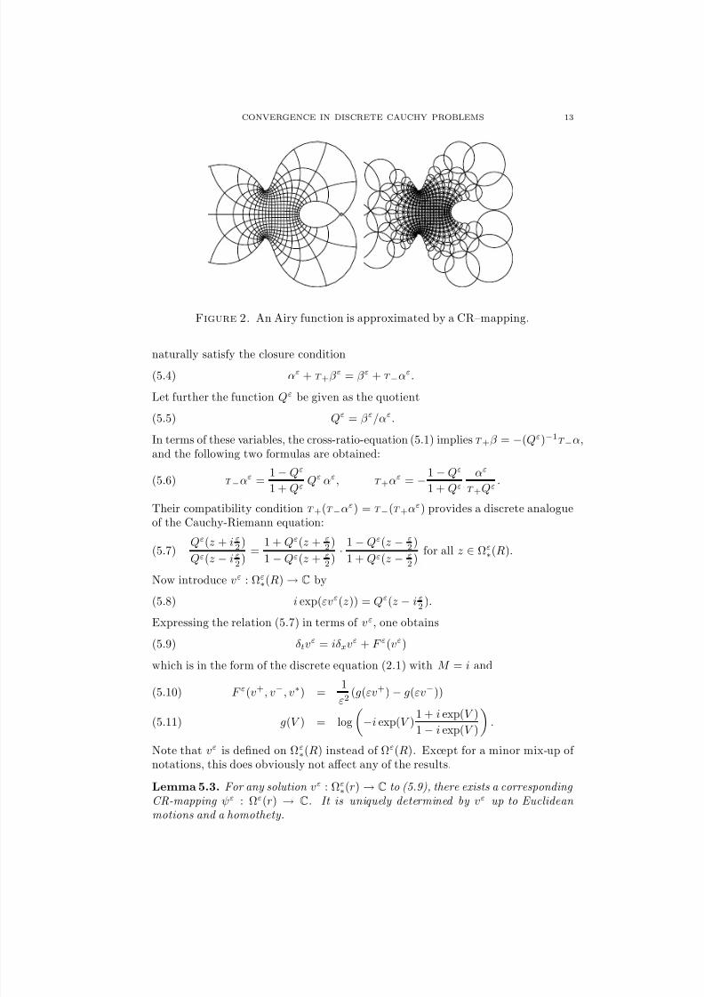
Figure 2. An Airy function is approximated by a CR–mapping.

naturally satisfy the closure condition

αε + T +β ε = β ε + T −αε.(5.4)

Let further the function Qε be given as the quotient

(5.5) Qε = β ε/αε.

In terms of these variables, the cross-ratio-equation (5.1) implies T +β = −(Qε)−1T −α,

and the following two formulas are obtained:

T −αε =1 − Qε

1 + QεQε αε, T +αε = −1 − Qε

1 + Qε

αε

T +Qε.(5.6)

Their compatibility condition T +(T −αε) = T −(T +αε) provides a discrete analogue

of the Cauchy-Riemann equation:Qε(z + i ε

2)

Qε(z − i ε2

)=

1 + Qε(z + ε2

)

1 − Qε(z + ε2

)· 1 − Qε(z − ε

2)

1 + Qε(z − ε2

)for all z ∈ Ωε

∗(R).(5.7)

Now introduce vε : Ωε∗(R) → C by

(5.8) i exp(εvε(z)) = Qε(z − i ε2

).

Expressing the relation (5.7) in terms of vε, one obtains

δtvε = iδxvε + F ε(vε)(5.9)

which is in the form of the discrete equation (2.1) with M = i and

F ε(v+, v−, v∗) =1

ε2(g(εv+)

−g(εv−))(5.10)

g(V ) = log

−i exp(V )

1 + i exp(V )

1 − i exp(V )

.(5.11)

Note that vε is defined on Ωε∗(R) instead of Ωε(R). Except for a minor mix-up of

notations, this does obviously not affect any of the results.

Lemma 5.3. For any solution vε : Ωε∗(r) → C to (5.9), there exists a corresponding

CR-mapping ψε : Ωε(r) → C. It is uniquely determined by vε up to Euclidean motions and a homothety.



14 D. MATTHES

Proof of Lemma 5.3. Let z be the “bottom” of Ωε(r), i.e., z = −irε ∈ Ωε(r) withr − ε

2 < rε ≤ r. Assign αε(z) an arbitrary, non-zero number Aε ∈ C. Equation

(5.8) defines Qε

from vε

, and (5.6) defines αε

on Ωε

(r). Consistency is provided,i.e. T +(T −αε) = T −(T +αε), because Qε solves (5.7). Let β ε = Qεαε. Assignan arbitrary number Ψε ∈ C to ψε(z), then define ψε on Ωε(r) according to (5.3).Compatibility (5.4) is guaranteed because αε solves (5.6). To verify that ψε is indeeda CR-mapping, combine equations (5.6) and (5.4). Variations of Aε correspond torigid rotations and dilations of the whole lattice ψε, variations of Ψε to translations.

Proof of Theorem 5.2, continued: The continuous counterpart of vε is

(5.12) u(z) = − 1

2

φ(z)

φ(z),

which is defined on some Ω(R) with R > 0 small enough (since φ(0)

= 0 by

hypothesis). To justify this ansatz, define

aε = (T +φ − φ)/ε, bε = (T −φ − φ)/ε(5.13)

as analogues of αε and β ε, respectively. By Taylor expansion, one finds

bε(z) = i exp(εu(z + i ε2

))aε(z) + O(ε2)(5.14)

T −aε(z) =1 − i exp(εu(z + i ε

2))

1 + i exp(εu(z + i ε2

))i exp(εu(z + i ε

2))aε(z) + O(ε2),(5.15)

corresponding to (5.5) and (5.6), respectively. The Cauchy-Riemann equation foru,

(5.16) ∂ tu = i∂ xu,

corresponds to M = i and f ≡ 0 in problem (1.1). Since g(0) = g

(0) = g

(0) = 0by (5.11), one easily verifies |F ε(v+, v−, v∗)| ≤ Kε|v+ − v−|, so the function F ε in(5.10) satisfies the estimate (2.2). Let vε be the solution to (5.9) with initial data(2.3) obtained from the function u in (5.12). Theorem 2.2 yields approximation of u by vε, according to estimate (2.4).By Lemma 5.3, vε corresponds to a CR-mapping ψε. Fix ψε by choosing ψε(z) =φ(z) and αε(z) = (T +φ(z)− φ(z))/ε. It remains to be shown that approximation of u by vε implies approximation of φ by ψε. Smooth approximation is again provenwith the help of suitable norms, which are in this case

wε(N ) =

m+n≤N

1

m!n!max

z∈Ωεm+n(r)

|δmx δnt wε(z)|.(5.17)

This norm is submultiplicative, so Lemma 3.2 applies. The other essential ingredi-

ent is

Lemma 5.4. For v : Ωε(r) → Cd, and N ≥ 0, one has

v(N +1) ≤ C r(|v(z1)| + |v(z2)| + δxv(N ) + δtv(N )),(5.18)

where z1, z2 ∈ Ωε(r) are arbitrary points with 0 < |z1 − z2| < ε.

Proof of Lemma 5.4. From the definition, it is clear that

v(N +1) ≤ maxz∈Ωε(r)

|v(z)| + δxv(N ) + δtv(N ).




Write z1 = (t1, x1), z2 = (t2, x2) and let z = (t, x) ∈ Ωε(r) be arbitrary. Thereexist integers P and Q with t = ti + εP and x = xi + εQ for either i = 1 or i = 2.

Naturally, ε|P | + ε|Q| ≤ 2r. Thus

|v(z)| ≤ |v(zi)| + εP

p=1

|δxv(zi + pε − ε2

)| + ε

Qq=1

|δtv(z − iqε + i ε2

)|

≤ |v(zi)| + 2r(δxv(N ) + δtv(N )).

So (5.18) holds with C r = 1 + 2r.

Proof of Theorem 5.2, continued: At this point, it is sensible to introduce thenotion uε = O∞(ε p) for a family of smooth functions uε : Ω(r) → C

d, meaning thatuεC N (Ω) < C N ε p for all N ≥ 0, with suitable constants C N > 0.

Lemma 5.5. Let u : Ω(r) → Cd be an arbitrary smooth function. For natural

numbers m, n, one has(5.19) [∂ mx ∂ nt u]ε = δmx δnt [u]ε + O∞(ε2).

Moreover, for λx, λt ∈ R, define uε±(x, t) = u(x ± ελx, t ± ελt). Then

uε+ + uε

− = 2u + O∞(ε2),(5.20)

uε+ − uε

− = 2ε(λx∂ xu + λt∂ tu) + O∞(ε3).(5.21)

The identity (5.19) is proven in the appendix. The derivation of the properties(5.20), (5.21) is analogous.It is clear from Theorem 2.2 and Lemma 5.5 that [u]ε−vε(N ) = O(ε2) for arbitraryN . It is now shown that this implies

αε − aε(N ) = O(ε2).(5.22)

Introduce the functions gε, Gε by

(5.23) α(z) = exp(gε(z))α(z), a(z) = exp(Gε(z))a(z).

Combining the formulas in (5.6) yields the simple relation

τ xαε = T −1− (T +αε) =

−1

(τ xQε)(T −1− Qε)

αε, so δxgε = −(T +vε + vε).

Adopting the notion O∞(ε2), and using the rules (5.20) and (5.21),

∂ xGε(z) =T +φ − φ

T +φ − φ(z) =

φ

φ(z + 1+i

2ε2

) + O∞(ε2)

= −2u(z + 1+i2

ε2

) + O∞(ε2) = −(T +u + u)(z) + O∞(ε2).

Similar identities are derived for δtgε and ∂ tGε, so that

δx(gε − Gε)(N ) + δt(gε − Gε)(N ) ≤ 4[u]ε − vε(N ) + O(ε2) = O(ε2).

As αε(z) = aε(z) by construction, the asymptotic estimates (5.14), (5.15) yieldT −αε(z) = T −aε(z) + O(ε2). Hence also gε(z) = Gε(z) = 0 a n d T −gε(z) =T −Gε(z) + O(ε2). Lemma 5.4 gives

Gε − gε(N ) ≤ C N [u]ε − vε(N ).

By means of the composition estimate (3.8),

αε − aε(N ) ≤ exp(gε) − exp(Gε)(N ) |α(z)| = O(ε2),



16 D. MATTHES

and this implies (5.22). An analogous argument gives the respective approximationof bε by β ε.

In the second step, ψε

and φ are reconstructed from αε

, β ε

and aε

, bε

, respectively.By definition of these quantities,

δxψε(z) = αε(z − ε2 ) − β ε(z + ε

2 ), δx[φ]ε(z) = aε(z − ε2 ) − bε(z + ε

2 ),

δtψε(z) = αε(z − i ε

2) + β ε(z + ε

2), δt[φ]ε(z) = aε(z − i ε

2) + bε(z + ε

2).

By construction of ψε, one has ψε(z) = φ(z), and also T +ψε(z) = T +φ(z) + O(ε2)because αε(z) = aε(z) + O(ε2). Applying Lemma 5.4 to [φ]ε and ψε gives [φ]ε −ψε(N ) = O(ε2) and thus the desired final result (5.2).

6. Schramm’s Orthogonal Patterns

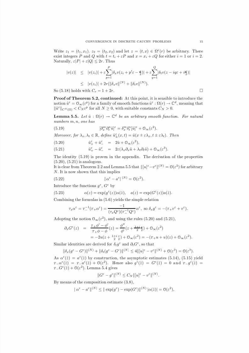
In [Sch], Schramm-patterns (or orthogonal circle patterns) are proposed as discreteanalogues of conformal maps. A Schramm-pattern Cε assigns to each vertex (x, t)

∈Ωε ⊂ (εZ)2 a circle Cε(x, t) in R2 ≡ C. The defining condition is that circles

belonging to neighboring vertices intersect orthogonally, and circles assigned toopposite corners of an (εZ)2-square are tangent. So Cε(x, t) and Cε(x, t) intersectorthogonally and are tangent, respectively, if |x − x| + |t − t| = ε and if |x − x| =|t − t| = ε. For the formal definition, refer to the original article.The theory developed here allows for an easy proof of local C ∞-approximation of conformal maps. The obtained local result differs in nature from the C 0-convergencetheorem presented in [Sch], which deals with global boundary value problems.For notational simplicity, the domain for an orthogonal circle pattern Cε is

Ωε(r) = Ωε(r) ∩ (εZ)2,

containing half of the grid points of Ωε(r). In obvious analogy to Ωεk(r), the sets

Ωεmn(r) ⊂ Ωεm+n(r) are introduced so that the central difference quotient δmx δnt ψε

of a function ψε on Ωε(r) is naturally evaluated on Ωεmn(r). Note that Ωε

mn and

Ωεnm do not coincide in general.

Figure 3. An Airy function is approximated by a Schramm-pattern.

By the results in [Sch], a pattern Cε is – up to rigid motions – determined by itsradius function ρε, which assigns to each point (t, x) ∈ (εZ)2 the radius of the circleCε(t, x).




Theorem 6.1. Given a conformal map φ : Ω(R) → C with ∂ xφ(0) = 0, there isa positive r < R, and there exists a family of orthogonal circle patterns Cε defined

on Ωε

(r) for all ε > 0 small enough, whose radii functions ρε

are convergent to themetric factor ρ = |∂ xφ| of φ in C ∞,

sup(x,t)∈Ωε

mn(r)

|δmx δnt ρε(x, t) − ∂ mx ∂ nt ρ(x, t)| ≤ C mnε2.(6.1)

Proof. The function log ρ is harmonic, i.e., satisfies Laplace’s equation

∂ 2x(log ρ) + ∂ 2t (log ρ) = 0.(6.2)

In terms of u(1) = ∂ x(log ρ) and u(2) = ∂ t(log ρ), harmonicity reads

∂ t

u(1)

u(2)

=

0 1

−1 0

∂ x

u(1)

u(2)

.(6.3)

For the radius function ρε of a Schramm-pattern, an “exponential Laplace equation”

has been derived in [Sch]. In our notations,(6.4)

(τ 2xρε)(τ 2t ρε)(τ −2x ρε)(τ −2

t ρε)

(ρε)2=

(τ 2xρε) + (τ 2t ρε) + (τ −2x ρε) + (τ −2

t ρε)

(τ 2xρε)−1 + (τ 2t ρε)−1 + (τ −2x ρε)−1 + (τ −2

t ρε)−1.

Recall that τ x and τ t denote the ε2

-shift in the x- and t-direction, respectively, so

that τ ±2x and τ ±2

t are shifts by ε. Equation (6.4) is satisfied by a positive function

ρε : Ωε(r) → R+ if and only if it is the radius function of a Schramm-pattern.Introduce functions vε(1), vε(2) by

exp(εvε(1)) = (τ xρε)/(τ −1x ρε), exp(εvε(2)) = (τ tρε)/(τ −1

t ρε).(6.5)

Since ρε is given on Ωε(r), vε(1) and vε(2) are a priori defined on different subsets of

Ωε∗(r). However, the domains of the difference quotients δtv

ε(1) and δxv

ε(2) coincide,

and the same is true for δxvε(1) and δtvε(2). Equation (6.4) and the compatibility

condition δxvε(2) = δtvε(1) imply formally

δt

vε(1)

vε(2)

=

0 1

−1 0

δx

vε(1)

vε(2)

+

0

Gε

,(6.6)

with Gε = 1ε2 log(H ε/H −ε)

H ε(v+, v−, v∗) = eεv+(1) + e−εv−

(1) + e−εv∗(2) − eε(v+(1)−v−(1)−v∗(2)).

Suppose vε : Ωε∗(r) → R2 is a solution to (6.6), then the equations (6.5) are com-

patible. From the components vε(1) and vε(2), a solution ρε : Ωε(r) → R+ to (6.5)

can be constructed and is uniquely determined up to a global scalar factor. (Notethat vε(1) and vε(2) are defined at more points than needed to calculate ρε. Actually,

any solution vε to (6.6) corresponds to two independent Schramm-pattern.) ρε sat-isfies the exponential Laplace equation (6.4), hence is the radius function of some

Schramm-pattern Cε on Ωε(r).H is an analytic function with respect to v+, v−, v∗ and ε. Keeping the values of the v’s fixed, a simple calculation shows that

d

dε

kε=0

log(H ε/H −ε) =

0 for k = 0, 1, 2

(v+(1)

− v−(1)

) · h(v) for k = 3,



18 D. MATTHES

where h is some analytic expression of the v’s. Hence |Gε| ≤ Kε|v+ −v−|, implyingthe estimate (2.2) for F . Now let vε be the solution to (6.6) with the restrictions

of u as initial data in (2.3). Theorem 2.2 applies and yields convergence of vε

to uon a suitable Ω(r).Make the respective solution ρε of (6.5) unique by choosing ρε(0, 0) = ρ(0, 0).From estimates completely analogous to those used in the proof of Theorem 5.2(reconstruction of αε from vε) one obtains C ∞-convergence of ρε to ρ.

The radius function ρε : Ωε(r) → R+ is accompanied by a function ψε : Ωε(r) → C,such that Cε(x, t) is the circle of radius ρε(x, t) > 0 around the center ψε(x, t) ∈ C.

Theorem 6.2. Under the hypotheses of Theorem 6.1 and for every ε > 0 small enough, there exists a Schramm-pattern Cε on Ωε(r), such that the circle centersψε converge to the conformal map φ in C ∞:

sup

(x,t)∈Ωεmn(r) |δmx δnt ψε(x, t)

−∂ mx ∂ nt φ(x, t)

| ≤C mnε2.(6.7)

Proof. As pointed out before, the radius function alone determines the pattern Cε

– and hence ψε – up to a rigid motion. Formulas for the reconstruction of φ andψε from ρ and ρε, respectively, are now derived.Introduce the real-valued function ω on Ω(R) by

(6.8) φ = ρ exp(iω),

where φ(x, t) := ∂ xφ(x, t) is holomorphic with respect to the complex variablez = x + it. The Cauchy-Riemann equations for φ read

∂ xω = −∂ t log ρ = −u(2)(6.9)

∂ tω = ∂ x log ρ = u(1),(6.10)

with u defined as before, u(1) = ∂ x(log ρ), u(2) = ∂ t(log ρ).Analogous quantities and relations are now given for an arbitrary Schramm-patternCε. Define the real functions ωε and dε on Ωε

1,0(r) by

δxψε = dε exp(iωε),(6.11)

with dε(x, t) denoting the euclidian distance between the circle centers ψε(x + ε2

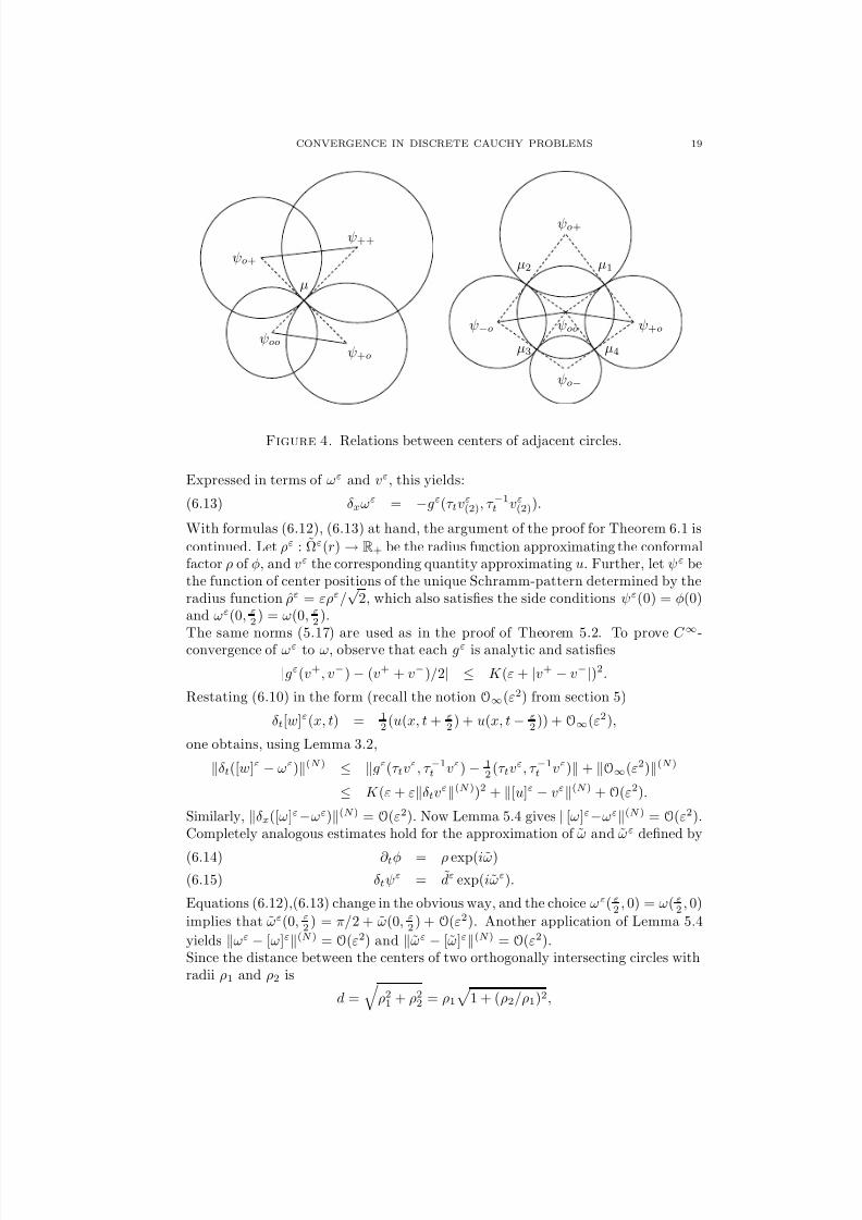
, t)and ψε(x + ε

2 , t), and ωε(x, t) the slope of their connecting line to the x-axis.In Fig. 4, two pieces of a Schramm-pattern are displayed. From the left sketch, itis clear that

∠(ψ++ − ψ0+, ψ+0 − ψ00) = ∠(µ, ψ0+, ψ++) −∠(ψ00, ψ+0, µ)

= arctan

ρ++

ρ0+ − arctan

ρ00

ρ+0.

Introducing vε by the formulas (6.5),

δtωε = gε(τ tvε(1), τ −1t vε(1))(6.12)

gε(v+, v−) = 1ε

arctanexp(εv+) − arctanexp(−εv−)

.

From the sketch on the right, it follows that

∠(ψ+0 − ψ00, ψ00 − ψ−0) = ∠(µ4, ψ00, µ3) − ∠(µ1, ψ00, µ2)

= arctan

ρ0−

ρ00

− arctan

ρ0+

ρ00

.




ψooψ+o

ψo+

ψ++

µ

ψooψ−o ψ+o

ψo−

ψo+

µ1µ2

µ3 µ4

Figure 4. Relations between centers of adjacent circles.

Expressed in terms of ωε and vε, this yields:

δxωε = −gε(τ tvε(2), τ −1t vε(2)).(6.13)

With formulas (6.12), (6.13) at hand, the argument of the proof for Theorem 6.1 is

continued. Let ρε : Ωε(r) → R+ be the radius function approximating the conformalfactor ρ of φ, and vε the corresponding quantity approximating u. Further, let ψε bethe function of center positions of the unique Schramm-pattern determined by theradius function ρε = ερε/

√2, which also satisfies the side conditions ψε(0) = φ(0)

and ωε(0, ε2

) = ω(0, ε2

).The same norms (5.17) are used as in the proof of Theorem 5.2. To prove C ∞-convergence of ωε to ω, observe that each gε is analytic and satisfies

|gε(v+, v−) − (v+ + v−)/2| ≤ K (ε + |v+ − v−|)2.

Restating (6.10) in the form (recall the notion O∞(ε2) from section 5)

δt[w]ε(x, t) = 12

(u(x, t + ε2

) + u(x, t − ε2

)) + O∞(ε2),

one obtains, using Lemma 3.2,

δt([w]ε − ωε)(N ) ≤ gε(τ tvε, τ −1t vε) − 1

2(τ tvε, τ −1

t vε) + O∞(ε2)(N )

≤ K (ε + εδtvε(N ))2 + [u]ε − vε(N ) + O(ε2).

Similarly, δx([ω]ε−ωε)(N ) = O(ε2). Now Lemma 5.4 gives [ω]ε−ωε(N ) = O(ε2).Completely analogous estimates hold for the approximation of ω and ωε defined by

∂ tφ = ρ exp(iω)(6.14)

δtψε = dε exp(iωε).(6.15)

Equations (6.12),(6.13) change in the obvious way, and the choice ωε( ε2

, 0) = ω( ε2

, 0)

implies that ωε(0, ε2

) = π/2 + ω(0, ε2

) + O(ε2). Another application of Lemma 5.4

yields ωε − [ω]ε(N ) = O(ε2) and ωε − [ω]ε(N ) = O(ε2).Since the distance between the centers of two orthogonally intersecting circles withradii ρ1 and ρ2 is

d =

ρ21 + ρ2

2 = ρ1

1 + (ρ2/ρ1)2,



20 D. MATTHES

the quantities dε and dε are given by

dε

= 1+exp(2εvε(1))

2 (τ −1x ρ

ε

), dε

= 1+exp(2εvε(2))

2 (τ −1

t ρε

).(6.16)Now observe that1

ρ =

ρ2 =

τ −1x ρ2+τ xρ

2

2+ O∞(ε2) =

1+(τ xρ/τ

−1x ρ)2

2(τ −1

x ρ) + O∞(ε2)

=

1+exp(2εu(1))

2 (τ −1x ρ) + O∞(ε2).

Hence, with Lemma 3.2 it follows

δx(ψε − [φ]ε)(N ) ≤ C N (ρε − [ρ]ε(N ) + ωε − [ω]ε(N )) + O(ε2),

δt(ψε − [φ]ε)(N ) ≤ C N (ρε − [ρ]ε(N ) + ωε − [ω]ε(N )) + O(ε2).

An application of Lemma 5.4 finishes the argument.

7. Appendix

Proof of Lemma 3.1. As a finite sum of norms, · ρ is seen to constitute a normitself. The absolute bound is trivial.Submultiplicativity: For two functions u, v : Iεn → C,

uvρ =n

k=0

ρk

k!sup

x∈Iεn−k

|δkx(uv)(x)|

≤k≤n

ρk

k!

k=0

k

sup

x∈Iεn−

|δxu(x)| supy∈Iε

n−k+

|δk−x v(y)|

≤

n

=0

n

m=0

ρ+m

! m!sup

x∈Iεn− |δ

x

u(x)|

supy∈Iεn−m |

δm

x

v(y)|

≤ uρvρ.

Discrete Cauchy estimate: For u : Iεn → Cd,

uρ + θδxuρ =n

k=0

ρk

k!max

x∈Iεn−k

|δkxu(x)| + θn−1k=0

ρk

k!max

x∈Iεn−k−1

|δk+1x u(x)|

≤n

k=0

ρk

k!(1 + θ

k

ρ) maxx∈Iε

n−k

|δkxu(x)|

≤n+1

k=0

(ρ + θ)k

k!max

x∈Iεn−k

|δkxu(x)| = uρ+θ

because for k = 0, 1, . . ., one has 1 + kθ/ρ ≤ (1 + θ/ρ)k.Restriction estimate: With the classical Cauchy estimate

supx∈I

|∂ kxu(x)| ≤ k!(1/ρ)k supx∈Bρ(I)

|u(x)|

1The reason formulas (6.16) are employed instead of the symmetric representation d =q ρ2

1 + ρ22 is that the former is an analytic expression in ρ, u on some D(U ) with arbitrarily

large U as ε→ 0, whereas the latter has a singularity at ρ1 = ρ2 = 0.




it follows that

[u]ερ =

nk=0

ρ

k

k! supx∈Iε

n−k

|δkx[u]ε(x)| ≤n

k=0

ρ

k

k! supx∈I

|∂ kxu(x)|

≤

nk=0

(ρ/ρ)k

sup

x∈Bρ (I)|u(x)|.

Analyticity estimate: For simplicity, assume that all nε are odd. vερ ≤ C implies|δsvε(x)| ≤ Cs!ρ−s for all x ∈ Iεnε and all s ≤ nε. Hence, for fixed s ≥ 0 and εsmall enough, the sequence of interpolated functions Eδs

xvε is equicontinuous.At s = 0, the Arzel‘a-Ascoli theorem yields a subsequence ε(0) → 0 of ε so thatEvε(0) converges uniformly to a continuous function u. From here, proceed in-ductively: Assume that Eδsxvε(s) converges uniformly to ∂ sxu. Apply the Arzel‘a-Ascoli theorem at s + 1 to obtain an infinite subsequence ε(s + 1) of ε(s) for which

Eδs+1x vε(s+1) converges uniformly to some u(s+1). To show that u(s+1) is indeedthe s + 1-st derivative of u, consider the identity

(δsxuε(s+1))(x) = (δsxuε(s+1))(0) + ε

0≤j<J

(δs+1x uε(s+1))( ε

2+ εj)

with arbitrary x = εJ ∈ Iεnε−s. This implies for the interpolated functions

(Eδsxuε(s+1))(x) = (Eδsxuε(s+1))(0) +

x0

(Eδs+1x uε(s+1))(z) dz + O(ε)

at arbitrary x ∈ I. Pass to the limit ε → 0 on both sides. u(s+1) is seen to be thex-derivative of ∂ sxu, so u

∈C s(I). From the theorem on dominated convergence, it

follows for x ∈ I ∞s=0

ρs

s! |∂ sxu(x)| ≤ C.

So u possesses a convergent Taylor expansion around all x ∈ I, with convergenceradius ρ, and the analytic extension is bounded by C .

Proof of Lemma 3.2. As |u(i)(ξ)| ≤ uρ < U/γ by hypothesis and property (1),the composition g(u) is a well-defined function on the respective Iεn. The estimate(3.6) is derived as follows: Since g : D p(U ) → C

d is analytic, it has a power seriesrepresentation

g(u) = α∈Np0

∂ αg(0)

α! uα

, uα

= p

j=1 uαjj ,(7.1)

where α = (α1, . . . , α p) denotes a multi-index. For the coefficients in (7.1), theCauchy integral representation yields

|∂ αg(0)|α!

=1

(2π) p

|µ1|=m1

dµ1 · · · |µp|=mp

dµ pg(µ1, . . . , µ p)

µα1+11 · · · µ

αp+1 p

≤ F (m1, . . . , m p)

mα11 · · · m

αp p

,



22 D. MATTHES

the mi being arbitrary numbers with 0 < mi < U . Choosing mi = γ u(i)ρ, itfollows from submultiplicativity and the basic norm properties of · ρ that

g(u)ρ ≤ α

∂ αg(0)α!

uαρ

≤ F (m1, . . . , m p)

α

u(1)ρm1

α1 · · ·u(p)ρmp

αp≤

αγ −|α| · F (γ u(1)ρ, . . . , γ u( p)ρ).

This proves the claim and also shows that Γ := (1 − 1/γ )− p is independent of thenorm · ρ.

Proof of Lemma 5.5. One starts with the representation

δmx δnt [u]ε(x, t) =1

εm+n [−ε2 ,+

ε2 ]

m

dmξ

[−ε2 ,+

ε2 ]n

dnτ ∂ mx ∂ nt u(x + ξ, t + τ )

of arbitrary partial difference quotients, where ξ= (ξ1, . . . , ξm) τ = (τ 1, . . . , τ n) andthe notations ξ =

mi=1 ξi and τ =

nj=1 τ j have been used. Then,

(δmx δnt [u]ε − ∂ mx ∂ nt u)(x, t) =

dξ dη

εm+n

10

ds ∂ (ξτ )∂ mx ∂ nt u(x + sξ, t + sτ )

=

dξ dη

εm+n

10

ds

∂ (ξτ )∂ mx ∂ nt u(x, t) A(x,t)

+s 1

0ds ∂ 2(ξτ )∂ mx ∂ nt u(x + ssξ, t + ssτ )

B(x,t)

.

Above, ∂ (ξτ ) = (ξ)∂ x + (τ )∂ t. The integral over A vanishes because

dmξ

dnτ ∂ (ξτ )f = 0

for an arbitrary ξ, τ -independent function f . As B(x, t) is an (x, t)-smooth func-tion, one concludes (5.19).

References

[BMS] A.I. Bobenko, D. Matthes, Yu.B. Suris Discrete and smooth orthogonal systems: C ∞-

approximation. Int. Math. Res. Not. 45 (2003), 2415–2459.[BP1] A.I. Bobenko, U. Pinkall, Discrete isothermic surfaces, J. Reine Angew. Math. 475 (1996),

187–208.[BP2] A.I. Bobenko, U. Pinkall Discretization of surfaces and integrable systems. in: “Discrete in-

tegrable geometry and physics” (Vienna, 1996), Oxford Lecture Ser. Math. Appl., 16, OxfordUniv. Press, New York, 1999.

[DHR] P. Doyle, Z.X. He, B. Rodin Second derivatives of circle packings and conformal mappings.

Discrete Comput. Geom. 11 (1994), no. 1, 35–49.[HS] Z.X. He, O. Schramm The C ∞-convergence of hexagonal disk packings to the Riemann map.

Acta Math. 180 (1998), no. 2, 219–245.[Nag] M. Nagumo ¨ Uber das Anfangswertproblem partieller Differentialgleichungen. Jap. J. Math.

18, (1942). 41–47.[Nir] L. Nirenberg An abstract form of the nonlinear Cauchy-Kowalewski theorem. J. Differential

Geometry 6 (1972), 561–576.[NQC] F.W. Nijhoff, G.R. Quispel, H.W. Capel Direct linearization of nonlinear difference-

difference equations. Phys. Lett. A 97 (1983), no. 4, 125–128.

[RS] B. Rodin, D. Sullivan The convergence of circle packings to the Riemann mapping. J. Dif-ferential Geom. 26 (1987), no. 2, 349–360.

[Sch] O. Schramm Circle patterns with the combinatorics of the square grid. Duke Math. J. 86(1997), no. 2, 347–389.




[Wal] W. Walter An elementary proof of the Cauchy-Kowalevsky theorem. Amer. Math. Monthly92 (1985), no. 2, 115–126.

E-mail address:[email protected]

Institut fur Mathematik, Johannes Gutenberg Universitat Mainz, Staudingerweg 9,

55128 Mainz, Germany.

d.matthes- convergence in discrete cauchy problems and applications to circle patterns

Documents