diversity selective fading channels - mins.ee.ethz.ch · résumé la plupart des nouvelles...
TRANSCRIPT

DIVERSITY-MULTIPLEXING TRADEOFF IN
SELECTIVE-FADING CHANNELS


Pedro E. Coronel
DIVERSITY-MULTIPLEXINGTRADEOFF IN SELECTIVE-FADING
CHANNELS
Hartung-Gorre Verlag Konstanz2009

Reprint of Diss. ETH No. 17896
SERIES IN COMMUNICATION THEORY VOLUME 5
edited by Helmut Bölcskei
Bibliographic Information published by Die Deutsche Bibliothek
Die Deutsche Bibliothek lists this publication in the DeutscheNationalbibliografie; detailed bibliographic data is available athttp://dnb.ddb.de.
Copyright © 2009 by Pedro E. Coronel
First edition 2009
HARTUNG-GORRE VERLAG KONSTANZ
ISSN 1865-6765ISBN-10 3-86628-251-6ISBN-13 978-3-86628-251-3

A mi querida familia


Abstract
Recent years have seen the proliferation of new wireless data applica-tions that have fueled the demand for communication systems capableof delivering very high quality-of-service (QoS) in terms of data rateand reliability. At the same time, due to the surge in the number ofwireless devices, the spectrum available for communication has becomescarcer, and the level of interference has increased significantly. Thedesign of systems satisfying stringent QoS requirements is therefore aparticularly challenging task that requires an accurate understandingof the ultimate performance of communication over wireless channels.In this thesis, we establish information-theoretic limits on rate andreliability in wireless communication, and we provide guidelines todesign systems that achieve these limits.
Rate and reliability are two essential properties of communicationsystems that are subject to tension: increasing data rate typically resultsin larger error probability and, conversely, a reduction in error prob-ability often comes at the price of sacrificing data rate. The balancethat a system is able to strike between rate and reliability providesa comprehensive view of its performance. Unfortunately, a precisecharacterization of the rate-reliability tradeoff is difficult in general.In fading channels, however, the diversity-multiplexing (DM) tradeoffframework proposed by Zheng and Tse (2003) has proved to be veryhelpful in understanding the interplay between rate and reliability inthe high signal-to-noise ratio (SNR) regime. The analysis conducted in
vii

this thesis adopts this framework and uses the notions of diversity andmultiplexing to capture, respectively, the reliability and data rate of thesystem.
In many situations of practical relevance, the wireless channel ex-hibits time and frequency selectivity arising from temporal variations inthe environment and multipath propagation. A direct characterization ofthe DM tradeoff in this class of channels, referred to as selective-fadingchannels, is in general difficult because the corresponding mutual infor-mation is a sum of correlated random variables. This thesis presents atechnique that bypasses this difficulty and establishes the optimal DMtradeoff of selective-fading channels in both the point-to-point case andthe multiple-access (MA) case. The essence of our approach is to studythe “Jensen channel” that is associated with the original channel andthat has the same behavior in the regime of high SNR relevant to theDM tradeoff framework.
In the point-to-point case, we obtain a code design criterion thatguarantees optimal performance in the sense of the DM tradeoff and thatties in nicely with several code design criteria reported in prior work.The systematic construction of optimal codes is nontrivial when thetransmitter is equipped with multiple antennas. We show, however, thatthe design problem can be separated into two simpler and independentproblems: the design of an inner code, also referred to as precoder,adapted to the selectivity characteristics of the channel, and the designof an outer code which, quite remarkably, is independent of the channelcharacteristics.
Our investigation of selective-fading MA channels yields a detailedcharacterization of the limitations that multiuser interference puts onoptimal performance. In particular, we find an interesting conceptualrelation between the DM tradeoff framework and the notion of domi-nant error event, which was first introduced in additive white Gaussiannoise (AWGN) channels by Gallager (1985). Studying the dominanterror event as a function of the users’ rates reveals the existence ofoperational regimes in which multiuser interference has only a negli-
viii

gible impact on error performance. As in the point-to-point case, weobtain a set of code design criteria that guarantees optimal performanceto all users. The construction of optimal codes is nontrivial and re-quires the users to jointly design their codes. We finally examine a codeconstruction which satisfies our criteria for the two-user flat-fadingchannel.
ix


Résumé
La plupart des nouvelles applications sans fil exigent des systèmes decommunication assurant une haute qualité de service (QoS) mesuréeen termes de débit et de fiabilité. Cependant, l’augmentation rapidedu nombre de ces systèmes se heurte à la difficulté de trouver desfréquences disponibles dans les bandes spectrales réglementaires. Desutilisateurs de plus en plus nombreux doivent se partager des bandesspectrales dont la largeur n’augmente pas et les systèmes de com-munication sous-jacents sont confrontés à une élévation du niveaud’interférence. Dès lors, la conception de systèmes de communicationsans fil offrant une QoS élevée nécessite une compréhension appro-fondie des limites fondamentales qui régissent leur performance. Cettethèse vise tout d’abord à établir certaines de ces limites en utilisant lathéorie de l’information. Elle présente aussi des critères permettant laconstruction de codes capables d’atteindre une performance optimale.
Le débit de transmission et la fiabilité sont deux paramètres essentielset antagonistes d’un système de communication: une augmentationdu débit entraine généralement plus d’erreurs et, inversement, uneamélioration de la fiabilité se traduit souvent par une diminution dudébit. La performance d’un système se caractérise intégralement par lecompromis qu’il est capable de réaliser entre débit et fiabilité. Mais ilest souvent difficile de déterminer ce compromis avec précision. Dansle cas des canaux à évanouissements, le cadre théorique du compromisdiversité-multiplexage (DM) introduit par Zheng and Tse (2003) permet
xi

de quantifier l’antagonisme entre débit et fiabilité lorsque le rapportsignal sur bruit (SNR) est élevé. L’analyse développée dans cette thèses’inscrit dans ce cadre et utilise en particulier les notions de diversité etde multiplexage pour rendre compte respectivement de la fiabilité et dudébit du système.
Dans la pratique, le canal sans fil est souvent sélectif en fréquence eten temps en raison de variations temporelles de l’environnement et dela propagation par trajets multiples. En général, le compromis DM descanaux sélectifs est difficile à déterminer car l’information mutuellecorrespondante est une somme de variables aléatoires corrélées. Cettethèse introduit une méthode qui contourne cette difficulté et qui permetd’établir le compromis DM optimal pour les canaux sélectifs point-à-point et à accès multiple (MA). Notre approche consiste à étudierle “canal de Jensen” qui est associé au canal sans fil original et qui secomporte de façon similaire dans le régime de grand SNR, c’est-à-diredans le régime qui est pertinent du point de vue du compromis DM.
Dans le cas des canaux point-à-point, nous obtenons un critère pourla construction de codes optimaux dans le sense du compromis DM. Deplus, nous montrons que notre critère est cohérent avec d’autres critèresénoncés dans des travaux antérieurs. La construction systématique decodes optimaux devient un problème complexe lorsque le transmetteurest équipé de multiples antennes. Cependant, nos résultats démontrentqu’une telle tâche peut être décomposée en deux opérations plus sim-ples et indépendantes: d’une part, la construction d’un code interne, ou“précodeur”, développé en fonction des statistiques du canal, et d’autrepart, la conception d’un code externe qui est indépendant du canal.
Notre étude des canaux sélectifs à MA fournit une caractérisationdétaillée de la manière dont l’interférence entre utilisateurs affectela performance optimale. En particulier, nous trouvons une relationconceptuelle intéressante entre le compromis DM et la notion d’erreurdominante introduite dans le cadre des canaux à bruit additif gaussienpar Gallager (1985). Nos résultats révèlent qu’en fonction des débitsdes utilisateurs, l’interférence peut parfois n’avoir qu’une influence
xii

négligeable sur la probabilité d’erreur. Comme dans le cas des lienspoint-à-point, nous obtenons un ensemble de critères pour construiredes codes distribués qui atteignent la performance optimale. Nousexaminons finalement un exemple de code distribué qui satisfait noscritères dans le cas d’un canal non-sélectif avec deux utilisateurs.
xiii


Acknowledgments
I thank Prof. Helmut Bölcskei for his constant support during the devel-opment of this dissertation. I also thank my manager at the IBM ZurichResearch Laboratory, Dr. Pierre Chevillat, for his trust and support. Fur-thermore, I would like to express my gratitude to Dr. Wolfgang Schottfor being an exceptional mentor throughout my IBM PhD fellowship.
I am very much indebted to all my friends and colleagues at ETHZurich and at the IBM Zurich Research Laboratory for making myresearch truly interesting and enjoyable. For their help and invalu-able input to my work, my very special thanks go to Cemal Akçaba,Dr. Simeon Furrer, Dr. Markus Gärtner, Dr. Ateet Kapur, Patrick Kup-pinger, Dr. Ulrich Schuster, and Beat Weiss.
My final word of gratitude goes to my family and friends for theirpatience and care. They have been a priceless source of inspiration andhelp during all these years.
xv


Contents
Acknowledgments xv
1 Introduction 11.1 Motivation . . . . . . . . . . . . . . . . . . . . . . . . 11.2 Outline . . . . . . . . . . . . . . . . . . . . . . . . . 3
2 The Selective-Fading Channel 72.1 The underspread fading channel . . . . . . . . . . . . 9
2.1.1 Stochastic model . . . . . . . . . . . . . . . . 102.1.2 The underspread assumption . . . . . . . . . . 112.1.3 Approximate diagonalization . . . . . . . . . . 112.1.4 Canonical signaling scheme . . . . . . . . . . 13
2.2 System model . . . . . . . . . . . . . . . . . . . . . . 14
3 The Diversity-Multiplexing Tradeoff 193.1 Preliminaries . . . . . . . . . . . . . . . . . . . . . . 20
3.1.1 Rate and multiplexing . . . . . . . . . . . . . 203.1.2 Reliability and diversity . . . . . . . . . . . . 213.1.3 System definitions . . . . . . . . . . . . . . . 22
3.2 Performance limits . . . . . . . . . . . . . . . . . . . 233.2.1 Outage probability . . . . . . . . . . . . . . . 243.2.2 Performance bound . . . . . . . . . . . . . . . 253.2.3 Achievability . . . . . . . . . . . . . . . . . . 27
xvii

CONTENTS
3.3 Evaluation of the outage probability . . . . . . . . . . 293.3.1 Geometric interpretation . . . . . . . . . . . . 323.3.2 Visualization of the tradeoff . . . . . . . . . . 33
3.4 Multiple-access channel . . . . . . . . . . . . . . . . . 353.4.1 Achievable rate regions . . . . . . . . . . . . . 353.4.2 Multiple-access system definitions . . . . . . . 383.4.3 Outage formulation . . . . . . . . . . . . . . . 39
3.5 Beyond flat fading . . . . . . . . . . . . . . . . . . . . 42
4 Performance Limits in Selective-Fading Channels 434.1 Signal and channel model . . . . . . . . . . . . . . . . 444.2 Problem formulation . . . . . . . . . . . . . . . . . . 464.3 Analysis tool . . . . . . . . . . . . . . . . . . . . . . 51
4.3.1 The Jensen channel . . . . . . . . . . . . . . . 514.3.2 The Jensen outage probability . . . . . . . . . 52
4.4 Optimal DM tradeoff . . . . . . . . . . . . . . . . . . 564.4.1 Code design criterion . . . . . . . . . . . . . . 564.4.2 Geometric interpretation . . . . . . . . . . . . 644.4.3 Selectivity and optimal performance . . . . . . 66
4.5 Relation to other design criteria . . . . . . . . . . . . . 684.5.1 Non-vanishing determinant . . . . . . . . . . . 684.5.2 Approximate universality . . . . . . . . . . . . 694.5.3 Classical space-time code design criteria . . . 704.5.4 A geometric view on code design . . . . . . . 72
5 Optimal Code Construction 755.1 Single transmit antenna . . . . . . . . . . . . . . . . . 765.2 Multiple transmit antennas . . . . . . . . . . . . . . . 79
5.2.1 Preliminaries . . . . . . . . . . . . . . . . . . 795.2.2 Precoding setup . . . . . . . . . . . . . . . . . 805.2.3 Design criteria with precoding . . . . . . . . . 825.2.4 Outer family of codes . . . . . . . . . . . . . . 85
5.3 Precoder design . . . . . . . . . . . . . . . . . . . . . 86
xviii

CONTENTS
5.3.1 Two-level Toeplitz covariance matrix . . . . . 875.3.2 Single-level covariance matrix . . . . . . . . . 915.3.3 Relation to delay and phase-roll diversity . . . 92
6 Multiple-Access Channel 956.1 System model . . . . . . . . . . . . . . . . . . . . . . 97
6.1.1 Signal model . . . . . . . . . . . . . . . . . . 976.1.2 Channel model . . . . . . . . . . . . . . . . . 98
6.2 Preliminaries . . . . . . . . . . . . . . . . . . . . . . 996.2.1 Multiplexing gain region . . . . . . . . . . . . 996.2.2 Outage formulation . . . . . . . . . . . . . . . 100
6.3 Optimal diversity-multiplexing tradeoff . . . . . . . . 1026.3.1 Lower bound on the S-outage probability . . . 1026.3.2 Error event analysis . . . . . . . . . . . . . . . 1046.3.3 Optimal code design . . . . . . . . . . . . . . 107
6.4 Error mechanisms . . . . . . . . . . . . . . . . . . . . 1116.4.1 Preliminaries . . . . . . . . . . . . . . . . . . 1126.4.2 Dominant error event . . . . . . . . . . . . . . 112
6.5 Optimal distributed space-time coding . . . . . . . . . 115
7 Conclusion 121
A Linear Frequency-Invariant and Linear Time-Invariant Systems123
B Distribution of the Jensen Channel 125
C Worst Pairwise Distance 127
D Notation 129D.1 System . . . . . . . . . . . . . . . . . . . . . . . . . . 129D.2 Diversity-multiplexing tradeoff . . . . . . . . . . . . . 130D.3 Linear Analysis . . . . . . . . . . . . . . . . . . . . . 132D.4 Probability and Statistics . . . . . . . . . . . . . . . . 133D.5 Miscellaneous . . . . . . . . . . . . . . . . . . . . . . 133
xix

CONTENTS
E Acronyms and abbreviations 135
References 137
Curriculum Vitae 145
xx

CHAPTER 1
Introduction
1.1 . MOTIVATION
FUTURE WIRELESS data applications call for communicationsystems capable of delivering very high quality-of-service (QoS)in terms of data rate and reliability. Since bandwidth is every
day scarcer and more expensive, system designers are additionallyfacing the challenge of optimizing spectrum efficiency. Several resultsestablished in the field of communication and information theory inrecent years suggest promising approaches to develop systems thatmeet these requirements. In particular, the use of multiple antennas atboth ends of the wireless link leads to sizable improvements in termsof system reliability (Tarokh et al., 1998) and data rate (Telatar, 1999)without requiring additional bandwidth.
In comparing and optimizing the performance of systems that ex-ploit these newly available gains, a precise understanding of how theyinterplay is necessary. Experience shows that lowering the rate of atransmission improves the chances of correct reception. In practicalsystems, for instance, control information, which is critical for propersystem operation, is usually sent at very low rate to prevent its loss.While the existence of a tension between error performance and data
1

1 INTRODUCTION
rate is intuitively clear, a precise characterization thereof is particularlyintricate.
A common approach to study the rate-reliability tradeoff is the the-ory of error exponents (Gallager, 1968). However, computing the cor-responding reliability function requires solving a difficult optimiza-tion problem and, in general, closed-form solutions are not available.The diversity-multiplexing (DM) tradeoff framework (Zheng and Tse,2003), which is conjectured to have an intimate connection with thetheory of error exponents, constitutes an elegant approach to study therate-reliability tradeoff in fading channels. By analyzing the system per-formance in terms of the outage probability and exploiting the near-zerobehavior of the fading distribution, one can obtain a characterization ofthe tradeoff in the high-SNR regime. The DM tradeoff framework hasproved to be very useful not only to obtain theoretical performance lim-its but also to construct optimal codes (Yao and Wornell, 2003; Belfioreet al., 2005; Dayal and Varanasi, 2005; Tavildar and Viswanath, 2006;Elia et al., 2006).
In most situations of practical relevance, the wireless channel ex-hibits time and frequency selectivity arising from temporal variations inthe environment and multipath propagation, respectively. Interestingly,time and frequency selectivity are capable of improving performancein terms of outage probability (Bölcskei et al., 2002a). However, theDM tradeoff corresponding to this class of channels remains unknown.The main difficulty stems from the fact that the mutual information ofselective-fading channels is a sum of correlated random variables, andthe corresponding outage probability is therefore difficult to compute.
The present thesis bridges this gap by establishing the optimal DMtradeoff of selective-fading multiple-antenna channels. Our approachconsists in analyzing the “Jensen channel” associated with the originalchannel and showing that both channels have the same asymptoticbehavior in SNR. We also obtain a code design criterion that guaran-tees DM tradeoff optimality and which ties in nicely with other criteriaestablished in the space-time coding literature. The systematic construc-
2

1.2 OUTLINE
tion of optimal codes is nontrivial when the transmitter is equippedwith multiple antennas. We show, however, that the design problem canbe separated into two simpler and independent problems: the designof an inner code, also referred to as precoder, adapted to the selec-tivity characteristics of the channel, and the design of an outer codewhich, quite remarkably, is independent of the channel characteris-tics. Our technique is also pertinent to the analysis of selective-fadingmultiple-access (MA) channels where an additional factor, the mul-tiuser interference, comes into play. In addition to establishing theoptimal DM tradeoff in MA channels, we find a set of code designcriteria for the construction of optimal distributed space-time codes,and we prove that the construction proposed by Badr and Belfiore(2008b) is optimal with respect to our criteria. Besides the cases ofpoint-to-point and MA selective-fading channels analyzed in this thesis,the concept of Jensen channel has also been instrumental in studyingperformance limits of relay channels and in obtaining correspondingoptimal code constructions (Akçaba et al., 2007). Therefore, the Jensenchannel constitutes an important conceptual tool in the DM tradeoffframework.
1.2. OUTLINE
This thesis is organized as follows.
The selective-fading channel (Chapter 2)
This chapter presents the channel model underlying our analysis ofselective-fading channels. The channel is modeled as a linear time-varying (LTV) system which is mathematically described by an un-derspread operator (Kozek, 1997), and which satisfies the standardwide-sense stationary uncorrelated scattering (WSSUS) assumption(Bello, 1963). Thanks to its underspread character, the continuous chan-
3

1 INTRODUCTION
nel model is approximately diagonalized by Weyl-Heinsenberg bases(Kozek, 1997). Invoking this property, one can obtain a discrete repre-sentation of the input-output relation. Throughout the thesis we shallmake use of that representation.
The diversity-multiplexing tradeoff framework (Chapter 3)
The DM tradeoff framework (Zheng and Tse, 2003) is an elegant andeffective tool to characterize the tradeoff between rate and reliabilityin fading channels. This chapter lays down the foundations of ouranalysis by presenting the fundamental concepts of the framework.Furthermore, we review known DM tradeoff results in the case of flat-fading channels, and we also discuss the extension of the framework tothe case of flat-fading MA channels (Tse et al., 2004).
Performance limits in selective-fading channels (Chapter 4)
This chapter presents a technique to characterize the optimal DM trade-off of selective-fading multiple-input multiple-output (MIMO) channels(Coronel and Bölcskei, 2007). In contrast to the flat-fading case, the mu-tual information corresponding to a selective-fading channel is difficultto analyze as the channel exhibits memory both in time and frequency.The technique presented here overcomes this difficulty by analyzingthe “Jensen channel” which is associated with the original channel andhappens to have the same behavior as the latter in the scale of interestin the DM tradeoff framework. Furthermore, our approach yields acode design criterion that guarantees optimality with respect to the DMtradeoff. We shall compare this criterion with other criteria reportedin prior work, and examine the implications of channel selectivity oncode design.
4
1.2 OUTLINE
Optimal code construction (Chapter 5)
We examine the problem of constructing DM tradeoff optimal codes,and we show that the overall code design problem can be separated intwo simpler and independent tasks: the design of an inner code, alsoreferred to as “precoder”, adapted to the channel selectivity charac-teristics and an outer code independent of the channel statistics. Theinner code can be obtained in a systematic fashion as a function of thechannel statistics and the design criterion for the outer code is standard.
Multiple-access channels (Chapter 6)
In assessing the performance limits of communication over MA chan-nels, an additional effect, unknown in point-to-point channels, has tobe taken into account: multiuser interference. This chapter extends thetechniques developed in the point-to-point case and establishes theultimate performance in selective-fading MA MIMO channels (Coro-nel et al., 2008). Analogously to the point-to-point case presented inChapter 4, we obtain a set of code design criteria that can be used tojointly design the users’ codebooks. Moreover, we find a conceptual re-lation between the DM tradeoff framework and the notion of dominanterror event which was originally introduced by Gallager (1985). Theanalysis of the dominant error events reveals operational regimes wheremultiuser interference has a negligible effect on the error performance.We shall conclude this chapter by showing that the distributed codeconstruction presented recently by Badr and Belfiore (2008b) satisfiesour code design criteria, and it is hence optimal with respect to the DMtradeoff.
Finally, Chapter 7 concludes this thesis.
5

CHAPTER 2
The Selective-Fading Channel
AN ACCURATE UNDERSTANDING of the wireless channel is re-quired to design efficient communication systems. Since wire-less propagation occurs via electromagnetic radiation from
transmitter to receiver, it is in theory possible to solve Maxwell’s equa-tions to find the electromagnetic field at the receive antenna. Thisapproach should take into account the reflections due to multiple scat-terers and the obstructions caused by objects located in the line-of-sightbetween transmitter and receiver. For systems operating at carrier fre-quencies ranging between 1 and 10 GHz, the wavelength of electromag-netic radiation lies between 3 and 30 cm. Hence, a direct computationof the electromagnetic field at the receiver would require a precisecharacterization of the propagation environment within centimeters.Solving the electromagnetic field equations is therefore an unrealisticapproach to obtain a description of the channel.
Motivated by the fact that a precise characterization of the propaga-tion environment is intricate in most cases of practical interest, wirelesschannels are modeled as stochastic processes. The engineering appealof this approach is clear: communication systems designed on the basisof a random channel model can be expected to work reasonably well ina large variety of environments. More generally, the design of robustand efficient systems calls for a channel model capable of capturing
7

2 THE SELECTIVE-FADING CHANNEL
with sufficient accuracy the transformations undergone by the signalduring propagation while at the same time remaining mathematicallytractable.
In this thesis, we assume that the wireless channel is a randomGaussian linear time-varying (LTV) system which satisfies the wide-sense stationary uncorrelated scattering (WSSUS) assumption (Bello,1963). This model is valid for a fairly general class of channels, andit provides an accurate description of the propagation effects whileretaining mathematical tractability.
The continuous nature of the input-ouput relation pertaining to thismodel renders difficult an analysis based on standard communicationand information theoretic tools. We shall therefore assume that theLTV channel is underspread, i.e., the product of maximum delay andmaximum Doppler shift is small, in which case one can get a discretizedrepresentation of the channel’s input-output relation (Kozek, 1997).The underspread LTV channel is a useful model to analyze coding andmodulation schemes (Bölcskei et al., 2002b; Matz et al., 2007) andto study information-theoretic performance limits (Durisi et al., 2008;Schuster et al., 2008).
In this chapter, we describe in more detail the underspread WSSUSchannel model and the corresponding discretized input-output relation.We start by examining the single-input single-ouput (SISO) selective-fading channel, and we will subsequently present the general principlesunderlying the system models employed later in the thesis for point-to-point multiple-input multiple-output (MIMO) systems and multiple-access (MA) MIMO systems.
8

2.1 THE UNDERSPREAD FADING CHANNEL
2.1. THE UNDERSPREAD FADING CHANNEL
A wireless channel can be described in terms of a linear operator Hthat maps a scalar input signal x(t), which is assumed to be a squareintegrable function, into an output signal r(t) that belongs to the rangespace of H. The corresponding (noise-free) input-output relation isgiven by r(t) = (Hx)(t). As mentioned in the outset, it is convenientto model the channel as a stochastic process and, hence, we assumethat H is a random operator. The noise-free input-output relation of theLTV channel can be written as
r(t) = (Hx)(t) =∫t′
KH(t, t′)x(t′)dt′ (2.1)
where the kernel KH(t, t′) can be interpreted as the channel response attime t to a Dirac impulse at time t′. The time-varying impulse responseis given by HH(t, τ) = KH(t, t − τ), and the corresponding input-output relation follows as (Bello, 1963)
r(t) =∫τ
HH(t, τ)x(t− τ)dτ. (2.2)
We shall use in the sequel two additional system functions; first, thetime-varying transfer function of the channel given by
LH(t, f) =∫τ
HH(t, τ)e−j2πfτdτ (2.3)
and the channel’s delay-Doppler spreading function
SH(τ, ν) =∫t
HH(t, τ)e−j2πνtdt. (2.4)
For every channel realization, HH(t, τ) is assumed to be square in-tegrable so that (2.3) and (2.4) are well defined. The above Fourier
9
2 THE SELECTIVE-FADING CHANNEL
HH(t, !)
LH(t, f)SH(!, ")
Ft!! F!!f
Ft!!F!1f"!
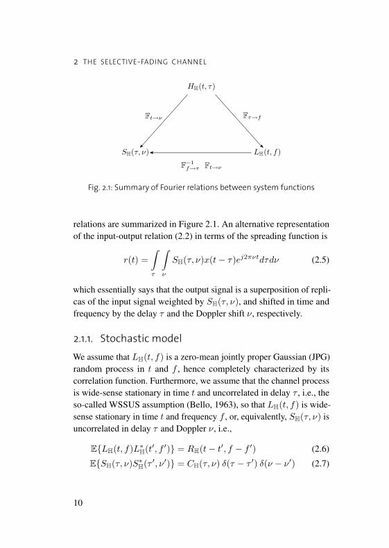
Fig. 2.1: Summary of Fourier relations between system functions
relations are summarized in Figure 2.1. An alternative representationof the input-output relation (2.2) in terms of the spreading function is
r(t) =∫τ
∫ν
SH(τ, ν)x(t− τ)ej2πνtdτdν (2.5)
which essentially says that the output signal is a superposition of repli-cas of the input signal weighted by SH(τ, ν), and shifted in time andfrequency by the delay τ and the Doppler shift ν, respectively.
2.1.1. Stochastic modelWe assume that LH(t, f) is a zero-mean jointly proper Gaussian (JPG)random process in t and f , hence completely characterized by itscorrelation function. Furthermore, we assume that the channel processis wide-sense stationary in time t and uncorrelated in delay τ , i.e., theso-called WSSUS assumption (Bello, 1963), so that LH(t, f) is wide-sense stationary in time t and frequency f , or, equivalently, SH(τ, ν) isuncorrelated in delay τ and Doppler ν, i.e.,
E{LH(t, f)L∗H(t′, f ′)} = RH(t− t′, f − f ′) (2.6)
E{SH(τ, ν)S∗H(τ ′, ν′)} = CH(τ, ν) δ(τ − τ ′) δ(ν − ν′) (2.7)
10
2.1 THE UNDERSPREAD FADING CHANNEL
where the scattering function CH(τ, ν) and the time-frequency corre-lation function RH(t, f) are related by the two-dimensional Fourierrelation
CH(τ, ν) =∫t
∫f
RH(t, f)e−j2π(νt−τf)dt df. (2.8)
Since RH(t, f) is stationary in both t and f , the scattering functionis nonnegative and real-valued for all τ and ν. It can therefore beinterpreted as the spectrum of the channel process.
2.1.2. The underspread assumptionBecause the transmitter, receiver, and the objects in the scatteringenvironment have finite velocities, the maximum Doppler shift ν0
experienced by the transmitted signal is finite. Similarly, we presumethat multipath propagation incurs a finite delay that is at most τ0. Forsimplicity, we assume, without loss of generality, that the scatteringfunction is compactly supported on the rectangle [0, τ0]× [0, ν0], i.e.,
CH(τ, ν) = 0 for (τ, ν) /∈ [0, τ0]× [0, ν0].
Note that the spreading function SH(τ, ν) is also supported in thisrectangle with probability 1 (w.p. 1). The channel spread is given by thequantity ∆H = ν0τ0. The underspread assumption, which implies thatthe total channel spread satisfies ∆H < 1 (Kozek, 1997), is relevantas most mobile radio channels are (highly) underspread. Moreover,underspread channels have a set of approximate eigenfunctions thatyield a discretized input-output relation as discussed next.
2.1.3. Approximate diagonalizationWe build our developments on the fact that underspread channelsare approximately diagonalized by orthogonal Weyl-Heisenberg bases
11

2 THE SELECTIVE-FADING CHANNEL
(Kozek, 1997) which are obtained by time-frequency shifting a proto-typing pulse g(t) as
gm,k(t) = g(t−mT )ej2πkFt
where
〈gm,k, gn,p〉 =∫t
gm,k(t)g∗n,p(t)dt = δm,nδk,p. (2.9)
In order to satisfy the orthogonality requirement on the basis {gm,k(t)},the grid parameters T and F are assumed to satisfy TF ≥ 1 (Kozek,1997; Kozek and Molisch, 1998). Note that large values of the productTF allow a better time-frequency localization of the prototyping pulseg(t), but result in a loss of signal space dimension in comparison to thecase TF = 1.
Since the spreading function SH(τ, ν) is strictly limited in delayτ and Doppler ν, by virtue of the Fourier relation between LH(t, f)and SH(τ, ν), the time-varying transfer function LH(t, f) is exactlycharacterized by its samples LH(mT, kF ) taken on a regular gridsatisfying the Nyquist conditions T ≤ 1
ν0and F ≤ 1
τ0. With this choice
of grid parameters, it has been shown (Kozek, 1997) that the kernelKH(t, t′) admits the following approximate eigenvalue decomposition
KH(t, t′) =∞∑
m=−∞
∞∑k=−∞
LH(mT, kF ) gm,k(t)g∗m,k(t′). (2.10)
The error associated with the approximate decomposition (2.10), whichis characterized for example in (Durisi et al., 2008), will be neglectedin our developments. We stress, however, that the choice of prototypingfunction g(t) is crucial in obtaining (2.10) : g(t) should depend on theshape of the scattering function CH(τ, ν) and be well localized in timeand frequency (Kozek, 1997; Kozek and Molisch, 1998; Matz et al.,2007; Durisi et al., 2008).
12

2.1 THE UNDERSPREAD FADING CHANNEL
2.1.4. Canonical signaling schemeThe above approximate diagonalization does not require channel infor-mation at the transmitter nor at the receiver. In particular, the transmitsignal can be constructed as a linear combination of the basis functions{gm,k(t)} as
x(t) =∞∑
m=−∞
K−1∑k=0
xm,k gm,k(t) (2.11)
where xm,k is the information bearing data symbol corresponding tothe time-frequency slot (m, k). Since the prototyping function g(t) iswell-localized in frequency by construction and practically realizablesignals are band limited, we have assumed that the input signal has aneffective bandwidth W = KF .
The receiver computes the inner products ym,k = 〈y, gm,k〉, wherey(t) = r(t) + z(t) and z(t) is additive white Gaussian noise withE{z(t)z∗(t′)} = δ(t − t′). Introducing the normalization xm,k =xm,k/
√SNR, with SNR denoting the average signal-to-noise ratio
(SNR), the overall input-output relation is hence given by
ym,k = 〈H x, gm,k〉+ 〈z, gm,k〉︸ ︷︷ ︸zm,k
=√
SNR∑n,p
xn,p 〈H gn,p, gm,k〉+ zm,k (2.12)
=√
SNR LH(mT, kF ) xm,k + zm,k (2.13)
where (2.12) is a direct consequence of the input signal structure in(2.11), and (2.13) follows from the approximate diagonalization (2.10)and the orthonormality of the set {gm,k(t)}. The projections of thenoise process onto the Weyl-Heisenberg basis are independent andidentically distributed across m and k, i.e., zm,k ∼ CN (0, 1), for allm and k, and E
{zm,kz
∗n,p
}= δm,nδk,p.
13

2 THE SELECTIVE-FADING CHANNEL
In essence, this scheme corresponds to transmitting and receivingon the channel’s approximate eigenfunctions and, hence, it yields anapproximate diagonalization of the channel. The canonical signalingscheme in (2.11) can be interpreted in terms of a pulse-shaped or-thogonal frequency-division multiplexing (OFDM) system, where thedata symbols xm,k are modulated onto a set of orthogonal signals(Durisi et al., 2008). According to this interpretation, the error result-ing in approximating KH(t, t′) as in (2.10) corresponds to intersymbolinterference (ISI) and intercarrier interference (ICI). Thus, (2.13) can bethought of as the input-output relation corresponding to a pulse-shapedOFDM system in which the ISI and ICI terms are neglected. Minimiz-ing the interference terms, and, hence, the error in the approximation(2.10), can by accomplished by appropriate design of the prototypingpulse g(t) and a proper choice of the grid parameters T and F (Kozekand Molisch, 1998; Durisi et al., 2008). Throughout this thesis, weshall assume that g(t), T , and F are chosen so that the approximationerror in (2.10) can be neglected.
2.2. SYSTEM MODEL
The system models employed throughout the thesis are based on theapproximate diagonalization of underspread WSSUS channels by Weyl-Heisenberg bases presented above. A precise description of the modelscorresponding to the point-point and MA cases is given at the beginningof Chapter 4 and Chapter 6, respectively. However, we shall nextexamine in further detail some aspects that are common to both casesdue to their common underlying structure.
Time-frequency slot mapping and input-output relations
We assume that communication takes place over M time slots and Kfrequency slots so that, for the sake of notation, we use the bijective
14

2.2 SYSTEM MODEL
mappingM, defined as
M : [0 : M − 1]× [0 : K − 1] −→ [0 : N − 1]
(m, k) 7−→ n = mK + k(2.14)
to index any time-frequency slot (m, k) in (2.13) by n = M(m, k).Moreover, we extend the input-output relation (2.13) to a MIMO chan-nel with MT transmit and MR receive antennas, assuming for simplicitythat the scalar subchannels of the MT ×MR MIMO channel have sta-tistically independent kernels with identical statistics, i.e., identicalscattering functions. Consequently, all subchannels are approximatelydiagonalized by the same Weyl-Heisenberg basis so that, based on(2.13) and the mapping in (2.14), we get
yn =√
SNR
MTHnxn + zn, n = 0, 1, . . . , N − 1 (2.15)
where SNR is the average signal-to-noise ratio at each receive antenna,yn, xn and zn denote, respectively, the corresponding MR × 1 receivesignal vector, MT × 1 transmit signal vector and MR × 1 JPG noisevector satisfying zn ∼ CN (0, IMR). The channel matrices are givenby Hn(i, j) = L
(i,j)H (mT, kF ) (i = 1, 2, . . . ,MR, j = 1, 2, . . . ,MT),
where the superscript (i, j) designates the time-varying transfer func-tion corresponding to the subchannel between transmit antenna j andreceive antenna i.
In the MA case, we shall assume that channels corresponding todifferent users are statistically independent with identical statistics.Hence, by the same line of reasoning as before, the correspondinginput-output relation follows as
yn =√
SNR
MT
U−1∑u=0
Hu,nxu,n + zn, n = 0, 1, . . . , N − 1 (2.16)
where xu,n is the transmit signal vector for user u ∈ U = {1, 2, . . . , U}and the corresponding channel matrix Hu,n has entries Hu,n(i, j) =LH
(i,j,u)(mT, kF ).
15

2 THE SELECTIVE-FADING CHANNEL
Statistics of the discrete fading process
Because the scalar subchannels are assumed to be JPG processes havingstatistically independent kernels with identical statistics, the channelmatrices are spatially uncorrelated and the correlation across slots isrelated to the time-frequency correlation function (2.6) as
E{Hn(i, j)(Hn′(i, j))∗} = RH((m−m′)T, (k − k′)F ),
i = 1, 2, . . . ,MR, j = 1, 2, . . . ,MT (2.17)
where n =M(m, k) and n′ =M(m′, k′), with n, n′ = 0, 1, . . . , N−1, are two time-frequency slots. In the MA case, we have
E{Hu,n(i, j)(Hu′,n′(i, j))∗} = RH((m−m′)T, (k−k′)F )δ(u−u′),i = 1, 2, . . . ,MR, j = 1, 2, . . . ,MT (2.18)
where u and u′ are two arbitrary users. For later reference, we definethe N ×N covariance matrix RH as
RH(n, n′) = RH((m−m′)T, (k − k′)F ). (2.19)
Clearly, RH follows from the time-frequency correlation functionRH(t, f), the mapping (2.14), and the relation (2.17). Hence, in gen-eral, RH is a two-level Toeplitz matrix, i.e., a Toeplitz-block-Toeplitzmatrix.
The two-dimensional power spectral density of the process is givenby
S(ξ, µ) =∞∑
m=−∞
∞∑k=−∞
RH(mT, kF ) e−j2π(mµ−kξ),
0 ≤ ξ, µ < 1. (2.20)
The power spectral density S(ξ, µ) can be related to the scattering
16

2.2 SYSTEM MODEL
function as follows
S(ξ, µ) =∞∑
m=−∞
∞∑k=−∞
e−j2π(mµ−kξ)×∫ν
∫τ
CH(τ, ν) ej2π(νmT−τkF )dτ dν (2.21)
=∫ν
∫τ
CH(τ, ν)∞∑
m=−∞ej2πmT (ν− µ
T )×
∞∑k=−∞
e−j2πkF (τ− ξF ) dτ dν
=1TF
∫ν
∫τ
CH(τ, ν)∞∑
m=−∞δ
(ν − µ−m
T
)×
∞∑k=−∞
δ
(τ − ξ − k
F
)dτ dν (2.22)
=1TF
∞∑m=−∞
∞∑k=−∞
CH
(ξ − kF
,µ−mT
)(2.23)
where we have used (2.8) to get (2.21), and (2.22) is a consequenceof Poisson’s sum formula. The variance of each channel coefficientsatisfies
σ2H =
∫τ
∫ν
CH(τ, ν) dτdν. (2.24)
We conclude this chapter with the following remarks. First, we em-phasize that the input-ouput relations in (2.15) and (2.16) presumethat the time-varying transfer functions are characterized by the samescattering function CH(τ, ν). An important implication of this assump-tion is that the channel’s correlation across time-frequency slots isdescribed by the same covariance matrix RH given in (2.19) for allspatial subchannels and all users.
17
2 THE SELECTIVE-FADING CHANNEL
Second, we note that the input-ouput relations obtained here encom-pass many simple channel models in addition to the WSSUS model(see the discussion on linear frequency-invariant (LFI) and linear time-invariant (LTI) channels in Appendix A). The results developed inthe sequel do therefore apply to these models provided one takes intoaccount the corresponding structural differences when pertinent. Weshall explicitly consider the most important instances of theses modelsin our exposition.
18

CHAPTER 3
The Diversity-Multiplexing Tradeoff
RATE AND RELIABILITY are two essential characteristics ofcommunication systems that have been widely studied by in-formation theorists. Shannon proved that channel capacity is
the maximum rate at which reliable communication is achievable: forany rate below capacity there exist encoders and decoders that achievearbitrarily small error probabilities and, conversely, error probability isbounded away from zero for any rate above capacity (Shannon, 1948).
Approaching error-free performance at rates below capacity requiresthe use of complex coding schemes with large block lengths. The theoryof error exponents developed by Gallager (1968) provides tools tocharacterize the maximum decay, or error exponent, of error probabilitywith block length. The error exponent is a decreasing function of therate, which is to say, rate and reliability are subject to a fundamentaltradeoff: an increase in rate comes at the expense of error performanceand vice versa. Unfortunately, a precise characterization of how rateand probability of error interplay is a difficult task in general.
The diversity-multiplexing (DM) tradeoff framework introduced byZheng and Tse (2003) has proved to be an efficient tool to elegantlycapture the rate-reliability tradeoff in fading channels. In contrast to theerror exponent approach, this new framework develops an asymptoticanalysis in signal-to-noise ratio (SNR) in lieu of block length.
19

3 THE DIVERSITY-MULTIPLEXING TRADEOFF
In this chapter, we review the fundamentals of the DM tradeoffframework as it constitutes the conceptual foundation for the resultspresented in this thesis. We start by discussing the framework forpoint-to-point flat-fading channels (Zheng and Tse, 2003), and we shallsubsequently address its extension to flat-fading multiple-access (MA)channels (Tse et al., 2004). Note that the concepts developed below willbe generalized to the selective-fading case in Chapter 4 and Chapter 6.
3.1. PRELIMINARIES
In flat-fading multiple-input multiple-output (MIMO) channels, theMR ×MT channel matrix H0 remains fixed so that the input-ouputrelation over a block of N slots is obtained from (2.15) as
Y =√
SNR
MTH0 X + Z (3.1)
where X = [x0 x1 · · · xN−1] denotes the MT × N input codewordand Y = [y0 y1 · · · yN−1] is the MR × N received matrix. TheMR × N additive noise matrix Z satisfies Z(i, j) ∼ CN (0, 1), ∀i, j.We are interested in the situation where the receiver has channel stateinformation (CSI), but the transmitter has only access to the fadinglaw. The DM tradeoff framework examines system performance forfixed block length when both the data rate and the error probabilityare allowed to scale with SNR. In this context, rate and reliability arerespectively captured by the somewhat coarser notions of multiplexingand diversity.
3.1.1. Rate and multiplexingAssuming a code that spans infinitely many independent realizations ofthe channel with input-output relation (3.1), the maximum rate that canbe reliably transmitted with CSI at the receiver is given by the ergodic
20

3.1 PRELIMINARIES
capacity (Telatar, 1999)
C(SNR) = E{
log det(
I +SNR
MTH0HH
0
)}. (3.2)
Asymptotically in SNR, it can be shown that (3.2) statisfies (Foschini,1996)
C(SNR) = min(MT,MR) log SNR + O(1) (3.3)
where the factor m , min(MT,MR), known as the (maximum) mul-tiplexing gain, represents the number of parallel data pipes that areavailable for data transmission in a given bandwidth and at a certaintransmit power. At high SNR, the multiplexing gain constitutes themaximal increase in data rate that can be obtained by increasing theSNR. For instance, by increasing SNR by 3 dB, m additional bits (persecond per Hertz) can be reliably conveyed through the channel.
3.1.2. Reliability and diversityThe drops in signal power that characterize fading channels result inhigh detection error probabilities. Diversity techniques can improve er-ror performance by providing the receiver with multiple independently-faded replicas of the same transmit signal. The probability of having allreplicas experiencing a deep fade simultaneously is then drastically re-duced. Indeed, assuming d i.i.d. Rayleigh fading branches, the averageerror probability can be shown to satisfy
P(error) = O(SNR−d
). (3.4)
Time and frequency diversity can be realized using standard forwarderror correcting codes in conjunction with interleaving (Proakis, 2001;Biglieri, 2005). Antenna diversity can be exploited at the receiver(Jakes, 1974) and/or at the transmitter, for example, by appropriatelycoding across transmit antennas (Alamouti, 1998; Tarokh et al., 1998,1999; Guey et al., 1999; Bölcskei and Paulraj, 2000), or by converting
21

3 THE DIVERSITY-MULTIPLEXING TRADEOFF
spatial diversity into time or frequency diversity and using then standardcoding techniques (Hiroike et al., 1992; Wittneben, 1993; Seshadri andWinters, 1994; Kuo and Fitz, 1997).
Two systems satisfying (3.4) may have drastically different errorperformance at fixed SNR, e.g., because they use codes with differentgains. Asymptotically in SNR, however, the error performance turnsout to be completely determined by the exponent d. Since we focus onthe high-SNR regime, we shall use the SNR exponent d as a measureof reliability.
3.1.3. System definitionsThe central concept invoked in the DM tradeoff framework to study theinterrelation between rate and reliability is that of family of codes. Afamily of codes Cr is a sequence of codebooks Cr(SNR) parametrizedby SNR. At a given SNR, the corresponding codebook Cr(SNR) con-tains SNRNr codewords, implying that the data rate scales with SNR asR(SNR) = r log SNR, where r is the multiplexing rate. More formally,we have the following definition.
Definition 3.1. A family of codes Cr operates at multiplexing rater ∈ [0,m] if the rate R(SNR) corresponding to the codebook Cr(SNR)satisfies
limSNR→∞
R(SNR)log SNR
= r. (3.5)
The multiplexing rate r is a fraction of the maximum multiplexinggain min(MT,MR) obtained in (3.3), which is to say that the family ofcodes Cr achieves a non-vanishing fraction of the ergodic capacity (3.2)as SNR increases. We also note that the multiplexing rate correspondingto a family of codes with fixed rate equals zero because, however largethe latter may be, the limit in (3.5) for such a family is zero.
The concept of family of codes enables us to characterize the rate-reliability tradeoff by relating the diversity achieved by Cr, i.e., thereliability associated to Cr which is measured by the SNR exponent
22

3.2 PERFORMANCE LIMITS
of the corresponding error probability, to its multiplexing rate r. Thisanalysis gives rise to the DM tradeoff, which is formally defined asfollows.
Definition 3.2. The DM tradeoff realized by Cr is given by the function
d(Cr) = − limSNR→∞
logPe(Cr)log SNR
(3.6)
where Pe(Cr) is the error probability obtained through maximum-likelihood (ML) detection. Moreover, the optimal DM tradeoff curve
d?(r) = supCr
d(Cr) (3.7)
quantifies the maximum achievable diversity gain over all families ofcodes that operate at multiplexing rate r.
In contrast to the traditional concept of diversity gain which is usedto characterize the high-SNR performance of a single codebook, theDM tradeoff d(Cr) is a performance measure associated with the en-tire family of codes Cr. Both the data rate and the error probabilitycorresponding to Cr scale with SNR, and the function d(Cr) capturestheir tradeoff in the high-SNR limit. As we shall see in the next section,there exists a fundamental limit to the optimal DM tradeoff d?(r) thatis dictated by the fading channel.
Throughout the rest of this thesis, two functions f(x) and g(x) aresaid to be exponentially equal, denoted by f(x) .= g(x), if and only if
limx→∞
log f(x)log x
= limx→∞
log g(x)log x
. (3.8)
Exponential inequality, denoted by ≤ and ≥, is defined analogously.
3.2. PERFORMANCE LIMITS
In the situation where coding is performed over a single realization ofthe fading channel with input-output relation (3.1), the ergodic capacity
23

3 THE DIVERSITY-MULTIPLEXING TRADEOFF
has no operational meaning. Indeed, there is a nonzero probabilityto encounter a channel realization that does not support the rate ofcommunication, however small it may be. In this case, we resort tothe outage capacity formulation (Ozarow et al., 1994; Telatar, 1999) todetermine the maximum rate at which reliable communication can besupported for some prescribed probability of outage. We shall see thatoutage capacity constitutes a fundamental performance limit not onlyfor large block lengths but also asymptotically in SNR.
3.2.1. Outage probabilityWe assume that the receiver has perfect CSI but the transmitter hasonly access to the fading law. An outage event occurs when the mutualinformation associated with the channel realization H0 is below thetarget data rate R, i.e.,
1NI(X; Y |H0) < R. (3.9)
The corresponding outage probability follows from optimizing themutual information over the input distribution f(X) as
Pout(R) = inff(X)
P(
1NI(X; Y|H0) < R
). (3.10)
The optimal distribution is Gaussian with vec(X) ∼ CN (0,Q). WhileTelatar (1999) conjectures that the optimal input covariance Q is diag-onal and the available power is evenly split over some or all transmitantennas depending on the SNR and R, no general proof is available.In the high-SNR regime, however, Zheng and Tse (2003) show thata covariance matrix satisfying Q = I incurs no loss of optimality;consequently, we can write
Pout(R) .= P(
log det(
I +SNR
MTH0HH
0
)< R
). (3.11)
24

3.2 PERFORMANCE LIMITS
The outage event can be related to the “level of singularity” of thechannel matrix. To this end, define the singularity levels (in descendingorder)
µk = − log λk(H0HH0 )
log SNR, k = 1, 2, . . . ,m, (3.12)
where the eigenvalues of the channel matrix λk(H0HH0 ) are arranged
in ascending order. With this notation, it has been shown in (Zhengand Tse, 2003, Th. 4) that the outage probability at rate R(SNR) =r log SNR satisfies the following exponential equality:
Pout(r log SNR) .= P(Or) (3.13)
where the outage event Or is given by
Or ={µ ∈ Rm
+ : µ1 ≥ µ2 ≥ . . . ≥ µm,
m∑k=1
[1−µk]+< r
}(3.14)
with µ = [µ1 µ2 . . . µm]. The definition (3.14) provides a parameteri-zation of the outage event Or in terms of the singularity levels of thechannel matrix. We shall see in the sequel that the outage probability(3.13) can be explicitly evaluated. First, we present a result that confersto P(Or) a central role in the analysis of the high-SNR performancelimits of communication.
3.2.2. Performance boundThe outage probability constitutes the ultimate performance in thehigh-SNR regime. Next, we state this fundamental result.
Theorem 3.1 (Zheng and Tse (2003)). For any family of codes Cr, theerror probability Pe(Cr) satisfies
Pe(Cr) ≥P(Or). (3.15)
25

3 THE DIVERSITY-MULTIPLEXING TRADEOFF
Proof. Fix a codebook Cr(SNR) with SNRNr codewords, and assumethat the transmit codeword X is uniformly drawn from Cr(SNR) inde-pendently of the channel realization H0. By Fano’s inequality (Coverand Thomas, 1991, Thm. 2.10.1), the probability of a detection errorEr (conditional on the channel realization) satisfies
1 + P(Er |H0) log |Cr(SNR)| ≥ H(X |Y,H0) (3.16)
where H(·) denotes the entropy function. Since X is independentof H0 and uniformly drawn from Cr(SNR), we have H(X |H0) =Nr log SNR and, hence, adding the mutual information IC(X; Y|H0)to both sides of (3.16) and performing some additional manipulationsyields
P(Er |H0) ≥ 1− IC(X; Y|H0)Nr log SNR
− 1Nr log SNR
. (3.17)
For ε > 0, define the set
Or(ε) = {H0 : IC(X; Y|H0) ≤ Nr(1− ε) log SNR}
and note that for any channel realization in Or(ε), it follows from(3.17) that
P(Er |H0 ∈ Or(ε)) ≥ ε− 1Nr log SNR
. (3.18)
Averaging the error probability over the channel distribution yields
Pe(Cr) = E{P(Er |H0)}
≥ E{
P(Er |H0)∣∣H0 ∈ Or(ε)
}(3.19)
≥(ε− 1
Nr log SNR
)P(Or(ε)) (3.20)
≥ P(Or(1−ε)) (3.21)
26

3.2 PERFORMANCE LIMITS
where (3.20) follows from using (3.18) in (3.19), and (3.21) is a con-sequence of taking the exponential limit in SNR and invoking theoptimality (in the sense of the outage probability) of i.i.d. Gaussiancodebooks in this regime. The claim follows by taking ε arbitrarilyclose to zero.
Since the outage probability P(Or) constitutes a lower bound to theerror probability of any family of codes, the best DM tradeoff curvemust satisfy
d?(r) ≤ dO(r) (3.22)
where the outage curve dO(r) is defined as
dO(r) , − limSNR→∞
log P(Or)log SNR
. (3.23)
It is well known that the outage probability is the ultimate perfor-mance for infinite block length: for a given channel realization, anyrate below mutual information can be conveyed with vanishing errorprobability as the block length tends to infinity. Theorem 3.1 says thatoutage probability is also the ultimate performance for finite blocklengths, bringing thus the question of whether there exist families ofcodes that can achieve that performance asymptotically in SNR (insteadof block length). In the case of flat-fading, Zheng and Tse (2003) haveshown the existence of such codes as we detail next.
3.2.3. AchievabilityThe outage bound of Theorem 3.1 is actually achievable in the flat-fading case. Next, we summarize this result by Zheng and Tse (2003).
Theorem 3.2 (Zheng and Tse (2003)). In the flat-fading channel, theoptimal DM tradeoff among all family of codes Cr with block lengthN ≥ MT + MR − 1 satisfies
d?(r) = dO(r), ∀r ∈ [0,m]. (3.24)
27

3 THE DIVERSITY-MULTIPLEXING TRADEOFF
This result says that there exist good families of codes Cr that achievethe outage bound. The error probability of such schemes is exponen-tially equal to the outage probability, which essentially means that thetypical way an error occurs is to encounter a channel realization that isin outage. While the existence of codes that approach the outage boundin the limit of infinite block length is well established, the fact that thisperformance bound is achievable asymptotically in SNR but with finiteblock lengths is remarkable.
The proof of Theorem 3.2 consists in averaging the error probabilityover the ensemble of Gaussian codes, and noting that for sufficientlylarge block lengths, i.e., larger than MT + MR − 1, the SNR exponentof the error probability is not larger than that of the outage probability.Although this result establishes the existence of optimal codes, it doesnot give any indication on how to construct them. Sparked by this result,a number of DM tradeoff optimal encoding and decoding schemes havebeen found during the past few years. In particular, the non-vanishingdeterminant criterion (Belfiore and Rekaya, 2003; Yao and Wornell,2003) on codeword difference matrices has been shown to constitute asufficient condition for DM tradeoff optimality in flat-fading MIMOchannels with two transmit and two or more receive antennas (Yaoand Wornell, 2003); this criterion has led to the construction of space-time codes based on constellation rotation (Yao and Wornell, 2003;Dayal and Varanasi, 2005) and cyclic division algebras (Belfiore et al.,2005). In (El Gamal et al., 2004), lattice-based space-time codes havebeen shown to be DM tradeoff optimal. The DM tradeoff optimality ofapproximately universal space-time codes was established in (Tavildarand Viswanath, 2006).
28

3.3 EVALUATION OF THE OUTAGE PROBABILITY
3.3. EVALUATION OF THE OUTAGEPROBABILITY
In flat fading, the distribution of the Hermitian matrix H0HH0 is known
as the Wishart distribution, and the joint density of its eigenvalues λk =λk(H0HH
0 ), k = 1, 2, . . . ,m, is given by (James, 1964; Muirhead,1982; Edelman, 1989)
fλ(λ1, λ2, . . . , λm) = K
m∏k=1
λM−mk
∏j<k
(λk−λj)2 exp
(−
m∑k=1
λk
),
(3.25)where 0 ≤ λ1 ≤ λ2 ≤ . . . ≤ λm, M , max(MT,MR) and K is anormalizing constant. Using (3.25), we shall see next how to evaluatethe outage probability (3.13).
The parameterization of the outage event (3.14) shows that someeigenvalues of H0HH
0 must decay with SNR for an outage to occur atmultiplexing rate r > 0, or, equivalently, some singularities µk’s mustbe positive, in which case the channel matrix is near singular. Motivatedby this observation, we approximate the joint eigenvalue distribution(3.25) in the vicinity of zero. First, using the standard approximationof the exponential function around zero, we write
e−λk = 1 + o(λk) . (3.26)
Then, the eigenvalue ordering yields λk − λj < λk for all j < k, andhence, we get∏
j<k
(λk − λj)2 =∏j<k
o(λ2k
)= o
(λ
2(k−1)k
). (3.27)
Inserting (3.26) and (3.27) into (3.25) yields
fλ(λ1, λ2, . . . , λm) = K
m∏k=1
(1 + o(λk)) o(λ2k−2+M−mk
)
29

3 THE DIVERSITY-MULTIPLEXING TRADEOFF
=m∏k=1
o(λ2k−2+M−mk
). (3.28)
From (3.12), the eigenvalues are related to the singularity levels accord-ing to λk = SNR−µk , k = 1, 2, . . . ,m. Using this variable change in(3.28) yields the following asymptotic expression for (3.25):
fµ(µ1, µ2, . . . , µm) .=m∏k=1
SNR−(2k−1+M−m)µk
= SNR−Pmk=1(2k−1+M−m)µk . (3.29)
We can now use this approximation of the distribution of µ aroundzero∗ to compute P(Or). First, the outage probability is trivially lowerbounded as
P(Or) =∫Or
fµ(µ1, µ2, . . . , µm) dµ
≥ supµ∈Or
fµ(µ1, µ2, . . . , µm). (3.30)
On the other hand, we have the natural upper bound
P(Or) ≤ ∫Or
dµ
supµ∈Or
fµ(µ1, µ2, . . . , µm). (3.31)
Note that the measure of Or is independent of SNR. Therefore, com-bining (3.30) and (3.31), and taking the limit in SNR yields
P(Or) .= supµ∈Or
fµ(µ1, µ2, . . . , µm)
.= SNR− infµ∈OrPmk=1(2k−1+M−m)µk (3.32)
∗Note that the substitution λk = εµk yields an expression similar to (3.29):fµ(µ1, µ2, . . . , µm) ≈ ε
Pmk=1(2k−1+M−m)µk for ε → 0. In our framework, we
set ε = SNR−1 to obtain a parameterization w.r.t. SNR.
30

3.3 EVALUATION OF THE OUTAGE PROBABILITY
where last step follows from (3.29). This simple reasoning suggeststhat the outage probability can be asymptotically approximated interms of the realization of µ in the set Or which is most likely to occur.Using large deviation techniques, both the approximation (3.29) and theasymptotic probability (3.32) have been rigorously derived by Zhengand Tse (2003). We summarize hereafter this result for later reference.
Theorem 3.3 (Zheng and Tse (2003)). For the flat-fading channel, theoutage probability satisfies
P(Or) .= SNR−dO(r) (3.33)
where
dO(r) = infµ∈Or
m∑k=1
(2k − 1 + M−m)µk. (3.34)
Moreover, the solution to (3.34) is given by the piecewise linear curveconnecting the points (r, dO(r)) for r = 0, 1, . . . ,m, and
dO(r) = (M− r)(m− r). (3.35)
There are many different realizations of the singularity vector µ inthe outage set Or, but Theorem 3.3 says that the outage probability isdominated (exponentially in SNR) by the probability corresponding tothe µ which minimizes the SNR exponent
∑mk=1(2k− 1 + M−m)µk.
We shall refer to the minimizing µ as the dominant outage event µ?.The solution (3.35) to the above optimization problem can be ob-
tained as follows. Assume that the multiplexing rate r is an integerwithin [0,m]. Then, µ? can be shown to satisfy (Zheng and Tse, 2003)
µ?k = 1, k = 1, 2, . . . ,m− r,µ?k = 0, k = m− r + 1,m− r + 2, . . . ,m,
(3.36)
which is to say that m− r eigenvalues decay with SNR as SNR−1 andr eigenvalues are constant w.r.t. SNR. Intuitively, the typical way an
31

3 THE DIVERSITY-MULTIPLEXING TRADEOFF
outage occurs at multiplexing rate r is to have r constant eigenvalueswhile the remaining ones decay to zero with SNR. The SNR exponentcorresponding to µ? is now given by
m−r∑k=1
(2k − 1 + M−m) = (M− r)(m− r)
which corresponds to (3.35). In the case of a non integer multiplexingrate, say r′ = r + δ with 0 < δ < 1, µ? can be shown to satisfyµ?m−r = 1 − δ and the remaining entries are still given by (3.36). Inother words, for an additional δ in multiplexing rate, the (m − r)theigenvalue of the channel corresponding to the dominant outage eventis adjusted by δ. Hence, the exponent dO(r) varies linearly betweeninteger values of multiplexing rate.
3.3.1. Geometric interpretationEquation (3.35) has a nice geometric interpretation in terms of the rankof the random channel matrix H0. Let w.l.o.g. m = MT and define theset
Mr ={H0 ∈ CM×m : rank(H0) = r
}.
Any matrix inMr has r independent columns with M entries and theremaining m− r columns are linear combinations thereof. Hence, sucha matrix can be specified by rM + r(m− r) = Mm− (M− r)(m− r)parameters, which can be thought of as the dimensionality∗ ofMr. Putdifferently, the matrix H0 will be close toMr when the components ofH0 lying in the (M−r)(m−r) dimensions orthogonal toMr are closeto zero. Since (M− r)(m− r) = dO(r) and the entries of H0 are i.i.d.CN (0, 1), the probability of having dO(r) entries in H0 of magnitudeSNR−1 (i.e., close to zero for large SNR) is given by SNR−dO(r). Thus,the outage probability SNR−dO(r) can be interpreted as the probabilitythat the random channel matrix is close toMr.∗Mr has a well-defined dimensionality. See Tse and Viswanath (2005) for more
details.
32

3.3 EVALUATION OF THE OUTAGE PROBABILITY
MmdO
(r) (M! 1)(m! 1)
(M! k)(m! k)
M!m + 1
0 1 k m! 1 m
r
Fig. 3.1: Outage curve dO(r) corresponding to a flat-fading MIMO channelwith m = min(MT,MR) and M = max(MT,MR).
3.3.2. Visualization of the tradeoffFigure 3.1 illustrates the optimal DM tradeoff dO(r). The best errorperformance is obtained for multiplexing rate r = 0, i.e., dO(0) =Mm, which basically says that maximum diversity gain can only to beachieved at fixed rates. On the other hand, at maximum multiplexingrate m, the system operates close to the ergodic capacity (3.2), and theoptimal diversity is given by dO(m) = 0, implying that an increasein SNR does not improve error performance. Between these extremepoints, the outage curve dO(r) is a strictly decreasing function of themultiplexing rate r: an increase in data rate comes at the expense ofdiversity and vice versa.
The relation between outage probability, rate, and SNR is illustrated
33
3 THE DIVERSITY-MULTIPLEXING TRADEOFF
0 5 10 15 20 25 30 35 40 45 5010-16
10-14
10-12
10-10
10-8
10-6
10-4
10-2
100
SNR in [dB]
Out
age
prob
abilit
y
dO(1) = 9 dO(2) = 4
dO(3) = 1
dO(0) = 16r = 0 r = 1 r = 2
r = 3
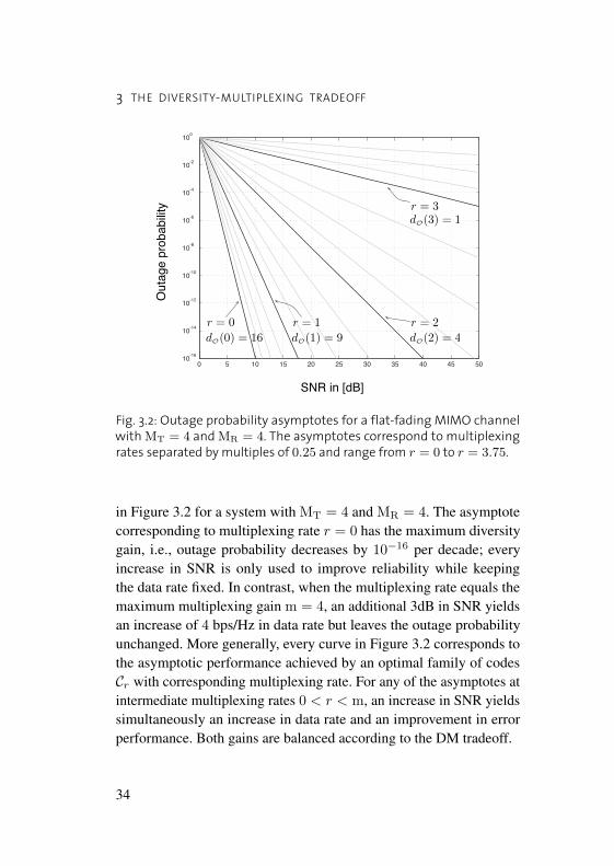
Fig. 3.2: Outage probability asymptotes for a flat-fading MIMO channelwith MT = 4 and MR = 4. The asymptotes correspond to multiplexingrates separated by multiples of 0.25 and range from r = 0 to r = 3.75.
in Figure 3.2 for a system with MT = 4 and MR = 4. The asymptotecorresponding to multiplexing rate r = 0 has the maximum diversitygain, i.e., outage probability decreases by 10−16 per decade; everyincrease in SNR is only used to improve reliability while keepingthe data rate fixed. In contrast, when the multiplexing rate equals themaximum multiplexing gain m = 4, an additional 3dB in SNR yieldsan increase of 4 bps/Hz in data rate but leaves the outage probabilityunchanged. More generally, every curve in Figure 3.2 corresponds tothe asymptotic performance achieved by an optimal family of codesCr with corresponding multiplexing rate. For any of the asymptotes atintermediate multiplexing rates 0 < r < m, an increase in SNR yieldssimultaneously an increase in data rate and an improvement in errorperformance. Both gains are balanced according to the DM tradeoff.
34
3.4 MULTIPLE-ACCESS CHANNEL
3.4 . MULTIPLE-ACCESS CHANNEL
The DM tradeoff framework can be extended to analyze fundamentalperformance limits of communication over MA channels (Tse et al.,2004). In this section, we prepare the ground for our study of MAselective-fading channels in Chapter 6 by reviewing prior work.
We start by extending the input-output relation (3.1) to MA channelsas follows:
Y =√
SNR
MT
U∑u=1
Hu,0 Xu + Z (3.37)
where the output matrix Y and the noise matrix Z are defined analo-gously to those in (3.1), but now the input consists of U codewordsXu = [xu,0 xu,1 · · · xu,N−1], one for each user. For the sake ofnotation, we set
HS,0 = [Hu1,0 Hu2,0 · · · Hu|S|,0]
XS = [XTu1
XTu2· · · XT
u|S| ]T
for any S = {u1, u2, . . . , u|S|} with S ⊆ U = {1, 2, . . . , U}. As inthe point-to-point case, we focus on the case where the receiver hasperfect CSI for all users, but the transmitters have only access to thefading law.
3.4.1. Achievable rate regions
In contrast to the point-to-point case where the maximum rate of re-liable communication is determined by a single quantity, any ratetuple (R1, R2, . . . , RU ) that is achievable, i.e., for which there existsequences of codes, one for each user, with vanishing error probabilitiesas block length increases, belongs to the so-called capacity region.
35

3 THE DIVERSITY-MULTIPLEXING TRADEOFF
Capacity region
The first characterizations of the capacity region were reported for theMA additive white Gaussian noise (AWGN) channel in the early 1970’s(Ahlswede, 1971; Liao, 1972; Wyner, 1974). Assuming momentarilythat the channel matrix HU,0 is deterministic, the capacity regioncorresponding to the MA channel in (3.37) is given by the followingtheorem.
Theorem 3.4 (Cover and Thomas (1991)). The capacity region of theU -user MA channel is the closure of the convex hull of the rate tuples(R1, R2, . . . , RU ) satisfying
R(S) =∑u∈S
Ru ≤ 1NI(XS ; Y |XS), ∀S ⊆ U (3.38)
for some product distribution f1(X1) · f2(X2) · · · · · fU (XU ).
Equation (3.38) gives rise to 2U − 1 constraints, one for every subsetof U , and maximizing the corresponding mutual information over theinput product distribution yields the boundaries of the capacity region.For a given set of users S ⊆ U , the largest boundary on R(S) is ob-tained with Gaussian codebooks. In particular, let xu,n be i.i.d. acrossslots n and independent across users u ∈ S with xu,n ∼ CN (0,Qu),where Qu is subject to the constraint Tr (Qu) ≤ MT. Then, the opti-mization problem reduces to
maxfu(Xu),u∈S
1NI(XS ; Y |XS) =
maxQu�0,u∈S
Tr(Qu)≤MT
log det
(I +
SNR
MT
∑u∈S
Hu,0QuHHu,0
). (3.39)
We note, however, that choosing {Qu} so as to maximize the mutualinformation corresponding to the set S does not necessarily maximizethe boundaries corresponding to the remaining sets of users. In general,
36

3.4 MULTIPLE-ACCESS CHANNEL
A
B
1N
I(X2;Y|X1)
1N
I(X1;Y|X2)
1N
I(X1,X2;Y)
R1
R2
R1 + R2 =
Fig. 3.3: Two achievable rate regions for the 2-user MA channel corre-sponding to different input distributions. Any rate tuple on the segmentAB can be achieved by time-sharing.
there is no unique input distribution that optimizes all boundaries. Thecapacity region in Theorem 3.4 is therefore given by the convex hullof all the achievable rate regions obtained from admissible (w.r.t. anindividual power constraint) input distributions. Taking the convex hullof all such regions is natural since convex combinations of rate tuplescan be achieved by time-sharing. Figure 3.3 illustrates two possiblerate regions for the 2-user MA channel arising from different inputdistributions. Rate tuples on the segment between the corner pointsA and B are achievable by time-sharing. In particular, if (R1, R2)is the rate tuple at A and (R′1, R
′2) is that at B, then any rate tuple
(λR1 + (1− λ)R′1, λR2 + (1− λ)R′2) for λ ∈ [0, 1] is achievable byoperating λ percent of the time at A and the rest at B.
37

3 THE DIVERSITY-MULTIPLEXING TRADEOFF
Ergodic capacity region
When coding is performed across infinitely many realizations of thechannel with input-ouput relation (3.37), the set of achievable ratestuples (R1, R2, . . . , RU ) is given by the ergodic capacity region withboundaries
R(S) ≤ maxQu�0,u∈S
Tr(Qu)≤MT
E
{log det
(I +
SNR
MT
∑u∈S
Hu,0QuHHu,0
)}(3.40)
for S ⊆ U . The solution can be found by recalling the point-to-pointcase treated in Section 3.1.1 for which the optimal input covarianceis given by Q = I. Put differently, the optimal strategy is to transmitindependent signals across antennas. With such signal structure, the factthat the users cannot cooperate in the MA case becomes immaterial, andwe can hence conclude that picking Qu = I for every u ∈ U is optimal(Telatar, 1999; Tse and Viswanath, 2005). Noteworthily, a unique inputproduct distribution simultaneously maximizes all constraints. Uponinserting the optimal covariance matrices into (3.40), we obtain thefollowing characterization of the ergodic capacity region in the high-SNR regime (Foschini, 1996)
R(S) ≤ min(MR, |S|MT) log SNR + O(1) , S ⊆ U . (3.41)
3.4.2. Multiple-access system definitionsParalleling Section 3.1.3, we invoke also in the MA case the conceptof family of codes whereby user u employs a sequence of codebooksCru(SNR), one for each SNR. The corresponding data rate scales withSNR as Ru(SNR) = ru log SNR, where ru ∈ [0,m] is the multiplex-ing rate. The family of codes Cru is assumed to have block length N sothat, at any given SNR, Cru(SNR) contains SNRNru codewords Xu.
38

3.4 MULTIPLE-ACCESS CHANNEL
Since there are multiple users, the overall family of codes is given by
Cr = Cr1 × Cr2 × · · · × CrUwhere r = (r1, r2, . . . , rU ) denotes the multiplexing rate tuple. At agiven SNR, the corresponding codebook Cr(SNR) contains SNRNr(U)
codewords with r(U) =∑Uu=1 ru. Invoking the high-SNR character-
ization of the ergodic capacity boundaries in (3.41), the sum of themultiplexing rates corresponding to the users in S ⊆ U satisfies
r(S) ,∑u∈S
ru ≤ min(MR, |S|MT).
The DM tradeoff realized by Cr is characterized by the function
d(Cr) = − limSNR→∞
logPe(Cr)log SNR
(3.42)
where Pe(Cr) is the total error probability (that is, the probability forthe receiver to make a detection error for at least one user) obtainedthrough ML detection. The optimal DM tradeoff curve
d?(r) = supCr
d(Cr) (3.43)
where the supremum is taken over all possible families of codes Cr,quantifies the maximum achievable diversity gain as a function of themultiplexing rate tuple r.
3.4.3. Outage formulationSince we are interested in characterizing ultimate performance limitsover a single realization of the channel with input-output relation (3.37),we shall use the concept of outage capacity (Ozarow et al., 1994; Telatar,1999; Tse et al., 2004) as we did previously in the point-to-point case.
Conditional on a realization of the fading channel matrix HU,0, theset of rates that are achievable over the channel (3.37) for perfect CSI
39

3 THE DIVERSITY-MULTIPLEXING TRADEOFF
at the receiver only are characterized by Theorem 3.4. As in the point-to-point case, it can be shown that one can restrict the input to be i.i.d.Gaussian without loss of optimality (Tse et al., 2004). Hence, the setof achievable rate tuples conditional on the channel realization HU,0satisfies the boundary constraints
R(S) ≤ log det
(I +
SNR
MT
∑u∈S
Hu,0HHu,0
), ∀S ⊆ U . (3.44)
If a given rate tuple (R1, R2, . . . , RU ) lies outside the region definedby (3.44), we say that the channel is in outage w.r.t. this rate tuple anddenote the corresponding outage probability by Pout(R1, R2, . . . , RU ).Letting the users’ rates scale with SNR as Ru(SNR) = ru log SNR, forall u, the outage probability satisfies
Pout(r1 log SNR, r2 log SNR, . . . , rU log SNR) .= P(Or) (3.45)
where Or shall be referred to as the outage event corresponding to themultiplexing rate tuple r. Before characterizing Or more precisely, wenote that, as in the point-to-point case, the outage probability constitutesa fundamental performance bound on any family of codes.
Theorem 3.5 (Tse et al. (2004)). Assuming an ML receiver, the detec-tion error probability of any family of codes Cr satisfies
d?(r) ≤ − limSNR→∞
log P(Or)log SNR
(3.46)
This result suggests that, irrespectively of the family of codes Cremployed for communication, detection errors are very likely to occurwhenever the channel is in outage with respect to the multiplexing ratetuple r.
Exploiting the structure of the rate region in (3.44), the outage prob-ability is naturally decomposed as follows
P(Or) = P
⋃S ⊆ U
OS (3.47)
40

3.4 MULTIPLE-ACCESS CHANNEL
where the S-outage event OS can be rigorously defined in terms of thesingularity levels of the channel matrices {Hu,0} just like the outageevent corresponding to the point-to-point case was defined in (3.14).For our purposes, it is sufficient to note that the S-outage probabilitysatisfies
P(OS) .= P
(log det
(I +
SNR
MT
∑u∈S
Hu,0HHu,0
)< R(S)
)(3.48)
.= SNR−dS(r(S)) (3.49)
where last step follows upon observing that (3.48) is equivalent to theoutage probability of a point-to-point flat-fading channel with |S|MT
transmit and MR receive antennas and, hence, invoking Theorem 3.3,the corresponding tradeoff curve is the piecewise linear function deter-mined by
dS(r) = (MR − r)(|S|MT − r),r = 0, 1, . . . ,min(MR, |S|MT). (3.50)
We conclude our review of the DM tradeoff in flat-fading MA channelswith the following result which characterizes the multiplexing rateregion, denoted byR(d), where all the users are guaranteed a certainlevel of diversity d.
Theorem 3.6 (Tse et al. (2004)). If the block length satisfies N ≥|S|MT + MR − 1, then there exist families of codes Cr for which themultiplexing rate region is given by
R(d) ={r : r(S) ≤ rS(d),∀S ⊆ U
}(3.51)
where rS(d) denotes the inverse of the function dS(r).
Theorem 3.6 says that the outage bound (3.46) is achievable. Theproof technique, analogous to that employed in the point-to-point case,
41

3 THE DIVERSITY-MULTIPLEXING TRADEOFF
establishes the existence of optimal codes in the Gaussian ensembleof codes. Recent work (Nam and El Gamal, 2007; Badr and Belfiore,2008b) provides explicit code constructions that achieve the optimaltradeoff.
3.5 . BEYOND FLAT FADING
The framework presented in this chapter allows to efficiently character-ize the tradeoff between rate and reliability in MIMO fading channels,and the outage bound, both in the point-to-point and multiple-accesscases, constitutes the ultimate performance limit for systems with fixedblock lengths. However, the proof techniques used in (Zheng and Tse,2003) to evaluate the outage probability and to establish the existenceof optimal codes are not directly applicable to the more general classof selective-fading channels. More precisely, characterizing dO(r) forthe selective-fading case seems analytically intractable with the maindifficulty stemming from the fact that one has to deal with the sum ofcorrelated terms in the expression for the mutual information. It turnsout, however, that one can find lower and upper bounds on I(SNR)which are exponentially tight (and, hence, preserve the DM tradeoffbehavior) and analytically tractable. In the next chapter, we present atechnique that formalizes this idea. We note that the ideas at the heart ofour technique have also proved to be useful in examining performancelimits for the relay channel (Akçaba et al., 2007).
42

CHAPTER 4
Performance Limits inSelective-Fading Channels
THE DIVERSITY-MULTIPLEXING (DM) tradeoff framework pre-sented in Chapter 3 allows to efficiently characterize the rate-reliability tradeoff over multiple-input multiple-output (MIMO)
flat-fading channels. The essence of the approach is to study the in-terrelation between the data rate and the error probability of a familyof codes parametrized by SNR. As the SNR increases, a precise char-acterization of the tradeoff emerges. The outage probability, whichconstitutes the ultimate limit on the performance of a family of codes,depends on the distribution of the fading channel. For this reason, theresults on the DM tradeoff summarized in Chapter 3 do only hold inthe flat-fading case.
In environments that are subject to temporal variations and/or mul-tipath propagation, the flat-fading channel model fails to capture thechannel’s inherent memory in frequency and time. In this case, thewireless channel is more accurately described in terms of the selective-fading channel model presented in Chapter 2. Since real world wirelesscommunication systems operate over channels that are selective both infrequency and in time, identifying the corresponding performance lim-its is pertinent. However, a characterization of the optimal DM tradeoff
43

4 PERFORMANCE LIMITS IN SELECTIVE-FADING CHANNELS
of this class of channels along with a code design criterion capable ofguaranteeing optimal performance remain to be found.
In this chapter, we present a technique that solves this problem byproviding exponentially tight upper and lower bounds on the outageprobability of coherent selective-fading MIMO channels. The idea un-derlying our approach is to analyze the “Jensen channel” associatedwith a given selective-fading MIMO channel. While the original prob-lem seems analytically intractable due to the mutual information beinga sum of correlated random variables, the Jensen channel is equivalentto the original channel in the sense of the DM tradeoff and lends itselfnicely to analytical treatment. In addition, our technique provides anexplicit code design criterion to guarantee DM tradeoff optimality inselective-fading MIMO channels. Our criterion ties in perfectly wellwith other criteria reported in prior work.
The rest of this chapter is organized as follows. Building on theselective-fading channel model examined in Chapter 2, we first in-troduce the system model that we shall adopt throughout the chapter.Section 4.2 presents a rigorous formulation of the problem at hand interms of the DM tradeoff framework. In Section 4.3, we introduce the“Jensen channel”, which is the principal tool employed to derive theoptimal tradeoff, and other related concepts such as the Jensen outageevent and the corresponding probability. We will then be able to derivethe optimal DM tradeoff in Section 4.4 by providing a code designcriterion that guarantees the error probability to be exponentially tightto the Jensen outage probability. Section 4.5 concludes this chapter bydiscussing the relation of our code design criterion with prior work.
4 .1. SIGNAL AND CHANNEL MODEL
The system model presented below is based on the considerations madein Chapter 2. We consider a point-to-point channel with MT transmitand MR receive antennas. The corresponding input-ouput relation is
44

4.1 SIGNAL AND CHANNEL MODEL
given by
yn =√
SNR
MTHnxn + zn, n = 0, 1, . . . , N − 1 (4.1)
where the index n = M(m, k) denotes a time, frequency, or time-frequency slot according to the mapping defined in (2.14), and SNR de-notes the average signal-to-noise ratio at each receive antenna. The vec-tors yn, xn, and zn denote, respectively, the MR×1 receive signal vec-tor, the MT×1 transmit signal vector, and the MR×1 zero-mean jointlyproper Gaussian (JPG) noise vector satisfying E
{znzHn′
}= δn,n′ I.
We also define the matrix Y = [y0 y1 · · · yN−1], and assume thatat any SNR level the codebook Cr(SNR) contains SNRNr codewordsX = [x0 x1 · · · xN−1] that satisfy the power constraint
‖X‖2F ≤ NMT,∀X ∈ Cr(SNR). (4.2)
This constraint implies that the codewords of any (with respect to (w.r.t.)SNR) codebook Cr(SNR) lie inside a sphere of radius
√NMT in
CMT×N centered at the origin. Because the sphere radius is constantw.r.t. SNR so are the entries of Cr(SNR). Yet the codeword differencematrix E = X−X′, where X,X′ ∈ Cr(SNR), does in general dependon SNR because the number of codewords packed within the sphereincreases as |Cr(SNR)| = SNRNr for the rate R(SNR) = r log SNR
to be sustained.In the case N = 1 and MT = 1, for example, an admissible Cr
would be a family of quadrature amplitude modulation (QAM) con-stellations with |Cr(SNR)| = SNRr points satisfying the constraintx2 ≤ 1. Note that the minimum distance in such a family of codesscales as∗ d2
min.= SNR−r, i.e., the area of the unit disk divided by the
number of constellation points in Cr(SNR).
∗A discussion of the DM tradeoff properties of QAM constellations for the scalarRayleigh fading channel can be found in (Tse and Viswanath, 2005, Section 9.1.2)
45

4 PERFORMANCE LIMITS IN SELECTIVE-FADING CHANNELS
We assume that the channel is spatially uncorrelated, but correlatedacross slots. Specifically, we let
E{Hn(i, j)(Hn′(i′, j′))∗} = RH(n, n′) δi,i′ δj,j′ ,
i, i′ = 1, 2, . . . ,MR, j, j′ = 1, 2, . . . ,MT
n, n′ = 0, 1, . . . , N − 1. (4.3)
The covariance matrix RH, for which we define ρ , rank(RH), fol-lows from the time-frequency correlation function in (2.17). Finally,we stack the channel matrices across slots according to
H = [H0 H1 · · · HN−1]. (4.4)
With this notation, we have
E{
vec(H)(vec(H))H}
= RH ⊗ IMTMR . (4.5)
We note that the input-output relation (4.1) can also be used to de-scribe communication over linear time-invariant and linear frequency-invariant channels. We refer the reader to Appendix A for a justificationof this statement. Unless explicitly indicated otherwise, we shall as-sume that the fading channel underlying (4.1) belongs to the class ofchannels which are approximately diagonalized by a suitably chosenWeyl-Heisenberg basis as explained in Chapter 2.
4 .2. PROBLEM FORMULATION
We consider the situation where the receiver has perfect channel stateinformation (CSI) while the transmitter does not have CSI but knowsthe channel law. Given a target outage probability, the transmitter candetermine the maximum rate that is supported by the channel andoptimize the family of codes Cr accordingly. In the high-SNR regime,the relation between outage probability and data rate for selective-fading MIMO channels is obtained as follows.
46

4.2 PROBLEM FORMULATION
Optimal input distribution
We assume without loss of optimality a Gaussian input distribution sothat the input codeword X satisfies vec(X) ∼ CN (0,Q) with average∗
power constraint Tr (Q) ≤ NMT. Then, the outage probability followsby optimizing over the input covariance as
Pout(R) = infQ�0
Tr(Q)≤NMT
P(
1N
log det(
I +SNR
MTDHQ DH
H
)< R
)(4.6)
where DH = diag{Hn}N−1n=0 . The optimal covariance matrix can be
explicitly obtained using the following arguments.First, any Q that is admissible under the power constraint yields
a lower bound to the maximum mutual information. In particular, bypicking Q = I, we get the following upper bound to the outage proba-bility:
Pout(R) ≤ P
(1N
N−1∑n=0
log det(
I +SNR
MTHnHH
n
)< R
). (4.7)
On the other hand, due to the power constraint, Q must satisfy thepositive semidefinite ordering Q � NMTI. Since the function f(A) =log det(I + A) is increasing over the cone of positive semidefinitematrices (S. Boyd and L. Vandenberghe, 2004), we obtain the lowerbound
Pout(R) ≥ P
(1N
N−1∑n=0
log det(I + SNRN HnHH
n
)< R
). (4.8)
The bounds in (4.7) and (4.8) are equal up to a factor that is independent
∗This average power constraint, which is a relaxation of the per-codeword constraint(4.2), serves only the purpose of establishing a bound on performance. It will laterbecome manifest that the bound we obtain is still achievable if we restrict our attentionto the subset of codes satisfying (4.2).
47

4 PERFORMANCE LIMITS IN SELECTIVE-FADING CHANNELS
of SNR and, therefore, in the high SNR limit we have
limSNR→∞
log P(
1N
∑N−1n=0 log det
(I + SNR
MTHnHH
n
)< R
)log SNR
= limSNR→∞
logPout(R)log SNR
= limSNR→∞
log P(
1N
∑N−1n=0 log det
(I + SNRN HnHH
n
)< R
)log SNR
.
We can thus conclude that an i.i.d. (across space and slots) Gaussianinput distribution achieves the optimal outage performance in the scaleof interest and, consequently, the outage probability satisfies the expo-nential equality
Pout(R) .= P(I(SNR) < R) (4.9)
where
I(SNR) =1N
N−1∑n=0
log det(
I +SNR
MTHnHH
n
). (4.10)
Maximum multiplexing rate
The multiplexing rate r is at most m = min(MT,MR) as the followingargument shows. By the same line of reasoning as in flat fading (Telatar,1999), we know that for selective fading a uniform input power allo-cation is optimal in the sense of the ergodic capacity (Bölcskei et al.,2002a; Tse and Viswanath, 2005). We therefore have
C(SNR) = E
{1N
N−1∑n=0
log det(
I +SNR
MTHnHH
n
)}
= E{
log det(
I +SNR
MTHmHH
m
)}(4.11)
48

4.2 PROBLEM FORMULATION
where m can be taken to be any slot as the fading process is stationary.It follows from our discussion in Section 3.1.1 that (4.11) satisfies
C(SNR) = m log SNR + O(1)
which, recalling Definition 3.1, means that the multiplexing rate rcannot exceed m. In general, the multiplexing rate satisfies r ∈ [0,m].
Outage event
As in the point-to-point case, the outage event can be characterizedin terms of the “level of singularity” of the channel matrices. To thisend, let the eigenvalues of the channel matrix corresponding to slot n(n = 0, 1, . . . , N − 1) be given in increasing order by
λk(HnHHn ), k = 1, 2, . . . ,m (4.12)
and define the singularity levels (in descending order across index k)
µk(n) = − log λk(HnHHn )
log SNR, k = 1, 2, . . . ,m. (4.13)
The mutual information in (4.10) can now be written as
I(SNR) =1N
N−1∑n=0
m∑k=1
log(
1 +SNR
MTλk(HnHH
n ))
=1N
N−1∑n=0
log
(m∏k=1
(1 +
SNR
MTSNR−µk(n)
))(4.14)
where last equality follows from the variable change (4.13). At highSNR, we have(
1 +SNR
MTSNR−µk(n)
).= SNR[1−µk(n)]+
49

4 PERFORMANCE LIMITS IN SELECTIVE-FADING CHANNELS
which, upon inserting into (4.14), yields
I(SNR) =
(1N
N−1∑n=0
m∑k=1
[1− µk(n)]+)
log SNR + O(1) . (4.15)
The dependence of the outage probability (4.9) on the singularity levelscan now be made explicit. Using (4.15) in (4.9) and letting the data ratescale with SNR as R(SNR) = r log SNR, we get
Pout(r log SNR) .= P(Or) (4.16)
where the outage event∗ Or is given by
Or ={µ(n) ∈ Rm
+ , n = 0, 1, . . . , N − 1 :
1N
N−1∑n=0
m∑k=1
[1− µk(n)]+< r
}. (4.17)
with µ(n) , [µ1(n) µ2(n) . . . µm(n)]. The outage probability (4.16)constitutes a lower bound to the error probability of any family ofcodes† Cr, which is to say that the optimal DM tradeoff satisfies
d?(r) ≤ dO(r) (4.18)
where we recall that
dO(r) = − limSNR→∞
log P(Or)log SNR
. (4.19)
The outage event (4.17) depends upon the singularity levels correspond-ing to the individual channel matrices. In order to directly compute the∗We note that (4.17) is a generalization of (3.14) to the case of selective-fading
channels, and it can be proved using the same arguments as in the proof of (3.14) givenby (Zheng and Tse, 2003).†The proof for this statement is omitted as it proceeds along the lines of the proof of
Theorem 3.1.
50

4.3 ANALYSIS TOOL
outage probability, one would need to know the joint distribution of thesingularity levels. Unfortunately, the latter is in general unknown forselective-fading channels. In the next sections, we develop a techniquethat bypasses this difficulty.
4 .3. ANALYSIS TOOL
Jensen’s inequality (Jensen, 1906), perhaps one of the most widelyused inequalities in mathematics and information theory, states that ifthe real function ϕ(x) is continuous and convex on some interval, then
ϕ
(∑n anxn∑n an
)≤∑n anϕ(xn)∑
n an(4.20)
where the real numbers {xn} do all belong to the interval, and the {an}are arbitrary positive numbers. This simple inequality underlies theforthcoming analysis of the DM tradeoff in selective-fading MIMOchannels as it gives rise to the concept of “Jensen channel”.
4.3.1. The Jensen channelConsider the mutual information in (4.10) and note that the matrix-valued arguments of the function log det(·) are positive definite. Wecan hence invoke the concavity of the function log det(·) over theconvex cone of positive definite matrices (e.g. Horn and Johnson, 1993,7.6.7) to get the following variant of Jensen’s inequality
I(SNR) ≤ log det
(I +
SNR
MTN
N−1∑n=0
HnHHn
). (4.21)
The upper bound to I(SNR) can be interpreted as the mutual informa-tion of an abstract channel that is associated with the original channel.This interpretation motivates the following definition.
51

4 PERFORMANCE LIMITS IN SELECTIVE-FADING CHANNELS
Definition 4.1. The Jensen channel is the m×NM matrix given by
H =
{[H0 H1 · · · HN−1], if MR ≤ MT,
[HH0 HH
1 · · · HHN−1], if MR > MT.
(4.22)
A general upper bound to the mutual information can now be writtenin terms of the Jensen channel H as
I(SNR) ≤ J(SNR) = log det(
I +SNR
MTNHHH
). (4.23)
The operational significance of the Jensen channel will be establishedin Section 4.4. We shall first introduce and characterize analytically theoutage probability corresponding to this channel.
4.3.2. The Jensen outage probabilityIn the following, we say that a Jensen outage occurs if the Jensenchannel H is in outage w.r.t. the target data rate R, i.e., H belongs tothe set {H : J(SNR) < R}. In analogy to the outage probability, wedefine the Jensen outage probability as
PJ(R) , P(J(SNR) < R) . (4.24)
Since J(SNR) is an upper bound to the mutual information, the set ofchannel realizations in Jensen outage is a subset of the realizations thatare in outage. This observation, illustrated in Figure 4.1, yields trivially
PJ(R) ≤ Pout(R). (4.25)
In the sequel, we will show that both probabilities are in fact expo-nentially equal, and hence the Jensen outage probability constitutes afundamental performance limit in the high-SNR regime. Before estab-lishing this somewhat surprising result, we shall develop an analyticalcharacterization of the Jensen outage probability.
52

4.3 ANALYSIS TOOL
{H0,H1, . . . ,HN!1}!H : I(SNR) < R
"
!H : J(SNR) < R"
Fig. 4.1: The set of channel matrices H0,H1, . . . ,HN−1 in Jensen outageis a subset of the channel matrices in outage.
High-SNR characterization
Using (4.5), we show in Appendix B that the Jensen channel satisfies
H = Hw(RT/2 ⊗ IM) (4.26)
where R = RH, if MR ≤ MT, and R = RTH , if MR > MT. The
matrix Hw is the i.i.d. CN (0, 1) matrix with the same dimensions asH given by
Hw =
{[Hw,0 Hw,1 . . . Hw,N−1], if MR ≤ MT,
[HHw,0 HH
w,1 . . . HHw,N−1], if MR > MT.
(4.27)
Here, the Hw,n denote i.i.d. CN (0, 1) matrices of dimension MR×MT.Consider the eigenvalue decomposition RH = VΘVH , where V isunitary and Θ is given by
Θ = diag{λ1(RH), λ2(RH), . . . , λρ(RH), 0, . . . , 0} .
53

4 PERFORMANCE LIMITS IN SELECTIVE-FADING CHANNELS
Using the fact that HwU ∼Hw for any unitary matrix U (Muirhead,1982), and noting that RH and RT
H have the same eigenvalues, we get
HHH ∼Hw(Θ⊗ IM)HHw
which, upon inserting into (4.23), yields
J(SNR) ∼ log det(
I +SNR
MTNHw(Θ⊗ IM) HH
w
).
Next, observe that the following positive semidefinite ordering holds
λ1(RH) diag{IρM,0} � Θ⊗ IM
� λρ(RH) diag{IρM,0} . (4.28)
Since f(A) = log det(I + A) is increasing over the cone of positivesemidefinite matrices (S. Boyd and L. Vandenberghe, 2004), we get thefollowing bounds on the Jensen outage probability
P(
log det(
I + λρ(RH)SNR
MTNHwHH
w
)< R
)≤ PJ(R)
≤ P(
log det(
I + λ1(RH)SNR
MTNHwHH
w
)< R
) (4.29)
where Hw = Hw([1 : m], [1 :ρM]). Letting the data rate scale withSNR as R(SNR) = r log SNR and taking the exponential limit in SNRin (4.29), it readily follows that
PJ(r log SNR) .= P(
log det(I + SNR HwHH
w
)< r log SNR
).
(4.30)Analogously to (4.13), we define the singularity levels
αk=− log λk(HwHH
w )log SNR
, k = 1, 2, . . . ,m (4.31)
54
4.3 ANALYSIS TOOL
and let α , [α1 α2 . . . αm]. With this notation, we can deduce fromTheorem 3.3 that the Jensen outage probability satisfies the asymptoticequality
PJ(r log SNR) .= P(Jr) (4.32)
where Jr is the counterpart to the outage event Or defined in (4.17)and is given by
Jr =
{α ∈ Rm
+ : α1≥α2≥ . . .≥αm,
m∑k=1
[1− αk]+ < r
}.
It is now natural to define the Jensen DM tradeoff curve as
dJ (r) = − limSNR→∞
log P(Jr)log SNR
.
Based on the exponential equalities (4.30) and (4.32), it follows imme-diately that dJ (r) is nothing but the DM tradeoff curve of an effectiveMIMO channel with ρM transmit and m receive antennas. We can there-fore directly apply Theorem 3.3 to infer that the Jensen DM tradeoffcurve is the piecewise linear function connecting the points (r, dJ (r)),where
dJ (r) = (ρM− r)(m− r), r = 0, 1, . . . ,m. (4.33)
Since, as already noted, PJ(R) ≤ Pout(R), the exponential equalities(4.16) and (4.32) imply
P(Jr) ≤P(Or) (4.34)
which, in conjunction with (4.18) and the definition in (3.7), eventuallyyields
d(Cr) ≤ d?(r) ≤ dO(r) ≤ dJ (r), r ∈ [0,m] (4.35)
for any family of codes Cr. As evidenced by (4.35), the Jensen DMtradeoff curve dJ (r) provides an upper bound to the best achievable
55
4 PERFORMANCE LIMITS IN SELECTIVE-FADING CHANNELS
DM tradeoff d?(r), which is to say that at high SNR the Jensen outageprobability yields a lower bound on error performance. In contrast withthe outage curve dO(r), however, dJ (r) can be easily computed forselective-fading MIMO channels.
In addition to its analytical tractability, dJ (r) is also relevant in anoperational sense as it constitutes the best achievable performanceover all possible families of codes. Indeed, the optimal DM tradeoffcurve d?(r) will be obtained in the next section by deriving a sufficientcondition on Cr to guarantee that d(Cr) = dJ (r) and hence, by (4.35),that d?(r) = dJ (r). Code constructions that satisfy this condition willbe developed in Chapter 5.
4 .4 . OPTIMAL DM TRADEOFF
The goal of this section is to demonstrate that dJ (r) constitutes the op-timal DM tradeoff in selective-fading MIMO channels. Our approachconsists in deriving a sufficient condition for a family of codes toachieve d(Cr) = dJ (r), and hence, by virtue of (4.35), to be DM trade-off optimal. We shall show that our result is supported by an appealinggeometric interpretation, and we will provide examples of how theoptimal tradeoff curve depends upon the selectivity characteristics ofthe fading channel.
4.4.1. Code design criterionFor any given family of codes Cr, we shall refer to the N ×N matrixRT
H�EHE, where E = X−X′ and X,X′ ∈ Cr(SNR), as the effectivecodeword difference matrix. The corresponding eigenvalues
λk = λk(RTH �EHE), k = 1, 2, . . . , ρMT (4.36)
are in general functions of SNR (for simplicity, this dependency is notexplicit in our notation) and are assumed to satisfy λ1 ≤ λ2 ≤ · · · ≤
56

4.4 OPTIMAL DM TRADEOFF
λρMT at every SNR level. Before presenting the main result of thischapter, the following remarks are now in order.
Remark 1
There are at most ρMT positive eigenvalues in (4.36); the remainingN − ρMT eigenvalues are identically zero for any effective code-word difference matrix arising from Cr(SNR) and at any SNR level.This observation simply follows from the inequality rank(A�B) ≤rank(A) rank(B), where A and B are positive semidefinite matricesof same dimension (Horn and Johnson, 1993, p. 458). Hence, we haverank
(RT
H �EHE) ≤ ρMT, for all E = X −X′, X,X′ ∈ Cr(SNR)
and all SNRs.
Remark 2
Due to the power constraint, all positive eigenvalues are strictly non-increasing functions of SNR, i.e.
λk(SNR) ≤ 1, k = 1, 2, . . . , ρMT. (4.37)
This statement can be proved as follows. Since the largest positiveeigenvalue is smaller than the sum of eigenvalues, we get
λρMT(SNR) ≤ Tr(RT
H �EHE)
≤ σ2HTr
(EHE
)(4.38)
≤ 4σ2HMTN (4.39)
where (4.38) is a consequence of RH � σ2HI and the fact that for
positive semidefinite matrices A,B, and C, if A � B then A�C �B � C so that Tr (A�C) ≤ Tr (B�C). Finally, (4.39) followsfrom (4.2) and E = X −X′. Since (4.39) is exponentially equal toSNR0 .= 1, we have (4.37).
We are now ready to present the following Theorem.
57

4 PERFORMANCE LIMITS IN SELECTIVE-FADING CHANNELS
Theorem 4.1. Consider a family of codes Cr with block length N ≥ρMT that operates over the channel with input-ouput relation (4.1).Define
ΞρMTm (SNR) , min
E=X−X′X,X′∈Cr(SNR)
m∏k=1
λk. (4.40)
If there exists an ε > 0 such that
ΞρMTm (SNR) ≥SNR−(r−ε) (4.41)
then the error probability (for maximum-likelihood (ML) decoding)satisfies
Pe(Cr) .= SNR−dJ (r). (4.42)
Proof. We start by deriving an upper bound on the average (w.r.t. therandom channel) pairwise error probability (PEP). Under the assump-tions of perfect CSI at the receiver and additive white Gaussian noise,ML decoding amounts to choosing the codeword X ∈ Cr(SNR), withX = [x0 x1 . . . xN−1], that minimizes the quantity
η(X) =N−1∑n=0
∥∥∥∥∥yn −√
SNR
MTHnxn
∥∥∥∥∥2
.
Assuming that X was transmitted, the probability of the ML decodermistakenly deciding in favor of codeword X′ = [x′0 x′1 . . . x′N−1] isgiven by
P(X→ X′) = E{Hn}{
P(η(X′) < η(X))}
= E{Hn}
{P
(SNR
MT
N−1∑n=0
‖Hnen‖2 + 2ζ < 0
)}(4.43)
58

4.4 OPTIMAL DM TRADEOFF
where en = xn − x′n, n = 0, 1, . . . , N − 1, and the random variable
ζ =√
SNRMT
∑N−1n=0 Re
(zHn Hnen
)can be shown to satisfy
ζ ∼ N(
0,SNR
2MT
N−1∑n=0
‖Hnen‖2).
Consequently, (4.43) can be written in terms of the Gaussian tail func-tion Q(·) as
P(X→ X′) = E{Hn}
Q√√√√ SNR
2MT
N−1∑n=0
‖Hnen‖2
which, using the standard approximation Q(x) ≤ e−x2/2, yields
P(X→ X′) ≤ E{Hn}
{exp
(− SNR
4MT
N−1∑n=0
||Hnen||2)}
(4.44)
= EHw
{exp(− SNR
4MTTr(HwΥΥHHH
w
))}where
Υ = (RT/2H ⊗ IMT) diag{en}N−1
n=0 (4.45)
and Hw denotes an MR ×MTN i.i.d. CN (0, 1) matrix. Noting that
ΥHΥ = RTH �EHE (4.46)
where E = [e0 e1 . . . eN−1] is the codeword difference matrix,and using the fact that the nonzero eigenvalues of ΥHΥ equal thenonzero eigenvalues of ΥΥH , it follows, by assumption, that ΥΥH
has ρMT nonzero eigenvalues. Then, employing the eigenvalue de-composition ΥΥH = UΛUH , where Λ = diag
{Λ,0
}and Λ =
diag{λ1, λ2, . . . , λρMT}, we have
Tr(HwΥΥHHH
w
)∼ Tr
(HwΛHH
w
)
59
4 PERFORMANCE LIMITS IN SELECTIVE-FADING CHANNELS
where equality in distribution follows from HwU ∼ Hw (Muirhead,1982). Thus, setting Hw = Hw([1:MR], [1:ρMT]), it clearly followsthat
P(X→ X′) ≤ EHw
{exp(− SNR
4MTTr(HwΛH
H
w
))}. (4.47)
Next, we upper bound (4.47) in terms of the Jensen channel H. Re-calling (4.26), we have H = Hw(RT/2 ⊗ IM), where Hw is given in(4.27), and R = RH if MR ≤ MT and R = RT
H if MR > MT. Wetreat these two cases separately.
In the case MR ≤ MT, it follows from (4.27) that Hw = Hw, withHw = Hw([1 : MR], [1 : ρMT]) and, hence, we have
Tr(HwΛH
H
w
)= Tr
(HwΛHH
w
)≥
MR∑k=1
λk(HwHH
w ) λMR+1−k. (4.48)
where, recalling that λk(A) are the nonzero eigenvalues of the Hermi-tian matrix A in ascending order, we have used Theorem C.1 to get thelower bound (4.48).
In the case MR > MT, we use Hw = [Hw,0 Hw,1 · · ·Hw,N−1] andthe partition Λ = diag
{Λ0, Λ1, . . . , Λρ−1
}, where Λn has dimension
MT ×MT, to write
Tr(HwΛH
H
w
)=
ρ−1∑n=0
Tr(Hw,nΛnHH
w,n
)≥
ρ−1∑n=0
Tr(Hw,nΛ0HH
w,n
)(4.49)
=ρ−1∑n=0
Tr(Λ1/2
0 HHw,nHw,nΛ1/2
0
)= Tr
(Λ1/2
0
(ρ−1∑n=0
HHw,nHw,n
)Λ1/2
0
)
60

4.4 OPTIMAL DM TRADEOFF
= Tr(Λ1/2
0 HwHH
w Λ1/20
)(4.50)
≥MT∑k=1
λk(HwHH
w ) λMT+1−k (4.51)
where (4.49) follows from the positive semidefinite ordering Λ0 � Λn
due to the eigenvalues of Λ being given in ascending order, (4.50)follows from (4.27) and Hw = Hw([1 : MT], [1 : ρMR]), and (4.51)is a direct consequence of applying Theorem C.1 in Appendix C to(4.50).
Combining (4.48) and (4.51), we have in general
Tr(HwΛH
H
w
)≥
m∑k=1
λk(HwHH
w ) λm+1−k
=m∑k=1
SNR−αk λm+1−k (4.52)
where we have used (4.31). Using (4.52) in (4.47), the PEP upper boundis now given in terms of the singularity levels αk (k= 1, 2, . . . ,m)characterizing the Jensen outage event
P(X→ X′) ≤ Eα
{exp
(− 1
4MT
m∑k=1
SNR1−αk λm+1−k
)}.
(4.53)Next, consider a realization of the random vector α and let Sα = {k :αk ≤ 1}. We then have
∑k∈Sα
(1− αk) =m∑k=1
[1− αk]+
which, in conjunction with the arithmetic-geometric mean inequality,
61

4 PERFORMANCE LIMITS IN SELECTIVE-FADING CHANNELS
yields
m∑k=1
SNR1−αk λm+1−k
≥∑k∈Sα
SNR1−αk λm+1−k
≥ |Sα|(
SNRPmk=1[1−αk]+
∏k∈Sα
λm+1−k
) 1|Sα|
. (4.54)
Using (4.54) in (4.53), we get
P(X→ X′)
≤ Eα
exp
− |Sα|4MT
(SNR
Pmk=1[1−αk]+
∏k∈Sα
λm+1−k
) 1|Sα| .
(4.55)
The dependence of the PEP upper bound (4.55) on the singularity levelscharacterizing the Jensen outage event suggests to split up the overallerror probability according to
Pe(Cr) = Eα{P(Er)}
= P(Er,α ∈ Jr) + P(Er,α /∈ Jr)
= P(α ∈ Jr) P(Er|α ∈ Jr)+ P(α /∈ Jr) P(Er|α /∈ Jr)
≤ P(α ∈ Jr)+ P(α /∈ Jr) P(Er|α /∈ Jr) . (4.56)
For any α /∈ Jr, we have, by definition,∑mk=1[1 − αk]+ ≥ r and
consequently |Sα| ≥ 1, which upon noting that |Cr(SNR)| = SNRNr,
62

4.4 OPTIMAL DM TRADEOFF
yields the following union bound based on the PEP in (4.55)
P(Er|α /∈ Jr)
≤ SNRNr exp
− 14MT
(SNRr
∏k∈Sα
λm+1−k
) 1m (4.57)
where we used |Sα| ≤ m. Next, we note that the code design criterionin (4.41) implies that
∏mk=1 λk ≥ SNR−(r−ε) for some ε > 0 so that,
recalling (4.37), we necessarily have∏k∈Sα
λm+1−k ≥SNR−(r−ε) (4.58)
for any Sα ⊆ {1, 2, . . . ,m}. Inserting (4.58) into (4.57) yields
P(Er,α /∈ Jr) = P(α /∈ Jr)︸ ︷︷ ︸≤1
P(Er|α /∈ Jr)
≤SNRNr exp
(−SNRε/m
4MT
). (4.59)
In contrast to the Jensen outage probability which decays polynomiallywith SNR, (4.59) decays exponentially with SNR. Consequently, notingthat P(α ∈ Jr) .= P(Jr) and using (4.59) in (4.56), we get
Pe(Cr) ≤P(Jr) (4.60)
for r > 0. Recalling (4.34), we also have P(Jr) ≤P(Or). In addition,for a specific family of codes Cr, P(Or) ≤Pe(Cr) holds true. Puttingthe pieces together, we obtain that for any r > 0
P(Or) ≤Pe(Cr) ≤P(Jr) ≤P(Or)
which impliesPe(Cr) .= P(Jr)
63

4 PERFORMANCE LIMITS IN SELECTIVE-FADING CHANNELS
and hence, by definition of dJ (r),
Pe(Cr) .= SNR−dJ (r). (4.61)
Finally, by the continuity of dJ (r), (4.61) also holds for r → 0.
As a direct consequence of Theorem 4.1, a family of codes Cr thatsatisfies (4.41) for any (w.r.t. SNR) codebook Cr(SNR) ∈ Cr realizes aDM tradeoff curve dC(r) = dJ (r) and hence, by (4.35), we obtain
d?(r) = dJ (r). (4.62)
The optimal DM tradeoff curve for selective-fading MIMO channelsis therefore given by the DM tradeoff curve of the associated Jensenchannel. Put differently, Theorem 4.1 shows that, even though thechannels in Jensen outage form by definition a subset of the channelsin outage, we still have
P(Jr) .= P(Or)
which essentially says that the “original” channel has the same high-SNR outage behavior as its associated Jensen channel.
4.4.2. Geometric interpretationIn the following, we provide a geometric interpretation of the optimalDM tradeoff in selective fading. Our presentation assumes an OFDMsystem operating over an intersymbol interference (ISI) channel. Thisdiscussion extends the geometric interpretation in the flat-fading caseprovided by Zheng and Tse (2003) and briefly summarized in Sec-tion 3.3.1.
We start by noting that in an OFDM system, the mutual infor-mation (after discarding the cyclic prefix) is given by I(SNR) =1N log det
(I + SNR
MTDHDH
H
), where DH = diag{Hn}N−1
n=0 . Follow-ing the geometric argument in Zheng and Tse (2003), we wish to relate
64

4.4 OPTIMAL DM TRADEOFF
the outage probability at multiplexing rate r to the rank of the ma-trix DH. Unfortunately, the quantity rank(DH) is difficult to study ingeneral because the different diagonal blocks are correlated, i.e.,
Hn =L−1∑l=0
H(l)e−j2πN ln
where H(l), l = 0, 1, . . . , L − 1, are the i.i.d. matrix-valued channeltaps with CN (0, 1) entries. In OFDM, however, the matrix DHDH
H
can be readily shown to be unitary equivalent to CHCHH (see e.g.
Paulraj et al., 2003, Ch. 9), where CH is the following NMR ×NMT
block-circulant matrix
CH =
H(0) 0 ··· ··· 0 H(L−1) ··· H(1)
H(1) H(0). . .
... 0. . .
...... H(1)
. . . . . ....
.... . . H(L−1)
H(L−1)...
. . . . . . 0... 0
0 H(L−1). . . H(0) 0
...... 0
. . . H(1). . . . . .
......
. . . . . ....
. . . . . . 00 ··· ··· 0 H(L−1) ··· H(1) H(0)
.
ForN > L, the structure of CH implies that for any channel realization
rank(CH) = Nrank(Cw) (4.63)
where we have defined Cw = CH([1 : LMR], [1 : MT])H , if MT ≤MR, and Cw = CH([(N − 1)MR + 1 : NMR], [(N − L)MT + 1 :NMT]), if MT > MR. Note that with this definition Cw is a m× LMmatrix with i.i.d. CN (0, 1) entries. In order to characterize rank(CH),it suffices to consider rank(Cw) only and determine the number ofparameters required to specify r linearly independent rows in Cw. Thisnumber is obtained as follows: LMr parameters are required to specify
65

4 PERFORMANCE LIMITS IN SELECTIVE-FADING CHANNELS
r linearly independent rows in Cw. The remaining m − r rows arethen given by linear combinations of the r linearly independent rows.Specifying these linearly dependent rows requires r parameters per rowand hence (m − r)r parameters in total. The number of parametersspecifying a matrix CH with rank Nr is therefore obtained as
LMr + (m− r)r = LMm− (LM− r)(m− r). (4.64)
Summarizing the results, again invoking the arguments in Zheng andTse (2003) and noting that Cw lies in a LMm-dimensional space, weobtain that rank(CH) is close to Nr when Cw is close to the subspaceof all rank-r matrices. This requires a collapse in the components ofCw in all the dimensions orthogonal to that subspace; the number ofsuch dimensions is given by (LM− r)(m− r), which, recalling thatρ = L, is precisely the SNR exponent given in (4.33).
4.4.3. Selectivity and optimal performanceIn this section, we apply the concept of Jensen channel to differentselective-fading channels and obtain the corresponding optimal DMtradeoff curve.
A. Time-frequency selectivity
For time-frequency selective channels, the covariance matrix RH isToeplitz-block-Toeplitz, and its entries are given by the sampled time-frequency correlation
RH(n, n′) = RH((m−m′)T, (k − k′)F )
where the slot index n = 0, 1, . . . , N − 1 is related to the time-frequency couple (m, k) by the mapping n = M(m, k) defined in(2.14). From standard results on the eigenvalue distribution of Toeplitz-block-Toeplitz matrices (Gray, 2006; Voois, 1996; Tyrtyshnikov, 1996),
66

4.4 OPTIMAL DM TRADEOFF
the eigenvalues of RH can be shown to be asymptotically (M,K →∞)distributed as∗
S(ξ, µ) =1TF
CH
(ξ
F,µ
T
), 0 ≤ µ, ξ < 1.
The eigenvalues of RH are well approximated by uniformly samplingS(ξ, µ) (Gray, 2006; Voois, 1996), i.e.,
λM(m,k)(RH) = S
(k
K,m
M
),
for m = 0, 1, . . . ,M − 1, k = 0, 1, . . . ,K − 1.
Now, since the scattering function is compactly supported in the rectan-gle [0, τ0]× [0, ν0], we can infer that RH has v · t nonzero eigenvalues,where
v , bν0TMc and t , bτ0FKc.Hence, the rank of RH is approximately given by ρ = v · t. From (4.33)and (4.62), the optimal DM tradeoff curve follows as the piecewiselinear function connecting the points (r, d?(r)) for r = 0, 1, . . . ,m,where
d?(r) = (vtM− r)(m− r). (4.65)
Interestingly, this expression relates the optimal performance in thesense of the DM tradeoff to system properties like output signal durationTM and signal bandwith FK, and also to quantities that depend onthe channel selectivity characteristics such as the Doppler spread ν0
and delay spread τ0.
B. Circulant covariance matrix
Next, we apply our results on the DM tradeoff to the case of linear time-invariant (LTI) and linear frequency-invariant (LFI) systems. Under
∗This relation was derived in (2.23).
67

4 PERFORMANCE LIMITS IN SELECTIVE-FADING CHANNELS
the assumptions of Appendix A, the channel covariance matrix isunitarily diagonalizable by the Fourier matrix Ψ. By (A.2), we haverank(RH) = L and, after inserting ρ = L into (4.33) and using (4.62),we get the optimal DM tradeoff curve as the piecewise linear functionconnecting the points (r, d?(r)) for r = 0, 1, . . . ,m, with∗
d?(r) = (LM− r)(m− r). (4.66)
This is the optimal DM tradeoff curve for frequency-selective fadingMIMO channels reported previously in Medles and Slock (2005). Spe-cializing (4.66) to the case single-antenna case MT = MR = 1 andnoting that d?(r) = (L − r)(1 − r) = L(1 − r) for r = 0, 1, yieldsthe result reported in Grokop and Tse (2004). We note that the prooftechniques employed in (Grokop and Tse, 2004; Medles and Slock,2005) are different from the approach taken here and seem to be tai-lored to the frequency-selective case. In addition, since (4.41) can beguaranteed for any N ≥ LMT, our approach is not limited to largecode lengths as required in (Grokop and Tse, 2004; Medles and Slock,2005).
4 .5 . RELATION TO OTHER DESIGN CRITERIA
This section examines how our code design criterion ties in with otherresults on space-time code design that were previously reported inliterature.
4.5.1. Non-vanishing determinantThe non-vanishing determinant criterion, which is well-known in flat-fading MIMO channels, can be recovered from the code design criterionof Theorem 4.1. Recall that in flat fading, the channel remains constant∗Compare (4.66) with (4.65) and note that L is analogous to t in the LTI case and to
v in the LFI case.
68

4.5 RELATION TO OTHER DESIGN CRITERIA
for the codeword duration, i.e., Hn = H0 for all n. Therefore, thechannel covariance matrix satisfies RH = 1N and, hence, ρ = 1, andRT
H�EHE = EHE for all possible E = X−X′. We note also that thequantity ΞρMT
m (SNR) in Theorem 4.1 lower bounds the product of them smallest nonzero eigenvalues of any matrix RT
H�EHE arising fromthe codebook Cr(SNR). From these observations, we can concludethat, in the flat-fading case, the code design criterion of Theorem 4.1specializes to
ΞMTm (SNR) = min
E=X−X′X,X′∈Cr(SNR)
m∏k=1
λk(EEH) ≥SNR−(r−ε) (4.67)
for some ε > 0. For MT ≤ MR, i.e., m = MT, we clearly have
Ξmm(SNR) = min
Edet(EEH)
and condition (4.67) turns out to be the non-vanishing∗ determinantcriterion proposed for the first time in (Belfiore and Rekaya, 2003).While many space-time code constructions have a nonzero minimumdeterminant, it does often vanish with increasing data rates and, hence,it fails to satisfy (4.67). In contrast, the constructions based on the non-vanishing determinant criterion (e.g., Yao and Wornell, 2003; Belfioreet al., 2005; Dayal and Varanasi, 2005; Elia et al., 2006) have a mini-mum determinant that is bounded away from zero for increasing rates.This property is a sufficient condition for optimality (in the sense of theDM tradeoff) over the i.i.d. Rayleigh flat-fading MIMO channel (Eliaet al., 2006).
4.5.2. Approximate universalityThe code design criterion of Theorem 4.1 subsumes as a special casethe criterion for approximate universality (Tavildar and Viswanath,∗This terminology is to be understood prior to SNR normalization, i.e, it applies to
codewords X =√
SNR X.
69

4 PERFORMANCE LIMITS IN SELECTIVE-FADING CHANNELS
2006) over flat-fading MIMO channels. This observation follows easilyby comparing (4.67) to the criterion given in (Tavildar and Viswanath,2006, Theorem 3.1). The coincidence of both criteria in the flat-fadingcase is noteworthy as they are obtained using different approaches:while our proof technique makes explicit assumptions on the fadinglaw, approximately universal codes are designed to perform optimallyover any channel that is not in outage irrespectively of the fading dis-tribution. In the context of approximate universality, the code designcriterion aims at protecting the codewords against the worst-case chan-nel, i.e., the channel that aligns itself in the weakest directions of thecodeword difference matrix. Our approach does not explicitly considerthe worst-case channel, but it turns out that any family Cr satisfying(4.41) achieves the optimal DM tradeoff in flat fading irrespectively ofthe distribution of the channel matrix H0.
4.5.3. Classical space-time code design criteriaNext, we show that the classical rank criterion (Tarokh et al., 1998,1999; Bölcskei and Paulraj, 2000; Bölcskei et al., 2002b, 2003a; Maet al., 2005) coincides with the sufficient condition of Theorem 4.1at multiplexing rate r = 0 and that the determinant criterion has noimpact on error performance in the sense of the DM tradeoff.
We start by deriving the classical space-time code design criteria.Consider a codebook C0 that operates at multiplexing rate r = 0.Assuming that codeword X was transmitted, the probability of theML decoder mistakenly deciding in favor of codeword X′ was upperbounded in (4.44) in terms of the codeword difference matrix E =[e0 e1 . . . eN−1], with en = xn − x′n, as
P(X→ X′) ≤ EH
{exp
(− SNR
4MT
N−1∑n=0
||Hnen||2)}
. (4.68)
The key point in the proof of Theorem 4.1 is to guarantee that (4.68)decays exponentially for every channel that is not in the set Jr. In
70

4.5 RELATION TO OTHER DESIGN CRITERIA
contrast, the traditional approach summarized next focuses on obtainingan upper bound on the error probability by averaging (4.68) over allchannel realizations. We note that
N−1∑n=0
||Hnen||2 ∼ hHw(Υ∗ΥT ⊗ IMR
)hw
where hw is a NMTMR-dimensional Gaussian random vector withi.i.d. CN (0, 1) entries and Υ is given by
Υ = (RT/2H ⊗ IMT) diag{en}N−1
n=0 .
Using the fact that (Turin, 1960)
E{
exp(−v ‖h‖2
)}= det(I + vC)−1
for h ∼ CN (0,C), we take the expectation in (4.68) to get
P(X→ X′) ≤ det(
I +SNR
4MTΥ∗ΥT
)−MR
≤ ∆−MRE
(SNR
4MT
)−κEMR
(4.69)
where, using the identity rank(Υ∗ΥT
)= rank
(ΥHΥ
)and noting
that ΥHΥ = RTH �EHE (see also (4.45), (4.46)), we have used
κE = rank(RT
H �EHE)
(4.70)
and ∆E denotes the product of the nonzero eigenvalues of RTH �EHE.
The total probability of error can be decomposed as
Pe(C0) =∑X
P(X)∑
X′ 6=X
P(X→ X′) (4.71)
and hence, by (4.69) and the fact that κE ≤ ρMT, the SNR exponentof the error probability corresponding to C0 satisfies
minEκE MR ≤ − lim
SNR→∞logPe(C0)log SNR
≤ ρMTMR (4.72)
71

4 PERFORMANCE LIMITS IN SELECTIVE-FADING CHANNELS
where the minimum is over all E arising from C0. The rank and deter-minant criteria consist, respectively, in maximizing ∆E and κE overall possible effective codeword difference matrices so as to minimize(4.71).
Since the lower bound to the SNR exponent of Pe(C0) in (4.72) isindependent of ∆E, maximizing the determinant plays no role in theDM tradeoff framework. However, by maximizing κE over all possibleE, the rank criterion yields
κE = ρMT, ∀E = X−X′,X,X′ ∈ C0 (4.73)
which, upon inserting into the left-hand side of (4.72), readily showsthat the SNR exponent of Pe(C0) is ρMTMR. Since this is the maximaldiversity gain dJ (0), we can conclude that the rank criterion realizesthe optimal DM tradeoff at multiplexing rate r = 0.
4.5.4. A geometric view on code designThe optimal code design criterion of Theorem 4.1 depends explicitlyon the selectivity characteristics of the fading channel through thecovariance matrix RH. The effective codeword difference matrix canbe stated in a form that yields geometric insight into the implications ofthis dependency and nicely recovers the code design criterion reportedin Bölcskei and Paulraj (2000) for frequency-selective MIMO channels.
Lemma 4.2. Let RH =∑ρ−1n=0 θn vnvHn be the eigenvalue decompo-
sition of the channel covariance matrix. Then,
RTH �EHE = EHE (4.74)
where E is the ρMT ×N matrix given by
EH =[√
θ0 Dv∗0 EH√θ1 Dv∗1 EH · · · √
θρ−1 Dv∗ρ−1EH].
(4.75)
72

4.5 RELATION TO OTHER DESIGN CRITERIA
Proof. Inserting the eigenvalue decomposition of RH into the LHS of(4.74), we get
RTH �EHE =
(ρ−1∑n=0
θn v∗nvTn
)�EHE
=ρ−1∑n=0
θn Dv∗nEHE DvTn
= EHE.
Note that the pseudo codeword E = X−X′ has dimension ρMT×Nand so do the effective codewords X and X′. This suggests that, fromthe receiver’s perspective, the channel has ρMT virtual antennas. WhenCr is designed so that any effective codeword difference matrix E hasthe maximal number of linearly independent columns, i.e., its rank isρMT, the corresponding codewords are as distinguishable as possibleat the receiver, which in turn means that a pairwise error event is lesslikely to occur.
Example: cyclic signaling
We consider an orthogonal frequency-division multiplexing (OFDM)system operating over a LTI channel as described in Appendix A. Theimplications of channel selectivity on code design are as follows. Sincethe covariance matrix RH is a L-rank circulant, it admits the columnsof the Fourier matrix Ψ as eigenvectors. Consequently, we can useDv∗n = Dn, where D = diag{ej 2π
N k}N−1k=0 , in (4.75) to obtain the
effective codeword difference matrix
EH =[√
θ0 EH√θ1 DEH . . .
√θL−1 DL−1EH
].
73

4 PERFORMANCE LIMITS IN SELECTIVE-FADING CHANNELS
Next, denote by Et the time-domain counterpart to the codeword dif-ference matrix E, i.e., EH = Ψ∗ EH
t , and note that
ΨTDnEH = Πn EHt
where Π = [π1 · · · πN−1π0] is the basic circulant permutation matrix,and πn = [0 · · · 0 1 0 · · · 0]T contains a 1 in its nth position. Thetime-domain counterpart to EH follows now as
EHt =
[√θ0 EH
t
√θ1 ΠEH
t . . .√θL−1 ΠL−1EH
t
].
Since the frequency- and time-domain versions of the codeword differ-ence matrices are related by a unitary transformation, the rank of Et isthe same as the rank of E. It follows that Cr should be constructed sothat the matrices ΠlEH
t and Πl′EHt have linearly independent columns
for any l 6= l′ and any possible codeword difference matrix Et. This isthe code design criterion for OFDM systems over frequency-selectiveMIMO channels reported for the first time in (Bölcskei and Paulraj,2000).
74

CHAPTER 5
Optimal Code Construction
IN PREVIOUS chapters, we have established the optimal diversity-multiplexing (DM) tradeoff for the general class of selective-fadingchannels and provided a code design criterion for DM tradeoff
optimality. The goal of this chapter is to demonstrate the existenceof codes satisfying this criterion by providing corresponding designprocedures. In addition, we want to ensure that the proposed codedesigns are practicable in the sense of being DM tradeoff optimal,ideally independently of the channel covariance matrix (i.e., of theselectivity characteristics). We shall see that in the single-transmit-antenna case this is rather straightforward to accomplish. In the caseof multiple transmit antennas, we propose a procedure that decouplesthe problem into the design of a precoder, which can be obtainedsystematically for a given channel covariance matrix, and an outercode, which has to satisfy a design criterion that is independent of thecovariance matrix.
The remainder of this chapter is organized as follows. In Section 5.1,we examine the single-transmit-antenna channel and give an exampleof an optimal code. Section 5.2 presents a new code constructionprocedure for multiple-transmit-antenna channels which is based onprecoding. Finally, Section 5.3 introduces a method to construct theprecoder as a function of the channel selectivity characteristics.
75

5 OPTIMAL CODE CONSTRUCTION
5.1. SINGLE TRANSMIT ANTENNA
We consider a family of codes Cr of block length N . Since we considera single-transmit-antenna channel, the codewords of Cr(SNR) are rowvectors x of length N and satisfy the power constraint
‖x‖2 ≤ N, ∀x ∈ Cr(SNR). (5.1)
The effective codeword difference matrix is now given by
RTH � eH e = DH
e RTH De
where e = x− x′, with x, x′ ∈ Cr(SNR). Hence, the quantity ΞρMTm
defined in (4.40) specializes to
Ξρ1(SNR) = mine=x−x′
x,x′∈Cr(SNR)
λ1(DHe RT
HDe). (5.2)
Recall that the notation Ξρ1 implies that the effective codeword differ-ence matrix has ρ nonzero eigenvalues. The dependence of (5.2) on RHleads to different design criteria depending on the channel selectivitycharacteristics.
In a flat-fading channel, where RH = 1N and ρ = 1, it follows from(5.2) that
Ξ11(SNR) = min
e=x−x′x,x′∈Cr(SNR)
||e||2
which is simply the minimum Euclidian distance between codewords.Hence, by Theorem 4.1, we can conclude that the decay rate of theEuclidian distance constitutes the criterion for optimal performanceover single-transmit-antenna flat-fading channels.
In fast fading, the channel covariance matrix satisfies RH = I withρ = N ; hence, the sufficient condition for optimality follows from (5.2)and Theorem 4.1 as
ΞN1 (SNR) = mine=x−x′
x,x′∈Cr(SNR)
minn|e(n)|2 ≥SNR−(r−ε)
76

5.1 SINGLE TRANSMIT ANTENNA
which implies that no entry in the codeword difference vector e canbe equal to zero. We show next that the class of codes that satisfythis condition is of general interest because they perform optimallyirrespectively of the covariance matrix RH.
Lemma 5.1. If there exists an ε > 0 such that
mine=x−x′
x,x′∈Cr(SNR)
minn|e(n)|2 ≥ SNR−(r−ε) (5.3)
then Cr is optimal over the single-transmit-antenna channel irrespec-tively of RH.
Proof. Applying Ostrowski’s Theorem (Horn and Johnson, 1993, 4.5.9)to the effective codeword difference matrix yields
λn(DHe RT
HDe) = θ λn(RH), n = 0, 1, . . . , N − 1,
where θ ∈ [minn |e(n)|2,maxn |e(n)|2]. Hence, by (5.3), every earising form Cr satisfies
λk(DHe RT
HDe) ≥SNR−(r−ε) λk(RH), k = 1, 2 . . . , ρ. (5.4)
Since the eigenvalues of RH are not functions of SNR, we can concludefrom (5.4) that Ξρ1(SNR) ≥SNR−(r−ε), implying that Cr is optimal.
Noteworthily, uncoded∗ quadrature amplitude modulation (QAM)constellations satisfy the condition of Lemma 5.1. Indeed, the min-imum distance in a QAM constellation with SNRr points scales as∗By “uncoded” we mean that the entries of x have no dependency across slots, but,
still, any two codewords differ in all their entries. More precisely, ifA is the underlyingQAM constellation with SNRr points, then, for every n = 0, 1, . . . , N −1, the equalityA = {x(n) : x ∈ Cr(SNR)} holds true. In contrast, in (Tse and Viswanath, 2005, Sec.9.2.2), uncoded QAM can result in two codewords having the same symbol at the sameposition.
77

5 OPTIMAL CODE CONSTRUCTION
d2min ≈ SNR−r (Tse and Viswanath, 2005, Sec. 9.1.2). With one such
constellation for each slot, the system operates at data rate R(SNR) =r log SNR and the codeword difference vectors e satisfy (5.3) as ε→ 0.Hence, the optimality (in the sense of the DM tradeoff) of uncodedQAM over the single-transmit-antenna flat-fading Rayleigh channel(Tse and Viswanath, 2005, Sec. 9.1.2) also holds for selective-fadingchannels.
Condition (5.3) can be related to the product distance (Divsalar andSimon, 1988) of Cr defined as
ΠCr (SNR) , mine=x−x′
x,x′∈Cr(SNR)
N−1∏n=0
|e(n)|2. (5.5)
Note that the power constraint implies that |e(n)|2 ≤ 1 for any n. Wehence have
ΠCr (SNR) ≤mine,n|e(n)|2
and, consequently, if the product distance of Cr satisfies
ΠCr (SNR) ≥SNR−(r−ε), ε > 0 (5.6)
then, by Lemma 5.1, Cr is DM tradeoff optimal. The criterion of maxi-mizing the product distance of Cr is known to be optimal (for fixed ratesw.r.t. SNR) in i.i.d. Rayleigh fading scalar channels (Divsalar and Si-mon, 1988; Boutros and Viterbo, 1998) and has led to the constructionof a variety of codes.
Note that the minimum product distance in transmitting uncodedQAM constellations scales approximately as SNR−Nr, i.e., the worstcase product distance is obtained for two codewords separated bythe minimum distance SNR−r in each constellation. Condition (5.6)can only be guaranteed by coding across slots, and hence, it is not auseful criterion for the single-transmit-antenna channel where uncodedtransmissions are optimal. In contrast, in the multiple-transmit-antennacase, we will see that (5.6) is more useful.
78

5.2 MULTIPLE TRANSMIT ANTENNAS
5.2. MULTIPLE TRANSMIT ANTENNAS
In contrast to the single-transmit-antenna case, optimal code construc-tions for the multiple-transmit-antenna channel has to deal with inter-ference between the signals transmitted from different antennas. Inthis section, we develop a new procedure to construct codes achievingoptimal performance.
5.2.1. PreliminariesPrecoding is an effective technique to simplify data transmission andreception over wireless channels, and the task of designing good codesis often made easier by the use of an appropriate precoder. In essence,the method consists in processing the transmit signal in a manner thattakes advantage of the knowledge that the transmitter has on the channel.Depending on the channel characteristics and the degree of channelknowledge at the transmitter, a variety of approaches to precoding havebeen developed in the past.
With perfect transmit channel state information (CSI), Tomlinson-Harashima precoding (Tomlinson, 1971; Harashima and Miyakawa,1972) pre-processes the data symbols transmitted over a single-inputsingle-ouput (SISO) frequency-selective channel so that no intersym-bol interference is present at the receiver. In fact, this technique is thetransmitter dual to receiver-based decision-feedback equalization. Inthe multiple-input multiple-output (MIMO) case, full CSI at both thetransmitter and at the receiver can be used to design the transmit filter,i.e., the precoder, and the receive filter so as to diagonalize the channelmatrix and obtain a set of parallel non-interfering spatial channels forcommunication. The filters can be optimized according to differentperformance measures, e.g., to maximize rate, or to reduce error proba-bility (Sampath et al., 2001; Scaglione et al., 2002) and (Paulraj et al.,2003, Chapter 8). Because these methods assume up-to-date CSI at thetransmitter, their applicability is restricted to slowly-varying channels.
79

5 OPTIMAL CODE CONSTRUCTION
In a second, drastically different, approach to precoding, the transmit-ter is only required to know the delay spread τ0 and the Doppler spreadν0 of the channel. This type of precoding∗, which aims at exploitingtransmit antenna diversity, is often referred to as delay diversity, orphase-roll diversity (e.g., Adachi, 1979; Hiroike et al., 1992; Wit-tneben, 1993; Weerackody, 1993; Seshadri and Winters, 1994; Kuo andFitz, 1997; Wornell and Trott, 1997; Kaiser, 2000). The basic principleshared by these techniques is to convert transmit antenna diversity intoselective diversity (either in time, in frequency, or in time-frequency),and exploit it through standard forward error correction (FEC) cod-ing and interleaving. Thanks to the precoder, the design of the outercode becomes simpler as it is not affected by the presence of multipletransmit antennas.
In this section, we investigate the latter type of precoding. Basedon the code design criterion for DM tradeoff optimality presented inChapter 4, we show that the design problem can be separated in twosimpler and independent problems: the design of an inner code, or pre-coder, adapted to the channel statistics and an outer code independentof the channel statistics. The inner code can be obtained in a systematicfashion as a function of the selectivity characteristics of the channeland the design criterion for the outer code is standard.
5.2.2. Precoding setupConsider an outer family of codes Cr of block lengthN and an MT×Nprecoder P. The transmitted codeword X is obtained as the element-wise multiplication of the original codeword and the precoder accordingto
X = P�X. (5.7)
We shall denote the rows of X by xl, and the rows of P by pl. Thetransmitter structure is depicted in Figure 5.1 part (i). For two code-∗The terminology “linear precoding” to refer to these techniques is used in Wornell
and Trott (1997).
80

5.2 MULTIPLE TRANSMIT ANTENNAS
words X and X′ ∈ Cr(SNR), the precoded codeword difference matrixis given by E = P �E, where E = X−X′. Denoting the rows of Eby el, we have
EHE =MT∑l=1
(pl � el)H(pl � el)
=MT∑l=1
DHel
pHl pl Del (5.8)
=MT∑l=1
pHl pl � eHl el
where we have used pl � el = pl Del to get (5.8). For the sake ofnotation, let us introduce
Rl = DHpl
RTH Dpl , l = 1, 2, . . . ,MT. (5.9)
Since, trivially, Rl � eHl el = DHel
Rl Del (l = 1, 2, . . . ,MT), theeffective codeword difference matrix can be written as
RTH � EHE =
MT∑l=1
DHel
Rl Del . (5.10)
The optimal code design criterion follows from (4.41) as
ΞρMTm (SNR) ≥SNR−(r−ε), ε > 0 (5.11)
where the quantity ΞρMTm specializes to
ΞρMTm (SNR) = min
E=X−X′X,X′∈Cr(SNR)
m∏k=1
λk
(MT∑l=1
DHel
Rl Del
). (5.12)
The matrix Rl can be thought of as an effective covariance matrixinduced by pl on transmit antenna l. Put differently, signals transmitted
81

5 OPTIMAL CODE CONSTRUCTION
x(n)
p2(n)
p1(n)
!
!
.
.
.
!
xMT(n)
x2(n)
x1(n)
p2(n)
p1(n)
!
!
.
.
.
!
pMT(n) pMT(n)
(ii)(i)
Fig. 5.1: Depiction of the transmitter with precoding for slot n. The generalstructure is depicted in (i), and part (ii) shows the structure assumed inTheorem 5.2.
from different antennas undergo different effective channels whichcan be controlled by precoder design. Our goal is to find a precoderthat induces more structure in the effective codeword matrix so as tosimplify the design of the outer code Cr.
5.2.3. Design criteria with precodingIn conjunction with the precoding scheme defined above, we consideran outer family of codes Cr for which the same 1×N codeword vector
82

5.2 MULTIPLE TRANSMIT ANTENNAS
x = [x0 x1 . . . xN−1] is transmitted over all antennas. The codeworddifference vector is given by e = x− x′, where x, x′ ∈ Cr(SNR). Thecorresponding transmitter structure is illustrated in Figure 5.1-(ii). Withthis notation in place, next theorem provides code design criteria toachieve the optimal DM tradeoff in selective-fading multiple-transmit-antenna channels.
Theorem 5.2. Let the family of codes Cr, r ∈ [0,m], have block lengthN ≥ ρMT, and suppose that the signal transmitted on antenna l isgiven by
pl � x, l = 1, 2, . . . ,MT, (5.13)
where x = [x0 x1 · · · xN−1] ∈ Cr(SNR) and pl is the lth row of theprecoder P (MT ×N ). If there exists ε > 0 such that Cr satisfies
mine=x−x′
x,x′∈Cr(SNR)
m−1∏n=0
|e(π(n))|2 ≥SNR−(r−ε) (5.14)
where the permutation π sorts the entries of e in ascending magnitude,and P is such that
rank(RT
H �PHP)
= ρMT (5.15)
then the pair of inner and outer codes (P, Cr) achieves the optimalDM tradeoff.
Proof. We start by noting that since the same 1 × N codeword x istransmitted over all antennas, we have el = e, which, upon insertioninto (5.10), yields
RTH � EHE =
MT∑l=1
DHel
RlDel = DHe
(RT
H �PHP)De. (5.16)
Next, condition (5.15) implies that exactly ρMT eigenvalues of RTH �
PHP are nonzero. With the eigenvalue decomposition RTH �PHP =
83

5 OPTIMAL CODE CONSTRUCTION
VΣVH , where we have defined Σ = diag{
Σ, 0, . . . , 0}
with Σ =diag{σ0, σ1, . . . , σρMT−1} and the nonzero eigenvalues σi are sortedin ascending order, we get RT
H � EHE = DHe VΣVHDe. Using the
fact that λn(MMH) = λn(MHM), ∀n, for a square matrix M, weobtain
λn(RTH � EHE) = λn(Σ1/2 VHDeDH
e V︸ ︷︷ ︸,B
Σ1/2)
= λn(Σ1/2BΣ1/2) (5.17)
≥ σ0 λn(B) (5.18)
where B has dimension ρMT×ρMT, (5.17) holds only for the nonzeroeigenvalues of B, and we have applied Ostrowski’s Theorem (Horn andJohnson, 1993, 4.5.9) to get (5.18). Since B is Hermitian and B is itsprincipal submatrix obtained by deleting the N − ρMT last rows andthe corresponding columns from B, we can invoke (Horn and Johnson,1993, 4.3.15) to conclude that
λk(B) ≥ λk(B) = |e(π(k))|2, k = 0, 1, . . . , ρMT − 1 (5.19)
where π is an index permutation that sorts the entries of e in ascendingmagnitude for every SNR level. Next, combining (5.18) with (5.19),we find that the nonzero eigenvalues of RT
H � EHE satisfy
λk(RTH � EHE) ≥ σ0 |e(π(k))|2, k = 0, 1, . . . , ρMT − 1. (5.20)
By (5.14), we can therefore conclude that
ΞρMTm (SNR) ≥ (σ0)m min
e
m−1∏n=0
|e(π(n))|2 ≥SNR−(r−ε).
Theorem 5.2 says that it is possible to split the code design probleminto the design of a precoder adapted to RH (the precoder effectively
84

5.2 MULTIPLE TRANSMIT ANTENNAS
decorrelates the channel into its independent diversity branches) andthe design of a single-antenna outer code Cr which is independent ofthe channel selectivity characteristics. The design of the precoder shallbe examined in detail in the next section. We shall consider before anexample of outer code that meets the requirement (5.14).
5.2.4. Outer family of codesThe QAM-based permutation codes proposed in Tavildar and Viswanath(2006) in the context of the parallel channel satisfy (5.14). To seethis, we start by recalling that the problem addressed in (Tavildar andViswanath, 2006, V.B) is the construction of space-only codes (i.e.,unit-block length) that are approximately universal over the parallelchannel with L flat-fading subchannels. Let xl be the lth entry of such acode, with l = 1, 2, . . . , L, denoting the subchannel index, and assumeit belongs to a QAM constellation with SNRr points. Denote the sym-bol difference corresponding to subchannel l by el = xl − x′l. Then, asufficient condition for approximate universality is given by (Tavildarand Viswanath, 2006, Th. 5.1) as
|e1|2 · |e2|2 · · · |eL|2 > 2−R(SNR) for all e1, e2, . . . , eL (5.21)
where the data rate satisfies R(SNR) = r log SNR, r ∈ [0, L]. The ex-istence of codes satisfying this condition is guaranteed by (Tavildar andViswanath, 2006, Th. 5.2). The proof of this result consists in averagingthe product distance ΠCr over the ensemble of random permutationscodes (i.e., codes obtained by randomly permuting the points labels insuccessive QAM constellations), and showing that there must be codeswithin the ensemble that satisfy (5.21).
This code design criterion is not fundamentally different from thecondition on the outer family of codes given in Theorem 5.2. In fact,mapping the spatial dimension in (5.21) to the temporal dimensionand setting L = N , we can conclude from (Tavildar and Viswanath,2006, Th. 5.2) that there exist family of codes Cr, whose codewords
85

5 OPTIMAL CODE CONSTRUCTION
x = [x0 x1 · · · xN−1] are transmitted across slots, that satisfy
|e(0)|2 · |e(1)|2 · · · |e(N − 1)|2 > 2−R(SNR)
for all e(0), e(1), . . . , e(N − 1) (5.22)
and R(SNR) = r log SNR, r ∈ [0, N ]. Due to the power constraint(5.1) on the codewords of Cr, we necessarily have |e(n)|2 ≤ 1 forevery n and, therefore, the product of the m smallest |e(n)|2 doesalso satisfy the decay rate of (5.22). Hence, we can conclude that thepermutation codes of Tavildar and Viswanath (2006) satisfy (5.14).The development of practical codes based on QAM permutations withappropriate product distance seems to remain largely unexplored.
5.3. PRECODER DESIGN
The essence of the following precoder construction consists in approxi-mating the (two-level∗) Toeplitz matrix RH by a (two-level) circulantmatrix CH. Indeed, the latter matrix admits a precoder P for which
rank(CT
H �PHP)
= MT · rank(CH)
holds true for any block length N ≥ MT · rank(CH). By standardresults on the asymptotic eigenvalue distribution of CH and RH (Gray,2006; Voois, 1996; Tyrtyshnikov, 1996), we will argue that for reason-ably large block lengths P also satisfies
rank(RT
H �PHP)
= MT · rank(RH)
which is to say that P meets the condition of Theorem 5.2. We shallshow that such a precoder is a generalized version of what is commonlyknown as delay and phase-roll diversity (Adachi, 1979; Hiroike et al.,
∗A two-level Toeplitz matrix is a Toeplitz-block-Toeplitz matrix. Similarly, a two-level circulant matrix is a circulant-block-circulant matrix.
86

5.3 PRECODER DESIGN
1992; Wittneben, 1993; Weerackody, 1993; Seshadri and Winters, 1994;Kuo and Fitz, 1997; Wornell and Trott, 1997; Kaiser, 2000).
We start our presentation by considering the general case, i.e., RHis two-level Toeplitz, and then show how our result applies to theparticular cases of Toeplitz and circulant covariance matrices.
5.3.1. Two-level Toeplitz covariance matrixSince the time-varying transfer function LH(t, f) is assumed to bewide-sense stationary both in t and f , the N ×N covariance matrixRH is a two-level Toeplitz matrix with entries given by the sampledtime-frequency correlation as
RH(n, n′) = RH((m−m′)T, (k − k′)F ) (5.23)
where n = M(m, k), n′ = M(m′, k′), and M(·, ·) is defined in(2.14). From standard results on the eigenvalue distribution of (two-level) Toeplitz matrices (Gray, 2006; Voois, 1996; Tyrtyshnikov, 1996),the eigenvalues of RH are asymptotically (M,K →∞) distributed asthe 2-dimensional power spectral density given by
S(ξ, µ) =∞∑
m=−∞
∞∑k=−∞
RH(mT, kF ) e−j2π(µm−ξk), 0 ≤ µ, ξ < 1
where, recalling (2.23), S(ξ, µ) can be related to the channel scatteringfunction as
S(ξ, µ) =1TF
CH
(ξ
F,µ
T
), 0 ≤ ξ, µ < 1.
Motivated by the fact that uniformly sampling S(ξ, µ) yields goodapproximations of the eigenvalues of RH (Gray, 2006; Voois, 1996),we define a N ×N two-level circulant matrix CH by setting
λn(CH) , S
(k
K,m
M
)(5.24)
87

5 OPTIMAL CODE CONSTRUCTION
for m = 0, 1, . . . ,M − 1 and k = 0, 1, . . . ,K − 1. Note that (5.24)completely determines the matrix CH because two-level circulant ma-trices are diagonalized by two-level Fourier matrices (Voois, 1996;Tyrtyshnikov, 1996). Hence, setting F = Ψ ⊗ Φ, where Ψ and Φdenote, respectively, the Fourier matrices of size M and K, we have
CH = FΛFH (5.25)
where Λ = diag{λn(CH)}N−1n=0 is given by (5.24). We recall that the
scattering function is compactly supported in the rectangle [0, τ0] ×[0, ν0] and, hence, it follows from (5.24) that the nonzero eigenvaluesof CH are indexed by
(m, k) ∈ {0, 1, . . . , v − 1} × {0, 1, . . . , t− 1} (5.26)
wherev , bν0TMc and t , bτ0FKc. (5.27)
We recall that the grid parameters satisfy the Nyquist condition T ≤ 1ν0
and F ≤ 1τ0
(we exclude therefore the cases ν0 = 0 and τ0 = 0).For grid parameters satisfying ν0T = τ0F = 1, i.e., critical channelsampling, we have v = M and t = K, implying that CH is full rank.In general, the rank of CH is given by the product v · t, which is thenumber of nonzero elements in the set {S( kK , mM )}.
The following theorem presents a precoder P that satisfies the con-dition rank
(CT
H �PHP)
= ρMT. The idea is to apply different time-frequency shifts to the channel spectra corresponding to different anten-nas. As mentioned in the outset, our construction is a general versionof delay and phase-roll diversity.
Theorem 5.3. Consider the N ×N 2-level circulant matrix CH withrank vt defined by (5.24) and (5.25). If N ≥ vtMT and the rows of Psatisfy
pl = ψTplv ⊗ φTqlt, for l = 1, 2, . . . ,MT (5.28)
88

5.3 PRECODER DESIGN
where ψm and φk are, respectively, the mth and kth columns of theFourier matrices Ψ and Φ, and
(pl, ql) ∈{
0, 1, . . . ,⌊ 1ν0T
⌋− 1}×{
0, 1, . . . ,⌊ 1τ0F
⌋− 1},
(pl, ql) 6= (pl′ , ql′) for l 6= l′ (5.29)
then rank(CT
H �PHP)
= ρMT.
Proof. We start by noting that CTH �PHP can be written as
CTH �PHP =
MT∑l=1
DpHlCT
H Dpl︸ ︷︷ ︸,Cl
. (5.30)
Next, consider the following similarity transformation
FTClF∗ = FTDpHlF∗ΛFT DplF
∗ (5.31)
where we have used CH = FΛFH . With (5.28) and F = Ψ⊗Φ, weget
FTDpHlF∗ =
(ΨTDψ∗plv
Ψ∗)⊗(ΦTDφ∗qlt
Φ∗)
= Πplv ⊗Πqlt (5.32)
where Π = [π1 · · · πN−1 π0] is the circulant permutation matrix withπn = [0 · · · 0 1 0 · · · 0]T containing a 1 in its nth position. Using(5.32) in (5.31), we obtain
FTClF∗ =(Πplv ⊗Πqlt
)Λ(Πplv ⊗Πqlt
)T(5.33)
and consequently
FT(CT
H �PHP)F∗ =
MT∑l=1
(Πplv ⊗Πqlt
)Λ(Πplv ⊗Πqlt
)T.
(5.34)
89

5 OPTIMAL CODE CONSTRUCTION
Since(Πk ⊗Πl
)Λ(Πk ⊗Πl
)Tsimply permutes the entries of Λ
along the main diagonal, the rank of CTH �PHP is trivially upper
bounded by ρMT. To achieve this maximum, we need to ensure thatthe different shifts in (5.34) distribute the ρ eigenvalues of CH inmutually orthogonal subspaces. This can be accomplished as follows.With (5.26) and (5.33), we find that the indices (m, k) correspondingto the nonzero eigenvalues of Cl are given by the set
Il = {plv, plv + 1, . . . , (pl + 1)v − 1}×{qlt, qlt+ 1, . . . , (ql + 1)t− 1}
that is, the nonzero eigenvalues of Cl are obtained by cyclically shift-ing the eigenvalues of CH by plv positions along index m and qltpositions along index k. The condition in (5.29) guarantees that Il ∩Il′ = ∅ for l 6= l′, which together with ρ = vt in turn ensures thatrank
(CT
H �PHP)
= ρMT.
From (5.30) and the fact that DHpl
Dpl = I, it follows that theprecoder of Theorem 5.3 performs a unitary transformation – a differentone for each transmit antenna – on the channel covariance matrix.Hence, the original covariance matrix and the transformed covariancematrix have the same eigenvalues. The transformation, however, shiftsthe eigenvalues of Cl to different eigenspaces. The choice of shiftsproposed in Theorem 5.3 guarantees that the positive eigenvalues of anytwo Cl are placed in mutually orthogonal subspaces so that CT
H�PHPhas full ρMT-rank. This idea is illustrated in Figure 5.2 where theoriginal channel spectrum gets shifted in the (τF, νT )-plane by pl. Theprecoder P is designed so that the spectra corresponding to different ldo not overlap in the (τF, νT )-plane; the figure illustrates this aspectfor the spectra of CH and Cl.
We emphasize that the precoder of Theorem 5.3 does not guaranteerank
(RT
H �PHP)
= ρMT for every block length N . However, sincethe eigenvalues of CH are good approximations of the eigenvalues of
90

5.3 PRECODER DESIGN
1!0T
1
!0F
pl
CH
Cl
!T
!F
Fig. 5.2: Location of the (positive) eigenvalue spectra of CH and Cl. Thematrix Cl, which is obtained using the precoder pl of Theorem 5.3, has thesame eigenvalues as CH but time-frequency shifted (here by ν0T alongthe normalized Doppler frequency axis and 2τ0F along the normalizeddelay axis).
RH for reasonably large N (Gray, 2006; Voois, 1996), we expect theprecoder to yield good results for N ≥ ρMT.
5.3.2. Single-level covariance matrixThe technique of Theorem 5.3 can readily be applied to single-levelToeplitz matrices. For instance, suppose that τ0F = 1 and K = 1 sothat t = 1 in (5.27), and the N × N circulant CH = ΨΛΨH hasrank v. Then, using the same arguments as in the two-level case, it canreadily be seen that a precoder P satisfying
pl = ψT(l−1)v, l = 1, 2, . . . ,MT (5.35)
91

5 OPTIMAL CODE CONSTRUCTION
where ψn is the nth column of the N × N Fourier matrix Ψ, yieldsrank
(CT
H �PHP)
= vMT. As in the two-level case, this constructionis expected to yield rank
(RT
H �PHP)
= ρMT for N ≥ ρMT due tothe asymptotic relation between circulant and Toeplitz matrices.
When RH is circulant, like in the linear frequency-invariant (LFI)and linear time-invariant (LTI) systems considered in Appendix A, theprecoder of Theorem 5.3 yields exact results because CH = RH. In thiscase, the construction of Theorem 5.3 is a special case of the precoderproposed in (Bölcskei et al., 2003b) which is defined by PT = ΨA. Ingeneral, the N ×MT matrix A can be constructed using the methodproposed in (Bölcskei et al., 2003b, Th.1). The construction that wepropose corresponds to the choice A = [π0 πρ . . . π(MT−1)ρ].
5.3.3. Relation to delay and phase-roll diversityAs mentioned in the outset, the precoder of Theorem 5.3 is a general-ization of well-known transmit diversity techniques that convert spatialdiversity into time or frequency diversity and exploit it through forwarderror correcting codes and interleaving. In order to see this, note from(5.28) that the signal transmitted from the lth antenna is multiplied by
pl(n) = exp(−j2π
(plv
m
M+ qlt
k
K
))for n = 0, 1, . . . , N − 1
(5.36)where the pair (m, k) is related to the slot index n byM(m, k) = n.Along the time index m, (5.36) introduces a frequency offset acrosstransmit antennas (Adachi, 1979; Hiroike et al., 1992; Weerackody,1993; Kuo and Fitz, 1997; Wornell and Trott, 1997; Kaiser, 2000),where, recalling that v/M ≈ ν0T , the offset on each antenna is aninteger multiple of ν0T . Along the frequency index k, (5.36) inducesa time offset, i.e. a delay, across transmit antennas (Wittneben, 1993;Seshadri and Winters, 1994; Wornell and Trott, 1997; Kaiser, 2000),where, since t/K ≈ τ0F , the offset is a integer multiple of τ0F .According to Theorem 5.2, these transmit diversity techniques can
92

5.3 PRECODER DESIGN
achieve the optimal DM tradeoff when used in conjunction with a goodouter code. While phase and delay diversity are known to get goodperformance in systems with MR = 1 and, hence, their optimality inthe sense of the DM tradeoff is not surprising in that case, our resultsshow that they can also be employed in MIMO systems without loss ofoptimality.
93


CHAPTER 6
Multiple-Access Channel
HOW DOES MULTIUSER interference affect the ultimate perfor-mance of communication over selective-fading channels? Thepresent chapter addresses this issue in the case where multi-
ple independent transmitters interfere in communicating with a singlereceiver. This type of communication channel, known as multiple-access (MA) channel, has attracted considerable attention, especiallyover the past few years. In selective-fading MA channels, however, acharacterization of the diversity-multiplexing (DM) tradeoff remains todate unknown. Moreover, appropriate code construction guidelines toguarantee optimal performance are still missing.
Building on the techniques introduced in Chapter 4, we shall bridgethis gap by establishing the optimal DM tradeoff of selective-fading MAmultiple-input multiple-output (MIMO) channels. Our results providea detailed analysis of the limitations that multiuser interference putson rate and reliability. On the conceptual level, we find an interestingrelation between the DM tradeoff framework and the notion of errorevent regions which was first introduced in additive white Gaussiannoise (AWGN) channels by Gallager (1985). This relation leads toan accurate characterization of the error mechanisms in fading MAMIMO channels, which, quiet remarkably, follow a similar pattern asin the AWGN case. In particular, our analysis based on the notion of
95

6 MULTIPLE-ACCESS CHANNEL
dominant error event, which characterizes the total error probabilityalso in selective MA channels, reveals the existence of operationalregimes in which multiuser interference has only a negligible impacton performance.
As a byproduct of our analysis, we obtain a set of code design criteriathat guarantees optimal performance in the sense of the DM tradeoff.Despite the users’ inability to cooperate at the time of communication,our criteria can be used to realize optimal performance by designingthe codebooks beforehand. This is in sharp contrast with the prevalentapproach to multiuser communication according to which users areassigned orthogonal resources, either in time or frequency, to minimizeinterference. The latter method is usually wasteful of communicationresources since it ignores the structure of the underlying MA channel byreducing it to a set of point-to-point links. Instead, multiuser codes thatsatisfy our criteria are capable of achieving the ultimate performancelimits promised by the DM tradeoff. The construction of distributedspace-time codes that are optimal is nontrivial, and employing algebraictools for this purpose seems to be a promising approach. We shallexamine a particular example of such a construction for the 2-userflat-fading MA channel.
The rest of this chapter is organized as follows. In the next section,we introduce the signal and channel models in use throughout the chap-ter. Section 6.2 builds on Section 3.4 and examines how the channelselectivity affects fundamental performance measures like the ergodiccapacity region and the outage probability. Based on these consider-ations, Section 6.3 tackles the problem of characterizing the optimalDM tradeoff of the selective-fading MA MIMO channel by extendingthe technique introduced for the point-to-point case in Chapter 4. Then,we examine in Section 6.4 the conceptual relation between the DMtradeoff framework and the notion of dominant error events. Section 6.5concludes this chapter by analyzing an example of code constructionwhich is DM tradeoff optimal over the 2-user flat-fading MA channel.
96

6.1 SYSTEM MODEL
6.1. SYSTEM MODEL
The system model for the MA channel presented below builds on theconsiderations developed in Chapter 2. In particular, the signal modelis based on the premise that the fading processes corresponding to allusers are characterized by the same scattering function CH(τ, ν) so thatall channels can be diagonalized by the same Weyl-Heisenberg basis.
6.1.1. Signal modelWe consider a selective-fading MA channel where U users, with MT
antennas each, communicate with a single receiver with MR antennas.The corresponding input-output relation is given by
yn =√
SNR
MT
U∑u=1
Hu,n xu,n + zn, n = 0, 1, . . . , N − 1, (6.1)
where the index n = M(m, k) corresponds to a time, frequency ortime-frequency slot in accordance with the mapping defined in (2.14)and SNR denotes the average per-user signal-to-noise ratio at each re-ceive antenna. This input-ouput relation constitutes a natural extensionof the point-to-point input-output relation in (4.1).
We denote the received signal matrix by Y = [y0 y1 · · · yN−1] and,for every user u ∈ U , {1, 2, . . . , U}, the codebook correspondingto a given SNR level Cru(SNR) contains SNRNru codewords Xu =[xu,0 xu,1 · · · xu,N−1] that satisfy the per-user power constraint
‖Xu‖2F ≤ NMT,∀Xu ∈ Cru(SNR), ∀u ∈ U . (6.2)
Moreover, for any subset of users S = {u1, u2, . . . , u|S|} ⊆ U , wedefine the MT|S| ×N codeword corresponding to the users in S as
XS = [XTu1
XTu2· · · XT
u|S| ]T . (6.3)
The overall family of codes Cr = Cr1×Cr2×· · ·×CrU is characterizedby the multiplexing rate tuple r = (r1, r2, . . . , rU ), which is related to
97

6 MULTIPLE-ACCESS CHANNEL
the rate tuple (R1, R2, . . . , RU ) through Ru(SNR) = ru log SNR forall users u. For any S ⊆ U , we shall use the definitions
R(S) =∑u∈S
Ru and r(S) =∑u∈S
ru. (6.4)
6.1.2. Channel modelWe refer to Section 2.2 and restrict our analysis to spatially uncorrelatedRayleigh fading channels so that, for a given n, Hu,n has i.i.d. CN (0, 1)entries. The channels corresponding to different users are assumed to bestatistically independent. We do, however, allow for correlation acrossn for a given u, and assume, for simplicity, that all scalar subchannelshave the same correlation function so that (see (2.18))
E{Hu,n(i, j) (Hu′,n′(i′, j′))∗} = RH(n, n′) δu,u′ δi,i′ δj,j′ ,
j, j′ = 1, 2, . . . ,MT, i, i′ = 1, 2, . . . ,MR,
n, n′ = 0, 1, . . . , N − 1,
u, u′ = 1, 2, . . . , U.
The covariance matrix RH, with ρ , rank(RH), is obtained from thechannel’s time-frequency correlation function in (2.19). For any subsetof users S = {u1, u2, . . . , u|S|}, we define the matrices HS,n and HSaccording to
HS,n = [Hu1,n Hu2,n · · · Hu|S|,n] (6.5)
HS = [HS,0 HS,1 · · · HS,N−1]. (6.6)
With this notation, it follows that
E{
vec(HS)(vec(HS))H}
= RH ⊗ I|S|MTMR . (6.7)
98

6.2 PRELIMINARIES
6.2. PRELIMINARIES
A distinctive aspect of the MA channel is that users are not allowed tocooperate in encoding their messages. This is reflected by the fact thatevery user u employs its own family of codes Cru to communicate withthe receiver. While users do not cooperate at the time of encoding, theycan still jointly design their codebooks in advance. We assume that thereceiver has perfect channel state information (CSI) and the transmittersdo not have CSI but are aware of the fading law of all users. Given atarget outage probability, the transmitters can therefore jointly optimizetheir respective codebooks to achieve the corresponding maximumreliable rate. In fact, we shall see that jointly designing the users’codebooks is crucial to realize optimal performance in the sense of theDM tradeoff.
6.2.1. Multiplexing gain regionWe briefly review the concept of multiplexing gain region (Tse et al.,2004; Visuri and Bölcskei, 2006). Because the boundaries of the ca-pacity region are maximized with Gaussian inputs (see Section 3.4.1for more details), we assume that the users’ codebooks are indepen-dent and satisfy vec (Xu) ∼ CN (0,Qu) for all u. It follows thatvec(XS) ∼ CN (0,QS), where QS can be uniquely determined fromthe input covariance matrices {Qu}. The corresponding ergodic capac-ity region is given by the constraints
R(S) ≤ maxQS�0
Tr(QS)≤|S|NMT
EHS
{log det
(I +
SNR
MTDHSQSD
HHS
)}∀S ⊆ U (6.8)
where DHS , diag{DHS,n
}N−1
n=0. By the same line of reasoning as
in Section 3.4.1, the solution to the above optimization problem isQS = I and, hence, the choice Qu = I for every u = 1, 2, . . . , U is
99

6 MULTIPLE-ACCESS CHANNEL
optimal (Telatar, 1999; Tse and Viswanath, 2005; Visuri and Bölcskei,2006). Upon inserting the solution into (6.8), the ergodic capacityregion follows as the set of rate tuple satisfying the constraints
R(S) ≤ 1N
N−1∑n=0
EHS,n
{log det
(I +
SNR
MTHS,nHH
S,n
)}= EHS,n
{log det
(I +
SNR
MTHS,nHH
S,n
)}(6.9)
for all S ⊆ U . Equation (6.9) is a consequence of the fact that thefading process is stationary. The matrix HS,n has dimension MR ×|S|MT so that, asymptotically in SNR, the boundary in (6.9) scales asmin(MR, |S|MT) log SNR (Foschini, 1996), which is to say that theachievable multiplexing rate tuples belong to the set{
r = (r1, r2, . . . , rU ) : r(S) ≤ min(MR, |S|MT),∀S ⊆ U}.
(6.10)
6.2.2. Outage formulationSince we are interested in characterizing ultimate performance limitsover a single realization of the channel with input-output relation (6.1),we shall resort to the concept of outage capacity (Ozarow et al., 1994;Telatar, 1999; Shamai (Shitz) and Wyner, 1997a,b; Visuri and Bölcskei,2006) as we did previously in the point-to-point case, and use the DMtradeoff framework (Zheng and Tse, 2003; Tse et al., 2004) to conductour analysis.
Conditional on a realization of the fading channel matrix HU , theset of rates that are achievable over the channel (6.1) for perfect chan-nel state information (CSI) at the receiver only are characterized byTheorem 3.4. Assuming without loss of optimality that vec(XS) ∼CN (0,QS), the rate constraint on the users in S follows as
R(S) ≤ 1N
log det(
I +SNR
MTDHSQSD
HHS
). (6.11)
100

6.2 PRELIMINARIES
By the same reasoning as in the point-to-point case treated in Sec-tion 4.2, the optimal input covariance matrix in the high-SNR regimecan be shown to be QS = I (note that this is the same input covarianceas in the ergodic capacity setting). This immediately implies Qu = Ifor all u ∈ S . Hence, the set of achievable rate tuples (R1, R2, . . . , RU )for the channel realization HU satisfies the constraints
R(S) ≤ 1N
N−1∑n=0
log det(
I +SNR
MTHS,nHH
S,n
),∀S ⊆ U . (6.12)
We recall from Theorem 3.5 that, asymptotically in SNR, the outageprobability P(Or) constitutes a fundamental barrier on the error per-formance, i.e.,
d?(r) ≤ − limSNR→∞
log P(Or)log SNR
(6.13)
where, after letting the users’ data rates scale with SNR as Ru(SNR) =ru log SNR, the probability of outage with respect to (w.r.t.) the ratetuple r is given by
P(Or) = P
⋃S ⊆ U
OS (6.14)
whereOS denotes the S-outage event, i.e., the outage event with respectto the boundary corresponding to S in (6.12), for a given rate tuple(R1, R2, . . . , RU ). The S-outage probability∗ is therefore given by
P(OS) .= P
(1N
N−1∑n=0
log det(
I +SNR
MTHS,nHH
S,n
)< R(S)
).
(6.15)Our goal will be to characterize (6.14) as a function of the multiplex-ing rate tuple r in the high-SNR regime and to find criteria on theusers’ codebooks guaranteeing that the corresponding error probability∗Note that (6.14) and (6.15) extend (3.47) and (3.48) to the selective-fading case.
101

6 MULTIPLE-ACCESS CHANNEL
behaves exponentially in SNR like P(Or). However, just like in thecase of point-to-point channels, a direct characterization of the right-hand side of (6.15) for the selective-fading case seems analyticallyintractable since one has to deal with the sum of correlated (recallthat the Hu,n are correlated across n) terms. In the next section, weshow how the technique introduced in Chapter 4 for characterizing theDM tradeoff of point-to-point selective-fading MIMO channels can beextended to the MA case.
6.3. OPTIMAL DIVERSITY-MULTIPLEXINGTRADEOFF
In this section, we derive the optimal DM tradoff of selective-fadingMA MIMO channels, and we obtain code design criteria that guaranteeoptimality of the family of codes Cr . As in the point-to-point case, ourapproach builds upon the Jensen channel associated with the selective-fading MA MIMO channel. We start by deriving a lower bound onthe S-outage probability that will be instrumental in establishing theaforementioned results.
6.3.1. Lower bound on the S-outage probability
For any set S ⊆ U , Jensen’s inequality yields the following upperbound on the corresponding mutual information in (6.12):
1N
N−1∑n=0
log det(
I +SNR
MTHS,nHH
S,n
)≤ log det
(I +
SNR
MTNHSHSH
), JS(SNR) (6.16)
102

6.3 OPTIMAL DIVERSITY-MULTIPLEXING TRADEOFF
where, adapting Definition 4.1 to the MA case, the Jensen channel isgiven by
HS =
{[HS,0 HS,1 . . . HS,N−1], if MR ≤ |S|MT,
[HHS,0 HH
S,1 . . . HHS,N−1], if MR > |S|MT.
(6.17)
Consequently, HS has dimension m(S)×NM(S), where
m(S) , min(MR, |S|MT) (6.18)
M(S) , max(MR, |S|MT). (6.19)
We say that a Jensen outage event occurs if the Jensen channel HSis in outage w.r.t. the rate R(S), and the corresponding probability isgiven by
PJ(R(S)) = P(JS(SNR) < R(S)) . (6.20)
The Jensen outage probability can be characterized analytically as inthe point-to-point case. In particular, recalling (6.7), the Jensen channelsatisfies HS = Hw(RT/2⊗IM(S)), where R = RH, if MR ≤ |S|MT,and R = RT
H , if MR > |S|MT, and Hw is the i.i.d. CN (0, 1) matrixwith the same dimensions as HS given by
Hw =
{[Hw,0 Hw,1 . . . Hw,N−1], if MR ≤ |S|MT,
[HHw,0 HH
w,1 . . . HHw,N−1], if MR > |S|MT.
Here, Hw,n denotes i.i.d. CN (0, 1) matrices of dimension MR ×|S|MT. Since HwU ∼ Hw, for any unitary U (Muirhead, 1982),and RH and RT
H have the same eigenvalues, we get
HSHSH ∼Hw(Θ⊗ IM(S))HHw (6.21)
where Θ = diag{λ1(RH), λ2(RH), . . . , λρ(RH), 0, . . . , 0}. Lettingthe users’ data rates scale with SNR as Ru(SNR) = ru log SNR andsetting Hw = Hw([1 : m(S)], [1 : ρM(S)]), the same line of argumen-tation that we used in Section 4.3.2 shows that PJ(r(S) log SNR) .=
103

6 MULTIPLE-ACCESS CHANNEL
P(JS), where, although omitted here, JS can be rigorously defined interms of the singularity levels of Hw. Asymptotically in SNR, P(JS)is nothing but the outage probability of an effective MIMO channelwith ρM(S) transmit and m(S) receive antennas, that is
P(JS) .= P(
log det(I + SNR HwHH
w
)< r(S) log SNR
).= SNR−dS(r(S)) (6.22)
where we infer from Theorem 3.3 that dS(r) is the piecewise linearfunction connecting the points (r, dS(r)) for r = 0, 1, . . . ,m(S), with
dS(r) = (m(S)− r)(ρM(S)− r). (6.23)
As an immediate consequence of (6.16), we have P(OS) ≥P(JS),which, using (6.22), yields
P(OS) ≥SNR−dS(r(S)). (6.24)
In the next subsection, we shall show that the right-hand side of (6.24)is also an upper bound, in the ≤ sense, on the probability of erroneouslydecoding all the users in the set S while correctly decoding the usersin its complement S. This result paves the way for establishing theoptimal DM tradeoff.
6.3.2. Error event analysisFollowing (Gallager, 1985; Tse et al., 2004), we decompose the totalerror probability into 2U − 1 disjoint error events according to
Pe(Cr) =∑S ⊆ U
P(ES) (6.25)
where the S-error event ES corresponds to all the users in S beingdecoded incorrectly and the remaining users being decoded correctly.More precisely, we have
ES ,{
(Xu 6= Xu,∀u ∈ S) ∧ (Xu = Xu,∀u ∈ S)}
(6.26)
104
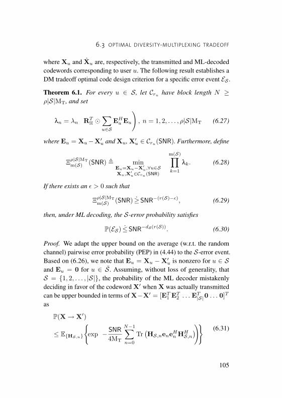
6.3 OPTIMAL DIVERSITY-MULTIPLEXING TRADEOFF
where Xu and Xu are, respectively, the transmitted and ML-decodedcodewords corresponding to user u. The following result establishes aDM tradeoff optimal code design criterion for a specific error event ES .
Theorem 6.1. For every u ∈ S, let Cru have block length N ≥ρ|S|MT, and set
λn = λn
(RT
H �∑u∈S
EHu Eu
), n = 1, 2, . . . , ρ|S|MT (6.27)
where Eu = Xu−X′u and Xu, X′u ∈ Cru(SNR). Furthermore, define
Ξρ|S|MT
m(S) (SNR) , minEu=Xu−X′u,∀u∈SXu,X
′u∈Cru (SNR)
m(S)∏k=1
λk. (6.28)
If there exists an ε > 0 such that
Ξρ|S|MT
m(S) (SNR) ≥ SNR−(r(S)−ε), (6.29)
then, under ML decoding, the S-error probability satisfies
P(ES) ≤SNR−dS(r(S)). (6.30)
Proof. We adapt the upper bound on the average (w.r.t. the randomchannel) pairwise error probability (PEP) in (4.44) to the S-error event.Based on (6.26), we note that Eu = Xu −X′u is nonzero for u ∈ Sand Eu = 0 for u ∈ S. Assuming, without loss of generality, thatS = {1, 2, . . . , |S|}, the probability of the ML decoder mistakenlydeciding in favor of the codeword X′ when X was actually transmittedcan be upper bounded in terms of X−X′ = [ET
1 ET2 . . . ET
|S|0 . . . 0]T
as
P(X→ X′)
≤ E{HS,n}
{exp
(− SNR
4MT
N−1∑n=0
Tr(HS,neneHn HH
S,n))} (6.31)
105

6 MULTIPLE-ACCESS CHANNEL
where Tr(HS,neneHn HH
S,n)
=∥∥∑
u∈SHu,neu,n∥∥2
with HS,n de-fined in (6.5) and en = [eTu1,n eTu2,n · · · eTu|S|,n]T , where eu,n =xu,n − x′u,n. Recalling HS in (6.6), we get from (6.31)
P(X→ X′)
≤ EHS
{exp(− SNR
4MTTr(HS diag
{eneHn
}N−1
n=0HHS))}
= EHw
{exp(− SNR
4MTTr(HwΥΥHHH
w
))}(6.32)
where we used HS = Hw(RT/2H ⊗I|S|MT) with Hw an MR×N |S|MT
matrix with i.i.d. CN (0, 1) entries and
Υ = (RT/2H ⊗ I|S|MT) diag{en}N−1
n=0 . (6.33)
Noting that ΥHΥ = RTH �
∑u∈S EH
u Eu and using the fact that thenonzero eigenvalues of ΥΥH in (6.32) equal the nonzero eigenvaluesof ΥHΥ, it follows, by assumption, that ΥΥH has precisely ρ|S|MT
nonzero eigenvalues. The remainder of the proof proceeds along thelines of the proof of Theorem 4.1. In particular, we split and subse-quently bound the S-error probability as
P(ES) = P(ES ,JS) + P(ES , JS)
= P(JS) P(ES |JS)︸ ︷︷ ︸≤1
+ P(JS)︸ ︷︷ ︸≤1
P(ES |JS)
≤ P(JS) + P(ES |JS) . (6.34)
As detailed in the point-to-point case, the code design criterion (6.29)yields the following upper bound on the second term in (6.34):
P(ES |JS) ≤ SNRNr(S) exp
(−SNRε/m(S)
4MT
). (6.35)
In contrast to the Jensen outage probability which satisfies P(JS) .=SNR−dS(r(S)), (6.35) decays exponentially in SNR. Hence, upon in-
106

6.3 OPTIMAL DIVERSITY-MULTIPLEXING TRADEOFF
serting (6.35) into (6.34), we get P(ES) ≤P(JS), and can thereforeconclude that P(ES) ≤SNR−dS(r(S)).
In summary, for every ES , we have a sufficient condition on {Cru :u ∈ S} for P(ES) to be exponentially upper bounded by P(JS). Note-worthily, condition (6.29) is nothing else but the code design criterionof Theorem 4.1 applied to a system operating at multiplexing rate r(S)and using |S|MT collocated antennas. However, while in the point-to-point case encoding is performed across antennas, the antennascorresponding to different users are not collocated and the correspond-ing messages have to be encoded independently. In spite of this lack ofuser cooperation at the time of communication, the families of codesCru , for all u ∈ S, can be designed in advance so as to satisfy (6.29).This task is challenging but doable as we shall see later.
Building on Theorem 6.1, we will first establish the optimal DMtradeoff of selective-fading MA channels and provide a set of codedesign criteria that guarantees optimal performance.
6.3.3. Optimal code designWe start by noting that (6.14) implies P(Or) ≥ P(OS) for any S ⊆ U ,which combined with (6.24) gives rise to 2U − 1 lower bounds onP(Or). For a given multiplexing rate tuple r, the tightest lower bound(exponentially in SNR) corresponds to the set S that yields the smallestSNR exponent dS(r(S)). More precisely, the tightest lower bound ischaracterized by
P(Or) ≥SNR−dS?(r(S?)) (6.36)
where the dominant outage event corresponds to the set
S? = arg minS ⊆ U
dS(r(S)). (6.37)
Next, we show that, for any multiplexing rate tuple, the total errorprobability Pe(Cr) can be made exponentially equal to the lower bound
107

6 MULTIPLE-ACCESS CHANNEL
in (6.36) by appropriate design of the users’ codebooks. As a directconsequence thereof, recalling from Theorem 3.5 that Pe(Cr) ≥P(Or),we then obtain that dS?(r(S?)) constitutes the optimal DM tradeoff ofthe selective-fading MA MIMO channel.
Theorem 6.2. The optimal DM tradeoff of the selective-fading MAMIMO channel in (6.1) is given by d?(r) = dS?(r(S?)), that is
d?(r) = (m(S?)− r(S?))(ρM(S?)− r(S?)). (6.38)
Moreover, if the family of codes Cr satisfies (6.29) for every S ⊆ U ,then
d(Cr) = d?(r). (6.39)
Proof. Upon inserting the upper bound (6.34) into (6.25), we get
Pe(Cr) ≤∑S⊆U
(P(JS) + P
(ES |JrS))≤∑S⊆U
P(JS) (6.40)
.= SNR−dS?(r(S?)) (6.41)
where (6.40) is a consequence of the assumption that Cr satisfies (6.29)for every S ⊆ U and (6.41) follows from (6.22) together with thedefinition (6.37). By Theorem 3.5, we have Pe(Cr) ≥P(Or) and hence,combining (6.36) and (6.41) yields
Pe(Cr) .= P(Or) .= SNR−dS?(r(S?)). (6.42)
Since, by definition, d(Cr) ≤ d?(r), using (6.13), we can concludefrom (6.42) that
d(Cr) = d?(r) = dS?(r(S?)). (6.43)
108

6.3 OPTIMAL DIVERSITY-MULTIPLEXING TRADEOFF
According to Theorem 6.2, the optimal DM tradeoff is determinedby the tradeoff curve dS?(r(S?)), which is simply the SNR exponent ofthe Jensen outage probability P(JS?) corresponding to the S?-outageevent. By virtue of (6.42) and the relations between the events OS? ,JS? , and Or, we get
P(OS?) ≤P(Or) .= P(JS?) ≤P(OS?) (6.44)
which is to sayP(OS?) .= SNR−dS?(r(S
?)). (6.45)
Hence, the Jensen upper bound on mutual information yields a boundon the S?-outage probability which is tight exponentially in SNR andconstitutes the optimal DM tradeoff. However, in order to achieve it, thefamilies of codes {Cru , u ∈ U} are required to satisfy (6.29) for everypossible subset of users S: a requirement that seems difficult to meetin general. We shall later consider an example of a code constructionwhich actually satisfies this condition in the 2-user case.
The dominant outage event determines the maximal diversity orderas a function of the multiplexing rate tuple r. Conversely, one may alsobe interested in characterizing the region of achievable multiplexingrates at a minimum diversity gain d. To this end, let us denote byrS(d) the inverse of the tradeoff curve dS(r), i.e., d = dS
(rS(d)
). If
the decay of the S-error probability is at least d over all S ⊆ U (thisimplies that all users realize a diversity requirement of d), it followsfrom Theorem 6.2 that
dS?(r(S?)) = d.
As a consequence of the definition of the dominant outage event in(6.37), we also get
dS(r(S)
) ≥ d, ∀S ⊆ U .And applying rS(·) to the both sides of the inequality yields
r(S) ≤ rS(d), ∀S ⊆ U .
109

6 MULTIPLE-ACCESS CHANNEL
We have just proved the following extension of Theorem 3.6 to selective-fading MA MIMO channels.
Corollary 6.3. Consider an overall family of codes Cr that achieves theoptimal DM tradeoff in the sense of Theorem 6.2. Then, the region ofmultiplexing rates for which a minimum diversity gain d is guaranteedto all users is characterized by
R(d) ,
{r : r(S) ≤ rS(d),∀S ⊆ U
}(6.46)
where rS(d) is the inverse function of dS(r).
This explicit characterization of R(d) generalizes the concept ofmultiplexing gain region given in (6.10) to positive diversity gains. Inorder to illustrate this point, consider the 2-user case with MT = 3,MR = 4 and ρ = 2. Figure 6.1 shows the multiplexing rate regionsR(d) corresponding to several diversity levels, i.e., d ∈ {0, 2, 4, 8, 16}.The region R(0), equivalent to the multiplexing gain region (6.10),is the pentagon described by the constraints r1 ≤ 3, r2 ≤ 3 andr1 + r2 ≤ min(4, 6) within which d ≥ 0. Larger diversity requirementcan be achieved at the expense of tighter constraints on r1 and r2. Forinstance, for a diversity requirement d ≥ 8, the multiplexing rate regionis given by the pentagon 0ABCD. Increasing the guaranteed amountof diversity results in multiplexing rate regions that shrink towards theorigin. Note that to achieve a diversity requirement d ≥ 16, the usersare required to operate at very low multiplexing rates. In this regime,the multiplexing rate region is a square: performance is not affected (inthe sense of the DM tradeoff) by the presence of a second user.
110

6.4 ERROR MECHANISMS
r1
r2
1
21
3
3
2
d ! 0
d ! 2
d ! 4
d ! 8
d ! 16
0D
C
BA
Fig. 6.1: Multiplexing rate regions as a function of the minimum diversityrequirement d ∈ {0, 2, 4, 8, 16} for both users (MT = 3, MR = 4 andρ = 2). The diversity gain d corresponding to any multiplexing rate tupleinside the pentagon 0ABCD satisfies d ≥ 8.
6.4 . ERROR MECHANISMS
The error exponent analysis conducted by Gallager (1985) for theAWGN MA channel can be extended to selective-fading MA MIMOchannels, e.g., see (Gärtner and Bölcskei, 2006) in the context of fixeddata rates. In this section, we review the concept of dominant errorevent, which is central to the error exponent framework, and show howit carries over into the DM tradeoff framework. We shall also see thatthe dominant error event leads to an accurate characterization of themechanisms of error in selective-fading MA MIMO channels.
111

6 MULTIPLE-ACCESS CHANNEL
6.4.1. PreliminariesThe capacity region contains all the rate tuples (R1, R2, . . . , RU ) thatcan be transmitted through the channel with vanishing probability oferror as the block length grows to infinity. Similar to the study oferror exponents in the point-to-point case (Gallager, 1968), the errorexponent analysis conducted by Gallager (1985) for the AWGN MAchannel aims at quantifying the decay of the error probability with blocklength as a function of the rate tuple (R1, R2, . . . , RU ) in the capacityregion. Gallager focuses on the 2-user case, and finds that, dependingon the tuple (R1, R2), the total error probability is either dominated bysingle-user errors, i.e., only one of the two users is decoded incorrectly,or by a joint error, i.e., both users are simultaneously decoded in error.This distinction gives rise to the notion of error events types, which, inour analysis, are referred to as S-error events, and justifies the followingdecomposition of the error probability
P(E) = P(E1) + P(E2) + P(E3)
where E1 corresponds to user 1 only being in error, E2 to user 2 onlybeing in error, and E3 is the event of both users being simultaneouslyin error (note that we have used a similar decomposition of the errorprobability in (6.25)). The findings of Gallager show that the dominanttype of error, or dominant error event, corresponds to the term withthe smallest random coding exponent, i.e., the term with the slowestexponential decay with block length. Moreover, the achievable rateregion can be separated into three distinct areas, each one dominatedby a different error event.
6.4.2. Dominant error eventIn the context of the DM tradeoff the problem is conceptually similarto that addressed by Gallager: we aim at identifying the S-error eventthat dominates the total error probability as the SNR (and not the blocklength) grows to infinity. We summarize our result as follows.
112

6.4 ERROR MECHANISMS
Theorem 6.4. Under the assumptions of Theorem 6.2, the total errorprobability satisfies
Pe(Cr) .= P(ES?) . (6.47)
where the set S?, defined in (6.37), corresponds to the dominant S-outage event for the multiplexing rate tuple r.
Proof. Let ES′ denote the S-error event that dominates the overall errorprobability so that, based on (6.25),
Pe(Cr) .= P(ES′) .By (6.42), we necessarily have dS?(r(S?)) = d(ES′), where
d(ES′) = − limSNR→∞
log P(ES′)log SNR
.
Since Cr satisfies (6.29) ∀S ⊆ U , Theorem 6.1 yields d(ES′) ≥dS′(r(S ′)) and, hence, we get
dS?(r(S?)) ≥ dS′(r(S ′)).However, by the definition of S?, we also have dS?(r(S?)) ≤ dS′(r(S ′))which implies dS?(r(S?)) = dS′(r(S ′)). We can hence conclude thatPe(Cr) .= P(ES?).
The optimal DM tradeoff is therefore given by the SNR exponentcorresponding to the dominant error event, which is to say that theconcept of dominant error event carries over in the context of the DMtradeoff. This fact is remarkable since, except for interference, errorsover the fading MA channel are mainly due to channel outage whilein the original AWGN MA channel errors were exclusively due toatypically large noise realizations.
The following example illustrates the application of Theorem 6.2to the two-user case, and reveals multiplexing rate regions dominatedby different error events. Noteworthily, despite being obtained in adrastically different setting, our regions resemble Gallager’s dominatingerror regions for the AWGN MA channel case.
113
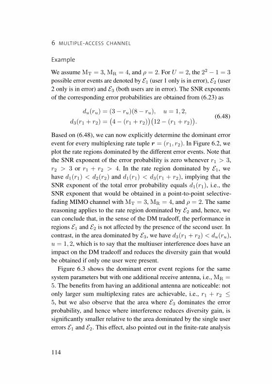
6 MULTIPLE-ACCESS CHANNEL
Example
We assume MT = 3, MR = 4, and ρ = 2. For U = 2, the 22 − 1 = 3possible error events are denoted by E1 (user 1 only is in error), E2 (user2 only is in error) and E3 (both users are in error). The SNR exponentsof the corresponding error probabilities are obtained from (6.23) as
du(ru) = (3− ru)(8− ru), u = 1, 2,
d3(r1 + r2) =(4− (r1 + r2)
)(12− (r1 + r2)
).
(6.48)
Based on (6.48), we can now explicitly determine the dominant errorevent for every multiplexing rate tuple r = (r1, r2). In Figure 6.2, weplot the rate regions dominated by the different error events. Note thatthe SNR exponent of the error probability is zero whenever r1 > 3,r2 > 3 or r1 + r2 > 4. In the rate region dominated by E1, wehave d1(r1) < d2(r2) and d1(r1) < d3(r1 + r2), implying that theSNR exponent of the total error probability equals d1(r1), i.e., theSNR exponent that would be obtained in a point-to-point selective-fading MIMO channel with MT = 3, MR = 4, and ρ = 2. The samereasoning applies to the rate region dominated by E2 and, hence, wecan conclude that, in the sense of the DM tradeoff, the performance inregions E1 and E2 is not affected by the presence of the second user. Incontrast, in the area dominated by E3, we have d3(r1 + r2) < du(ru),u = 1, 2, which is to say that the multiuser interference does have animpact on the DM tradeoff and reduces the diversity gain that wouldbe obtained if only one user were present.
Figure 6.3 shows the dominant error event regions for the samesystem parameters but with one additional receive antenna, i.e., MR =5. The benefits from having an additional antenna are noticeable: notonly larger sum multiplexing rates are achievable, i.e., r1 + r2 ≤5, but we also observe that the area where E3 dominates the errorprobability, and hence where interference reduces diversity gain, issignificantly smaller relative to the area dominated by the single usererrors E1 and E2. This effect, also pointed out in the finite-rate analysis
114

6.5 OPTIMAL DISTRIBUTED SPACE-TIME CODING
0 1 2 30
1
2
3
0 1 2 30
1
2
3
Fig. 6.2: Dominant error event regions for the two-user MA MIMO channelwith MT = 3, MR = 4, and ρ = 2.
of (Gärtner and Bölcskei, 2006), can be intuitively explained by thefact that increasing MR yields more spatial degrees of freedom at thereceiver and, consequently, it alleviates the task of discriminating theusers’ signals in a larger portion of the multiplexing rate region. Fora small set of high multiplexing rates, however, the joint error stilldominates the error probability.
6.5. OPTIMAL DISTRIBUTED SPACE-TIMECODING
Satisfying the code design criterion (6.29) for every S ⊆ U is non-trivial and systematic procedures for designing DM tradeoff optimalcodes are an important open problem. In this section, we show that the
115

6 MULTIPLE-ACCESS CHANNEL
0 1 2 30
1
2
3
0 1 2 30
1
2
3
Fig. 6.3: Dominant error event regions for the two-user MA MIMO channelwith MT = 3, MR = 5, and ρ = 2.
algebraic code construction proposed recently by Badr and Belfiore(2008b) for flat-fading MA channels with single-antenna users satisfies(6.29) for every S ⊆ U and any multiplexing rate tuple∗.
We start by briefly reviewing the code construction described inBadr and Belfiore (2008b) for a system with MT = 1, MR = 2,U = 2, N = 2, and ρ = 1. For each user u, let Au denote a QAMconstellation with 2Ru(SNR) points carved from Z[i] = {k + il : k, l ∈Z}, where i =
√−1. The proposed code spans two slots so that thevector of information symbols corresponding to user u is given by su =[su,0 su,1], where su,0, su,1 ∈ Au. Using the unitary transformationmatrix U underlying the Golden Code (Belfiore et al., 2005), the 1× 2
∗In (Badr and Belfiore, 2008b), the DM tradeoff optimality of the proposed code isshown for r1 = r2.
116

6.5 OPTIMAL DISTRIBUTED SPACE-TIME CODING
codeword Xu is obtained as
XTu = U sTu =
[xu
σ(xu)
](6.49)
with the matrix U given by
U =1√5
[α αϕ
α αϕ
](6.50)
where ϕ = 1+√
52 denotes the Golden number with corresponding
conjugate ϕ = 1−√52 , α = 1 + i − iϕ and α = 1 + i − iϕ. Here, σ
denotes the generator of the Galois group of the quadratic extensionQ(i,√
5) over Q(i) = {k + il : k, l ∈ Q} given by
σ : Q(i,√
5) → Q(i,√
5)a+ b
√5 7→ a− b√5.
(6.51)
Moreover, one of the users, say user 2, multiplies the symbol corre-sponding to the first slot by a constant γ ∈ Q(i), resulting in the overall2× 2 codeword
X =[x1 σ(x1)γx2 σ(x2)
]. (6.52)
As shown in (Badr and Belfiore, 2008b), for any γ 6= ±1 and anytwo X,X′ according to (6.52), it holds that det(∆) 6= 0, where ∆ =X−X′. For the so-defined construction we have the following result.
Theorem 6.5. For any multiplexing rate tuple r, the algebraic codeconstruction in (Badr and Belfiore, 2008b) satisfies (6.29) for anyS ⊆ U .
Proof. For completeness, we start by proving that the determinantcorresponding to any codeword X in (6.52) is nonzero for any γ 6=±1, and hence, by the linearity of the mapping σ over Q(i,
√5), the
117

6 MULTIPLE-ACCESS CHANNEL
determinant of any codeword difference matrix is also nonzero. Notethat
det(X) = x1σ(x2)− γx2σ(x1)
= x− γσ(x) (6.53)
where last step follows from setting x = x1σ(x2) and using the prop-erty σ(x ·y) = σ(x) ·σ(y) for every x, y ∈ Q(i,
√5). Hence, the deter-
minant is zero if and only if γ satsifies γ = x/σ(x). In this case, recall-ing that γ ∈ Q(i), we must have x ∈ Q(i), or x ∈ √5Q(i). These con-straints yield, respectively, γ = x/σ(x) = 1 and γ = x/σ(x) = −1,from which we can conclude that det(X) = 0 ⇐⇒ γ = ±1. Hence,any γ ∈ Q(i)\{±1} yields a nonzero determinant.
We consider now the second part of the proof. Assume that at anygiven SNR, user u carves out 2Ru(SNR)−ε log SNR points from Z[i] forsome ε > 0, i.e., |Au| = SNRru−ε. In order to satisfy the power con-straint (6.2), we scale Au by SNR−(ru−ε)/2 so that, due to the linearity(over C) of the transformation in (6.49), the codeword correspondingto user u is given by SNR−(ru−ε)/2 Xu. From (6.52) and the linearityof the mapping σ over Q(i,
√5), the codeword difference matrix is
obtained as
E =
[SNR−(r1−ε)/2e1 SNR−(r1−ε)/2σ(e1)SNR−(r2−ε)/2γe2 SNR−(r2−ε)/2σ(e2)
](6.54)
where eu = xu−x′u, u = 1, 2. Next, we note that in the flat-fading caseRT
H �EHE = EHE. In particular, considering user 1, i.e., S = {1},we have |S| = 1 and m(S) = 1 so that, from (6.28), we obtain
Ξ11(SNR) = SNR−(r1−ε) min
e1(|e1|2 + |σ(e1)|2). (6.55)
Letting XT1 = UsT1 and (X′1)T = U(s′1)T and using the fact that U
is unitary, we get
(|e1|2 + |σ(e1)|2) = ||s1 − s′1||2 ≥ 2d2min (6.56)
118

6.5 OPTIMAL DISTRIBUTED SPACE-TIME CODING
where dmin is the (nonzero and SNR-independent) minimum distancein A1. We therefore conclude that Ξ1
1(SNR) .= SNR−(r1−ε). For user2, a similar argument shows that Ξ1
1(SNR) .= SNR−(r2−ε) and, hence,the construction satisfies the criteria arising from (6.29) for S = {1}and S = {2}.
For S = {1, 2}, note that |S| = 2 and m(S) = 2 so that
Ξ22(SNR) = min
E|det(E)|2 . (6.57)
From (6.54), we get
|det(E)|2 = SNR−(r1+r2−2ε) |det(∆)|2 . (6.58)
Recalling that for any γ 6= ±1, det(∆) is nonzero and independent ofSNR, it follows that |det(E)|2 .= SNR−(r1+r2−2ε) and, consequently,we obtain
Ξ22(SNR) .= SNR−(r1+r2−2ε) (6.59)
from which we can conclude that (6.29) is also satisfied for S ={1, 2}. The proof is concluded by taking ε to be arbitrarily close tozero, implying that both users operate arbitrarily close to their targetmultiplexing rates.
Other code constructions that achieve the optimal DM tradeoff offlat-fading channels were recently reported in (Nam and El Gamal,2007; Badr and Belfiore, 2008a). In Nam and El Gamal (2007), it isshown that lattice-based space-time codes achieve the optimal DMtradeoff with lattice decoding. Badr and Belfiore (2008a), on the otherhand, extend the construction considered in this section to the caseof multiple antennas at the users’ transmitters. However, we note thatthe problem of systematically constructing DM tradeoff optimal codesseems to remain largely unexplored in the case of selective-fading MAMIMO channels.
119


CHAPTER 7
Conclusion
THIS DISSERTATION provides a high-SNR characterization ofthe optimal rate-reliability tradeoff for communication systemsoperating over selective-fading wireless channels. Our analysis
and results are presented in the diversity-multiplexing (DM) tradeoffframework (Zheng and Tse, 2003), in which rate and reliability arerespectively captured by the concepts of multiplexing and diversity.
The principal difficulty we overcome to establish the optimal DMtradeoff for selective-fading channels is of technical nature: the mutualinformation for this class of channels is in general a sum of correlatedrandom variables whose distribution is unknown. Nevertheless, we areable to carry our analysis through by introducing the “Jensen channel”,that is, a conceptual channel associated with the original channel andwhich behaves likewise in the high-SNR regime. The Jensen channelturns out to be a very useful tool not only in the context of point-to-point channels and multiple-access (MA) channels addressed in thisthesis, but also, as evidenced by the work of Akçaba et al. (2007), inanalyzing ultimate communication performance in the relay channel.
The proof techniques employed in this thesis reveal code design cri-teria that guarantee optimal performance in both the point-to-point caseand the MA case. We also establish the existence of codes satisfyingthese criteria by providing examples of optimal constructions.
121

7 CONCLUSION
In the point-to-point case, we show that the problem of constructingoptimal codes can be split into two simpler and independent tasks: theconstruction of a precoder, or inner code, which takes explicitly intoaccount the channel’s selectivity characteristics, and the constructionof an outer code which is independent of the channel. This thesispresents a simple procedure, which is a generalization of the well-established phase- and delay-diversity techniques, to construct theprecoder based on the channel’s covariance matrix. We show thatthe permutation codes over quadrature amplitude modulation (QAM)constellations introduced by Tavildar and Viswanath (2006) can beused in conjunction with our precoder to achieve optimal performance.Identifying additional outer codes that could be used with our precoderwould be an interesting aspect to consider in future research.
We also show that the code construction for the two-user MA chan-nel presented in (Badr and Belfiore, 2008b) satisfies our code designcriteria. However, more work is still needed to address the problemof constructing optimal codes for the general MA channel. A possibleavenue to explore would be to extend our systematic code construc-tion procedure to the MA channel, i.e., to jointly develop the users’precoders and corresponding outer codes in order to satisfy the designcriteria. While the precoder design technique presented in this thesisseems to be readily extendable to multiple users, it is still unclear howto design the users’ outer codes.
Finally, this thesis also presents an interesting relation between theDM tradeoff framework in MA channels and the concept of dominanterror event which was first introduced by Gallager (1985) for additivewhite Gaussian noise (AWGN) MA channels. The idea is that a de-coding error can be decomposed into several disjoint error events ofwhich only one dominates the error probability asymptotically in SNR.Extending this concept to additional communication channels in futurework seems promising, and it might lead to a more comprehensiveunderstanding of the error mechanisms in wireless communication.
122

APPENDIX A
Linear Frequency-Invariant and LinearTime-Invariant Systems
This appendix examines the input-output relation over linear frequency-invariant (LFI) and linear time-invariant (LTI) channels. These channelscan be thought of as limiting cases of a linear time-varying (LTV) sys-tem with vanishing delay spread or vanishing Doppler spread, respec-tively. Although LFI and LTI channel operators have a well-structuredset of eigenfunctions (complex sinusoids for LTI systems and Diracfunctions parametrized by time for LFI systems), their diagonalizationcannot be casted in terms of the general underspread LTV frameworkpresented in Chapter 2 (Durisi et al., 2008, Sec. II.C).
LFI and LTI systems are rather popular models to describe wirelesschannels in the communication engineering literature (e.g., Proakis,2001; Tse and Viswanath, 2005). It is therefore interesting to note thatthe input-output relation used throughout this thesis, i.e.,
yn =√
SNR hn xn + zn, n = 0, 1, . . . , N − 1, (A.1)
is also applicable to describe communication over this class of channels.We consider here the case of scalar channels, but the discussion readilyextends to multiple-antenna channels.
123

A LINEAR FREQUENCY-INVARIANT AND LINEAR TIME-INVARIANT SYSTEMS
In the case of an LTI channel, the input-output relation (A.1) canbe obtained by using an orthogonal frequency-division multiplexing(OFDM) system (Peled and Ruiz, 1980) with N tones. Assuming thatthe OFDM system employs a cyclic prefix (guard interval) exceedingthe channel’s delay spread, the effect of the LTI channel on the transmitsignal is described in terms of a cyclic (instead of linear) convolution.Then, applying appropriate Fourier transforms to the signal at thetransmitter and at the receiver, the original frequency-selective channelis transformed into N non-interfering subchannels as in (A.1). In thecase of an LFI channel, the input-ouput relation (A.1) can be obtainedby employing a basis expansion model (BEM) (Ma et al., 2005).
The channel covariance matrix corresponding to (A.1) is obtained asfollows. Suppose that {h(l)}L−1
l=0 are L channel samples taken eitherin the delay domain for an LTI system, or in the Doppler frequencydomain for an LFI system. Note that the resolution L depends upon theinput signal bandwidth (LTI system), or upon the output signal duration(LFI system). For the two approaches considered above, the channel isdescribed by
hn =L−1∑l=0
h(l) e−j2πN ln, n = 0, 1, . . . , N − 1,
where the h(l) have i.i.d. CN (0, σ2l
)entries and satisfy
E{h(l)h∗(l′)} = σ2l δ(l − l′).
The samples are uncorrelated due to the uncorrelated scattering (US)assumption for the LTI channel, and due to the wide-sense stationary(WSS) assumption for the LFI channel. Then, the channel’s covariancematrix clearly follows as
RH = Ψ diag{σ2
0 , σ21 , . . . , σ
2L−1, 0, . . . , 0
}ΨH (A.2)
where Ψ, Ψ(i, j) = 1√Ne−j
2πN ij (i, j = 0, 1, . . . , N − 1), denotes the
N ×N Fourier matrix.
124

APPENDIX B
Distribution of the Jensen Channel
We show that the Jensen channel satisfies H = Hw(RT/2 ⊗ IM),where{
R = RH, Hw = [Hw,0 Hw,1 · · · Hw,N−1] if MR ≤ MT,
R = RTH , Hw = [HH
w,0 HHw,1 · · · HH
w,N−1] if MR > MT.(B.1)
We start by considering the case MR ≤ MT, where, recalling (4.22),the Jensen channel is simply given by H = [H0 H1 · · · HN−1]. By(4.5), it follows that E{vec (H) vec (H)H} = RH ⊗ IMTMR so that,using M = MT, we may write H = Hw(RT/2
H ⊗ IM). PartitioningHw into blocks of size MR × MT readily yields (B.1) for the caseMR ≤ MT.
In the case MR > MT, we set RT/2H (n, n′) = rn,n′ for the sake of
notation, and note that the following equality holds for every realizationof the channel:
[H0 H1 · · · HN−1] = [Hw,0 Hw,1 · · · Hw,N−1](RT/2
H ⊗ IMT
)=N−1∑n=0
[rn,0Hw,n rn,1Hw,n · · · rn,N−1Hw,n].
125

B DISTRIBUTION OF THE JENSEN CHANNEL
Next, we use this observation to write
H = [HH0 HH
1 · · · HHN−1]
=N−1∑n=0
[r∗n,0HHw,n r
∗n,1H
Hw,n · · · r∗n,N−1H
Hw,n]
= [HHw,0 HH
w,1 · · · HHw,N−1]
((RT/2
H )∗ ⊗ IMR
). (B.2)
Since R1/2H is the positive semidefinite square root of RH = UΛUH ,
we have
(RT/2H )∗ =
((UΛ1/2UH)T
)∗= (U∗Λ1/2UT )∗
= UΛ1/2UH = R1/2H
which, combined with (B.2) and M = MR, yields
H = [HHw,0 HH
w,1 · · · HHw,N−1](R1/2
H ⊗ IM)
hence establishing (B.1) for the case MR > MT.
126

APPENDIX C
Worst Pairwise Distance
The pairwise distance between two possible codewords takes the formTr(BABH
), where A is Hermitian and B diagonalizable. This ap-
pendix provides a lower bound to Tr(BABH
)in terms of the eigen-
values of A and B. This result is proved in (Köse and Wesel, 2003,Theorem 2) for the case of a square matrix B.
Suppose that A is a n× n Hermitian matrix and let its eigenvaluedecomposition be given by
A = UΘUH (C.1)
with Θ = diag{θl}nl=1, θ1 ≤ θ2 ≤ . . . ≤ θn, and U ∈ Tn, where Tndenotes the set of unitary matrices of size n. Moreover, let the singularvalue decomposition of the m× n matrix B be given by
B = VΛ1/2WH (C.2)
where V ∈ Tm, W ∈ Tn, and Λ has zeros in its off-diagonal entriesbut [Λ]k,k = λk for k = 1, 2, . . . ,m, with λ1 ≤ λ2 ≤ . . . ≤ λp andp , min(m,n). Then, we have the following theorem.
Theorem C.1. For A and B given respectively by (C.1) and (C.2), wehave
minU,W∈Tn
Tr(BABH
)=
p∑k=1
λk θp+1−k.
127

C WORST PAIRWISE DISTANCE
Proof. Set Q = WHU, with Q ∈ Tn, and note that using (C.1) and(C.2), we get
minU,W∈Tn
Tr(BABH
)= min
Q∈TnTr(Λ1/2 Q Θ QHΛ1/2
)= min
Q∈Tn
p∑k=1
λk
n∑l=1
|Q(k, l)|2 θl
≥ minD∈Dn
p∑k=1
λk
n∑l=1
D(k, l) θl (C.3)
where D, defined by D(k, l) = |Q(k, l)|2, is doubly stochastic, Dn ⊃Tn denotes the set of doubly stochastic matrices of size n, and (C.3)is direct consequence of enlarging the set of admissible matrices toinclude doubly stochastic matrices. Since Dn is a convex compact setand (C.3) is a linear function of D(k, l), the minimum is attained at anextreme point of the set. By Birkhoff’s Theorem (Horn and Johnson,1993, 8.7.1), which says that the extreme points of Dn are permutationmatrices P, we have
minD∈Dn
p∑k=1
λk
n∑l=1
D(k, l) θl = minP
p∑k=1
λk
n∑l=1
P(l, k) θl
= minπ
p∑k=1
λk θπ(k) (C.4)
=p∑k=1
λk θp+1−k (C.5)
where (C.4) follows from the structure of P, i.e., one entry per rowis equal to one and the rest are zeros, π denotes a permutation on{1, 2, . . . , n}, and (C.5) is a direct consequence of the ordering as-sumed for the λk’s and θl’s. The proof is concluded by noting thatpermutation matrices do also belong to Tn, i.e., the initial set of ad-missible matrices, and, hence, the minimum in (C.5) is attained withequality.
128

APPENDIX D
Notation
D.1 . SYSTEM
MT,MR number of transmit and receive antennasm,M min(MT,MR) and max(MT,MR)R,R(SNR) data rate and SNR-dependent data rateU set of users U = {1, 2, . . . , U}S subset of users in U|S| cardinality of SS complement of S in Um(S) min(|S|MT,MR)M(S) max(|S|MT,MR)(R1, R2, . . . , RU ) data rate tuple
129

D NOTATION
D.2. DIVERSITY-MULTIPLEXING TRADEOFF
Point-to-point channel
r multiplexing rateEr error event at multiplexing rate rOr outage event at multiplexing rate rJr Jensen outage event at multiplexing rate rCr family of codes operating at multiplexing rate rCr(SNR) codebook in Cr corresponding to SNR
Pe(Cr) error probability corresponding to CrdO SNR exponent of the outage probabilitydJ SNR exponent of the Jensen outage probabilityd? optimal diversity-multiplexing tradeoff over all CrH [H0 H1 · · · HN−1]H Jensen channelI(SNR) mutual information for i.i.d. Gaussian inputJ(SNR) Jensen upper bound on I(SNR)
130

D.2 DIVERSITY-MULTIPLEXING TRADEOFF
Multiple-access channel
r multiplexing rate tuple (r1, r2, . . . , rU )r(S) total multiplexing rate corresponding to the users in
S ⊆ U , i.e., r(S) =∑u∈S ru
ES S-error eventOS S-outage eventJS Jensen outage event corresponding to SOr outage set w.r.t. the multiplexing rate tuple rCr overall codebook Cr1 × Cr2 × · · · × CrUPe(Cr) error probability of CrdS SNR exponent of P(JS)d? optimal diversity-multiplexing tradeoff over all CrHS Jensen channel of S = {u1, u2, . . . , u|S|}HS,n [Hu1,n Hu2,n · · · Hu|S|,n]HS [HS,0 HS,1 · · · HS,N−1]IS(SNR) sum mutual information for users in SJS(SNR) Jensen upper bound on IS(SNR)
General
SNR (per-user) average SNR at each receive antenna.= exponential equality: two functions f(x) and g(x) are
said to be exponentially equal if and only iflimx→∞
log f(x)log x = limx→∞
log g(x)log x .
≤, ≥ exponential inequality<, > strict exponential inequalityPout(R) outage probability at rate RPJ(R) Jensen outage probability at rate Rλn nonzero eigenvalues of the effective codeword
difference matrix, i.e., λk = λk(RTH �EHE)
Ξmn product of the n smallest eigenvalues of m nonzeroeigenvalues λ1, λ2, . . . , λm
131

D NOTATION
D.3. LINEAR ANALYSIS
A,a, a matrix, column vector, and row vectorA(i, j),a(i) (i, j)th entry of A, ith entry of aAT ,AH transposition and conjugate transposition of AA∗ element-wise conjugationA⊗B Kronecker product of A and BA�B Hadamard product of A and Bvec(A) if ak (k=1, 2, . . . ,m) are the columns of A,
then vec(A) = [aT1 aT2 . . . aTm]T
Tr (A) trace of A, i.e., Tr (A) =∑i A(i, i)
‖A‖2F squared Frobenius norm, i.e.,‖A‖2F = Tr
(AAH
)‖x‖ norm of the vector xdet(A) determinant of a nonsingular matrix, i.e.,∏
i λi(A)rank(A) rank of Adiag{An}N−1
n=0 block diagonal matrix obtained by diagonallystacking A0,A1, . . . ,AN−1
Da diag{a(n)}N−1n=0
A1/2 positive semidefinite square root of an Hermitianmatrix A
A(I1, I2) (sub)matrix consisting of the rows of A indexedby I1 and the columns of A indexed by I2
λk(A) nonzero eigenvalues of the n× n Hermitianmatrix A, sorted in ascending order(k = 1, 2, . . . , rank(A))
F,Ψ,Φ Fourier matrices (F = Ψ⊗Φ is two-level)1N N ×N all-ones matrixΠ basic circulant permutation [π1 · · · πN−1 π0],
where πn = [0 · · · 0 1 0 · · · 0]T contains a 1 inits nth position.
132

D.4 PROBABILITY AND STATISTICS
D. 4 . PROBABILITY AND STATISTICS
P(A) probability of the event AP(A,B) joint probability of A and BP(A |B) conditional probability of A given BfX(x) probabiltiy density function (pdf) of XX ∼ Y equality in distribution of X and Yfx, f(X) pdf of the random vector x or matrix XE{·} expectation operatorEX{·} expectation operator with respect to Xx ∼ CN (µ,C) jointly proper Gaussian (JPG) random vector
with mean µ and covariance matrix Cx ∼ N (µ, σ2
)real Gaussian random variable with mean µ andvariance σ2
D.5 . MISCELLANEOUS
R set of real numbersQ set of rational numbersZ set of integersN set of naturalsC set of complex numbersRe(x) real part of complex number xIm(x) imaginary part of complex number xδn,m Kronecker delta function, i.e., δn,m = 1 for n = m
and zero otherwiseδ(t) Dirac distributionF Fourier operator|x| absolute value of x ∈ R, or magnitude of x ∈ CQ(x) Gaussian tail function Q(x) = 1√
2π
∫∞xe−t
2/2dt
133


APPENDIX E
Acronyms and abbreviations
AWGN additive white Gaussian noiseCSI channel state informationDM diversity-multiplexingFEC forward error correctionICI intercarrier interferenceISI intersymbol interferenceJPG jointly proper GaussianLFI linear frequency-invariantLTI linear time-invariantLTV linear time-varyingML maximum-likelihoodMA multiple-accessMIMO multiple-input multiple-outputOFDM orthogonal frequency-division multiplexingQAM quadrature amplitude modulationQoS quality-of-serviceSNR signal-to-noise ratioSISO single-input single-ouputWSSUS wide-sense stationary uncorrelated scatteringw.p. 1 with probability 1w.r.t. with respect to
135


References
Adachi, F. (1979), “Transmitter diversity for a digital FM paging system,” IEEETrans. Veh. Technol., vol. 28, pp. 333–338.
Ahlswede, R. (1971), “Multi-way communication channels,” in 2nd Int. Symp.Inf. Theory (Tsahkadsor, Armenian S.S.R.), pp. 23–52, Budapest: Hungar-ian Academy of Sciences.
Akçaba, C., Kuppinger, P., and Bölcskei, H. (2007), “Distributed transmitdiversity in relay networks,” in IEEE Information Theory Workshop (ITW),pp. 233–237, Bergen, Norway.
Alamouti, S. M. (1998), “A simple transmit diversity technique for wirelesscommunications,” IEEE J. Sel. Areas Commun., vol. 16, no. 8, pp. 1451–1458.
Badr, M. and Belfiore, J.-C. (2008a), “Distributed space-time block codes forthe MIMO multiple access channel,” in Proc. IEEE Int. Symp. Inf. Theory(ISIT), pp. 2553–2557, Toronto, ON, Canada.
——— (2008b), “Distributed space-time block codes for the non cooperativemultiple access channel,” in Proc. Int. Zurich Seminar on Commun., pp.132–135.
Belfiore, J.-C. and Rekaya, G. (2003), “Quaternionic lattices for space-timecoding,” in Proc. IEEE Inf. Theory Workshop, pp. 267–270, Paris, France.
Belfiore, J.-C., Rekaya, G., and Viterbo, E. (2005), “The Golden code: A 2× 2full rate space-time code with nonvanishing determinants,” IEEE Trans.Inf. Theory, vol. 51, no. 4, pp. 1432–1436.
Bello, P. A. (1963), “Characterization of randomly time-variant linear channels,”IEEE Trans. Commun. Syst., vol. COM-11, pp. 360–393.
Biglieri, E. (2005), Coding for Wireless Channels, New York, NY: Springer.Bölcskei, H., Borgmann, M., and Paulraj, A. J. (2003a), “Impact of the propa-
137

REFERENCES
gation environment on the performance of space-frequency coded MIMO-OFDM,” IEEE J. Select. Areas Commun., vol. 21, no. 3, pp. 427–439.
——— (2003b), “Space-frequency coded MIMO-OFDM with variablemultiplexing-diversity tradeoff,” in Proc. IEEE Int. Conf. Commun. (ICC),pp. 2837–2841, Anchorage, AK.
Bölcskei, H., Gesbert, D., and Paulraj, A. J. (2002a), “On the capacity ofOFDM-based spatial multiplexing systems,” IEEE Trans. Commun.,vol. 52, no. 2, pp. 225–234.
Bölcskei, H., Koetter, R., and Mallik, S. (2002b), “Coding and modulationfor underspread fading channels,” in Proc. IEEE Int. Symp. Inf. Theory(ISIT), p. 358, Lausanne, Switzerland.
Bölcskei, H. and Paulraj, A. J. (2000), “Space-frequency coded broadbandOFDM systems,” in Proc. IEEE Wireless Commun. Net. Conf. (WCNC),pp. 1–6, Chicago, IL.
Boutros, J. and Viterbo, E. (1998), “Signal space diversity: A power- andbandwidth-efficient diversity technique for the rayleigh fading channel,”IEEE Trans. Inf. Theory, vol. 44, no. 4, pp. 1453–1467.
Coronel, P. and Bölcskei, H. (2007), “Diversity-multiplexing tradeoff inselective-fading MIMO channels,” in Proc. IEEE Int. Symp. Inf. The-ory (ISIT), pp. 2841–2845, Nice, France.
Coronel, P., Gärtner, M., and Bölcskei, H. (2008), “Diversity-multiplexingtradeoff in selective-fading multiple-access MIMO channels,” in Proc.IEEE Int. Symp. Inf. Theory (ISIT), pp. pp. 915–919, Toronto, ON,Canada.
Cover, T. M. and Thomas, J. A. (1991), Elements of Information Theory, NewYork, NY: Wiley, 2nd ed.
Dayal, P. and Varanasi, M. K. (2005), “An optimal two transmit antenna space-time code and its stacked extensions,” IEEE Trans. Inf. Theory, vol. 51,no. 12, pp. 4348–4355.
Divsalar, D. and Simon, M. K. (1988), “The design of trellis coded MPSK forfading channels: Performance criteria,” IEEE Trans. Commun., vol. 36,no. 9, pp. 1004–1012.
Durisi, G., Schuster, U. G., Bölcskei, H., and Shamai (Shitz), S. (2008), “Nonco-herent capacity of underspread fading channels,” IEEE Trans. Inf. Theory.Submitted. [Online]. Available: http://arxiv.org/abs/0804.1748.
Edelman, A. (1989), Eigenvalues and condition number of random matrices,Ph.D. thesis, Department of Mathematics, Massachusetts Institute ofTechnology, Cambridge, MA.
138

REFERENCES
El Gamal, H., Caire, G., and Damen, M. O. (2004), “Lattice coding anddecoding achieves the optimal diversity-multiplexing tradeoff of MIMOchannels,” IEEE Trans. Inf. Theory, vol. 50, no. 9, pp. 968–985.
Elia, P., Kumar, K. R., Pawar, S. A., Kumar, P. V., and Lu, H.-F. (2006), “Ex-plicit space-time codes achieving the diversity-multiplexing gain tradeoff,”IEEE Trans. Inf. Theory, vol. 52, no. 9, pp. 3869–3884.
Foschini, G. J. (1996), “Layered space-time architecture for wireless communi-cation in a fading environment when using multi-element antennas,” BellLabs Tech. J., vol. 1, no. 2, pp. 41–59.
Gallager, R. G. (1968), Information Theory and Reliable Communication, NewYork, NY: Wiley.
——— (1985), “A perspective on multiaccess channels,” IEEE Trans. Inf.Theory, vol. 31, no. 2, pp. 124–142.
Gärtner, M. and Bölcskei, H. (2006), “Multiuser space-time/frequency codedesign,” in Proc. IEEE Int. Symp. Inf. Theory (ISIT), pp. 2819–2823,Seattle, WA.
Gray, R. M. (2006), “Toeplitz and circulant matrices: A review,” Foundationsand Trends in Communications and Information Theory, vol. 2, no. 3, pp.155–239.
Grokop, L. and Tse, D. N. C. (2004), “Diversity/multiplexing tradeoff in ISIchannels,” in Proc. IEEE Int. Symp. Inf. Theory (ISIT), p. 96, Chicago,USA.
Guey, J., Fitz, M., Bell, M., and Kuo, W. (1999), “Signal design for transmitterdiversity wireless communication systems over Rayleigh fading channels,”IEEE Trans. Commun., vol. 47, no. 4, pp. 527–537.
Harashima, H. and Miyakawa, H. (1972), “Matched-transmission technique forchannels with intersymbol interference,” IEEE Trans. Commun., vol. 20,pp. 774–780.
Hiroike, A., Adachi, F., and Nakajima, N. (1992), “Combined effects of phasesweeping transmitter diversity and channel coding,” IEEE Trans. Veh.Technol., vol. 41, no. 2, pp. 170–176.
Horn, R. A. and Johnson, C. R. (1993), Matrix Analysis, Cambridge UniversityPress, 2nd ed.
Jakes, W. (1974), Microwave mobile communications, New York, NY: Wiley.James, A. T. (1964), “Distribution of matrix variates and latent roots derived
from normal samples,” Annals of Mathematical Statistics, vol. 35, pp.475–501.
139

REFERENCES
Jensen, J. L. W. V. (1906), “Sur les fonctions convexes et les inégalités entreles valeurs moyennes,” Acta Math., vol. 30, no. 1, pp. 175–193.
Kaiser, S. (2000), “Spatial transmit diversity techniques for broadband OFDMsystems,” in Proc. IEEE Global Telecommun. Conf. (GLOBECOM’00),vol. 3, pp. 1824–1828.
Köse, C. and Wesel, R. D. (2003), “Universal space-time trellis codes,” IEEETrans. Inf. Theory, vol. 49, no. 10, pp. 2717–2727.
Kozek, W. (1997), Matched Weyl-Heisenberg expansions of nonstationaryenvironments, Ph.D. thesis, Vienna University of Technology.
Kozek, W. and Molisch, A. F. (1998), “Nonorthogonal pulseshapes for mul-ticarrier communications in doubly dispersive channels,” IEEE J. Sel.Areas Commun., vol. 16, no. 8, pp. 1579–1589.
Kuo, W. Y. and Fitz, M. (1997), “Design and analysis of transmitter diversityusing intentional frequency offset for wireless communications,” IEEETrans. Veh. Technol., vol. 46, no. 4, pp. 871–881.
Liao, H. H. J. (1972), Multiple Access Channels, Ph.D. thesis, University ofHawaii, Honolulu.
Ma, X., Leus, G., and Giannakis, G. B. (2005), “Space-time-Doppler blockcoding for correlated time-selective fading channels,” IEEE Trans. Sig.Proc., vol. 53, no. 6, pp. 2167–2181.
Matz, G., Schafhuber, D., Gröchenig, K., Hartmann, M., and Hlawatsch, F.(2007), “Analysis, optimization, and implementation of low-interferencewireless multicarrier systems,” IEEE Trans. Wireless Commun., vol. 6,no. 5, pp. 1921–1931.
Medles, A. and Slock, D. T. M. (2005), “Optimal diversity vs. multiplexingtradeoff for frequency selective MIMO channels,” in Proc. IEEE Int.Symp. Inf. Theory (ISIT), pp. 1813–1817, Adelaide, Australia.
Muirhead, R. J. (1982), Aspects of Multivariate Statistical Theory, New York,NY: Wiley.
Nam, Y. and El Gamal, H. (2007), “On the optimality of lattice coding anddecoding in multiple access channels,” in Proc. IEEE Int. Symp. Inf.Theory (ISIT), pp. 211–215, Nice, France.
Ozarow, L. H., Shamai (Shitz), S., and Wyner, A. D. (1994), “Informationtheoretic considerations for cellular mobile radio,” IEEE Trans. Veh.Technol., vol. 43, no. 2, pp. 359–378.
Paulraj, A., Nabar, R., and Gore, D. (2003), Introduction to space-time wirelesscommunications, Cambridge, UK: Cambridge University Press.
Peled, A. and Ruiz, A. (1980), “Frequency domain data transmission using
140

REFERENCES
reduced computational complexity algorithms,” in Proc. IEEE Int. Conf.Acoustics, Speech, and Signal Processing (ICASSP), vol. 5, pp. 964–967,Denver, CO.
Proakis, J. G. (2001), Digital Communications, New York, NY: McGraw-Hill,4th ed.
S. Boyd and L. Vandenberghe (2004), Convex Optimization, Cambridge, UnitedKingdom: Cambridge University Press.
Sampath, H., Stoica, P., and Paulraj, A. (2001), “Generalized linear precoderand decoder design for MIMO channels using hte weighted MMSEcriterion,” IEEE Trans. Commun., vol. 49, no. 12, pp. 2198–2206.
Sayeed, A. M. and Aazhang, B. (1999), “Joint multipath-doppler diversity inmobile wireless communications,” IEEE Trans. Commun., vol. 47, no. 1,pp. 123–132.
Scaglione, A., Stoica, P., Barbarossa, S., Giannakis, G. B., and Sampath, H.(2002), “Optimal designs for space-time linear precoders and decoders,”IEEE Trans. Sig. Proc., vol. 50, no. 5, pp. 1051–1064.
Schuster, U. G., Durisi, G., Bölcskei, H., and Poor, H. V. (2008),“Capacity bounds for peak-constrained multiantenna widebandchannels,” IEEE Trans. Comm. Submitted. [Online]. Available:http://arxiv.org/abs/0801.1002.
Seshadri, N. and Winters, J. H. (1994), “Two signaling schemes for improvingthe error performance of frequency-division-duplex (FDD) transmissionsystems using transmitted antenna diversity,” Int. J. Wireless InformationNetworks, vol. 1, no. 1, pp. 49–60.
Shamai (Shitz), S. and Wyner, A. D. (1997a), “Information theoretic consid-erations for symmetric, cellular, multiple-access fading channels-Part I,”IEEE Trans. Inf. Theory, vol. 43, no. 6, pp. 1877–1894.
——— (1997b), “Information theoretic considerations for symmetric, cellular,multiple-access fading channels-Part II,” IEEE Trans. Inf. Theory, vol. 43,no. 6, pp. 1894–1911.
Shannon, C. E. (1948), “A mathematical theory of communication,” Bell Syst.Tech. J., vol. 27, pp. 379–423 and 623–656.
Tarokh, V., Naguib, A., Seshadri, N., and Calderbank, A. R. (1999), “Space-time codes for high data rate wireless communications: Performancecriteria in the presence of channel estimation errors, mobility, and multiplepaths,” IEEE Trans. Comm., vol. 47, pp. 199–207.
Tarokh, V., Seshadri, N., and Calderbank, A. R. (1998), “Space-time codes for
141

REFERENCES
high data rate wireless communication: Performance criterion and codeconstruction,” IEEE Trans. Inf. Theory, vol. 44, no. 2, pp. 744–765.
Tavildar, S. and Viswanath, P. (2006), “Approximately universal codes overslow-fading channels,” IEEE Trans. Inf. Theory, vol. 52, no. 7, pp. 3233–3258.
Telatar, I. E. (1999), “Capacity of multi-antenna Gaussian channels,” Eur. Trans.Telecommun., vol. 10, pp. 585–595.
Tomlinson, M. (1971), “New automatic equaliser employing modulo arith-metic,” IEE Electronics Letters, vol. 7, no. 5/6, pp. 138–139.
Tse, D. and Viswanath, P. (2005), Fundamentals of Wireless Communications,Cambridge, UK: Cambridge University Press.
Tse, D. N. C., Viswanath, P., and Zheng, L. (2004), “Diversity-multiplexingtradeoff in multiple-access channels,” IEEE Trans. Inf. Theory, vol. 50,no. 9, pp. 1859–1874.
Turin, G. L. (1960), “The characteristic function of Hermitian quadratic formsin complex normal variables,” Biometrika, vol. 47, pp. 199–201.
Tyrtyshnikov, E. E. (1996), “A unifying approach to some old and new Theo-rems on distribution and clustering,” Linear Algebra and its Applications,vol. 232, pp. 1–43.
Visuri, S. and Bölcskei, H. (2006), “Multiple-access strategies for frequency-selective MIMO channels,” IEEE Trans. Inf. Theory, vol. 52, no. 9, pp.3980–3993.
Voois, P. A. (1996), “A theorem on the asymptotic eigenvalue distribution ofToeplitz-block-Toeplitz matrices,” IEEE Trans. Sig. Proc., vol. 44, no. 7,pp. 1837–1841.
Weerackody, V. (1993), “Diversity for the direct-sequence spread spectrum sys-tem using multiple transmit antennas,” in Proc. IEEE Int. Conf. Commun.,pp. 1775–1779.
Wittneben, A. (1993), “A new bandwidth efficient transmit antenna modulationdiversity scheme for linear digital modulation,” in Proc. IEEE Int. Conf.Commun., vol. 3, pp. 1630–1634, Geneva, Switzerland.
Wornell, G. W. and Trott, M. D. (1997), “Efficient signal processing techniquesfor exploiting transmit antenna diversity on fading channels,” IEEE Trans.Sig. Proc., vol. 45, no. 1, pp. 191–205.
Wyner, A. D. (1974), “Recent results in the Shannon theory,” IEEE Trans. Inf.Theory, vol. 20, no. 1, pp. 2–10.
Yao, H. and Wornell, G. W. (2003), “Achieving the full MIMO diversity-multiplexing frontier with rotation based space-time codes,” in Proc.
142

REFERENCES
Allerton Conf. on Commun., Control and Computing, pp. 400–409, Mon-ticello, IL.
Zheng, L. and Tse, D. N. C. (2003), “Diversity and multiplexing: A fundamentaltradeoff in multiple antenna channels,” IEEE Trans. Inf. Theory, vol. 49,no. 5, pp. 1073–1096.
143


Curriculum Vitae
Pedro E. CoronelBorn May 13, 1979 in Morges (Switzerland)
Education
2003–2008 Doctor of Science, ETH Zurich1997–2002 Master of Science, EPF Lausanne
- Eurécom Institute, Sophia Antipolis, France (2001).- Royal Institute of Technology, Stockholm, Sweden:
Exchange student (1999/2000).1994–1997 Swiss Federal Maturity Certificate (maths/science)
Gymnase Cantonal de la Cité, Lausanne.
Professional Experience
2006–2008 Research assistant, Communication Theory groupCommunication Technology Laboratory, ETH Zurich
2003–2006 Pre-doctoral fellow, Sensor Networks groupIBM Zurich Research Laboratory
2002 Intern, Wireless Communication Systems groupIBM Zurich Research Laboratory
2000-2001 Teaching assitant, Institute for ComputerCommunications and Applications, EPF Lausanne
145


Series in Communication TheoryEdited by Helmut Bölcskei
Vol. 1 Markus E. Gärtner, Space-Time Coding and Multiple Access inMIMO Fading Channels. ISBN 3-86628-181-1
Vol. 2 Moritz Borgmann, Noncoherent MIMO Wideband Communica-tions. ISBN 3-86628-246-X
Vol. 3 Daniel S. Baum, Information-Theoretic Analysis of a Class of MIMOChannel Measurement Devices. ISBN 3-86628-247-8
Vol. 4 Ulrich G. Schuster, Wireless Communication over Wideband Chan-nels. ISBN 3-86628-245-1
Vol. 5 Pedro E. Coronel, Diversity-Multiplexing Tradeoff in Selective-Fading Channels. ISBN 3-86628-251-6
More information at http://www.Hartung-Gorre.deHartung-Gorre Verlag Konstanz
