DISCUSSION PAPER SERIES

IZA DP No. 12959

Maria De PaolaRosetta LombardoValeria PupoVincenzo Scoppa

Do Women Shy Away from Public Speaking? A Field Experiment

FEBRUARY 2020

Any opinions expressed in this paper are those of the author(s) and not those of IZA. Research published in this series may include views on policy, but IZA takes no institutional policy positions. The IZA research network is committed to the IZA Guiding Principles of Research Integrity.The IZA Institute of Labor Economics is an independent economic research institute that conducts research in labor economics and offers evidence-based policy advice on labor market issues. Supported by the Deutsche Post Foundation, IZA runs the world’s largest network of economists, whose research aims to provide answers to the global labor market challenges of our time. Our key objective is to build bridges between academic research, policymakers and society.IZA Discussion Papers often represent preliminary work and are circulated to encourage discussion. Citation of such a paper should account for its provisional character. A revised version may be available directly from the author.

Schaumburg-Lippe-Straße 5–953113 Bonn, Germany

Phone: +49-228-3894-0Email: publications@iza.org www.iza.org

IZA – Institute of Labor Economics

DISCUSSION PAPER SERIES

ISSN: 2365-9793

IZA DP No. 12959

Do Women Shy Away from Public Speaking? A Field Experiment

FEBRUARY 2020

Maria De PaolaUniversity of Calabria and IZA

Rosetta LombardoUniversity of Calabria

Valeria PupoUniversity of Calabria

Vincenzo ScoppaUniversity of Calabria and IZA

ABSTRACT

IZA DP No. 12959 FEBRUARY 2020

Do Women Shy Away from Public Speaking? A Field Experiment*

Public speaking is an important skill for career prospects and for leadership positions, but

many people tend to avoid it because it generates anxiety. We run a field experiment

to analyze whether in an incentivized setting men and women show differences in their

willingness to speak in public. The experiment involved more than 500 undergraduate

students who could gain two points to add to the final grade of their exam by orally

presenting solutions to a problem set. Students were randomly assigned to present only to

the instructor or in front of a large audience (a class of 100 or more). We find that while

women are more willing to present face-to-face, they are considerably less likely to give a

public presentation. Female aversion to public speaking does not depend on differences

in ability, risk aversion, self-confidence and self-esteem. The aversion to public speaking

greatly reduces for daughters of working women. From data obtained through an on-line

Survey we also show that neither increasing the gains deriving from public speaking nor

allowing participants more time to prepare enable to close the gender gap.

JEL Classification: J56, D91, C93, M50

Keywords: public speaking, psychological gender differences, gender, leadership, glass ceiling, field experiment

Corresponding author:Vincenzo ScoppaDepartment of Economics, Statistics and FinanceUniversity of CalabriaVia Ponte Bucci87036 Arcavacata di Rende (CS)Italy

E-mail: v.scoppa@unical.it

* We would like to thank Ghazala Azmat, Massimilano Bratti, Emanuele Ciani, Guido de Blasio, Giorgio Brunello,

Marco De Benedetto, Maria Laura Di Tommaso, Davide Infante, Silvia Marchesi, Fernanda Mazzotta, Nicola Meccheri,

Sauro Mocetti, Roberto Nisticò, Federica Origo, Michela Ponzo, Tommaso Ramella, Marco Savioli, Francesca Sgobbi,

Laura Pagani, Giovanni Sulis and seminar participants to the Italian Association of Labour Economics (AIEL) Conference

(Novara, 2019) and Italian Association of Economists (SIE) Conference (Palermo, 2019) and to the University of

Calabria for useful comments and suggestions.

2

1. Introduction

Although women’s positions in many industrialized countries has changed over time and gender inequalities,

at least in some social and economic spheres, have been narrowing, gender disparities and stereotypes are

still deeply embedded in many social and economic relationships. Moreover, the gender gap is larger at the

top deciles of the earnings distribution suggesting that women tend to remain segregated in less paying jobs

and positions (Atkinson et al., 2018; Blau and Kahn, 2017). Even if improvements have been obtained over

time, in recent years the progress has become much slower.1

The gender gap in labor market outcomes can be explained by a number of different factors such as

education, experience, working hours, study and career choices, discrimination, psychological attitudes, etc.

The role played by each of these factors has probably changed over time. For instance, Blau and Khan

(2017) show that education and experience have become much less important in explaining gender

differences in wages, while the types of occupation and industry have become more relevant. This implies

that a substantial part of the gap is due to differences in educational fields and in career choices.

But what determines these systematic gender differences in these domains? Why women tend to be

overrepresented in low paying jobs? Are these differences the result of rational choices or are they also

somehow due to barriers that prevent women from pursuing successful careers such as, for example, the

different expectations that society and women themselves have on behaviors considered appropriate for

them? How these eventual obstacles can be overcome?

A recent and growing literature is investigating the role of gender differences in a number of

psychological traits (Bertrand, 2011; Croson and Gneezy, 2009; Azmat and Petrongolo, 2014; Niederle,

2015), which might be the result both of nature and nurture. A robust evidence shows that females are more

averse to risk and less willing to compete, have a lower degree of self-confidence, tend to face difficulties in

negotiations, suffer more under pressure and from receiving negative feedbacks (Dohmen et al., 2011;

Niederle and Vesterlund, 2007; Kamas and Preston, 2012; Shurchkov, 2012; Azmat et al., 2016; Babcock et

al., 2017). These psychological differences may be responsible for a significant share of gender gaps in

economic outcomes. In fact, if women are more risk-averse than men, they will end up being over-

represented in jobs with lower mean and variance wages. Similarly, since high-profile careers develop in

highly competitive contexts, if women tend to avoid this type of environment, they will hardly pursue those

careers. These differences might also play a role in determining the choice of the field of study as, for

instance, is found by Buser et al. (2014), according to which women tend to avoid fields that are perceived as

more competitive and challenging.

1 For instance, in the US in 1970, 5% of women had earnings that put them above the median of the similarly educated men’s earnings distribution, this percentage has risen to 7% in 1980, 13% in 1990, 18% in 2000 and to 19% in 2010 (Bertand, 2018). Similar evidence is found by Bar-Haim et al. (2018), showing that in almost all investigated countries (Denmark, France, Finland, Germany, Italy, Israel, Luxemburg, Spain, Norway, Netherland, UK, US) there has been an increase in women representation in the top earnings deciles, but younger cohorts experienced a slower increase, and in some countries cohorts born after the 1960’s did not experience a rise at all.

3

A less investigated psychological trait – that is nonetheless an important prerequisite for many high-

profile careers – is represented by the attitude towards public speaking.

Public speaking competence is described by many human management scholars as one of the

determinants of personal success, a strategic skill to increase visibility and a great opportunity to build

personal reputation and a competitive advantage in the job market (Fallows and Steven, 2000). Communication skills are key for performing in business, academic and professional environments and the

ability to speak competently in public is essential to work in team and to lead, organize, motivate people and

so it represents an important factor for career prospects and for the access to top positions. The importance of

public speaking for individual success finds support on the large number of courses offered both by public

and private organizations providing practical guidance for how to effectively speak in public (Zabava Ford

and Wolvin, 1993) and on how to manage the anxiety that comes with doing so (Castillo, 2010; Robinson,

1997; Ayres and Schliesman, 2002; Bodie, 2010).2 On the other hand, public speaking is often considered as an anxiety-generating factor that can

negatively impact personal, academic and professional achievement. A number of psychological studies

shows indeed that speaking in public is experienced as intensely stressful by many people (Marinho et al.,

2017). In lab experiments speaking in front of others is commonly used as an intervention aimed at causing

stress (Kirschbaum et al., 1993). The most frequent outcome resulting from public speech anxiety is

avoidance of speaking situations (McCroskey, 1997), which in turn can limit one’s involvement and

effectiveness in educational pursuits, career accomplishments, and community activities (Daly et al., 1997).

There is some evidence in the psychological literature of gender differences in public-speaking

attitude and in self-reported anxiety related to public speaking. Carter et al. (2018) study whether men and

women differ in their visibility at academic seminars in the fields of Biology and Psychology through direct

observations of seminars participants. Moreover, the authors investigate the underlying factors of these

differences through an on-line survey conducted among academics. They show that among seminar

participants, men were two and half times more likely to ask a question than women. Thanks to the survey,

the authors document that women rated the following “internal” factors as very important in inducing them

to not ask questions: “Couldn't work up the nerve”, “The speaker was too intimidating”, “Worried that

misunderstood the content or that question was not appropriate”, “Not feeling clever enough to ask a

question”.

Similarly, Hinsley et al. (2017) and Schmidt and Davenport (2017) analyze participation in question

and answer sessions in International Scientific Conferences in the fields of Biology and Astronomy,

respectively. The first study finds that men pose 1.8 questions for each question posed by women. The

second shows that each male attendee asks on average 0.93 questions per meeting, while each female

attendee asks 0.57. Eddy et al. (2014) gather data from 23 large Biology classrooms and find that females are

much less likely to participate in public discussions in class, pose questions to the instructor or voluntarily

2 See the survey conducted for the Association of American Colleges and Universities by Hart Research Associates (2015).

4

answer instructor’s questions: although females represent 60% of the students in these courses, the number

of interactions from females are about 37% of the total. Moreover, Holmes (1992) documents that in public

formal contexts (seminars, TV discussions) males talk for longer and make more frequent contributions than

females. Finally, Karpowitz et al. (2012), through a field experiment involving 474 individuals distributed in

94 groups, investigate whether in a deliberative setting women speak less than men and have less perceived

influence. They find a very relevant gender gap in speech participation. In addition, they show that women

talk more, relative to men, as the number of women in the group increases.

As regards public-speaking anxiety, Behnke and Sawyer (2000) find significant gender differences,

with higher anxiety patterns reported by female speakers. This result is confirmed by Lustig and Andersen

(1990) that, in their meta-analysis of communication apprehension, document that females report

systematically more communication anxiety than males.

In a nutshell, as public speaking skills appear to be crucial for personal and professional success,

women’s aversion to public speaking can produce negative consequences for their careers. While

psychological studies have widely focused on the anxiety deriving from public speaking and managerial

literature has focused on the importance of public speaking for leadership and careers, the economic

literature has mainly neglected this theme.

The aim of this paper is to try to fill this gap and offer evidence on factors affecting public speaking

aversion in an incentivized framework. Whereas much of the existing literature relies on self-reported

measures, deals with self-selected samples or is unable to control for some important determinants of public

speaking propensity (for example, individual abilities), our investigation considers individual behavior as

observed in a field experiment involving more than 500 students enrolled at an Italian University and, thanks

to administrative and survey data, is able to control for a quite large set of individual characteristics.

Students involved in our experiment were given the possibility to gain two points to add to the final

grade of the exam by solving at home a number of exercises/questions, submitting the solutions to the

instructor and accepting to present them orally, either in front of the whole class or at the instructor during

office hours. Students were randomly assigned in advance to the group “Presentation to the Class” or to the

group “Presentation to the Instructor”. Students had two weeks of time to decide whether to participate to the

proposed task, by submitting the problem set solutions. Due to time constraints, we announced that only one

third (randomly selected) of participating students were required to present their homework.

We find that while women are more willing to present face-to-face to the instructor (participating on

average 43%), they are considerably less likely to give a public presentation (25%), that is, they participate

18 percentage points less if they are assigned to the public speaking treatment. In contrast, men tend to

participate less to face-to-face presentation (about 39%), but there is no difference in their propensity to

participate if they are assigned to the public presentation. We are able to show that this tendency does not

depend on gender differences in abilities, risk aversion, self-confidence and self-esteem.

Moreover, consistently with a growing literature stressing the relationship between women’s labor

market participation and gender attitudes (Cunningham et al., 2005; Farré and Vella, 2013) and showing that

5

female employment is associated with more egalitarian attitudes among their children (Olivetti et al., 2018;

McGinn et al., 2015),3 we find that women raised by working mothers are less averse to public speaking.

Finally, in order to better understand how individuals react to incentives and time availability, we

have complemented our experimental evidence conducting an on-line survey among students. We find that

students are willing to give a public presentation for a reward double with respect to the face-to-face

presentation. The required reward is greater for females and the gender gap does not close when rewards for

public speaking become higher. In addition, we find that men increase their propensity to give a public

presentation more than women when they have more time available to prepare for it.

The paper is organized as follows. Section 2 describes the design of the experiment. Section 3

presents the data and reports some balance checks. Our main results are shown in Sections 4. In Section 5 we

investigate how public speaking aversion is related to students’ socio-economic background. Section 6

compares males’ and females’ performance in their oral presentation. Some suggestive evidence on how

males and females react to incentives for public speaking are presented in Section 7. Section 8 offers some

concluding remarks.

2. The Experimental Design

We run a field experiment involving 525 students enrolled in the academic year 2018-2019 at four

undergraduate courses at the University of Calabria:4 Microeconomics, two courses of Principles of

Economics, and Econometrics, offered by a number of Degree Programs.5

These courses were all compulsory, all of them were held during the second semester (from February

to June) with an amount of hours of teaching of more than 60 hours.6 For each course, all students attended

the lectures with the same instructor and teaching material, in the same room and at the same time.

To enroll in these courses, students were asked to fill out an on-line form and to complete a short

survey on their family background, risk preferences, self-confidence and self-esteem. The aim was to collect

information on a number of individual characteristics that might drive selection and affect performance at the

3 Olivetti et al. (2018) investigate whether and how a woman's work behavior depends on the work behavior of her mother and find a positive relationship between the labor supply of mothers and daughters. Similar results are found by McGinn et al. (2015), who document a high correlation between gender roles attitudes and work experience of mothers and daughters in a number of OECD countries. 4 The University of Calabria is a middle-sized public university located in the South of Italy. It has currently about 27,000 students enrolled in different Degree Courses and at different levels of the Italian University system. Since the 2001 reform, the Italian University system is organized into three main levels: First Level Degrees (3 years of legal duration), Second Level Degrees (2 further years) and Ph.D. Degrees. In order to gain a First Level Degree, students have to acquire a total of 180 credits. Students who have acquired a First Level Degree can undertake a Second Level Degree (acquiring 120 more credits). After having accomplished their Second Level Degree, students can apply to enroll for a Ph.D. 5 These courses were offered, respectively, by the First Level Degrees in Economics, in Law, in Political Sciences, and by Second Level Degree in Business and Administration. 6 More precisely, the two courses of Principles of Economics and the course of Econometrics are worth 9 credits corresponding to 63 hours of teaching and to a nominal 162 hours of study, while the course of Microeconomics is worth 12 credits corresponding to 84 hours of teaching and to a nominal 216 hours of study.

6

public speaking task. Students were assured that their answers would not be considered for the exam

evaluation.

Before students completed the survey, we did not mention the experiment to them. Similarly, to avoid

to affect their behavior, we never mentioned during teaching classes the issue of public speaking and gender.

Subsequently, after about three weeks of courses, we informed students that they had the possibility to obtain

two extra points to add to the final grade of the exam by solving at home a number of exercises/questions,

submitting the solutions and accepting to present them orally (if randomly selected to do so) either: a) in

front of the class (plus the instructor); b) at the instructor during office hours. Typically, a class is composed

by more than 100 students, with the exception of Econometrics which was attended by about 90 students.

Once obtained the list of enrolled students in each course (525 in total), we proceeded to the stratification of

students along the following variables: course attended (Microeconomics, Principles of Economics (Law);

Principles of Economics (Political Sciences); Econometrics); gender; High School Grade (divided in 4

quartiles). Then, students were randomly assigned to the “Presentation to the Class” or “Presentation to the

Instructor”; the procedure assigned 261 students to the former group and 264 students to the latter. The list of

students included in each group were published on the courses’ webpages together with the homework to be

completed. Students were given two weeks to choose whether to participate to the oral presentation task, by

submitting the problem set solutions (some examples of exercises/questions students had to solve are

reported in Appendix A). A total of 189 students (36% of the students enrolled in the courses) decided to

participate.

With the submission of the solutions, students agreed to orally present them to the class or to the

instructor depending on the treatment group. Students submitting their homework – regardless of whether

they were drawn for the oral presentation – got a bonus of two points to be added to the final grade. We

announced that students submitting their work and randomly drawn for the oral presentation who were

absent the day of the presentation or who refused to present were penalized with a reduction of two points of

the final grade obtained at the exam.

The presentations were scheduled one week after the submission of the problem set solution. A

single presentation was planned to last 10-12 minutes. Due to limits on time availability, only one third of

students submitting the homework were randomly drawn from each group. To allow the instructor to be

present both during the presentation to the class and during the office hours’ presentation, we organized the

two types of presentations in two subsequent days. The first day, at the end of the teaching class, each

instructor communicated the names of the students randomly drawn for the presentation to the instructor;

these students were required to join the instructor in her/his office and present to her/him one exercise

/question. The following day, at the beginning of the class, the instructor communicated the list of students

required to present to the class, and they were invited, following a random order, to present orally to the class

one exercise/question of the homework (following the order in which the problem set was presented to

students).

7

All the rules of the experiment were explained to students and published on the courses’ webpages

(see Appendix A). All participant and non-participant students took the exam in the standard way, set at the

end of the course, with questions and exercises covering the whole course program evaluated with a

minimum passing score of 18 and a maximum score of 30 points cum laude.

3. The Data and the Balance Checks

3.1. Descriptive Statistics We have data on 525 students enrolled at four undergraduate courses. Descriptive statistics are reported in

Table 1. As explained above, we randomly assigned students – stratifying for course, gender and High

School Grade – to our treatment variable Public Presentation, which is equal to one for students assigned to

present their work in front of a public audience (and 0 if assigned to the face-to-face presentation). Half of

the students have been assigned to Public Presentation.

Our main dependent variable is Participation, a dummy equal to one if student i accepts to carry out

the task of solving the proposed problem set and to present it orally (and zero otherwise). On average, about

36% of students accept to participate, ranging from 20% in one first-year course to 60% in Econometrics.

From administrative data and from our survey, we gather data on a number of individual

characteristics. In our sample 56% are women. The High School Grade (ranging in Italy from 60 to 100) is

on average 83.9. About 58% of students attended a Lyceum. The mean Age is 20.3. About 2% are non-

Italians. The Expected Grade in each respective course is 25.4; the Expected Relative Grade is codified as +1

if a student expects to earn a grade better than the average, 0 if a student thinks to obtain a grade equal to the

average and -1 if a student expects to do worse than the average. Its mean is 0.148.

8

Table 1 here

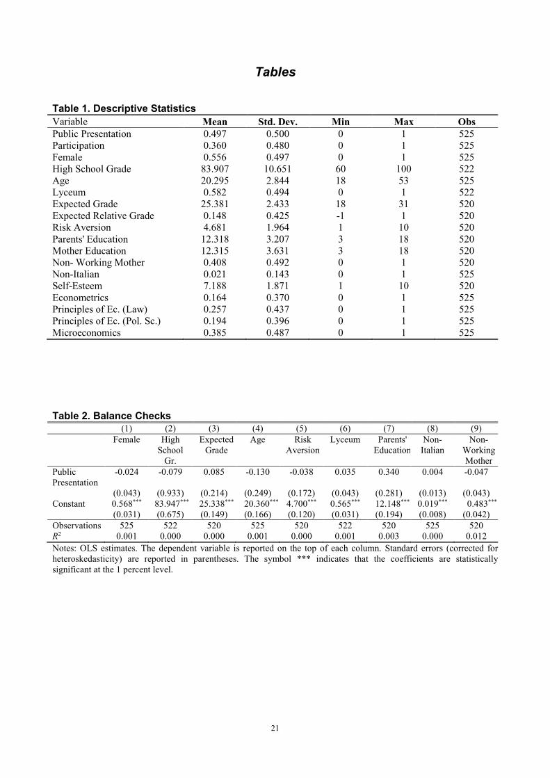
Risk Aversion is a self-reported measure of risk aversion, on a scale from 1 (full availability to take

risks) to 10 (no willingness to take risks); the mean of Risk Aversion is 4.7. Self-Esteem is based on the

answer from 1 to 10 to the question “How satisfied are of yourself?”. The mean value for this variable is 7.2.

As regards family background, on average parents of sample students have acquired 12.3 years of

education. The average number of years of education of mothers is very similar (12.3), but about 41% of

them are not employed (while only 6% of fathers are not employed).

Finally, in most of our regressions we use dummy courses: 38% of our sample students come from

Microeconomics, 26% from Principles of Economics (Degree in Law), 19% from Principles of Economics

(Degree in Political Sciences), 16% from Econometrics.

3.2. Balance Checks Preliminarily, we check if the randomization has been successful in creating comparable treatment and

control groups along a number of observable characteristics.

In Table 2 we regress a number of pre-determined characteristics – in turn – on our treatment

variable Public Presentation. Therefore, in these regressions the coefficient on Public Presentation indicates

if a given characteristic is different in the treatment group with respect to the control group (whose mean is

indicated by the constant). For example, in column (1) we show that 56.8% of students in the control group

are females, while females are 2.4 percentage points less in the treatment group. The difference is far from

statistical significance.

In all the columns – considering, respectively, Female, High School Grade, Expected Grade, Age,

Risk Aversion, Lyceum, Parents’ Education, Non-Italian, Non-Working Mother– we fail to reject the null

hypothesis that there are no significant differences between treatment and control groups.7

We have also run the same regressions controlling for course dummies (since randomization

occurred at the course level) and we find very similar results (not reported).

Table 2 here

4. The Empirical Analysis: Gender and Public Presentation

In this Section we carry out an econometric analysis to investigate if being assigned to the public

presentation leads students to participate less to the proposed task. More importantly, we analyze if the

willingness to do a public presentation depends on gender.

We estimate several specifications of the following simple model: 7 No statistically significant differences are found also for Mother Education, Father Education, Self-Esteem and Expected Relative Grade (results not reported to avoid to clutter the Table).

9

[1]

iCiiiiiii uWXFemale*sentationPublic_PreFemalesentationPublic_PreionParticipat +++++++= φββββββ 543210

where the vector Xi are individual pre-determined characteristics (Age, High School Grade, Lyceum, etc.)

and Wi is a set of variables measuring psychological traits (self-confidence, risk aversion, self-esteem), φc are

courses fixed effects and ui is an error term.

In this setting, β1 is the difference for males in the propensity to give a public presentation with

respect to a face-to-face presentation, while β3 gives us the difference between females and males in the

propensity to give a public presentation (with respect to a face-to-face presentation).

It is worthwhile to notice that an alternative way to organize the experiment would have been to ask

the whole sample of students to give a public presentation (rewarded with a bonus) and verify if males and

females reacted differently. However, in that setting if gender differences in observable or unobservable

factors drive their propensity to participate (for example, it could be that women have higher abilities or are

less eager to obtain a higher grade at the exams), these factors could mix up with a differential aversion to

public speaking and make the gender difference in participation misleading. If factors affecting the decision

to participate are differentiated by gender, we could erroneously end up either by interpreting these

differences as a gender gap in public speaking propensity or fail to find any gender gap. For instance, let us

suppose that women are less interested in the grade they will get at the exam, then in this alternative

experimental setting their lower participation in the public speaking task might depend on this factor instead

of being related to their aversion to the task itself. On the other hand, if they are more interested in obtaining

the bonus, this may compensate their tendency to shy away from public speaking situations leading to no

gender difference in effective behavior. In contrast, randomly assigning students to two different

experimental conditions (Public Presentation or Presentation to the Instructor)8, as we did in our experiment,

allows us to take a sort of “difference-in-differences” and obtain an unbiased estimate of public speaking

aversion, as long as the gender differences in observable and unobservable factors affect similarly the two

types of presentations.

In Table 3 we estimate several specifications of a Linear Probability Model for the probability of

students to participate to the proposed task (homework plus presentation), taking into account the assigned

treatment condition (public or face-to-face presentation). In all the regressions, standard errors (corrected for

heteroskedasticity) are reported in parentheses.

Initially, we show separate estimates by gender: in column (1) we focus only on women, while in

column (2) we consider only men. The main findings of our experiment can be shown in these two columns.

We find that women participate on average 43.3% if assigned to the face-to-face presentation, whereas their

rate of participation reduces drastically to 24.6%, that is, 18.7 percentage points less, if assigned to the public

presentation. The difference is highly statistically significant (t-stat=–3.43). In sharp contrast, men tend to

8 A similar design is used by Ariely et al. (2009) who to investigate the impact of audience on performance run an experiment in which participants were assigned to two different treatments, one in which participants worked on a given task without being observed by anyone and another in which the task was performed in front of an audience.

10

participate less to the face-to-face presentation (38.6%) but there is no difference in their propensity to

participate if they are assigned to the public presentation (37.8%).

In column (3) we estimate on the whole sample of men and women and use an interaction term

between Female and Public Presentation. We confirm that women tend to participate more than men if

assigned to face-to-face presentation (4.7 p.p. more, but the difference is not statistically significant); on the

other hand, they are 17.9 p.p. less likely than men to participate if assigned to the public presentation (t-

stat=–2.13).

In column (4) we control for course dummies, leaving Microeconomics as the reference category.9

We find qualitatively the same results discussed above: women are less inclined to speak in front of a large

public than men (–17.8 p.p.).

Since the propensity to participate could as well depend on student’s academic ability and in our

sample men and women tend to differ in terms of abilities, in column (5) we run the same regression of

column (4) but we control for High School Grade, an important measure of ability (see, among others, De

Paola and Scoppa, 2011).10 We find that 10 additional points of High School Grade (corresponding to about

1 SD) increase the propensity to participate of 8 p.p. (t-stat=4.13). More importantly, the difference between

men and women in the propensity to give a public presentation is almost unchanged (16.8 p.p.; t-stat=–2.11).

Table 3 here

It is useful to graphically show the propensity to speak in public in relation to the High School Grade

for men and women, showing for each quartile of High School Grade the propensity to give a public

presentation (Figure 1). As expected, the propensity to speak in public increases when abilities are higher, for

both men and women. The most striking evidence is that at low levels of abilities, women do not intent to

speak in public at all, while men in the bottom part of the ability distribution show a quite high propensity.

On the other hand, we find a considerable difference also when we look at high skilled individuals, with high

ability women being much less inclined to public speaking compared to their male counterparts.

Figure 1 here

In Table 4, we investigate if the gender difference in the propensity to present publicly is driven by

some additional individual characteristics or by some psychological traits. In column (1), in addition to the

High School Grade, we control for the type of High School attended (Lyceum)11 and for Age. We find that

9 Students attending the Econometrics course participate much more (+21 p.p.), while students enrolled in Law and Political Sciences participate much less (about –16 and –21 p.p., respectively). 10 The gap between males and females in public speaking could be explained in principle if men had higher abilities. Quite the contrary, in terms of High School Grade women show an average value of 85.6, while the average for men is 81.8. The difference of 3.86 is highly statistically significant (t-stat=4.20). 11 In the Italian educational system, the Lyceum (Scientific or Classical Lyceum) offers an academic education, aimed to prepare for University, while technical and professional schools prepare for jobs.

11

students who attended a Lyceum tend to participate much more (+11.6 p.p.), while age – once controlling for

course dummies – does not affect the propensity to participate.12 In column (2) we control in addition for

Parents’ Education, Non-Working Mother and Non-Italian. We find that neither the education of parents nor

the mother’s employment condition produce effects on our dependent variable, while students with an

immigrant background are much less willing to make the presentation (–18.4 p.p.).

In principle, some psychological traits, such as the degree of self-confidence, risk aversion and self-

esteem, that tend to be different between men and women (see, for example, Croson and Gneezy, 2009;

Bertrand, 2011), could drive our main results. Therefore, preliminarily, we verify if any gender differences

emerge along these traits. We find, consistently with the literature, that women – compared to men – are

more risk averse (+0.27, t-stat=1.60), expect to obtain lower grades (–0.43; t-stat=–2.03) and lower relative

grades (–0.11; t-stat=–3.09) and tend to have lower levels of self-esteem (–0.51; t-stat=–3.14).

To take into account these aspects in our analysis, starting from column (3) of Table 4, we

additionally control for the Expected Grade at the exam and for the Expected Relative Grade. These are

measures of both ability and self-confidence. The Expected Grade has a strong positive effect on the

propensity to participate, while the Expected Relative Grade has a positive but weakly significant effect (p-

value=0.12). However, the interaction term Female*(Public Presentation) is almost the same (–14.5

percentage points).

In column (4) we control, in addition, for the degree of Risk Aversion. We find a negative although

not significant effect of this variable on the propensity to participate, but again the coefficient on our

interaction term remains similar (–15 p.p., t-stat=–1.92).

Finally, in column (5) we control for a measure of Self-Esteem. This variable seems to have no effect

on the probability to participate and does not affect our coefficient of interest.

We find very similar results if – instead of a Linear Probability Model – we estimate a Probit model

(results not reported).

Table 4 here

As a further check, in Table 5 we report estimation results for regressions in which we interact each

covariate with the dummy Public Presentation to verify if the gender difference in public presentation is

driven by other gender specific variables. In column (1) we consider the basic set of controls (High School

Grade, Age, Lyceum, Parents’ Education, Non-Working Mother, Non-Italian) and their interaction with

Public Presentation. We find that the coefficient of our interest, Female*Public Presentation, is not affected

(–17.1 p.p.). In column (2) we extend the set of controls in order to include our measures of psychological

traits (Expected Grade, Expected Relative Grade, Risk Aversion and Self-Esteem) and the interaction terms

between these variables and Public Presentation to see which of them affects individual willingness to give a

public presentation. We find that none of these variables is particularly relevant in determining the choice to

12 In contrast, Age has a positive and significant impact when we do not control for course dummies.

12

present in front of a large public. On the other hand, being a female continues to negatively affect public

speaking propensity (–17 p.p., t-stat=–2.02).

The same results hold true when we estimate separate models for female and male students. In

columns (3) and (4) are reported, separately, estimation results for the model including the basic controls,

while in columns (5) and (6) we includes the full set of covariates. In these specifications we find that

females are less likely to participate when assigned to the Public Presentation treatment compared to when

they are required to present in front of the instructor. No statistically significant difference is instead found

for males. The difference between female’s and male’s reaction to the Public Presentation treatment –

calculated comparing the point estimates coming from two different models (column 3 vs. 4 and column 5

vs. 6) – is statistically significant (p-value 0.072 and 0.061, respectively).13

All in all, our estimates show that women are much more averse to public speaking than males and

controlling for individual characteristics does not change this gap. The gender difference remains stable also

when we take into account a number of psychological traits that tend to differ between men and women.

Table 5 here

5. Aversion to Public Speaking and Mothers’ Working Conditions

Women’s aversion to public speaking might depend on gender norms, which, as shown by a large literature,

shape women’s behavior in many domains, such as labor market participation, age at marriage, fertility etc.

(Fernández and Fogli, 2009; Burda et al., 2013; Corrigall and Konrad, 2007; Cunningham et al., 2005;

Fortin, 2005; Stickney and Konrad, 2007; Vella, 1994). Parents transmit gender attitudes to their children

and those gender attitudes, in turn, affect decisions in several economic and social spheres. Studies

investigating the intergenerational transmission of gender role attitudes within the family emphasize the

importance of the mother/daughter intergenerational mechanism and show that having a working mother

leads to more egalitarian gender role attitudes (Fan and Marini, 2000; Fernández et al., 2004; Farré and

Vella, 2013; Berrington et al., 2008; Kawaguchi and Miyazaki, 2009; Johnston et al., 2014; McGinn et al.,

2015; Olivetti et al., 2018).

In this Section, exploiting the availability of information on the labor market conditions of mothers,

we investigate its effects on our measure of public speaking aversion.14 At this aim, we split the sample

according to mothers’ employment condition (employed and not employed) and in Table 6 we report

estimation results separately for female and male students (including the full set of our controls). As shown

in column (1) and (2), controlling for parents’ education, we find that women with mothers who are out of

the labor market tend to be more averse to public speaking (-27.1 p.p.) compared to those whose mothers are

13 Obtained implementing the suest command in STATA. 14 A similar exercise cannot be conducted for fathers given that the vast majority of them is employed.

13

employed (-9.9). The difference is statistically significant at 10 percent level (p-value: 0.094). On the other

hand, no statistically significant differences are instead found for males.

Very similar results are found when we estimate a more parsimonious regression including only

some basic controls, such as High School Grade, Age, Non-Italian and Parents’ Education (results not

reported).

Table 6 here In order to understand whether our results are driven by the fact that unemployed mothers are

typically characterized by a lower education (the correlation between Non-Working Mother and Mother’s

Education is -0.34, (p-value 0.00), we have split our sample in three groups: the first includes students whose

mothers have attained at most lower secondary education the second those with mothers who have acquired

at most a high school degree, and finally students whose mothers have got a tertiary education degree. In

Table 7 we report estimates for only females (columns 1-3) and only males (columns 4-6) in specifications

that include the full set of controls, a dummy variable for Non-Working Mother and the interaction term Non-

Working Mother*Public Presentation. We do not find any evidence of heterogeneity according to the

educational attainment of mothers.

All in all, the estimates reported in this Section show that the employment status of mothers is important

to enhance their daughters’ propensity to engage in public speaking, while the educational background does

not seem to plays any relevant role.

Table 7 here

6. Males’ and Females’ Performance in the Oral Presentation

Following the rules of the experiment, we randomly selected – among students accepting to participate to the

proposed task – 75 students for the oral presentation of their homework, 39 were required to present their

work to the instructor and 36 to the whole class. Among selected students, no one refused to do the

presentation or was absent.

To measure their ability to present clearly and discuss their work in the two different situations, each

instructor has evaluated, at the end of each presentation, student’s performance in terms of clarity and

effectiveness.15

We use these subjective evaluations to try to understand whether the gender difference in the

propensity to speak in public are related to differences in the ability to face this type of context. In Table 8

we use instructors’ subjective performance evaluations as a dependent variable and investigate whether there

is any gender difference in face-to-face presentations or in presentations in front of a large audience.

On the whole, we find that females do not perform worse than males. If anything, females tend to

perform a little better than males both in public presentations (col. 1) and in face-to-face presentations (col.

15 To avoid consequences from possible differential reactions to feedbacks, evaluations were not communicated to students.

14

2). But these differences are not statistically significant (t-stat=1.15 and t-stat=1.12, respectively). No

statistically significant differences emerge also when we run our regressions on the whole sample and

include among regressors the dummy variable Public Presentation and the interaction term Female*Public

Presentation (col. 3, 4 and 5 with different sets of control variables). Females tend to perform better in face-

to-face presentation (+0.468) and also in public presentation (+0.416=0.468-0.052), but these differences are

not statistically significant (notice however that our sample in this case is only 75 obs.).

Admittedly, the evidence we find is only suggestive since participants in both types of presentations

are a self-selected sub-sample. This implies that our results might be due to the fact that we only consider

those females that when assigned to the public speaking presentation have agreed to do so, probably because

they are aware of their ability to successfully deal with such type of circumstances. Furthermore, the

subjective evaluations might be biased because instructors were aware of the aims of the experiment.

Therefore, the results of this Section should be taken with caution.

Table 8 here

7. Survey Evidence on Reactivity to Incentives and Time for Preparation

Individual propensity to deal with the stress implied by public speaking (and the effort provided in order to

be effective in this task) is likely to depend on the rewards deriving from it.

The evidence we have shown in previous Sections refers to a situation in which individuals face

given incentives and a certain amount of time to prepare for the presentation. Then, from our experimental

framework it is not possible to infer how participants would react to stronger or weaker incentives or to

different amounts of time. It could be, for instance, that the gender gap vanishes as incentives are increased

or, on the contrary, that it remains stable also with very high stakes in place. In addition, the time available to

prepare the public speech could be relevant for individual decisions and females might only need a larger

amount of time in order to feel sufficiently confident to speak in front of a large audience.

In order to investigate these aspects in our experiment, it would have been necessary to introduce

many different treatment conditions and then involve a much higher number of students to have sufficiently

large subsamples in each condition. Furthermore, such an experimental framework would have raised some

relevant ethical problems as students with identical characteristics and engaged with the same task would

have been given very different opportunities and rewards. To avoid these problems, in our experiment

students were all given the same reward and the same amount of time to prepare.

Then, in order to better understand how individual aversion to public speaking is affected by

incentives and time availability, we have conducted an on-line Survey among university students not

15

involved in the experiment.16 The decision to propose the Survey to a different group of students was aimed

at avoiding the influence of the assignment treatment on their answers.17

In the Survey, we presented students with a situation very similar to that faced by students involved

in the experiment (see Appendix B). Then, we firstly asked them which kind of presentation they would have

chosen if they had the possibility to do so. Out of 207 respondents, 61% have expressed a preference for the

presentation face-to-face with the instructor (51% among males and 69% among females), 26% were

indifferent (34% among males and 20% among females) and only 13% of students (15% among males and

11% among females) declared to prefer the public presentation.

Based on this question we build the variable Public Speaking Aversion, equal to +1 if a student

prefers a face-to-face presentation, equal to 0 if s/he is indifferent and equal to –1 if s/he prefers a public

presentation. Our aim is to investigate if when students are free to choose their preferences reflect their

choices in the experiment.

In Table 9 we use Public Speaking Aversion as a dependent variable and verify if women are more

averse than men to public speaking. In column (1), without controls, we show that the aversion for women is

0.226 higher than for men (t-stat=2.09). This corresponds to about 0.31 SD of the dependent variable.

Starting from column (2) we control for some individual characteristics. In column (2) we include

among regressors Age and in column (3) we also add High School Grade. We find that female aversion to

public speaking with respect to males is around 0.25 and remains statistically significant. This holds true also

controlling for Lyceum and for nationality (columns 4 and 5, respectively).18

Given the ordinal nature of our dependent variable (averse/indifferent/inclined to public speaking)

we also estimate an Ordered Probit Model and we find very similar results (not reported).

Table 9 here

In our Survey we asked students a number of other questions on their preferences for the type of

presentation by varying the number of points that they could gain through the public presentation with

respect to the face-to-face presentation.

We began by asking students if the public and face-to-face presentation were rewarded 1 point each,

would they be indifferent between the two or would they prefer one or the other. Then, for those answering

that they would prefer a face-to-face presentation, we progressively asked questions increasing the reward

for public presentation to 1.5, 2, 3, 4 (and leaving constant at 1 the reward for the face-to-face presentation).

We build a variable MRS or Marginal Rate of Substitution (the amount of the reward that the individual

16 We wrote an email to students who attended our courses in the previous academic year (2017-2018) asking them to answer to a survey we were conducting for research purposes. About 500 students were contacted with a response rate of about 40%. 17 We have also conducted a similar Survey with students involved in the experiment and we find results that are in line with those presented in this Section (see Appendix C). 18 We have some missing information on the type of High School and the number of observations is reduced in the last specifications.

16

requires to switch from the face-to-face presentation to the public speaking presentation), which takes the

value of 1 if s/he is indifferent, the value of 1.5 if s/he switches to public presentation when the reward is 1.5,

and so on. We impute MRS equal to 5 if the student never wants to switch to the public presentation.

On the other hand, we impute MRS=0.66 (=1/1.5) if s/he prefer the public presentation at our initial

question and switches to the face-to-face presentation when obtaining 1.5; we impute MRS=0.5 if the

switching to the face-to-face presentation occurs when offering 2 points, and so on.

On average, MRS is equal to 2.09, that is, students are willing to give a public presentation for a

reward double with respect to the face-to-face presentation. MRS is 2.41 for females and 1.68 for males.

In Table 10 we use Marginal Rate of Substitution as a dependent variable running the same

regressions of Table 9. We show that females’ Marginal Rate of Substitution is significantly higher, of about

0.7-0.8 points with respect to males, and this difference does not change when we control for Age, High

School Grade, Lyceum and nationality. Notice that the uncovered difference corresponds to 0.50 SD of the

dependent variable.19

Interestingly, these results, even if based on survey questions, are consistent with those found when

using measures of public speaking aversion based on the incentivized experiment. This is relevant not only to

assess the robustness of gender difference in public speaking aversion to the use of different types of public

speaking aversion measures, but also to understand which is the best way to reliably capture this type of

attitude. Consistently with results found by Dohmen et al. (2011) for risk aversion, our results suggest that

survey measures, although far from perfect, can be in some circumstances a useful way to elicit public

speaking aversion.

Table 10 here

An important issue to analyze is whether the gender gap in public presentation tends to close when

the incentives are increased. To investigate this aspect, we have built some sort of supply curves for males

and females in which we report, on the vertical axis, the reward offered for public presentation and, on the

horizontal axis, the percentage of men and women accepting to make the public presentation for each reward

level.20

Figure 2 here

Women’s and men’s reactions to incentives are reported in Figure 2 (respectively, solid and dashed

lines). From the graph, it is clear that women demand a higher reward for speaking in public; more

importantly, the gender gap does not close as incentives increase.

Finally, following some studies that have found that women suffer more than men under time

pressure (see, for example, De Paola and Gioia, 2016), we investigate if for women the aversion to public

19 These questions were asked also to students involved in the experiment. As shown in Appendix C of the paper, also for those students we find that the Marginal Rate of Substitution is higher for females. 20 On the horizontal axis we use the percentage rather than the simple number of individuals since the number of male and female respondents were different (respectively, 91 and 116).

17

speaking is related to time availability, that is, if they feel more confident and more prone to speak in public

when they have more time to prepare for the presentation.

To this aim, in our Survey we asked students if they were willing to make a public presentation (with

a reward of 1 point) if they had 5 days of time to prepare. Subsequently, we asked the same question but

changing from 5 to 15 the days available to prepare (in the previous questions of the Survey students were

told that they had 10 days of time).

As expected, results show that students are on average less likely to give a public presentation if they

have 5 days of time to prepare it than if they have 15 days (53% and 86% of them answered affirmatively in

the two alternative situations).

In Table 11, in the first three columns we examine the students’ willingness to deliver the

presentation if they had 5 days and in columns 4-6 we examine their willingness if they had 15 days. Our aim

is to verify if the gender gap widens or closes as time availability increases.

If having more time would allow women to overcome their aversion to public presentation, we

should find a higher gender gap when time availability is set at 5 days compared to when it is set at 15 days.

In contrast to our expectations, we find that with 5 days of time men and women do not differ in their

willingness to give the public presentation – the coefficient on Female is negative but far from statistical

significance. On the other hand, men turn out to be more reactive than women when time availability

increases to 15 days: 91% of them are willing to give the public presentation, while this percentage becomes

83% for women. So, men have a greater propensity of about 8 percentage points if time for preparation is

longer. Therefore, our results suggest that it is not time pressure that discourages women to do a public

presentation.

Table 11 here

8. Concluding Remarks A number of psychological traits – such as risk aversion, willingness to compete, aversion to feedbacks –

have been recently identified as particularly relevant in contributing to explain gender differences in

occupations, wages and careers.

Public speaking is generally thought to be relevant for career prospects and leadership positions. The

ability to present information publicly, clearly and eloquently gives an important competitive advantage in a

variety of job settings. While giving individuals valuable opportunities, speaking to a public is also a

possible source of anxiety and embarrassment. Little is known on factors affecting the willingness to face

public speaking situations or the ability to deal with the stress deriving from this type of exposure to

judgment and to be effective in public speech. Men and women could differ in the anxiety generated by

public speaking and, therefore, be differently averse to public speaking. This in turn could cause gender

differences in career prospects and access to top positions.

We contribute to the literature on this topic by running a field experiment allowing us to analyze

whether, in an incentivized setting, men and women show differences in their willingness to speak in public.

18

The experiment involved more than 500 undergraduate students who could gain two points to add to the final

grade of their exam by presenting orally the solutions of a problem set. Students were randomly assigned to

present in front of a large audience (a class of about 100 students or more) or, in alternative, only to the

instructor.

We find very relevant differences among men and women in their willingness to present in public.

While women are more willing to present face-to-face, they are considerably less likely to give a public

presentation. We are able to show that this tendency does not depend on differences in individual abilities or

in other psychological traits as risk aversion, self-confidence and self-esteem.

We also find that women with employed mothers are more prone to public speaking compared to

women whose mothers are out of the labor market. This is in line with a growing literature showing that

having a working mother leads to more egalitarian gender role attitudes.

Moreover, using data from an online Survey, we show that giving higher incentives for public

presentation does not allow to close the gender gap in public speaking aversion. Even when the gains

deriving from public speaking are quite high, women are much less likely than men to engage in this type of

activity. Finally, we also find that women do not seem to benefit from increasing the amount of time

available to prepare for the task.

These findings suggest that women’s tendency to shy away from public speaking situations is

difficult to change, as it is probably the result of deeply embedded social norms.

This kind of aversion – together with other psychological traits such as risk aversion and

unwillingness to compete – could be a relevant factor in explaining the gender differences in access to high-

level positions and career prospects and, then, it is important to understand both how to design work and

educational environments in order to not harm certain categories of the population and how to help women to

overcome their aversion to public speaking.

Future research can greatly contribute to this objective, by trying to better understand whether

individual aversion to public speaking responds to some specific situational aspects, such as the topic of the

speech, the size and gender composition (and other characteristics) of the audience and by investigating

whether and how this type of attitude is susceptible to changes over time, also in relation to specific policy

interventions. For instance, it would be very interesting to assess the effectiveness of public speaking training

or to understand if exposure to public speaking, allowing individuals to learn how to deal with the emotions

deriving from it, helps at overcoming aversion.

References Azmat G., Calsamiglia C., Iriberri N. (2016), Gender Differences in Response to Big Stakes, Journal of the

European Economic Association, 14(6), 1372–1400. Ariely D., Gneezy U., Loewenstein G., Mazar N. (2009), Large Stakes and Big Mistakes, The Review of

Economic Studies, 76(2), 451–469. Atkinson, A. B., Casarico, A., Voitchovsky, S. (2018). Top incomes and the gender divide. The Journal of

Economic Inequality, 16(2), 225-256. Ayres, J., Schliesman, T. S. (2002). Paradoxical Intention: An Alternative for the Reduction of

19

Communication Apprehension? Communication Research Reports, 19(1), 38-45. Azmat, G. Petrongolo, B. (2014). Gender and the labor market: What have we learned from field and lab

experiments? Labour Economics, 30, 32-40. Babcock, L., Recalde, M. P., Vesterlund, L., Weingart, L. (2017). Gender differences in accepting and

receiving requests for tasks with low promotability. American Economic Review, 107(3), 714-47. Bar-Haim, E., Chauvel, L., Gornick, J., Hartung, A. (2018). The persistence of the gender earnings gap:

Cohort trends and the role of education in twelve countries. Inequality Matters-LIS newsletter, Issue No. 6.

Behnke R., Sawyer, C. (2000). Anticipatory anxiety patterns for male and female public speakers. Communication Education, 49(2), 187-195.

Berrington, A., Hu, Y., Smith, P. W. Sturgis, P. (2008). A graphical chain model for reciprocal relationships between women’s gender role attitudes and labour force participation. Journal of the Royal Statistical Society: Series A (Statistics in Society), 171(1), 89-108.

Bertrand, M. (2018). Coase Lecture–The Glass Ceiling. Economica, 85(338), 205-231. Bertrand, M. (2011), “New Perspectives on Gender”, Handbook of Labor Economics, 4b, Amsterdam:

North-Holland. Blau, F. D., Kahn, L. M. (2017). The gender wage gap: Extent, trends, and explanations. Journal of

Economic Literature, 55(3), 789-865. Bodie, G. D. (2010). A racing heart, rattling knees, and ruminative thoughts: Defining, explaining, and

treating public speaking anxiety. Communication education, 59(1), 70-105. Burda, M., Hamermesh, D. S., Weil, P. (2013). Total work and gender: facts and possible explanations.

Journal of Population Economics, 26(1), 239-261. Buser, T., Niederle, M., Oosterbeek, H. (2014). Gender, competitiveness, and career choices. The Quarterly

Journal of Economics, 129(3), 1409-1447. Carter, A. J., Croft, A., Lukas, D., Sandstrom, G. M. (2018). Women’s visibility in academic seminars:

Women ask fewer questions than men. PloS one, 13(9), e0202743. Castillo, G. A. (2010). “Assessing the effectiveness of public speaking instruction on students' cognitive

learning, skill development, and communication apprehension”. The University of Texas-Pan American.

Corrigall, E. A., Konrad, A. M. (2007). Gender role attitudes and careers: A longitudinal study. Sex Roles, 56(11-12), 847-855.

Croson, R., Gneezy U. (2009). Gender Differences in Preferences. Journal of Economic Literature, 47 (2), 448-74.

Cunningham, M., Beutel, A.M., Barber, J.S., Thornton, A. (2005). Reciprocal relationships between attitudes about gender and social contexts during young adulthood. Social Science Research, 34,862–892.

Daly, J. A., Caughlin, J. P., Stafford, L. (1997). Correlates and consequences of social communicative anxiety. In J. A. Daly, J. C. McCroskey, J. Ayres, T. Hopf, and D. M. Ayres (Eds.), Avoiding communication: Shyness, reticence, and communication apprehension (pp. 21-74). Cresskill, NJ: Hampton Press.

De Paola, M., Gioia, F. (2016). Who performs better under time pressure? Results from a field experiment. Journal of Economic Psychology, 53, 37-53.

De Paola, M., Scoppa, V. (2011). Frequency of examinations and student achievement in a randomized experiment. Economics of Education Review, 30(6), 1416-1429.

De Paola, M., Scoppa, V. (2015). Procrastination, academic success and the effectiveness of a remedial program. Journal of Economic Behavior& Organization, 115, 217-236.

Dohmen, T., Falk, A., Huffman, D., Sunde, U., Schupp, J., Wagner, G. (2011). Individual Risk Attitudes: Measurement, Determinants, and Behavioral Consequences. Journal of the European Economic Association, Vol. 9. No. 3. pp. 522–550.

Eddy, S. L., Brownell, S. E., Wenderoth, M. P. (2014). Gender gaps in achievement and participation in multiple introductory biology classrooms. CBE—Life Sciences Education, 13(3), 478-492.

Fallows, S., Steven, C. (2000). Building employability skills into the higher education curriculum: a university-wide initiative. Education+ training, 42(2), 75-83.

Fan, Pi-Ling, Mooney Marini M. (2000). Influences on gender-role attitudes during the transition to adulthood. Social Science Research, 29.2 258-283.

Farré, L., Vella, F. (2013). The intergenerational transmission of gender role attitudes and its implications for female labour force participation. Economica, 80(318), 219-247.

20

Fernandez, R., & Fogli, A. (2009). Culture: An empirical investigation of beliefs, work, and fertility. American economic journal: Macroeconomics, 1(1), 146-77.

Fernández, R., Fogli, A., Olivetti, C. (2004). Mothers and sons: Preference formation and female labor force dynamics. Quarterly Journal of Economics, 119(4), 1249-1299.

Fortin, N. M. (2005). Gender role attitudes and the labour-market outcomes of women across OECD countries. Oxford Review of Economic Policy, 21(3), 416-438.

Hart Research Associates (2015). Falling short? College learning and career success. Association of American Colleges and Universities.

Hinsley, A., Sutherland, W. J., Johnston, A. (2017). Men ask more questions than women at a scientific conference. PloS one, 12(10), e0185534.

Holmes, J. (1992). Women's talk in public contexts. Discourse & Society, 3(2), 131-150. Johnston, D. W., Schurer, S., Shields, M. A. (2014). Maternal gender role attitudes, human capital

investment, and labour supply of sons and daughters. Oxford Economic Papers, 66(3), 631-659. Kamas, L., Preston, A. (2012). The importance of being confident; gender, career choice, and willingness to

compete. Journal of Economic Behavior & Organization, 83(1), 82-97. Karpowitz, C. F., Mendelberg, T., Shaker, L. (2012). Gender inequality in deliberative participation.

American Political Science Review, 106(3), 533-547. Kawaguchi, D., Miyazaki, J. (2009). Working mothers and sons’ preferences regarding female labor supply:

direct evidence from stated preferences. Journal of Population Economics, 22(1), 115-130. Kirschbaum, C., Pirke, K-M., Hellhammer D.H. (1993). The ‘Trier Social Stress Test’–a tool for

investigating psychobiological stress responses in a laboratory setting. Neuropsychobiology, 28 (1-2), 76-81.

Lustig, M. W., Andersen, P. A. (1990). Generalizing about communication apprehension and avoidance: Multiple replications and meta-analyses. Journal of Social Behavior & Personality, 5(4), 309.

Marinho, A. C. F., de Medeiros, A. M., Gama, A. C. C., Teixeira, L. C. (2017). Fear of public speaking: Perception of college students and correlates. Journal of Voice, 31(1), 127e.7- 127e.11.

McCroskey, J. C. (1997). Self-report measurement. In J. A. Daly, J. C. McCroskey, J. Ayres, T. Hopf, and D. M. Ayres (Eds.), Avoiding communication: Shyness, reticence, and communication apprehension (pp. 191-216). Cresskill, NJ: Hampton Press.

McGinn, K. L., Mayra, R. C. Lingo, E. L. (2015). Mums the word! Cross-national Effects of Maternal Employment on Gender Inequalities at Work and at Home. Tech. rep., Harvard Business School Working Paper No. 15-094.

Niederle, M. (2015). “Gender” in: Handbook of Experimental Economics. Princeton University Press, pp. 481–563.

Niederle, M. Vesterlund, L. (2007). Do Women Shy Away from Competition? Do men Compete Too Much? Quarterly Journal of Economics, 122 (3), 1067-1101.

Olivetti, C., Patacchini, E. Zenou, Y. (2018). Mothers, Peers and Gender Identity," Boston College Working Papers in Economics 904, Boston College Department of Economics.

Robinson, T. E. (1997). Communication apprehension and the basic public speaking course: A national survey of in-class treatment techniques. Communication Education, 46(3), 188-197.

Schmidt, S. J., Davenport, J. R. (2017). Who asks questions at astronomy meetings? New Astron., 1, 1-2. Scoppa, V., Stranges, M. (2019). Cultural Values and Decision to Work of Immigrant Women in Italy.

Labour, 33(1), 101-123. Shurchkov, O. (2012). Under pressure: gender differences in output quality and quantity under competition

and time constraints. Journal of the European Economic Association, 10(5), 1189-1213. Stickney, Lisa T., Konrad A. M. (2007). Gender-role attitudes and earnings: A multinational study of

married women and men. Sex Roles, pp. 801-811. Vella, F. (1994). Gender roles and human capital investment: the relationship between traditional attitudes

and female labour market performance. Economica, 61, 191–211 Zabava Ford, W. S., Wolvin A.D. (1993). The differential impact of a basic communication course on

perceived communication competencies in class, work, and social contexts. Communication Education, (42)1, 215-223.

21

Tables Table 1. Descriptive Statistics Variable Mean Std. Dev. Min Max Obs Public Presentation 0.497 0.500 0 1 525 Participation 0.360 0.480 0 1 525 Female 0.556 0.497 0 1 525 High School Grade 83.907 10.651 60 100 522 Age 20.295 2.844 18 53 525 Lyceum 0.582 0.494 0 1 522 Expected Grade 25.381 2.433 18 31 520 Expected Relative Grade 0.148 0.425 -1 1 520 Risk Aversion 4.681 1.964 1 10 520 Parents' Education 12.318 3.207 3 18 520 Mother Education 12.315 3.631 3 18 520 Non- Working Mother 0.408 0.492 0 1 520 Non-Italian 0.021 0.143 0 1 525 Self-Esteem 7.188 1.871 1 10 520 Econometrics 0.164 0.370 0 1 525 Principles of Ec. (Law) 0.257 0.437 0 1 525 Principles of Ec. (Pol. Sc.) 0.194 0.396 0 1 525 Microeconomics 0.385 0.487 0 1 525

Table 2. Balance Checks (1) (2) (3) (4) (5) (6) (7) (8) (9) Female High

School Gr.

Expected Grade

Age Risk Aversion

Lyceum Parents' Education

Non-Italian

Non- Working Mother

Public Presentation

-0.024 -0.079 0.085 -0.130 -0.038 0.035 0.340 0.004 -0.047

(0.043) (0.933) (0.214) (0.249) (0.172) (0.043) (0.281) (0.013) (0.043) Constant 0.568*** 83.947*** 25.338*** 20.360*** 4.700*** 0.565*** 12.148*** 0.019*** 0.483*** (0.031) (0.675) (0.149) (0.166) (0.120) (0.031) (0.194) (0.008) (0.042) Observations 525 522 520 525 520 522 520 525 520 R2 0.001 0.000 0.000 0.001 0.000 0.001 0.003 0.000 0.012 Notes: OLS estimates. The dependent variable is reported on the top of each column. Standard errors (corrected for heteroskedasticity) are reported in parentheses. The symbol *** indicates that the coefficients are statistically significant at the 1 percent level.

22

23

Table 3. Public Presentation and Gender. OLS Estimates (1)

Females (2)

Males (3) All

(4) All

(5) All

Public Presentation -0.187*** -0.008 -0.008 -0.004 -0.008 (0.054) (0.064) (0.064) (0.061) (0.061) Female 0.047 0.062 0.032 (0.061) (0.061) (0.061) Female*(Public Presentation) -0.179** -0.178** -0.168** (0.084) (0.081) (0.079) Econometrics 0.210*** 0.220*** (0.063) (0.063) Principles of Ec. (Law) -0.158*** -0.182*** (0.054) (0.053) Principles of Ec. (Pol.Sc.) -0.210*** -0.161*** (0.052) (0.053) High School Grade 0.008*** (0.002) Constant 0.433*** 0.386*** 0.386*** 0.422*** -0.240 (0.041) (0.046) (0.046) (0.050) (0.166) Observations 292 233 525 525 522 R2 0.039 0.000 0.023 0.109 0.141 Notes: OLS estimates (Linear Probability Model). The dependent variable is Participation. Standard errors (corrected for heteroskedasticity) are reported in parentheses. The symbols ***, **, * indicate that the coefficients are statistically significant at the 1, 5 and 10 percent level, respectively. Table 4. Public Presentation and Gender: Controlling for Self-confidence, Risk Aversion, Self-Esteem. OLS Estimates (1) (2) (3) (4) (5) Public Presentation -0.013 -0.021 -0.026 -0.024 -0.025 (0.061) (0.062) (0.060) (0.060) (0.061) Female 0.033 0.025 0.043 0.049 0.048 (0.061) (0.062) (0.061) (0.062) (0.062) Female*(Public Presentation) -0.166** -0.151* -0.145* -0.150* -0.150* (0.079) (0.080) (0.079) (0.079) (0.079) High School Grade 0.008*** 0.008*** 0.007*** 0.007*** 0.007*** (0.002) (0.002) (0.002) (0.002) (0.002) Age 0.000 0.001 -0.000 -0.001 -0.001 (0.005) (0.005) (0.005) (0.005) (0.005) Lyceum 0.116*** 0.124*** 0.117*** 0.118*** 0.118*** (0.040) (0.041) (0.041) (0.041) (0.041) Parents' Education 0.001 -0.002 -0.002 -0.002 (0.007) (0.007) (0.007) (0.007) Non-Working Mother 0.032 0.036 0.036 0.036 (0.042) (0.041) (0.041) (0.041) Non-Italian -0.184* -0.172* -0.146 -0.148 (0.098) (0.100) (0.099) (0.102) Expected Grade 0.022** 0.022** 0.022** (0.009) (0.009) (0.009) Expected Relative Grade 0.090 0.085 0.085 (0.058) (0.058) (0.059) Risk Aversion -0.013 -0.013 (0.010) (0.010) Self-Esteem -0.001 (0.010) Courses dummies YES YES YES YES YES Observations 522 518 518 518 518 R2 0.155 0.159 0.185 0.187 0.187 Notes: OLS estimates (Linear Probability Model). The dependent variable is Participation. Standard errors (corrected for heteroskedasticity) are reported in parentheses. The symbols ***, **, * indicate that the coefficients are statistically significant at the 1, 5 and 10 percent level, respectively.

24

Table 5. Public Presentation and Gender: Using All Set of Interactions. OLS Estimates (1) (2) (3) (4) (5) (6) All All Females Males Females Males Public Presentation -0.073 0.255 -0.168*** -0.029 -0.171*** -0.027 (0.467) (0.584) (0.050) (0.061) (0.050) (0.060) Female 0.034 0.062 (0.063) (0.065) Female*(Public Presentation) -0.171** -0.170** (0.082) (0.084) High School Grade 0.006** 0.005* 0.008*** 0.007** 0.007*** 0.007** (0.003) (0.003) (0.002) (0.003) (0.003) (0.003) Age 0.003 -0.002 0.004 -0.009 0.003 -0.011 (0.011) (0.010) (0.005) (0.020) (0.005) (0.018) Lyceum 0.084 0.064 0.150*** 0.065 0.129** 0.088 (0.062) (0.062) (0.053) (0.064) (0.054) (0.061) Parents' Education 0.008 0.002 -0.001 0.006 -0.003 -0.000 (0.011) (0.011) (0.008) (0.011) (0.008) (0.011) Non- Working Mother 0.102* 0.107* 0.111** -0.050 0.123** -0.063 (0.062) (0.061) (0.054) (0.068) (0.053) (0.067) Non-Italian -0.282 -0.129 -0.332*** -0.014 -0.297*** 0.025 (0.205) (0.195) (0.105) (0.154) (0.083) (0.166) Self-Predicted Grade 0.034** 0.023* 0.028* (0.015) (0.012) (0.016) Predicted Relative Grade 0.048 0.039 0.096 (0.085) (0.077) (0.091) Risk-Aversion -0.013 -0.002 -0.028* (0.010) (0.013) (0.016) Self-Esteem -0.001 -0.004 0.009 (0.010) (0.014) (0.016) High School Gr.*(Public Pres.) 0.003 0.004 (0.004) (0.004) Age*(Public Pres.) -0.003 0.001 (0.013) (0.013) Lyceum*(Public Pres.) 0.092 0.111 (0.081) (0.081) Parents Ed.*(Public Pres.) -0.013 -0.008 (0.014) (0.014) Non-Working Mother*(Public Pres)

-0.141* -0.143*

(0.083) (0.083) Non-Italian*(Public Pres.) 0.186 0.010 (0.217) (0.213) Expected Gr.*(Public Pres.) -0.021 (0.018) Exp. Rel. Grade*(Public Pres.) 0.064 (0.117) Risk Aversion*(Public Pres.) 0.003 (0.021) Self-Esteem*(Public Pres.) -0.007 (0.022) Courses Dummies YES YES YES YES YES YES Observations 518 518 288 230 288 230 R2 0.167 0.197 0.228 0.149 0.245 0.206 Notes: OLS estimates (Linear Probability Model). The dependent variable is Participation. Standard errors (corrected for heteroskedasticity) are reported in parentheses. The symbols ***, **, * indicate that the coefficients are statistically significant at the 1, 5 and 10 percent level, respectively.

25

Table 6. Heterogeneous Effects of Mothers’ Occupational Condition on Public Speaking Aversion. OLS Estimates Females Males Non-Working

Mother Working Mother Non-Working Mother Working Mother

(1) (2) (3) (4) Public Presentation -0.271*** -0.099 -0.049 -0.017 (0.088) (0.063) (0.090) (0.083) High School Grade 0.009* 0.006* 0.006 0.008* (0.005) (0.003) (0.005) (0.005) Age -0.004 0.003 -0.029 0.009 (0.039) (0.010) (0.027) (0.036) Lyceum 0.115 0.164** 0.091 0.045 (0.094) (0.072) (0.099) (0.090) Non-Italian -0.307 -0.286 0.125 -0.143 (0.360) (0.244) (0.316) (0.303) Parents' Education 0.009 -0.011 0.001 -0.002 (0.015) (0.011) (0.016) (0.016) Self-Predicted Grade 0.024 0.021 0.039 0.008 (0.024) (0.016) (0.024) (0.025) Predicted Relative Grade

0.001 0.079 0.215 0.083

(0.148) (0.095) (0.131) (0.118) Risk-Aversion 0.012 -0.012 -0.061** -0.009 (0.022) (0.017) (0.027) (0.022) Self-Esteem 0.005 -0.007 0.016 0.001 (0.028) (0.018) (0.026) (0.026) Courses Dummies YES YES YES YES Observations 115 173 96 134 R-squared 0.256 0.239 0.302 0.199 Notes: OLS estimates (Linear Probability Model). The dependent variable is Participation. Standard errors (corrected for heteroskedasticity) are reported in parentheses. The symbols ***, **, * indicate that the coefficients are statistically significant at the 1, 5 and 10 percent level, respectively.

Table 7. Heterogeneous Effects of Mother’s Educational Level on Public Speaking Aversion. OLS Estimates (1) (2) (3) (4) (5) (6) Females Males Mother:

<High School

Mother: High School

Mother: College

Mother: <High School

Mother: High School

Mother: College

Public Presentation -0.083 -0.116 -0.121 -0.306 0.028 -0.060 (0.158) (0.102) (0.180) (0.251) (0.125) (0.195) Non-Working Mother 0.108 0.234* 0.199 -0.420** 0.048 -0.157 (0.141) (0.118) (0.298) (0.207) (0.134) (0.234) Non-Working Mother *Public Presentation

-0.098 -0.302* 0.231 0.324 -0.059

(0.201) (0.168) (0.450) (0.304) (0.192) Observations 97 111 53 57 114 42 R2 0.278 0.299 0.244 0.358 0.190 0.435 Notes: OLS estimates (Linear Probability Model). The dependent variable is Participation. In all specifications we include the basic set of controls (High School Grade, Age, Lyceum, Parents’ Education, Nationality and course dummies). Standard errors (corrected for heteroskedasticity) are reported in parentheses. The symbols ***, **, * indicate that the coefficients are statistically significant at the 1, 5 and 10 percent level, respectively.

26

Table 8. Performance of Men and Women in the Oral Presentation. OLS Estimates (1)

Public pres. (2)

Face-to-face pres.

(3) All

(4) All

(5) All

Female 0.416 0.468 0.468 0.435 0.420 (0.364) (0.417) (0.417) (0.388) (0.391) Public Presentation 0.348 0.320 0.390 (0.442) (0.390) (0.359) Female*(Public Presentation) -0.052 -0.054 -0.222 (0.553) (0.503) (0.501) High School Grade 0.027** (0.013) Expected Grade 0.053 (0.048) Lyceum -0.377 (0.273) Constant 3.289*** 2.941*** 2.941*** 3.414*** -0.017 (0.261) (0.357) (0.357) (0.314) (1.424) Courses dummies YES YES YES YES YES Observations 36 39 75 75 75 R2 0.037 0.036 0.050 0.227 0.316 Notes: OLS estimates. The dependent variable is Evaluation of the Presentation. Standard errors (corrected for heteroskedasticity) are reported in parentheses. The symbols ***, **, * indicate that the coefficients are statistically significant at the 1, 5 and 10 percent level, respectively. Table 9. Aversion to Public Speaking from Students’ Survey. OLS Estimates (1) (2) (3) (4) (5) Female 0.226** 0.239** 0.253** 0.286** 0.300*** (0.100) (0.102) (0.104) (0.114) (0.113) Age -0.002 -0.002 0.000 0.006 (0.018) (0.021) (0.022) (0.022) High School Grade -0.004 -0.004 -0.004 (0.005) (0.005) (0.005) Lyceum -0.059 -0.074 (0.111) (0.110) Non-Italian -0.810*** (0.267) Constant 0.352*** 0.367 0.743 0.690 0.531 (0.077) (0.433) (0.641) (0.674) (0.668) Observations 207 202 199 174 174 R2 0.025 0.028 0.031 0.042 0.069 Notes: OLS estimates. The dependent variable is Aversion to Public Speaking. Standard errors (corrected for heteroskedasticity) are reported in parentheses. The symbols ***, **, * indicate that the coefficients are statistically significant at the 1, 5 and 10 percent level, respectively.

27

Table 10. Marginal Rate of Substitution. OLS estimates (1) (2) (3) (4) (5) Female 0.725*** 0.773*** 0.867*** 0.849*** 0.872*** (0.183) (0.183) (0.189) (0.198) (0.198) Age -0.011 -0.022 -0.032 -0.022 (0.036) (0.040) (0.042) (0.042) High School Grade -0.025** -0.019* -0.018* (0.009) (0.010) (0.010) Lyceum -0.057 -0.082 (0.201) (0.201) Non-Italian -1.310*** (0.325) Constant 1.683*** 1.861** 4.184*** 3.934*** 3.674*** (0.114) (0.831) (1.333) (1.394) (1.380) Observations 206 201 198 173 173 R2 0.066 0.078 0.111 0.109 0.130 Notes: OLS estimates. The dependent variable is Marginal Rate of Substitution. Standard errors (corrected for heteroskedasticity) are reported in parentheses. The symbols ***, **, * indicate that the coefficients are statistically significant at the 1, 5 and 10 percent level, respectively. Table 11. Availability of Time and Public Presentation. OLS estimates (1) (2) (3) (4) (5) (6) Presentation

in 5 days Presentation

in 15 days

Female -0.013 -0.036 -0.059 -0.085* -0.108** -0.108** (0.070) (0.072) (0.073) (0.046) (0.046) (0.047) Age -0.017 -0.011 -0.001 -0.004 (0.013) (0.014) (0.009) (0.010) High School Grade 0.004 -0.001 (0.003) (0.002) Constant 0.538*** 0.942*** 0.508 0.912*** 0.964*** 1.122*** (0.053) (0.306) (0.479) (0.030) (0.206) (0.309) Observations 207 202 199 207 202 199 R2 0.000 0.008 0.013 0.015 0.025 0.028 Notes: OLS estimates. In columns 1-3 the dependent variable is Public Presentation in 5 days; in columns 4-6 the dependent variable Public Presentation in 15 days. Standard errors (corrected for heteroskedasticity) are reported in parentheses. The symbols ***, **, * indicate that the coefficients are statistically significant at the 1, 5 and 10 percent level, respectively.

28

Figures

Figure 1. Propensity to Speak in Public for Males and Females and High School Grade (in quartiles)

Figure 2. Males’ and Females’ “Supply Curves” for Public Presentation

0.1

.2.3

.4.5

Parti

cipa

tion

in P

ublic

Spe

akin

g

1 2 3 4Quartiles of High School Grade

Females Males

01

23

45

0 .2 .4 .6 .8 1Fraction of male or female students

Females' MRS FemalesMales' MRS Males

29

Appendix A. Instructions to Students

Students attending this course have the possibility to gain a bonus of two points to be added to the final grade, by doing a homework consisting in solving a set of questions/exercises and orally presenting the solutions. The questions involving both theoretical reasoning and numerical and graphical analysis will be published on the course webpage and students will have two weeks of time to solve them and submit them to the instructor. The type of the presentation depends on whether the student has been randomly allocated to one of the following groups: 1. "Presentation to the Instructor": students included in this group will have to present some exercises to

the instructor during office hours; 2. "Presentation to the Class": students included in this group will have to present some exercises in front

of the whole class (plus the instructor). The list of students included in each group will be published on the course web page. By submitting the solutions, students agree to do the oral presentation of some of the exercises/questions included in the homework. The presentation is planned seven days after the submission of solutions to the problem set. One third of students in each group who have submitted the homework will be randomly drawn for the presentation.

Students submitting their work will obtain two extra points to add to the final grade exam, regardless of the fact that they have been drawn to do the presentation.

Students submitting their work and randomly drawn for the oral presentation who will be absent the day of the presentation or who will refuse to present will be penalized with a reduction of two points of the final mark obtained at the exam.

Presentations will be organized in two subsequent days. The first day, at the end of the teaching class, will be communicated the names of the students randomly drawn for the presentation in front to the instructor. These students will be required to join the instructor in her/his office and present to her/him the work. The following day, at the beginning of the class, the list of randomly drawn students to present to the class will be communicated. These students will be invited, following a random order, to present some of the questions/exercises (following the order in which the problem set was organized).

Participation to the homework is not compulsory, students are completely free to join it (according to the rules written above) or to not participate.

All participant and non-participant students will take the exam in the standard way at the end of the course, with questions and exercises covering the whole course program evaluated with a maximum score of 30 points and a minimum passing score of 18.

Examples of problems students had to solve as homework Microeconomics and Principles of Economics

1) Give a definition of indifference curve; draw the indifference curve. What does the slope of this curve represents? What does it represent from an economic point of view?

2) What are the effects of introducing a consumption tax? What determines the side of the market on which the tax burden weighs most?

3) Luisa spends part of her income buying books. Her utility function is u (x, y) = xy2 where x indicates the quantity of books and y represents consumption in all other goods. Knowing that the monthly income of Luisa is equal to 900 euros, the price of x is 10 euros and the price of y is 5 euros: i) Write Luisa's budget constraint and represent it graphically; indicate the intercepts and the slope. ii) Calculate the marginal utility of books and goods y and indicate the Marginal Substitution Rate. iii) Calculate the optimal consumer choice.

4) Explain what is and what causes the Keynesian multiplier

30

5) Consider an economy that produces and consumes bread and automobiles. In the following table are data for two different years.

Year

2000 2010

Good Quantity Price Quantity Price

Automobiles 100 50

120 60 Bread 500 10 400 20

a) Using the year 2000 as the base year, compute the following statistics for each year:

− Nominal GDP, − Real GDP, − The GDP deflator

b) How much have prices risen between 2000 and 2010? Econometrics

1) Suppose you have estimated the following model: ii COMPUTERY 10ˆˆˆ ββ += where Y represents the

performance of students at school (Test score) and COMPUTER is a dummy equal to 1 if the student has a computer (and zero otherwise). 1̂β is positive and significantly different from zero. There is no information on the BACKGROUND variable (which summarizes the socio-economic characteristics of the family). Considering the omitted variable problem, is 1̂β an unbiased estimator? Is it consistent? Show formally under what conditions it is biased and the sign of the bias.

2) Discuss possible sources of biases of Standard Errors estimations and potential remedies.

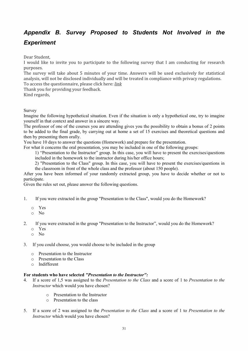
31

Appendix B. Survey Proposed to Students Not Involved in the Experiment

Dear Student, I would like to invite you to participate to the following survey that I am conducting for research purposes. The survey will take about 5 minutes of your time. Answers will be used exclusively for statistical analysis, will not be disclosed individually and will be treated in compliance with privacy regulations. To access the questionnaire, please click here: link Thank you for providing your feedback. Kind regards, Survey Imagine the following hypothetical situation. Even if the situation is only a hypothetical one, try to imagine yourself in that context and answer in a sincere way. The professor of one of the courses you are attending gives you the possibility to obtain a bonus of 2 points to be added to the final grade, by carrying out at home a set of 15 exercises and theoretical questions and then by presenting them orally. You have 10 days to answer the questions (Homework) and prepare for the presentation. For what it concerns the oral presentation, you may be included in one of the following groups:

1) “Presentation to the Instructor” group. In this case, you will have to present the exercises/questions included in the homework to the instructor during his/her office hours; 2) "Presentation to the Class" group. In this case, you will have to present the exercises/questions in the classroom in front of the whole class and the professor (about 150 people).

After you have been informed of your randomly extracted group, you have to decide whether or not to participate. Given the rules set out, please answer the following questions.

1. If you were extracted in the group "Presentation to the Class", would you do the Homework?

o Yes o No

2. If you were extracted in the group "Presentation to the Instructor”, would you do the Homework?

o Yes o No

3. If you could choose, you would choose to be included in the group

o Presentation to the Instructor o Presentation to the Class o Indifferent

For students who have selected "Presentation to the Instructor": 4. If a score of 1,5 was assigned to the Presentation to the Class and a score of 1 to Presentation to the

Instructor which would you have chosen?

o Presentation to the Instructor o Presentation to the class

5. If a score of 2 was assigned to the Presentation to the Class and a score of 1 to Presentation to the

Instructor which would you have chosen?

32

o Presentation to the Instructor o Presentation to the Class

6. If a score of 3 was assigned to the Presentation to the Class and a score of 1 to Presentation to the

Instructor which would you have chosen?

o Presentation to the Instructor o Presentation to the Class

7. If a score of 4 had been assigned to the Presentation to the Class and a score of 1 to Presentation to the

Instructor which would you have chosen?

o Presentation to the Instructor o Presentation to the Class

For students who have selected "Presentation to the Class":

8. If a score of 1.5 was assigned to the Presentation to the Instructor and a score of 1 to the Presentation to the Class which would you have chosen?

o Presentation to the Instructor o Presentation to the Class

9. If a score of 2 was assigned to the Presentation to the Instructor and a score of 1 to the Presentation to

the Class which would you have chosen?

o Presentation to the Instructor o Presentation to the Class

10. If a score of 3 was assigned to the Presentation to the Instructor and a score of 1 to the Presentation to

the Class which would you have chosen?

o Presentation to the Instructor o Presentation to the Class

11. If a score of 4 was assigned to the Presentation to the Instructor and a score of 1 to the Presentation to

the Class which would you have chosen?

o Presentation to the Instructor o Presentation to the Class

Consider now the preparation time for the Homework (with a bonus of 2 points for participation). 12. If you have been included in the group "Presentation to the Class" and the time you have available is 15

days (instead of 10 days), would you decide to do the Homework?

o Yes o No

13. If you have been included in the group "Presentation to the Class " and the time you have available is 5

days (instead of 10 days), would you decide to do the Homework?

o Yes o No

14. If you have been included in the group "Presentation to the Instructor " and the time you have available

is 15 days (instead of 10 days), would you decide to do the Homework?

33

o Yes o No

15. If you have been included in the group "Presentation to the Instructor" and the time you have available is 5 days (instead of 10 days), would you decide to do the Homework?

o Yes o No

Appendix C. Further Evidence from a Post Experiment Survey

In order to better understand the behavior of students deciding to join our experiment, we have proposed them a post experiment survey. Alike to what done for the survey discussed in Section 7, we asked students to answer to a number of questions on their preferences for the type of presentation by varying the number of points that they could gain through the public presentation with respect to the face-to-face presentation (we asked students questions 3 to 14 reported in Appendix B above). We began by proposing a situation in which the public and face-to-face presentation were rewarded 1 point each and asking if they were indifferent between the two or if they prefer one or the other. Then, for those answering that they prefer a face-to-face presentation, we progressively asked questions increasing the reward for public presentation to 1.5, 2, 3, 4 (and leaving constant at 1 the rewards for the face-to-face presentation). Based on these questions we build the variable MRS in the way described in Section 7. We find that students who were involved in the experiment are willing to give a public presentation for a reward double with respect to the face-to-face presentation (on average, MRS is equal to 1.98). The average value for MRS is 2.14 for females and 1.80 for males. We use MRS as a dependent variable to analyze gender differences. In column (1) we only include among regressors the dummy variable Female, while in the subsequent columns we control for some individual characteristics, such as Age (column 2), High School Grade (column 3), Lyceum (column 4) and nationality (column 5). Findings, reported in Table C1, are consistent with those presented in Section 7. Also for this sample of students we find that females’ MRS is significantly higher, of about 0.3-0.4 points, with respect to males. The magnitude of the coefficient and its statistical significance increase when we add individual characteristics among regressors. Table C1. Marginal Rate of Substitution. OLS estimates (1) (2) (3) (4) (5) Female 0.334* 0.311 0.454** 0.503** 0.494** (0.195) (0.198) (0.204) (0.205) (0.208) Age 0.030 0.011 0.004 0.004 (0.036) (0.040) (0.038) (0.038) High School Grade -0.023** -0.025** -0.025** (0.011) (0.011) (0.011) Lyceum -0.474** -0.469** (0.215) (0.216) Non-Italian -0.436** (0.167) Constant 1.805*** 1.177 3.526** 4.072*** 4.038*** (0.124) (0.734) (1.430) (1.443) (1.453) Observations 160 160 160 160 160 R2 0.012 0.013 0.037 0.065 0.060 Notes: OLS estimates. The dependent variable is Marginal Rate of Substitution. Standard errors (corrected for heteroskedasticity) are reported in parentheses. The symbols ***, **, * indicate that the coefficients are statistically significant at the 1, 5 and 10 percent level, respectively.

34

To investigate whether the gender gap in the willingness to give a public presentation tends to close when incentives increase, we have built two supply curves for males and females respectively, in which on the vertical axis we indicate the reward offered for the public presentation and on the horizontal axis we report the percentage of men and women accepting the offer for each reward. In Figure C1 we plot these curves (solid and dashed lines for women and men, respectively). Also in this case it emerges that women demand a higher reward for speaking in public (although the gender gap appears to be smaller compared to that found in Section 7) and that higher incentives does not allow to close the gap.

Figure C1. Males’ and Females’ “Supply Curves” for Public Presentation

01

23

45

0 .2 .4 .6 .8 1Fraction of male or female students

Females' MRS FemalesMales' MRS Males