distributions and their fourier transforms

Chapter 4

Distributions and Their FourierTransforms

4.1 The Day of Reckoning

We’ve been playing a little fast and loose with the Fourier transform — applying Fourier inversion, appeal-ing to duality, and all that. “Fast and loose” is an understatement if ever there was one, but it’s also truethat we haven’t done anything “wrong”. All of our formulas and all of our applications have been correct,if not fully justified. Nevertheless, we have to come to terms with some fundamental questions. It will takeus some time, but in the end we will have settled on a very wide class of signals with these properties:

• The allowed signals include δ’s, unit steps, ramps, sines, cosines, and all other standard signals thatthe world’s economy depends on.

• The Fourier transform and its inverse are defined for all of these signals.

• Fourier inversion works.

These are the three most important features of the development to come, but we’ll also reestablish someof our specific results and as an added benefit we’ll even finish off differential calculus!

4.1.1 A too simple criterion and an example

It’s not hard to write down an assumption on a function that guarantees the existence of its Fouriertransform and even implies a little more than existence.

• If∫ ∞

−∞|f(t)| dt <∞ then Ff and F−1f exist and are continuous.

Existence follows from

|Ff(s)| =∣∣∣∣∫ ∞

−∞e−2πistf(t) dt

∣∣∣∣

≤∫ ∞

−∞|e−2πist| |f(t)| dt=

∫ ∞

−∞|f(t)| dt <∞ .

138 Chapter 4 Distributions and Their Fourier Transforms

Here we’ve used that the magnitude of the integral is less that the integral of the magnitude.1 There’sactually something to say here, but while it’s not complicated, I’d just as soon defer this and othercomments on “general facts on integrals” to Section 4.3; read it if only lightly — it provides some additionalorientation.

Continuity is the little extra information we get beyond existence. Continuity follows as follows. For anys and s′ we have

|Ff(s)− Ff(s′)| =∣∣∣∣∫ ∞

−∞e−2πistf(t) dt−

∫ ∞

−∞e−2πis′tf(t) dt

∣∣∣∣

=∣∣∣∣∫ ∞

−∞(e−2πist − e−2πis′t)f(t) dt

∣∣∣∣ ≤∫ ∞

−∞|e−2πist − e−2πis′t| |f(t)| dt

As a consequence of∫∞−∞ |f(t)| dt < ∞ we can take the limit as s′ → s inside the integral. If we do that

then |e−2πist − e−2πis′t| → 0, that is,

|Ff(s)−Ff(s′)| → 0 as s′ → s

which says that Ff(s) is continuous. The same argument works to show that F−1f is continuous.2

We haven’t said anything here about Fourier inversion — no such statement appears in the criterion. Let’slook right away at an example.

The very first example we computed, and still an important one, is the Fourier transform of Π. We founddirectly that

FΠ(s) =∫ ∞

−∞e−2πistΠ(t) dt =

∫ 1/2

−1/2e−2πist dt = sinc s .

No problem there, no problem whatsoever. The criterion even applies; Π is in L1(R) since∫ ∞

−∞|Π(t)| dt =

∫ 1/2

−1/21 dt = 1 .

Furthermore, the transform FΠ(s) = sinc s is continuous. That’s worth remarking on: Although the signaljumps (Π has a discontinuity) the Fourier transform does not, just as guaranteed by the preceding result— make this part of your intuition on the Fourier transform vis a vis the signal.

Appealing to the Fourier inversion theorem and what we called duality, we then said

Fsinc(t) =∫ ∞

−∞e−2πist sinc t dt = Π(s) .

Here we have a problem. The sinc function does not satisfy the integrability criterion. It is my sad dutyto inform you that ∫ ∞

−∞| sinc t| dt = ∞ .

I’ll give you two ways of seeing the failure of | sinc t| to be integrable. First, if sinc did satisfy the criterion∫∞−∞ | sinc t| dt < ∞ then its Fourier transform would be continuous. But its Fourier transform, which has

1 Magnitude, not absolute value, because the integral is complex number.

2 So another general fact we’ve used here is that we can take the limit inside the integral. Save yourself for other things andlet some of these “general facts” ride without insisting on complete justifications — they’re everywhere once you let the rigorpolice back on the beat.

4.1 The Day of Reckoning 139

to come out to be Π, is not continuous. Or, if you don’t like that, here’s a direct argument. We canfind infinitely many intervals where | sinπt| ≥ 1/2; this happens when t is between 1/6 and 5/6, and thatrepeats for infinitely many intervals, for example on In = [16 + 2n, 5

6 + 2n], n = 0, 1, 2, . . . , because sinπtis periodic of period 2. The In all have length 2/3. On In we have |t| ≤ 5

6 + 2n, so

1|t| ≥

15/6 + 2n

and ∫

In

| sinπt|π|t|

dt ≥ 12π

15/6 + 2n

∫

In

dt =12π

23

15/6 + 2n

.

Then ∫ ∞

−∞

| sinπt|π|t|

dt ≥∑

n

∫

In

| sinπt|π|t|

dt =13π

∞∑

n=1

15/6 + 2n

= ∞ .

It’s true that | sinc t| = | sinπt/πt| tends to 0 as t→ ±∞ — the 1/t factor makes that happen — but not“fast enough” to make the integral of | sinc t| converge.

This is the most basic example in the theory! It’s not clear that the integral defining the Fourier transformof sinc exists, at least it doesn’t follow from the criterion. Doesn’t this bother you? Isn’t it a littleembarrassing that multibillion dollar industries seem to depend on integrals that don’t converge?

In fact, there isn’t so much of a problem with either Π or sinc. It is true that

∫ ∞

−∞e−2πist sinc s ds =

{1 |t| < 1

2

0 |t| > 12

However showing this — evaluating the improper integral that defines the Fourier transform — requiresspecial arguments and techniques. The sinc function oscillates, as do the real and imaginary parts of thecomplex exponential, and integrating e−2πist sinc s involves enough cancellation for the limit

lima→−∞b→∞

∫ b

ae−2πist sinc s ds

to exist.

Thus Fourier inversion, and duality, can be pushed through in this case. At least almost. You’ll noticethat I didn’t say anything about the points t = ±1/2, where there’s a jump in Π in the time domain. Inthose cases the improper integral does not exist, but with some additional interpretations one might beable to convince a sympathetic friend that

∫ ∞

−∞e−2πi(±1/2)s sinc s ds = 1

2

in the appropriate sense (invoking “principle value integrals” — more on this in a later lecture). At bestthis is post hoc and needs some fast talking.3

The truth is that cancellations that occur in the sinc integral or in its Fourier transform are a very subtleand dicey thing. Such risky encounters are to be avoided. We’d like a more robust, trustworthy theory.

3 One might also then argue that defining Π(±1/2) = 1/2 is the best choice. I don’t want to get into it.


The news so far Here’s a quick summary of the situation. The Fourier transform of f(t) is definedwhen ∫ ∞

−∞|f(t)| dt <∞ .

We allow f to be complex valued in this definition. The collection of all functions on R satisfying thiscondition is denoted by L1(R), the superscript 1 indicating that we integrate |f(t)| to the first power.4

The L1-norm of F is defined by

‖f‖1 =∫ ∞

−∞|f(t)| dt .

Many of the examples we worked with are L1-functions — the rect function, the triangle function, theexponential decay (one or two-sided), Gaussians — so our computations of the Fourier transforms in thosecases were perfectly justifiable (and correct). Note that L1-functions can have discontinuities, as in therect function.

The criterion says that if f ∈ L1(R) then Ff exists. We can also say

|Ff(s)| =∣∣∣∣∫ ∞

−∞e−2πistf(t) dt

∣∣∣∣ ≤∫ ∞

−∞|f(t)| dt = ‖f‖1 .

That is:

• The magnitude of the Fourier transform is bounded by the L1-norm of the function.

This is a handy estimate to be able to write down — we’ll use it shortly. However, to issue a warning:

Fourier transforms of L1(R) functions may themselves not be in L1, like for the sinc function, so wedon’t know without further work what more can be done, if anything.

The conclusion is that L1-integrability of a signal is just too simple a criterion on which to build a reallyhelpful theory. This is a serious issue for us to understand. Its resolution will greatly extend the usefulnessof the methods we have come to rely on.

There are other problems, too. Take, for example, the signal f(t) = cos 2πt. As it stands now, this signaldoes not even have a Fourier transform — does not have a spectrum! — for the integral

∫ ∞

−∞e−2πist cos 2πt dt

does not converge, no way, no how. This is no good.

Before we bury L1(R) as too restrictive for our needs, here’s one more good thing about it. There’s actuallya stronger consequence for Ff than just continuity.

• If∫ ∞

−∞|f(t)| dt <∞ then Ff(s) → 0 as s→ ±∞.

4 And the letter “L” indicating that it’s really the Lebesgue integral that should be employed.

4.1 The Day of Reckoning 141

This is called the Riemann-Lebesgue lemma and it’s more difficult to prove than showing simply that Ffis continuous. I’ll comment on it later; see Section 4.19. One might view the result as saying that Ff(s) isat least trying to be integrable. It’s continuous and it tends to zero as s → ±∞. Unfortunately, the factthat Ff(s) → 0 does not imply that it’s integrable (think of sinc, again).5 If we knew something, or couldinsist on something about the rate at which a signal or its transform tends to zero at ±∞ then perhapswe could push on further.

4.1.2 The path, the way

To repeat, we want our theory to encompass the following three points:

• The allowed signals include δ’s, unit steps, ramps, sines, cosines, and all other standard signals thatthe world’s economy depends on.

• The Fourier transform and its inverse are defined for all of these signals.

• Fourier inversion works.

Fiddling around with L1(R) or substitutes, putting extra conditions on jumps — all have been used. Thepath to success lies elsewhere. It is well marked and firmly established, but it involves a break with theclassical point of view. The outline of how all this is settled goes like this:

1. We single out a collection of functions S for which convergence of the Fourier integrals is assured,for which a function and its Fourier transform are both in S, and for which Fourier inversion works.Furthermore, Parseval’s identity holds:

∫ ∞

−∞|f(x)|2 dx =

∫ ∞

−∞|Ff(s)|2ds .

This much is classical; new ideas with new intentions, yes, but not new objects. Perhaps surprisinglyit’s not so hard to find a suitable collection S, at least if one knows what one is looking for. Butwhat comes next is definitely not “classical”. It had been first anticipated and used effectively in anearly form by O. Heaviside, developed, somewhat, and dismissed, mostly, soon after by less talentedpeople, then cultivated by and often associated with the work of P. Dirac, and finally refined byL. Schwartz.

2. S forms a class of test functions which, in turn, serve to define a larger class of generalized functions ordistributions, called, for this class of test functions the tempered distributions, T . Precisely becauseS was chosen to be the ideal Fourier friendly space of classical signals, the tempered distributionsare likewise well suited for Fourier methods. The collection of tempered distributions includes, forexample, L1 and L2-functions (which can be wildly discontinuous), the sinc function, and complexexponentials (hence periodic functions). But it includes much more, like the delta functions andrelated objects.

3. The Fourier transform and its inverse will be defined so as to operate on these tempered distributions,and they operate to produce distributions of the same type. Thus the inverse Fourier transform canbe applied, and the Fourier inversion theorem holds in this setting.

4. In the case when a tempered distributions “comes from a function” — in a way we’ll make precise— the Fourier transform reduces to the usual definition as an integral, when the integral makessense. However, tempered distributions are more general than functions, so we really will have donesomething new and we won’t have lost anything in the process.

5 For that matter, a function in L1(R) need not tend to zero at ±∞; that’s also discussed in Appendix 1.


Our goal is to hit the relatively few main ideas in the outline above, suppressing the considerable massof details. In practical terms this will enable us to introduce delta functions and the like as tools forcomputation, and to feel a greater measure of confidence in the range of applicability of the formulas.We’re taking this path because it works, it’s very interesting, and it’s easy to compute with. I especiallywant you to believe the last point.

We’ll touch on some other approaches to defining distributions and generalized Fourier transforms, butas far as I’m concerned they are the equivalent of vacuum tube technology. You can do distributions inother ways, and some people really love building things with vacuum tubes, but wouldn’t you rather learnsomething a little more up to date?

4.2 The Right Functions for Fourier Transforms: Rapidly DecreasingFunctions

Mathematics progresses more by making intelligent definitions than by proving theorems. The hardestwork is often in formulating the fundamental concepts in the right way, a way that will then make thedeductions from those definitions (relatively) easy and natural. This can take awhile to sort out, anda subject might be reworked several times as it matures; when new discoveries are made and one seeswhere things end up, there’s a tendency to go back and change the starting point so that the trip becomeseasier. Mathematicians may be more self-conscious about this process, but there are certainly examplesin engineering where close attention to the basic definitions has shaped a field — think of Shannon’s workon Information Theory, for a particularly striking example.

Nevertheless, engineers, in particular, often find this tiresome, wanting to do something and not “just talkabout it”: “Devices don’t have hypotheses”, as one of my colleagues put it. One can also have too muchof a good thing — too many trips back to the starting point to rewrite the rules can make it hard tofollow the game, especially if one has already played by the earlier rules. I’m sympathetic to both of thesecriticisms, and for our present work on the Fourier transform I’ll try to steer a course that makes thedefinitions reasonable and lets us make steady forward progress.

4.2.1 Smoothness and decay

To ask “how fast” Ff(s) might tend to zero, depending on what additional assumptions we might makeabout the function f(x) beyond integrability, will lead to our defining “rapidly decreasing functions”,and this is the key. Integrability is too weak a condition on the signal f , but it does imply that Ff(s) iscontinuous and tends to 0 at ±∞. What we’re going to do is study the relationship between the smoothnessof a function — not just continuity, but how many times it can be differentiated — and the rate at whichits Fourier transform decays at infinity.

We’ll always assume that f(x) is absolutely integrable, and so has a Fourier transform. Let’s suppose,more stringently, that

• xf(x) is integrable, i.e.,∫ ∞

−∞|xf(x)| dx <∞ .

4.2 The Right Functions for Fourier Transforms: Rapidly Decreasing Functions 143

Then xf(x) has a Fourier transform, and so does −2πixf(x) and its Fourier transform is

F(−2πixf(x)) =∫ ∞

−∞(−2πix)e−2πisxf(x) dx

=∫ ∞

−∞

(d

dse−2πisx

)f(x) dx =

d

ds

∫ ∞

−∞e−2πisxf(x) dx

(switching d/ds and the integral is justified by the integrability of |xf(x)|)

=d

ds(Ff)(s)

This says that the Fourier transform Ff(s) is differentiable and that its derivative is F(−2πixf(x)). Whenf(x) is merely integrable we know that Ff(s) is merely continuous, but with the extra assumption on theintegrability of xf(x) we conclude that Ff(s) is actually differentiable. (And its derivative is continuous.Why?)

For one more go-round in this direction, what if x2f(x) is integrable? Then, by the same argument,

F((−2πix)2f(x)) =∫ ∞

−∞(−2πix)2e−2πisxf(x) dx

=∫ ∞

−∞

(d2

ds2e−2πisx

)f(x) dx =

d2

ds2

∫ ∞

−∞e−2πisxf(x) dx =

d2

ds2(Ff)(s) ,

and we see that Ff is twice differentiable. (And its second derivative is continuous.)

Clearly we can proceed like this, and as a somewhat imprecise headline we might then announce:

• Faster decay of f(x) at infinity leads to a greater smoothness of the Fourier transform.

Now let’s take this in another direction, with an assumption on the smoothness of the signal. Supposef(x) is differentiable, that its derivative is integrable, and that f(x) → 0 as x → ±∞. I’ve thrown in allthe assumptions I need to justify the following calculation:

Ff(s) =∫ ∞


=[f(x)

e−2πisx

−2πis

]x=∞

x=−∞−∫ ∞

−∞

e−2πisx

−2πisf ′(x) dx

(integration by parts with u = f(x), dv = e−2πisxdx)

=1

2πis

∫ ∞

−∞e−2πisxf ′(x) dx (using f(x) → 0 as x→ ±∞)

=1

2πis(Ff ′)(s)

We then have|Ff(s)| = 1

2πs|(Ff ′)(s)| ≤ 1

2πs‖f ′‖1 .

The last inequality follows from the result: “The Fourier transform is bounded by the L1-norm of thefunction”. This says that Ff(s) tends to 0 at ±∞ like 1/s. (Remember that ‖f ′‖1 is some fixed numberhere, independent of s.) Earlier we commented (without proof) that if f is integrable then Ff tends to 0at ±∞, but here with the stronger assumptions we get a stronger conclusion, that Ff tends to zero at acertain rate.


Let’s go one step further in this direction. Suppose f(x) is twice differentiable, that its first and secondderivatives are integrable, and that f(x) and f ′(x) tend to 0 as x→ ±∞. The same argument gives

Ff(s) =∫ ∞


=1

2πis

∫ ∞

−∞e−2πisxf ′(x) dx (picking up on where we were before)

=1

2πis

([f ′(x)

e−2πisx

−2πis

]x=∞

x=−∞−∫ ∞

−∞

e−2πisx

−2πisf ′′(x) dx

)

(integration by parts with u = f ′(x), dv = e−2πisxdx)

=1

(2πis)2

∫ ∞

−∞e−2πisxf ′′(x) dx (using f ′(x) → 0 as x→ ±∞)

=1

(2πis)2(Ff ′′)(s)

Thus|Ff(s)| ≤ 1

|2πs|2‖f ′′‖1

and we see that Ff(s) tends to 0 like 1/s2.

The headline:

• Greater smoothness of f(x), plus integrability, leads to faster decay of the Fourier transform at ∞.

Remark on the derivative formula for the Fourier transform The astute reader will have noticedthat in the course of our work we rederived the derivative formula

Ff ′(s) = 2πisFf(s)

which we’ve used before, but here we needed the assumption that f(x) → 0, which we didn’t mentionbefore. What’s up? With the technology we have available to us now, the derivation we gave, above, isthe correct derivation. That is, it proceeds via integration by parts, and requires some assumption likef(x) → 0 as x → ±∞. In homework (and in the solutions to the homework) you may have given aderivation that used duality. That only works if Fourier inversion is known to hold. This was OK when therigor police were off duty, but not now, on this day of reckoning. Later, when we develop a generalizationof the Fourier transform, we’ll see that the derivative formula again holds without what seem now to beextraneous conditions.

We could go on as we did above, comparing the consequences of higher differentiability, integrability,smoothness and decay, bouncing back and forth between the function and its Fourier transform. The greatinsight in making use of these observations is that the simplest and most useful way to coordinate all thesephenomena is to allow for arbitrarily great smoothness and arbitrarily fast decay. We would like to haveboth phenomena in play. Here is the crucial definition.

Rapidly decreasing functions

A function f(x) is said to be rapidly decreasing at ±∞ if1. It is infinitely differentiable.


2. For all positive integers m and n,∣∣∣∣xm dn

dxnf(x)

∣∣∣∣→ 0 as x→ ±∞

In words, any positive power of x times any order derivative of f tends to zero at infinity.

Note that m and n are independent in this definition. That is, we insist that, say, the 5th power of x timesthe 17th derivative of f(x) tends to zero, and that the 100th power of x times the first derivative of f(x)tends to zero; and whatever you want.

Are there any such functions? Any infinitely differentiable function that is identically zero outside somefinite interval is one example, and I’ll even write down a formula for one of these later. Another example isf(x) = e−x2

. You may already be familiar with the phrase “the exponential grows faster than any powerof x”, and likewise with the phrase “e−x2

decays faster than any power of x.”6 In fact, any derivative ofe−x2

decays faster than any power of x as x → ±∞, as you can check with L’Hopital’s rule, for example.We can express this exactly as in the definition:

∣∣∣∣xm dn

dxne−x2

∣∣∣∣→ 0 as x→ ±∞

There are plenty of other rapidly decreasing functions. We also remark that if f(x) is rapidly decreasingthen it is in L1(R) and in L2(R); check that yourself.

An alternative definition An equivalent definition for a function to be rapidly decreasing is to assumethat for any positive integers m and n there is a constant Cmn such that

∣∣∣∣xm dn

dxnf(x)

∣∣∣∣ ≤ Cmn as x→ ±∞ .

In words, the mth power of x times the nth derivative of f remains bounded for all m and n, though theconstant will depend on which m and n we take. This condition implies the “tends to zero” condition,above. Convince yourself of that, the key being that m and n are arbitrary and independent. We’ll usethis second, equivalent condition often, and it’s a matter of taste which one takes as a definition.

Let us now praise famous men It was the French mathematician Laurent Schwartz who singled outthis relatively simple condition to use in the service of the Fourier transform. In his honor the set of rapidlydecreasing functions is usually denoted by S (a script S) and called the Schwartz class of functions.

Let’s start to see why this was such a good idea.

1. The Fourier transform of a rapidly decreasing function is rapidly decreasing. Let f(x) bea function in S. We want to show that Ff(s) is also in S. The condition involves derivatives of Ff , sowhat comes in is the derivative formula for the Fourier transform and the version of that formula for higherderivatives. As we’ve already seen

2πisFf(s) =(F d

dxf)(s) .

6 I used e−x2as an example instead of e−x (for which the statement is true as x → ∞) because I wanted to include x → ±∞,

and I used e−x2instead of e−|x| because I wanted the example to be smooth. e−|x| has a corner at x = 0.


As we also noted,d

dsFf(s) = F(−2πixf(x)) .

Because f(x) is rapidly decreasing, the higher order versions of these formulas are valid; the derivationsrequire either integration by parts or differentiating under the integral sign, both of which are justified.That is,

(2πis)nFf(s) =(F dn

dxnf)(s)

dn

dsnFf(s) = F

((−2πix)nf(x)

).

(We follow the convention that the zeroth order derivative leaves the function alone.)

Combining these formulas one can show, inductively, that for all nonnegative integers m and n,

F(

dn

dxn

((−2πix)mf(x)

))= (2πis)n dm

dsmFf(s) .

Note how m and n enter in the two sides of the equation.

We use this last identity together with the estimate for the Fourier transform in terms of the L1-norm ofthe function. Namely,

|s|n∣∣∣∣

dm

dsmFf(s)

∣∣∣∣ = (2π)m−n

∣∣∣∣F(

dn

dxn(xmf(x))

)∣∣∣∣ ≤ (2π)m−n

∥∥∥∥dn

dxn(xmf(x))

∥∥∥∥1

The L1-norm on the right hand side is finite because f is rapidly decreasing. Since the right hand sidedepends on m and n, we have shown that there is a constant Cmn with

∣∣∣∣sndm

dsmFf(s)

∣∣∣∣ ≤ Cmn .

This implies that Ff is rapidly decreasing. Done.

2. Fourier inversion works on S. We first establish the inversion theorem for a timelimited functionin S. Suppose that f(t) is smooth and for some T is identically zero for |t| ≥ T/2, rather than just tendingto zero at ±∞. In this case we can periodize f(t) to get a smooth, periodic function of period T . Expandthe periodic function as a converging Fourier series. Then for −T/2 ≤ t ≤ T/2,

f(t) =∞∑

n=−∞cne

2πint/T

=∞∑

n=−∞e2πint/T

(1T

∫ T/2

−T/2e−2πinx/T f(x) dx

)

=∞∑

n=−∞e2πint/T

(1T

∫ ∞

−∞e−2πinx/T f(x) dx

)=

∞∑

n=−∞e2πint/TFf

(n

T

) 1T.

Our intention is to let T get larger and larger. What we see is a Riemann sum for the integral∫ ∞

−∞e2πistFf(s) ds = F−1Ff(t) ,


and the Riemann sum converges to the integral because of the smoothness of f . (I have not slippedanything past you here, but I don’t want to quote the precise results that make all this legitimate.) Thus

f(t) = F−1Ff(t) ,

and the Fourier inversion theorem is established for timelimited functions in S.

When f is not timelimited we use “windowing”. The idea is to cut f(t) off smoothly.7 The interestingthing in the present context — for theoretical rather than practical use — is to make the window so smooththat the “windowed” function is still in S. Some of the details are in Section 4.20, but here’s the setup.

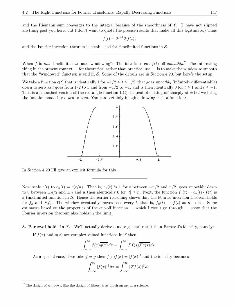
We take a function c(t) that is identically 1 for −1/2 ≤ t ≤ 1/2, that goes smoothly (infinitely differentiable)down to zero as t goes from 1/2 to 1 and from −1/2 to −1, and is then identically 0 for t ≥ 1 and t ≤ −1.This is a smoothed version of the rectangle function Π(t); instead of cutting off sharply at ±1/2 we bringthe function smoothly down to zero. You can certainly imagine drawing such a function:

In Section 4.20 I’ll give an explicit formula for this.

Now scale c(t) to cn(t) = c(t/n). That is, cn(t) is 1 for t between −n/2 and n/2, goes smoothly downto 0 between ±n/2 and ±n and is then identically 0 for |t| ≥ n. Next, the function fn(t) = cn(t) · f(t) isa timelimited function in S. Hence the earlier reasoning shows that the Fourier inversion theorem holdsfor fn and Ffn. The window eventually moves past every t, that is, fn(t) → f(t) as n → ∞. Someestimates based on the properties of the cut-off function — which I won’t go through — show that theFourier inversion theorem also holds in the limit.

3. Parseval holds in S. We’ll actually derive a more general result than Parseval’s identity, namely:

If f(x) and g(x) are complex valued functions in S then∫ ∞

−∞f(x)g(x)dx =

∫ ∞

−∞Ff(s)Fg(s)ds .

As a special case, if we take f = g then f(x)f(x) = |f(x)|2 and the identity becomes∫ ∞

−∞|f(x)|2 dx =

∫ ∞

−∞|Ff(s)|2ds .

7 The design of windows, like the design of filters, is as much an art as a science.


To get the first result we’ll use the fact that we can recover g from its Fourier transform via the inversiontheorem. That is,

g(x) =∫ ∞

−∞Fg(s)e2πisx ds .

The complex conjugate of the integral is the integral of the complex conjugate, hence

g(x) =∫ ∞

−∞Fg(s)e−2πisx ds .

The derivation is straightforward, using one of our favorite tricks of interchanging the order of integration:∫ ∞

−∞f(x)g(x)dx =

∫ ∞

−∞f(x)

(∫ ∞

−∞Fg(s)e−2πisx ds

)dx

=∫ ∞

−∞

∫ ∞

−∞f(x)Fg(s)e−2πisx ds ds

=∫ ∞

−∞

∫ ∞

−∞f(x)Fg(s)e−2πisx dx dx

=∫ ∞

−∞

(∫ ∞

−∞f(x)e−2πisx dx

)Fg(s)ds

=∫ ∞

−∞Ff(s)Fg(s)ds

All of this works perfectly — the initial appeal to the Fourier inversion theorem, switching the order ofintegration — if f and g are rapidly decreasing.

4.3 A Very Little on Integrals

This section on integrals, more of a mid-chapter appendix, is not a short course on integration. It’s hereto provide a little, but only a little, background explanation for some of the statements made earlier. Thestar of this section is you. Here you go.

Integrals are first defined for positive functions In the general approach to integration (of real-valued functions) you first set out to define the integral for nonnegative functions. Why? Because howevergeneral a theory you’re constructing, an integral is going to be some kind of limit of sums and you’ll want toknow when that kind of limit exists. If you work with positive (or at least nonnegative) functions then theissues for limits will be about how big the function gets, or about how big the sets are where the functionis or isn’t big. You feel better able to analyze accumulations than to control conspiratorial cancellations.

So you first define your integral for functions f(x) with f(x) ≥ 0. This works fine. However, you knowfull well that your definition won’t be too useful if you can’t extend it to functions which are both positiveand negative. Here’s how you do this. For any function f(x) you let f+(x) be its positive part :

f+(x) = max{f(x), 0}

Likewise, you letf−(x) = max{−f(x), 0}

be its negative part.8 (Tricky: the “negative part” as you’ve defined it is actually a positive function; taking−f(x) flips over the places where f(x) is negative to be positive. You like that kind of thing.) Then

f = f+ − f−

8 A different use of the notation f− than we had before, but we’ll never use this one again.

4.3 A Very Little on Integrals 149

while|f | = f+ + f− .

You now say that f is integrable if both f+ and f− are integrable — a condition which makes sense sincef+ and f− are both nonnegative functions — and by definition you set

Zf =

Zf+ −

Zf− .

(For complex-valued functions you apply this to the real and imaginary parts.) You follow this approachfor integrating functions on a finite interval or on the whole real line. Moreover, according to this definition|f | is integrable if f is because then

Z|f | =

Z(f+ + f−) =

Zf+ +

Zf−

and f+ and f− are each integrable.9 It’s also true, conversely, that if |f | is integrable then so is f . Youshow this by observing that

f+ ≤ |f | and f− ≤ |f |

and this implies that both f+ and f− are integrable.

• You now know where the implication∫ ∞

−∞|f(t)| dt <∞ ⇒ Ff exists comes from.

You get an easy inequality out of this development:∣∣∣Zf∣∣∣ ≤

Z|f | .

In words, “the absolute value of the integral is at most the integral of the absolute value”. And sure that’strue, because

∫f may involve cancellations of the positive and negative values of f while

∫|f | won’t have

such cancellations. You don’t shirk from a more formal argument:∣∣∣Zf∣∣∣ =

∣∣∣Z

(f+ − f−)∣∣∣ =

∣∣∣Zf+ −

Zf−∣∣∣

≤∣∣∣Zf+∣∣∣+∣∣∣Zf−∣∣∣ =

Zf+ +

Zf− (since f+ and f− are both nonnegative)

=Z

(f+ + f−) =Z|f | .

• You now know where the second inequality in

|Ff(s)−Ff(s′)| =∣∣∣∣∫ ∞

−∞

(e−2πist − e−2πis′ t

)f(t) dt

∣∣∣∣ ≤∫ ∞

−∞

∣∣∣e−2πist − e−2πis′t∣∣∣ |f(t)| dt

comes from; this came up in showing that Ff is continuous.

9 Some authors reserve the term “summable” for the case whenR|f | < ∞, i.e., for when both

Rf+ and

Rf− are finite. They

still defineR

f =R

f+ −R

f− but they allow the possibility that one of the integrals on the right may be ∞, in which caseRf is ∞ or −∞ and they don’t refer to f as summable.


sinc stinks What about the sinc function and trying to make sense of the following equation?

Fsinc(s) =∫ ∞

−∞e−2πist sinc t dt

According to the definitions you just gave, the sinc function is not integrable. In fact, the argument I gaveto show that ∫ ∞

−∞| sinc t| dt = ∞

(the second argument) can be easily modified to show that both∫ ∞

−∞sinc+t dt = ∞ and

∫ ∞

−∞sinc−t dt = ∞ .

So if you wanted to write ∫ ∞

−∞sinc t dt =

∫ ∞

−∞sinc+t dt−

∫ ∞

−∞sinc−t dt

you’d be faced with ∞−∞. Bad. The integral of sinc (and also the integral of F sinc) has to be understoodas a limit,

lima→−∞, b→∞

∫ b

a

e−2πist sinc t dt

Evaluating this is a classic of contour integration and the residue theorem, which you may have seen in aclass on “Functions of a Complex Variable”. I won’t do it. You won’t do it. Ahlfors did it: See Complex

Analysis, third edition, by Lars Ahlfors, pp. 156–159.

You can relax now. I’ll take it from here.

Subtlety vs. cleverness. For the full mathematical theory of Fourier series and Fourier integrals oneneeds the Lebesgue integral, as I’ve mentioned before. Lebesgue’s approach to defining the integral allowsa wider class of functions to be integrated and it allows one to establish very general, very helpful resultsof the type “the limit of the integral is the integral of the limit”, as in

fn → f ⇒ limn→∞

∫ ∞

−∞fn(t) dt =

∫ ∞

−∞lim

n→∞fn(t) dt =

∫ ∞

−∞f(t) dt .

You probably do things like this routinely, and so do mathematicians, but it takes them a year or so ofgraduate school before they feel good about it. More on this in just a moment.

The definition of the Lebesgue integral is based on a study of the size, or measure, of the sets where afunction is big or small, and you don’t wind up writing down the same kinds of “Riemann sums” youused in calculus to define the integral. Interestingly, the constructions and definitions of measure theory,as Lebesgue and others developed it, were later used in reworking the foundations of probability. But nowtake note of the following quote of the mathematician T. Korner from his book Fourier Analysis :

Mathematicians find it easier to understand and enjoy ideas which are clever rather than subtle.Measure theory is subtle rather than clever and so requires hard work to master.

More work than we’re willing to do, and need to do. But here’s one more thing:

4.3 A Very Little on Integrals 151

The general result allowing one to pull a limit inside the integral sign is the Lebesgue dominated convergencetheorem. It says: If fn is a sequence of integrable functions that converges pointwise to a function f exceptpossibly on a set of measure 0, and if there is an integrable function g with |fn| ≤ g for all n (the“dominated” hypothesis) then f is integrable and

limn→∞

∫ ∞

−∞fn(t) dt =

∫ ∞

−∞f(t) dt .

There’s a variant of this that applies when the integrand depends on a parameter. It goes: If f(x, t0) =limt→t0 f(x, t) for all x, and if there is an integrable function g such that |f(x, t)| ≤ g(x) for all x then

limt→t0

∫ ∞

−∞f(x, t) dt =

∫ ∞

−∞f(x, t0) dx .

The situation described in this result comes up in many applications, and it’s good to know that it holdsin great generality.

Integrals are not always just like sums. Here’s one way they’re different, and it’s important to realizethis for our work on Fourier transforms. For sums we have the result that

∑

n

an converges implies an → 0 .

We used this fact together with Parseval’s identity for Fourier series to conclude that the Fourier coefficientstend to zero. You also all know the classic counterexample to the converse of the statement:

1n→ 0 but

∞∑

n=1

1n

diverges .

For integrals, however, it is possible that ∫ ∞

−∞f(x) dx

exists but f(x) does not tend to zero at ±∞. Make f(x) nonzero (make it equal to 1, if you want) onthinner and thinner intervals going out toward infinity. Then f(x) doesn’t decay to zero, but you can makethe intervals thin enough so that the integral converges. I’ll leave an exact construction up to you.

How about this example?∑∞

n=1 nΠ(n3(x− n)

)

How shall we test for convergence of integrals? The answer depends on the context, and differentchoices are possible. Since the convergence of Fourier integrals is at stake, the important thing to measureis the size of a function “at infinity” — does it decay fast enough for the integrals to converge.10 Any kindof measuring requires a “standard”, and for judging the decay (or growth) of a function the easiest andmost common standard is to measure using powers of x. The “ruler” based on powers of x reads:

∫ ∞

a

dx

xpis

{infinite if 0 < p ≤ 1finite if p > 1

10 For now, at least, let’s assume that the only cause for concern in convergence of integrals is decay of the function at infinity,not some singularity at a finite point.


You can check this by direct integration. We take the lower limit a to be positive, but a particular value isirrelevant since the convergence or divergence of the integral depends on the decay near infinity. You canformulate the analogous statements for integrals −∞ to −a.

To measure the decay of a function f(x) at ±∞ we look at

limx→±∞

|x|p|f(x)|

If, for some p > 1, this is bounded then f(x) is integrable. If there is a 0 < p ≤ 1 for which the limit isunbounded, i.e., equals ∞, then f(x) is not integrable.

Standards are good only if they’re easy to use, and powers of x, together with the conditions on theirintegrals are easy to use. You can use these tests to show that every rapidly decreasing function is in bothL1(R) and L2(R).

4.4 Distributions

Our program to extend the applicability of the Fourier transform has several steps. We took the first steplast time:

We defined S, the collection of rapidly decreasing functions. In words, these are the infinitelydifferentiable functions whose derivatives decrease faster than any power of x at infinity. Thesefunctions have the properties that:

1. If f(x) is in S then Ff(s) is in S.

2. If f(x) is in S then F−1Ff = f .

We’ll sometimes refer to the functions in S simply as Schwartz functions.

The next step is to use the functions in S to define a broad class of “generalized functions”, or as we’ll say,tempered distributions T , which will include S as well as some nonintegrable functions, sine and cosine, δfunctions, and much more, and for which the two properties, above, continue to hold.

I want to give a straightforward, no frills treatment of how to do this. There are two possible approaches.

1. Tempered distributions defined as limits of functions in S.

This is the “classical” (vacuum tube) way of defining generalized functions, and it pretty much appliesonly to the delta function, and constructions based on the delta function. This is an important enoughexample, however, to make the approach worth our while.

The other approach, the one we’ll develop more fully, is:

2. Tempered distributions defined via operating on functions in S.

We also use a different terminology and say that tempered distributions are paired with functionsin S, returning a number for the pairing of a distribution with a Schwartz function.

In both cases it’s fair to say that “distributions are what distributions do”, in that fundamentally they aredefined by how they act on “genuine” functions, those in S. In the case of “distributions as limits”, thenature of the action will be clear but the kind of objects that result from the limiting process is sort ofhazy. (That’s the problem with this approach.) In the case of “distributions as operators” the nature of

4.4 Distributions 153

the objects is clear, but just how they are supposed to act is sort of hazy. (And that’s the problem withthis approach, but it’s less of a problem.) You may find the second approach conceptually more difficult,but removing the “take a limit” aspect from center stage really does result in a clearer and computationallyeasier setup. The second approach is actually present in the first, but there it’s cluttered up by framingthe discussion in terms of approximations and limits. Take your pick which point of view you prefer, butit’s best if you’re comfortable with both.

4.4.1 Distributions as limits

The first approach is to view generalized functions as some kind of limit of ordinary functions. Here we’llwork with functions in S, but other functions can be used; see Appendix 3.

Let’s consider the delta function as a typical and important example. You probably met δ as a mathe-matical, idealized impulse. You learned: “It’s concentrated at the point zero, actually infinite at the pointzero, and it vanishes elsewhere.” You probably learned to represent this graphically as a spike:

Don’t worry, I don’t want to disabuse you of these ideas, or of the picture. I just want to refine thingssomewhat.

As an approximation to δ through functions in S one might consider the family of Gaussians

g(x, t) =1√2πt

e−x2/2t, t > 0 .

We remarked earlier that the Gaussians are rapidly decreasing functions.

Here’s a plot of some functions in the family for t = 2, 1, 0.5, 0.1, 0.05 and 0.01. The smaller the valueof t, the more sharply peaked the function is at 0 (it’s more and more “concentrated” there), while awayfrom 0 the functions are hugging the axis more and more closely. These are the properties we’re trying tocapture, approximately.


As an idealization of a function concentrated at x = 0, δ should then be a limit

δ(x) = limt→0

g(x, t) .

This limit doesn’t make sense as a pointwise statement — it doesn’t define a function — but it begins tomake sense when one shows how the limit works operationally when “paired” with other functions. Thepairing, by definition, is by integration, and to anticipate the second approach to distributions, we’ll writethis as

〈g(x, t), ϕ〉=∫ ∞

−∞g(x, t)ϕ(x)dx .

(Don’t think of this as an inner product. The angle bracket notation is just a good notation for pairing.11)The fundamental result — what it means for the g(x, t) to be “concentrated at 0” as t→ 0 — is

limt→0

∫ ∞

−∞g(x, t)ϕ(x) dx= ϕ(0) .

Now, whereas you’ll have a hard time making sense of limt→0 g(x, t) alone, there’s no trouble making senseof the limit of the integral, and, in fact, no trouble proving the statement just above. Do observe, however,that the statement: “The limit of the integral is the integral of the limit.” is thus not true in this case.The limit of the integral makes sense but not the integral of the limit.12

We can and will define the distribution δ by this result, and write

〈δ, ϕ〉 = limt→0

∫ ∞

−∞g(x, t)ϕ(x) dx= ϕ(0) .

I won’t go through the argument for this here, but see Section 4.6.1 for other ways of getting to δ and fora general result along these lines.

11 Like one pairs “bra” vectors with “ket” vectors in quantum mechanics to make a 〈A|B〉 — a bracket.12 If you read the Appendix on integrals from the preceding lecture, where the validity of such a result is stated as a variant

of the Lebesgue Dominated Convergence theorem, what goes wrong here is that g(t, x)ϕ(x) will not be dominated by anintegrable function since g(0, t) is tending to ∞.


The Gaussians tend to ∞ at x = 0 as t → 0, and that’s why writing simply δ(x) = limt→0 g(x, t) doesn’tmake sense. One would have to say (and people do say, though I have a hard time with it) that the deltafunction has these properties:

• δ(x) = 0 for x 6= 0

• δ(0) = ∞

•∫ ∞

−∞δ(x) dx = 1

These reflect the corresponding (genuine) properties of the g(x, t):

• limt→0

g(x, t) = 0 if x 6= 0

• limt→0

g(0, t) = ∞

•∫ ∞

−∞g(x, t) dx= 1

The third property is our old friend, the second is clear from the formula, and you can begin to believe thefirst from the shape of the graphs. The first property is the flip side of “concentrated at a point”, namelyto be zero away from the point where the function is concentrated.

The limiting process also works with convolution:

limt→0

(g ∗ ϕ)(a) = limt→0

∫ ∞

−∞g(a− x, t)ϕ(x) dx= ϕ(a) .

This is written(δ ∗ ϕ)(a) = ϕ(a)

as shorthand for the limiting process that got us there, and the notation is then pushed so far as to writethe delta function itself under the integral, as in

(δ ∗ ϕ)(a) =∫ ∞

−∞δ(a− x)ϕ(x) dx = ϕ(a) .

Let me declare now that I am not going to try to talk you out of writing this.

The equation(δ ∗ ϕ)(a) = ϕ(a)

completes the analogy: “δ is to 1 as convolution is to multiplication”.

Why concentrate? Why would one want a function concentrated at a point in the first place? We’llcertainly have plenty of applications of delta functions very shortly, and you’ve probably already seen avariety through classes on systems and signals in EE or on quantum mechanics in physics. Indeed, itwould be wrong to hide the origin of the delta function. Heaviside used δ (without the notation) in hisapplications and reworking of Maxwell’s theory of electromagnetism. In EE applications, starting withHeaviside, you find the “unit impulse” used, as an idealization, in studying how systems respond to sharp,sudden inputs. We’ll come back to this latter interpretation when we talk about linear systems. Thesymbolism, and the three defining properties of δ listed above, were introduced later by P. Dirac in the


service of calculations in quantum mechanics. Because of Dirac’s work, δ is often referred to as the “Diracδ function”.

For the present, let’s take a look back at the heat equation and how the delta function comes in there.We’re perfectly set up for that.

We have seen the family of Gaussians

g(x, t) =1√2πt

e−x2/2t, t > 0

before. They arose in solving the heat equation for an “infinite rod”. Recall that the temperature u(x, t)at a point x and time t satisfies the partial differential equation

ut = 12uxx .

When an infinite rod (the real line, in other words) is given an initial temperature f(x) then u(x, t) is givenby the convolution with g(x, t):

u(x, t) = g(x, t) ∗ f(x) =1√2πt

e−x2/2t ∗ f(x) =∫ ∞

−∞

1√2πt

e−(x−y)2/2tf(y) dy .

One thing I didn’t say at the time, knowing that this day would come, is how one recovers the initialtemperature f(x) from this formula. The initial temperature is at t = 0, so this evidently requires that wetake the limit:

limt→0+

u(x, t) = limt→0+

g(x, t) ∗ f(x) = (δ ∗ f)(x) = f(x) .

Out pops the initial temperature. Perfect. (Well, there have to be some assumptions on f(x), but that’sanother story.)

4.4.2 Distributions as linear functionals

Farewell to vacuum tubes The approach to distributions we’ve just followed, illustrated by defining δ,can be very helpful in particular cases and where there’s a natural desire to have everything look as“classical” as possible. Still and all, I maintain that adopting this approach wholesale to defining andworking with distributions is using technology from a bygone era. I haven’t yet defined the collection oftempered distributions T which is supposed to be the answer to all our Fourier prayers, and I don’t knowhow to do it from a purely “distributions as limits” point of view. It’s time to transistorize.

In the preceding discussion we did wind up by considering a distribution, at least δ, in terms of how it actswhen paired with a Schwartz function. We wrote

〈δ, ϕ〉 = ϕ(0)

as shorthand for the result of taking the limit of the pairing

〈g(x, t), ϕ(x)〉 =∫ ∞

−∞g(x, t)ϕ(x) dx .

The second approach to defining distributions takes this idea — “the outcome” of a distribution actingon a test function — as a starting point rather than as a conclusion. The question to ask is what aspectsof “outcome”, as present in the approach via limits, do we try to capture and incorporate in the basicdefinition?


Mathematical functions defined on R, “live at points”, to use the hip phrase. That is, you plug in aparticular point from R, the domain of the function, and you get a particular value in the range, as forinstance in the simple case when the function is given by an algebraic expression and you plug values intothe expression. Generalized functions — distributions — do not live at points. The domain of a generalizedfunction is not a set of numbers. The value of a generalized function is not determined by plugging in anumber from R and determining a corresponding number. Rather, a particular value of a distribution isdetermined by how it “operates” on a particular test function. The domain of a generalized function is aset of test functions. As they say in Computer Science, helpfully:

• You pass a distribution a test function and it returns a number.

That’s not so outlandish. There are all sorts of operations you’ve run across that take a signal as anargument and return a number. The terminology of “distributions” and “test functions”, from the dawn ofthe subject, is even supposed to be some kind of desperate appeal to physical reality to make this reworkingof the earlier approaches more appealing and less “abstract”. See label 4.5 for a weak attempt at this, butI can only keep up that physical pretense for so long.

Having come this far, but still looking backward a little, recall that we asked which properties of a pairing— integration, as we wrote it in a particular case in the first approach — do we want to subsume in thegeneral definition. To get all we need, we need remarkably little. Here’s the definition:

Tempered distributions A tempered distribution T is a complex-valued continuous linear functionalon the collection S of Schwartz functions (called test functions). We denote the collection of all tempereddistributions by T .

That’s the complete definition, but we can unpack it a bit:

1. If ϕ is in S then T (ϕ) is a complex number. (You pass a distribution a Schwartz function, it returnsa complex number.)

• We often write this action of T on ϕ as 〈T, ϕ〉 and say that T is paired with ϕ. (This terminologyand notation are conventions, not commandments.)

2. A tempered distribution is linear operating on test functions:

T (α1ϕ1 + α2ϕ2) = α1T (ϕ1) + α2T (ϕ2)

or, in the other notation,

〈T, α1ϕ1 + α2ϕ2〉 = α1〈T, ϕ1〉 + α2〈T, ϕ2〉,

for test functions ϕ1, ϕ2 and complex numbers α1, α2.

3. A tempered distribution is continuous: if ϕn is a sequence of test functions in S with ϕn → ϕ in Sthen

T (ϕn) → T (ϕ) , also written 〈T, ϕn〉 → 〈T, ϕ〉 .

Also note that two tempered distributions T1 and T2 are equal if they agree on all test functions:

T1 = T2 if T1(ϕ) = T2(ϕ) (〈T1, ϕ〉 = 〈T2, ϕ〉) for all ϕ in S .

This isn’t part of the definition, it’s just useful to write down.


There’s a catch There is one hard part in the definition, namely, what it means for a sequence of testfunctions in S to converge in S. To say that ϕn → ϕ in S is to control the convergence of ϕn togetherwith all its derivatives. We won’t enter into this, and it won’t be an issue for us. If you look in standardmathematics books on the theory of distributions you will find long, difficult discussions of the appropriatetopologies on spaces of functions that must be used to talk about convergence. And you will be discouragedfrom going any further. Don’t go there.

It’s another question to ask why continuity is included in the definition. Let me just say that this isimportant when one considers limits of distributions and approximations to distributions.

Other classes of distributions This settles the question of what a tempered distribution is : it’s acontinuous linear functional on S. For those who know the terminology, T is the dual space of the spaceS. In general, the dual space to a vector space is the set of continuous linear functionals on the vector space,the catch being to define continuity appropriately. From this point of view one can imagine defining typesof distributions other than the tempered distributions. They arise by taking the dual spaces of collectionsof test functions other than S. Though we’ll state things for tempered distributions, most general facts(those not pertaining to the Fourier transform, yet to come) also hold for other types of distributions.We’ll discuss this in the last section.

4.4.3 Two important examples of distributions

Let us now understand:

1. How T somehow includes the functions we’d like it to include for the purposes of extending theFourier transform.

2. How δ fits into this new scheme.

The first item is a general construction and the second is an example of a specific distribution defined inthis new way.

How functions determine tempered distributions, and why the tempered distributions includethe functions we want. Suppose f(x) is a function for which

∫ ∞

−∞f(x)ϕ(x) dx

exists for all Schwartz functions ϕ(x). This is not asking too much, considering that Schwartz functionsdecrease so rapidly that they’re plenty likely to make a product f(x)ϕ(x) integrable. We’ll look at someexamples, below.

In this case the function f(x) determines (“defines” or “induces” or “corresponds to” — pick your preferreddescriptive phrase) a tempered distribution Tf by means of the formula

Tf(ϕ) =∫ ∞

−∞f(x)ϕ(x) dx .

In words, Tf acts on a test function ϕ by integration of ϕ against f . Alternatively, we say that the functionf determines a distribution Tf through the pairing

〈Tf , ϕ〉 =∫ ∞

−∞f(x)ϕ(x) dx , ϕ a test function.


This is just what we considered in the earlier approach that led to δ, pairing Gaussians with a Schwartzfunction. In the present terminology we would say that the Gaussian g(x, t) determines a distribution Tg

according to the formula

〈Tg, ϕ〉 =∫ ∞

−∞g(x, t)ϕ(x) dx .

Let’s check that the pairing 〈Tf , ϕ〉 meets the standard of the definition of a distribution. The pairing islinear because integration is linear:

〈Tf , α1ϕ1 + α2ϕ2〉 =∫ ∞

−∞f(x)(α1ϕ1(x) + α2ϕ2(x)) dx

=∫ ∞

−∞f(x)α1ϕ1(x) dx+

∫ ∞

−∞f(x)α2ϕ2(x) dx

= α1〈Tf , ϕ1〉 + α2〈Tf , ϕ2〉

What about continuity? We have to take a sequence of Schwartz functions ϕn converging to a Schwartzfunction ϕ and consider the limit

limn→∞

〈Tf , ϕn〉 = limn→∞

∫ ∞

−∞f(x)ϕn(x) dx .

Again, we haven’t said anything precisely about the meaning of ϕn → ϕ, but the standard results on takingthe limit inside the integral will apply in this case and allow us to conclude that

limn→∞

∫ ∞

−∞f(x)ϕn(x) dx.=

∫ ∞

−∞f(x)ϕ(x) dx

i.e., thatlim

n→∞〈Tf , ϕn〉 = 〈Tf , ϕ〉 .

This is continuity.

Using a function f(x) to determine a distribution Tf this way is a very common way of constructingdistributions. We will use it frequently. Now, you might ask yourself whether different functions can giverise to the same distribution. That is, if Tf1 = Tf2 as distributions, then must we have f1(x) = f2(x)? Yes,fortunately, for if Tf1 = Tf2 then for all test functions ϕ(x) we have

∫ ∞

−∞f1(x)ϕ(x) dx =

∫ ∞

−∞f2(x)ϕ(x) dx

hence ∫ ∞

−∞(f1(x)− f2(x))ϕ(x) dx= 0 .

Since this holds for all test functions ϕ(x) we can conclude that f1(x) = f2(x).

Because a function f(x) determines a unique distribution, it’s natural to “identify” the function f(x) withthe corresponding distribution Tf . Sometimes we then write just f for the corresponding distributionrather than writing Tf , and we write the pairing as

〈f, ϕ〉 =∫ ∞

−∞f(x)ϕ(x) dx

rather than as 〈Tf , ϕ〉.


• It is in this sense — identifying a function f with the distribution Tf it determines— that a class ofdistributions “contains” classical functions.

Let’s look at some examples.

Examples The sinc function defines a tempered distribution, because, though sinc is not integrable,(sincx)ϕ(x) is integrable for any Schwartz function ϕ(x). Remember that a Schwartz function ϕ(x) diesoff faster than any power of x and that’s more than enough to pull sinc down rapidly enough at ±∞ tomake the integral exist. I’m not going to prove this but I have no qualms asserting it. For example, here’sa plot of e−x2

times the sinc function on the interval −3.5 ≤ x ≤ 3.5:

For the same reason any complex exponential, and also sine and cosine, define tempered distributions.Here’s a plot of e−x2

times cos 2πx on the range −3.5 ≤ x ≤ 3.5:


Take two more examples, the Heaviside unit step H(x) and the unit ramp u(x):

H(x) =

{0 x < 01 x ≥ 0

u(x) =

{0 x ≤ 0x x ≥ 0

Neither function is integrable; indeed, u(x) even tends to ∞ as x → ∞, but it does so only to the firstpower (exactly) of x. Multiplying by a Schwartz function brings H(x) and u(x) down, and they eachdetermine tempered distributions. Here are plots of e−x2

times H(x) and u(x), respectively:

The upshot is that the sinc, complex exponentials, the unit step, the unit ramp, and many others, canall be considered to be tempered distributions. This is a good thing, because we’re aiming to define theFourier transform of a tempered distribution, and we want to be able to apply it to the signals societyneeds. (We’ll also get back to our good old formula Fsinc = Π, and all will be right with the world.)

Do all tempered distributions “come from functions” in this way? In the next section we’ll define δ asa (tempered) distribution, i.e., as a linear functional. δ does not come from a function in the way we’vejust described (or in any way). This adds to the feeling that we really have defined something new, that“generalized functions” include many (classical) functions but go beyond the classical functions.


Two final points. As we’ve just remarked, not every distribution comes from a function and so the natureof the pairing of a given tempered distribution T with a Schwartz function ϕ is unspecified, so to speak.By that I mean, don’t think that 〈T, ϕ〉 is an integral, as in

〈T, ϕ〉 =∫ ∞

−∞T (x)ϕ(x) dx

for any old tempered distribution T .13 The pairing is an integral when the distribution comes from afunction, but there’s more to tempered distributions than that.

Finally a note of caution. Not every function determines a tempered distribution. For example ex2

doesn’t.14 It doesn’t because e−x2is a Schwartz function and∫ ∞

−∞ex

2e−x2

dx =∫ ∞

−∞1 dx = ∞ .

δ as a tempered distribution The limiting approach to the delta function culminated with our writing

〈δ, ϕ〉 = ϕ(0)

as the result oflimt→0

∫ ∞

−∞g(x, t)ϕ(x) dx= ϕ(0) .

Now with our second approach, tempered distributions as linear functionals on S, we can simply definethe tempered distribution δ by how it should operate on a function ϕ in S so as to achieve this outcome,and obviously what we want is

δ(ϕ) = ϕ(0), or in the bracket notation 〈δ, ϕ〉 = ϕ(0);

you pass δ a test function and it returns the value of the test function at 0.

Let’s check the definition. For linearity,

〈δ, ϕ1 + ϕ2〉 = ϕ1(0) + ϕ2(0) = 〈δ, ϕ1〉 + 〈δ, ϕ2〉〈δ, αϕ〉 = αϕ(0) = α〈δ, ϕ〉 .

For continuity, if ϕn(x) → ϕ(0) then in particular ϕn(0) → ϕ(0) and so

〈δ, ϕn〉 = ϕn(0) → ϕ(0) = 〈δ, ϕ〉 .

So the mysterious δ, clouded in controversy by statements like

δ(x) = 0 for x 6= 0

δ(0) = ∞∫ ∞

−∞δ(x) dx = 1

13 For one thing it doesn’t make sense, strictly speaking, even to write T (x); you don’t pass a distribution a number x toevaluate, you pass it a function.14 It does determine other kinds of distributions, ones based on other classes of test functions. See Section 4.20.


now emerges as the simplest possible nontrivial tempered distribution — it’s just the functional describedin words by “evaluate at 0”!

There was a second identity that we had from the “δ as limit” development, namely

(δa ∗ ϕ) = ϕ(a) .

as a result oflimt→0

∫ ∞

−∞g(a− x, t)ϕ(x) dx= ϕ(a)

We’ll get back to convolution with distributions, but there’s another way we can capture this outcomewithout mentioning convolution. We define a tempered distribution δa (the δ function based at a) by theformula

〈δa, ϕ〉 = ϕ(a) .

In words, you pass δa a test function and it returns the value of the test function at a. I won’t check thatδa satisfies the definition — it’s the same argument as for δ.

δ and δa are two different distributions (for a 6= 0). Classically, if that word makes sense here, one wouldwrite δa as δ(x − a), just a shifted δ. We’ll get to that, and use that notation too, but a bit later. Astempered distributions, δ and δa are defined to have the property we want them to have. It’s air tight —no muss, no fuss. That’s δ. That’s δa.

Would we have come upon this simple, direct definition without having gone through the “distributions aslimits” approach? Would we have the transistor without first having vacuum tubes? Perhaps so, perhapsnot. That first approach via limits provided the basic insights that allowed people, Schwartz in particular,to reinvent the theory of distributions based on linear functionals as we have done here (as he did).

4.4.4 Other types of distributions

We have already seen that the functions in S work well for Fourier transforms. We’ll soon see that thetempered distributions T based on S are the right objects to be operated on by a generalized Fouriertransform. However, S isn’t the only possible collection of test functions and T isn’t the only possiblecollection of distributions.

Another useful set of test functions are the smooth functions that are timelimited, to use terminology fromEE. That is, we let C be the set of infinitely differentiable functions which are identically zero beyond apoint:

ϕ(x) is in C if ϕ(x) has derivatives of all orders and if ϕ(x) = 0 for |x| ≥ x0 (where x0 candepend on ϕ).

The mathematical terminology for such a function is that it has compact support. The support of a functionis the complement of the largest set where the function is identically zero. (The letter C is supposed toconnote “compact”.)

The continuous linear functionals on C also form a collection of distributions, denoted by D. In fact, whenmost people use the term “distribution” (without the adjective tempered) they are usually thinking of anelement of D. We use the same notation as before for the pairing: 〈T, ϕ〉 for T in D and ϕ in C.


δ and δa belong to D as well as to T , and the definition is the same:

〈δ, ϕ〉 = ϕ(0) and 〈δa, ϕ〉 = ϕ(a) .

It’s the same δ. It’s not a new distribution, it’s only operating on a different class of test functions.

D is a bigger collection of distributions than T because C is a smaller collection of test functions thanS. The latter point should be clear to you: To say that ϕ(x) is smooth and vanishes identically outsidesome interval is a stronger condition than requiring merely that it decays at infinity (albeit faster than anypower of x). Thus if ϕ(x) is in C then it’s also in S. Why is D bigger than T ? Since C is contained inS, a continuous linear functional on S is automatically a continuous linear functional on C. That is, T iscontained in D.

Just as we did for T , we say that a function f(x) determines a distribution in D if∫ ∞

−∞f(x)ϕ(x) dx

exists for all test functions ϕ in C. As before, we write Tf for the distribution induced by a function f ,and the pairing as

〈Tf , ϕ〉 =∫ ∞


As before, a function determines a unique distribution in this way, so we identify f with Tf and write thepairing as

〈f, ϕ〉 =∫ ∞


It’s easier to satisfy the integrability condition for C than for S because multiplying f(x) by a functionin C kills it off completely outside some interval, rather than just bringing it smoothly down to zero atinfinity as would happen when multiplying by a function in S. This is another reason why D is a biggerclass of distributions than T — more functions determine distributions. For example, we observed thatthe function ex

2doesn’t determine a tempered distribution, but it does determine an element of D.

4.5 A Physical Analogy for Distributions

Think of heat distributed over a region in space. A number associated with heat is temperature, and wewant to measure the temperature at a point using a thermometer. But does it really make sense to ask forthe temperature “at a point”? What kind of test instrument could possibly measure the temperature at apoint?

What makes more sense is that a thermometer registers some overall value of the temperature near a point.That is, the temperature is whatever the thermometer says it is, and is determined by a pairing of the heat(the distribution) with the thermometer (a test function or test device). The more “concentrated” thethermometer (the more sharply peaked the test function) the more accurate the measurement, meaningthe closer the reading is to being the temperature “at a point”.

A pairing of a test function with the heat is somehow supposed to model how the thermometer respondsto the distribution of heat. One particular way to model this is to say that if f is the heat and ϕ is thetest function, then the reading on the thermometer is

∫f(x)ϕ(x) dx ,

4.6 Limits of Distributions 165

an integrated, average temperature. I’ve left limits off the integral to suggest that it is taken over someregion of space where the heat is distributed.

Such measurements (temperature or other sorts of physical measurements) are supposed to obey laws ofsuperposition (linearity) and the like, which, in this model case, translates to

∫f(x)(α1ϕ1(x) + α2(x)ϕ2(x)) dx = α1

∫f(x)ϕ1(x) dx+ α2

∫f(x)ϕ2(x) dx

for test functions ϕ1 and ϕ2. That’s why we incorporate linearity into the definition of distributions. Withenough wishful thinking you can pass from this motivation to the general definition. Sure you can.

4.6 Limits of Distributions

There’s a very useful general result that allows us to define distributions by means of limits. The statementgoes:

Suppose that Tn is a sequence of tempered distributions and that 〈Tn, ϕ〉 (a sequence of num-bers) converges for every Schwartz function ϕ. Then Tn converges to a tempered distribution Tand

〈T, ϕ〉 = limn→∞

〈Tn, ϕ〉

Briefly, distributions can be defined by taking limits of sequences of distributions, and the result says thatif the parings converge then the distributions converge. This is by no means a trivial fact, the key issuebeing the proper notion of convergence of distributions, and that’s hard. We’ll have to be content with thestatement and let it go at that.

You might not spot it from the statement, but one practical consequence of this result is that if differentconverging sequences have the same effect on test functions then they must be converging to the samedistribution. More precisely, if limn→∞〈Sn, ϕ〉 and limn→∞〈Tn, ϕ〉 both exist and are equal for every testfunction ϕ then Sn and Tn both converge to the same distribution. That’s certainly possible — differentsequences can have the same limit, after all.

To illustrate just why this is helpful to know, let’s consider different ways of approximating δ.

4.6.1 Other Approximating Sequences for δ

Go back to the idea that δ is an idealization of an impulse concentrated at a point. Earlier we used a familyof Gaussians to approach δ, but there are many other ways we could try to approximate this characteristicbehavior of δ in the limit. For example, take the family of scaled Π functions

Rε(x) =1εΠε(x) =

1εΠ(

x

ε

)=

{1ε |x| < ε

2

0 |x| ≥ ε2

where ε is a positive constant. Here’s a plot of Rε(x) for ε = 2, 1, 0.5, 0.1, some of the same values weused for the parameter in the family of Gaussians.


What happens if we integrate Rε(x) against a test function ϕ(x)? The function ϕ(x) could be a Schwartzfunction, if we wanted to stay within the class of tempered distributions, or an element of C. In fact, allthat we require is that ϕ(x) is smooth near the origin so that we can use a Taylor approximation (and wecould get away with less than that). We write

〈Rε, ϕ〉 =∫ ∞

−∞Rε(x)ϕ(x) dx=

1ε

∫ ε/2

−ε/2ϕ(x) dx

=1ε

∫ ε/2

−ε/2(ϕ(0) + ϕ′′(0)x+ O(x2)) dx = ϕ(0) +

1ε

∫ ε/2

−ε/2O(x2) dx = ϕ(0) + O(ε2) .

If we let ε→ 0 we obtainlimε→0

〈Rε, ϕ〉 = ϕ(0) .

In the limit, the result of pairing the Rε with a test function is the same as pairing a Gaussian with a testfunction:

limε→0

〈Rε, ϕ〉 = ϕ(0) = limt→0

〈g(x, t), ϕ(x)〉 .

Thus the distributions defined by Rε and by g(x, t) each converge and to the same distribution, namely δ.15

A general way to get to δ There’s a general, flexible and simple approach to getting to δ by a limit.It can be useful to know this if one model approximation might be preferred to another in a particularcomputation or application. Start with a function f(x) having

∫ ∞

−∞f(x) dx = 1

and formfp(x) = pf(px) , p > 0 .

15 Note that the convergence isn’t phrased in terms of a sequential limit with n → ∞, but that’s not important — we couldhave set, for example, εn = 1/n, tn = 1/n and let n → ∞ to get ε → 0, t → 0.

4.6 Limits of Distributions 167

Then one hasfp → δ .

How does fp compare with f? As p increases, the scaled function f(px) concentrates near x = 0, thatis, the graph is squeezed in the horizontal direction. Multiplying by p to form pf(px) then stretches thevalues in the vertical direction. Nevertheless

∫ ∞

−∞fp(x) dx = 1

as we see by making the change of variable u = px.

To show that fp converges to δ, we pair fp(x) with a test function ϕ(x) via integration and show

limp→∞

∫ ∞

−∞fp(x)ϕ(x) dx= ϕ(0) = 〈δ, ϕ〉 .

There is a nice argument to show this. Write∫ ∞

−∞fp(x)ϕ(x) dx=

∫ ∞

−∞fp(x)(ϕ(x)− ϕ(0) + ϕ(0)) dx

=∫ ∞

−∞fp(x)(ϕ(x)− ϕ(0)) dx+ ϕ(0)

∫ ∞

−∞fp(x) dx

=∫ ∞

−∞fp(x)(ϕ(x)− ϕ(0)) dx+ ϕ(0)

=∫ ∞

−∞f(x)(ϕ(x/p)− ϕ(0)) dx+ ϕ(0),

where we have used that the integral of fp is 1 and have made a change of variable in the last integral.

The object now is to show that the integral of f(x)(ϕ(x/p) − ϕ(0)) goes to zero as p → ∞. There aretwo parts to this. Since the integral of f(x)(ϕ(x/p)−ϕ(0)) is finite, the tails at ±∞ are arbitrarily small,meaning, more formally, that for any ε > 0 there is an a > 0 such that

∣∣∣∣∫ ∞

af(x)(ϕ(x/p)− ϕ(0)) dx

∣∣∣∣ +∣∣∣∣∫ −a

−∞f(x)(ϕ(x/p)− ϕ(0)) dx

∣∣∣∣< ε .

This didn’t involve letting p tend to ∞; that comes in now. Fix a as above. It remains to work with theintegral ∫ a

−af(x)(ϕ(x/p)− ϕ(0)) dx

and show that this too can be made arbitrarily small. Now∫ a

−a|f(x)| dx

is a fixed number, say M , and we can take p so large that |ϕ(x/p)−ϕ(0)| < ε/M for |x/p| ≤ a. With this,∣∣∣∣∫ a

−af(x)(ϕ(x/p)− ϕ(0)) dx

∣∣∣∣≤∫ a

−a|f(x)| |ϕ(x/p)− ϕ(0)| dx < ε .

Combining the three estimates we have∣∣∣∣∫ ∞

−∞f(x)(ϕ(x/p)− ϕ(0)) dx

∣∣∣∣< 2ε ,


and we’re done.

We’ve already seen two applications of this construction, to

f(x) = Π(x)

and, originally, tof(x) =

1√2πex

2/2 , take p = 1/√t .

Another possible choice, believe it or not, is

f(x) = sincx .

This works because the integral ∫ ∞

−∞sinc x dx

is the Fourier transform of sinc at 0, and you’ll recall that we stated the true fact that∫ ∞

−∞e−2πist sinc t dt =

{1 |t| < 1

2

0 |t| > 12

4.7 The Fourier Transform of a Tempered Distribution

It’s time to show how to generalize the Fourier transform to tempered distributions.16 It will take us oneor two more steps to get to the starting line, but after that it’s a downhill race passing effortlessly (almost)through all the important gates.

How to extend an operation from functions to distributions: Try a function first. To definea distribution T is to say what it does to a test function. You give me a test function ϕ and I have to tellyou 〈T, ϕ〉 — how T operates on ϕ. We have done this in two cases, one particular and one general. Inparticular, we defined δ directly by

〈δ, ϕ〉 = ϕ(0) .

In general, we showed how a function f determines a distribution Tf by

〈Tf , ϕ〉 =∫ ∞

−∞f(x)ϕ(x) dx

provided that the integral exists for every test function. We also say that the distribution comes from afunction. When no confusion can arise we identify the distribution Tf with the function f it comes fromand write

〈f, ϕ〉 =∫ ∞


When we want to extend an operation from functions to distributions — e.g., when we want to definethe Fourier transform of a distribution, or the reverse of distribution, or the shift of a distribution, or thederivative of a distribution — we take our cue from the way functions determine distributions and askhow the operation works in the case when the pairing is given by integration. What we hope to see is anoutcome that suggests a direct definition (as happened with δ, for example). This is a procedure to follow.It’s something to try. See Appendix 1 for a discussion of why this is really the natural thing to do, but fornow let’s see how it works for the operation we’re most interested in.

16 In other words, it’s time to put up, or shut up.

4.7 The Fourier Transform of a Tempered Distribution 169

4.7.1 The Fourier transform defined

Suppose T is a tempered distribution. Why should such an object have a Fourier transform, and how onearth shall we define it? It can’t be an integral, because T isn’t a function so there’s nothing to integrate.If FT is to be itself a tempered distribution (just as Fϕ is again a Schwartz function if ϕ is a Schwartzfunction) then we have to say how FT pairs with a Schwartz function, because that’s what tempereddistributions do. So how?

We have a toe-hold here. If ψ is a Schwartz function then Fψ is again a Schwartz function and we canask: How does the Schwartz function Fψ pair with another Schwartz function ϕ? What is the outcomeof 〈Fψ, ϕ〉? We know how to pair a distribution that comes from a function (Fψ in this case) with aSchwartz function; it’s

〈Fψ, ϕ〉=∫ ∞

−∞Fψ(x)ϕ(x)dx .

But we can work with the right hand side:

〈Fψ, ϕ〉=∫ ∞

−∞Fψ(x)ϕ(x)dx

=∫ ∞

−∞

(∫ ∞

−∞e−2πixyψ(y) dy

)ϕ(x) dx

=∫ ∞

−∞

∫ ∞

−∞e−2πixyψ(y)ϕ(x) dydx

=∫ ∞

−∞

(∫ ∞

−∞e−2πixyϕ(x) dx

)ψ(y) dy

(the interchange of integrals is justified because ϕ(x)e−2πisx

and ψ(x)e−2πisx are integrable)

=∫ ∞

−∞Fϕ(y)ψ(y)dy

= 〈ψ,Fϕ〉

The outcome of pairing Fψ with ϕ is:〈Fψ, ϕ〉= 〈ψ,Fϕ〉 .

This tells us how we should make the definition in general:

• Let T be a tempered distribution. The Fourier transform of T , denoted by F(T ) or T , is the tempereddistribution defined by

〈FT, ϕ〉= 〈T,Fϕ〉 .for any Schwartz function ϕ.

This definition makes sense because when ϕ is a Schwartz function so is Fϕ; it is only then that the pairing〈T,Fϕ〉 is even defined.

We define the inverse Fourier transform by following the same recipe:

• Let T be a tempered distribution. The inverse Fourier transform of T , denoted by F−1(T ) or T , isdefined by

〈F−1T, ϕ〉 = 〈T,F−1ϕ〉 .for any Schwartz function ϕ.


Now all of a sudden we have

Fourier inversion:F−1FT = T and FF−1T = T

for any tempered distribution T .

It’s a cinch. Watch. For any Schwartz function ϕ,

〈F−1(FT ), ϕ〉 = 〈FT,F−1ϕ〉= 〈T,F(F−1ϕ)〉= 〈T, ϕ〉 (because Fourier inversion works for Schwartz functions)

This says that F−1(FT ) and T have the same value when paired with any Schwartz function. Thereforethey are the same distribution: F−1FT = T . The second identity is derived in the same way.

Done. The most important result in the subject, done, in a few lines.

In Section 4.10 we’ll show that we’ve gained, and haven’t lost. That is, the generalized Fourier transform“contains” the original, classical Fourier transform in the same sense that tempered distributions containclassical functions.

4.7.2 A Fourier transform hit parade

With the definition in place it’s time to reap the benefits and find some Fourier transforms explicitly. Wenote one general property

• F is linear on tempered distributions.

This means thatF(T1 + T2) = FT1 + FT2 and F(αT ) = αFT ,

α a number. These follow directly from the definition. To wit:

〈F(T1 + T2), ϕ〉 = 〈T1 + T2,Fϕ〉 = 〈T1,Fϕ〉+ 〈T2,Fϕ〉 = 〈FT1, ϕ〉+ 〈FT2, ϕ〉 = 〈FT1 + FT2, ϕ〉〈F(αT ), ϕ〉= 〈αT,Fϕ〉 = α〈T,Fϕ〉= α〈FT, ϕ〉 = 〈αFT, ϕ〉

The Fourier transform of δ As a first illustration of computing with the generalized Fourier transformwe’ll find Fδ. The result is:

• The Fourier transform of δ isFδ = 1 .

This must be understood as an equality between distributions, i.e., as saying that Fδ and 1 produce thesame values when paired with any Schwartz function ϕ. Realize that “1” is the constant function, and thisdefines a tempered distribution via integration:

〈1, ϕ〉 =∫ ∞

−∞1 · ϕ(x) dx


That integral converges because ϕ(x) is integrable (it’s much more than integrable, but it’s certainlyintegrable).

We derive the formula by appealing to the definition of the Fourier transform and the definition of δ. Onthe one hand,

〈Fδ, ϕ〉 = 〈δ,Fϕ〉 = Fϕ(0) =∫ ∞

−∞ϕ(x) dx .

On the other hand, as we’ve just noted,

〈1, ϕ〉 =∫ ∞

−∞1 ·ϕ(x) dx =

∫ ∞

−∞ϕ(x) dx .

The results are the same, and we conclude that Fδ = 1 as distributions. According to the inversiontheorem we can also say that F−11 = δ.

We can also show thatF1 = δ .

Here’s how. By definition,

〈F1, ϕ〉 = 〈1,Fϕ〉 =∫ ∞

−∞Fϕ(s)ds .

But we recognize the integral as giving the inverse Fourier transform of Fϕ at 0:

F−1Fϕ(t) =∫ ∞

−∞e2πistFϕ(s) ds and at t = 0 F−1Fϕ(0) =

∫ ∞

−∞Fϕ(s)ds .

And now by Fourier inversion on S,F−1Fϕ(0) = ϕ(0) .

Thus〈F1, ϕ〉 = ϕ(0) = 〈δ, ϕ〉

and we conclude that F1 = δ. (We’ll also get this by duality and the evenness of δ once we introduce thereverse of a distribution.)

The equations Fδ = 1 and F1 = δ are the extreme cases of the trade-off between timelimited andbandlimited signals. δ is the idealization of the most concentrated function possible — it’s the ultimatetimelimited signal. The function 1, on the other hand, is uniformly spread out over its domain.

It’s rather satisfying that the simplest tempered distribution, δ, has the simplest Fourier transform, 1.(Simplest other than the function that is identically zero.) Before there were tempered distributions,however, there was δ, and before there was the Fourier transform of tempered distributions there wasFδ = 1. In the vacuum tube days this had to be established by limiting arguments, accompanied by anuneasiness (among some) over the nature of the limit and what exactly it produced. Our computationof Fδ = 1 is simple and direct and leaves nothing in question about the meaning of all the quantitiesinvolved. Whether it is conceptually simpler than the older approach is something you will have to decidefor yourself.


The Fourier transform of δa Recall the distribution δa is defined by

〈δa, ϕ〉 = ϕ(a) .

What is the Fourier transform of δa? One way to obtain Fδa is via a generalization of the shift theorem,which we’ll develop later. Even without that we can find Fδa directly from the definition, as follows.

The calculation is along the same lines as the one for δ. We have

〈Fδa, ϕ〉 = 〈δa,Fϕ〉 = Fϕ(a) =∫ ∞

−∞e−2πiaxϕ(x) dx .

This last integral, which is nothing but the definition of the Fourier transform of ϕ, can also be interpretedas the pairing of the function e−2πiax with the Schwartz function ϕ(x). That is,

〈Fδa, ϕ〉 = 〈e−2πiax, ϕ〉

henceFδa = e−2πisa .

To emphasize once again what all is going on here, e−2πiax is not integrable, but it defines a tempereddistribution through ∫ ∞

−∞e−2πiaxϕ(x) dx

which exists because ϕ(x) is integrable. So, again, the equality of Fδa and e−2πisa means they have thesame effect when paired with a function in S.

To complete the picture, we can also show that

Fe2πixa = δa .

(There’s the usual notational problem here with variables, writing the variable x on the left hand side. The“variable problem” doesn’t go away in this more general setting.) This argument should look familiar: ifϕ is in S then

〈Fe2πixa, ϕ〉 = 〈e2πixa,Fϕ〉

=∫ ∞

−∞e2πixaFϕ(x) dx (the pairing here is with respect to x)

But this last integral is the inverse Fourier transform of Fϕ at a, and so we get back ϕ(a). Hence

〈Fe2πixa, ϕ〉 = ϕ(a) = 〈δa, ϕ〉

whenceFe2πixa = δa .

Remark on notation You might be happier using the more traditional notation δ(x) for δ and δ(x−a)for δa (and δ(x + a) for δ−a). I don’t have any objection to this — it is a useful notation for manyproblems — but try to remember that the δ-function is not a function and, really, it is not to be evaluated“at points”; the notation δ(x) or δ(x− a) doesn’t really make sense from the distributional point of view.

In this notation the results so far appear as:

Fδ(x± a) = e±2πisa , Fe±2πixa = δ(s∓ a)


Careful how the + and − enter.

You may also be happier writing∫ ∞

−∞δ(x)ϕ(x) dx= ϕ(0) and

∫ ∞

−∞δ(a− x)ϕ(x) dx = ϕ(a) .

I want you to be happy.

The Fourier transform of sine and cosine We can combine the results above to find the Fouriertransform pairs for the sine and cosine.

F(

12(δa + δ−a)

)= 1

2(e−2πisa + e2πisa) = cos 2πsa .

I’ll even write the results “at points”:

F(

12(δ(x− a) + δ(x+ a))

)= cos 2πsa .

Going the other way,

F cos 2πax = F(

12(e2πixa + e−2πixa)

)= 1

2(δa + δ−a) .

Also written asF cos 2πax = 1

2(δ(s− a) + δ(s+ a))) .

The Fourier transform of the cosine is often represented graphically as:

I tagged the spikes with 1/2 to indicate that they have been scaled.17

For the sine function we have, in a similar way,

F( 1

2i(δ(x+ a) − δ(x− a))

)=

12i

(e2πisa − e−2πisa) = sin 2πsa ,

and

F sin 2πax = F( 1

2i(e2πixa − e−2πixa)

)=

12i

(δ(s− a)− δ(s+ a)) .

The picture of F sin 2πx is

17 Of course, the height of a δa is infinite, if height means anything at all, so scaling the height doesn’t mean much. Sometimespeople speak of αδ, for example, as a δ-function “of strength α”, meaning just 〈αδ,ϕ〉 = αϕ(0).


Remember that 1/i = −i. I’ve tagged the spike δa with −i/2 and the spike δ−a with i/2.

We’ll discuss symmetries of the generalized Fourier transform later, but you can think of F cos 2πax asreal and even and F sin 2πax as purely imaginary and odd.

We should reflect a little on what we’ve done here and not be too quick to move on. The sine and cosinedo not have Fourier transforms in the original, classical sense. It is impossible to do anything with theintegrals ∫ ∞

−∞e−2πisx cos 2πx dx or

∫ ∞

−∞e−2πisx sin 2πx dx .

To find the Fourier transform of such basic, important functions we must abandon the familiar, classicalterrain and plant some spikes in new territory. It’s worth the effort.

4.8 Fluxions Finis: The End of Differential Calculus

I will continue the development of the generalized Fourier transform and its properties later. For now let’sshow how introducing distributions “completes” differential calculus; how we can define the derivative ofa distribution, and consequently how we can differentiate functions you probably thought had no businessbeing differentiated. We’ll make use of this for Fourier transforms, too.

The motivation for how to bring about this remarkable state of affairs goes back to integration by parts, atechnique we’ve used often in our calculations with the Fourier transform. If ϕ is a test function and f isa function for which f(x)ϕ(x) → 0 as x → ±∞ (not too much to ask), and if f is differentiable then wecan use integration by parts to write

∫ ∞

−∞f ′(x)ϕ(x) dx=

[f(x)ϕ(x)

]∞−∞

−∫ ∞

−∞f(x)ϕ′(x) dx (u = ϕ , dv = f ′(x) dx)

= −∫ ∞

−∞f(x)ϕ′(x) dx.

The derivative has shifted from f to ϕ.

We can find similar formulas for higher derivatives. For example, supposing that the boundary terms in

4.8 Fluxions Finis: The End of Differential Calculus 175

the integration by parts tend to 0 as x→ ±∞, we find that∫ ∞

−∞f ′′(x)ϕ(x) dx =

[f ′(x)ϕ(x)

]∞−∞

−∫ ∞

−∞f ′(x)ϕ′(x) dx (u = ϕ(x) , dv = f ′′(x) dx)

= −∫ ∞

−∞f ′(x)ϕ′(x) dx

= −([f(x)ϕ′(x)

]∞−∞

−∫ ∞

−∞f(x)ϕ′′(x) dx

)(u = ϕ′(x) , dv = f ′(x) dx)

=∫ ∞

−∞f(x)ϕ′′(x) dx .

Watch out — there’s no minus sign out front when we’ve shifted the second derivative from f to ϕ.

We’ll concentrate just on the formula for the first derivative. Let’s write it again:∫ ∞

−∞f ′(x)ϕ(x) dx= −

∫ ∞

−∞f(x)ϕ′(x) dx .

The right hand side may make sense even if the left hand side does not, that is, we can view the righthand side as a way of saying how the derivative of f would act if it had a derivative. Put in terms of our“try a function first” procedure, if a distribution comes from a function f(x) then this formula tells us howthe “derivative” f ′(x) as a distribution, should be paired with a test function ϕ(x). It should be pairedaccording to the equation above:

〈f ′, ϕ〉 = −〈f, ϕ′〉 .

Turning this outcome into a definition, as our general procedure tells us we should do when passing fromfunctions to distributions, we define the derivative of a distribution as another distribution according to:

• If T is a distribution, then its derivative T ′ is the distribution defined by

〈T ′, ϕ〉 = −〈T, ϕ′〉

Naturally, (T1 + T2)′ = T ′1 + T ′2 and (αT )′ = αT ′. However, there is no product rule in general becausethere’s no way to multiply two distributions. I’ll discuss this later in connection with convolution.

You can go on to define derivatives of higher orders in a similar way, and I’ll let you write down what thegeneral formula for the pairing should be. The striking thing is that you don’t have to stop: distributionsare infinitely differentiable!

Let’s see how differentiating a distribution works in practice.

Derivative of the unit step function The unit step function, also called the Heaviside function18 isdefined by19

H(x) =

{0 x ≤ 01 x > 0

18 After Oliver Heaviside (1850–1925), whose work we have mentioned several times before.19 There’s a school of thought that says H(0) should be 1/2.


H(x) determines a tempered distribution because for any Schwartz function ϕ the paring

〈H,ϕ〉 =∫ ∞

−∞H(x)ϕ(x) dx=

∫ ∞

0

ϕ(x) dx

makes sense (ϕ is integrable).

From the definition of the derivative of a distribution, if ϕ(x) is any test function then

〈H ′, ϕ〉 = −〈H,ϕ′〉 = −∫ ∞

−∞H(x)ϕ′(x) dx = −

∫ ∞

01 · ϕ′(x) dx = −(ϕ(∞) − ϕ(0)) = ϕ(0) .

We see that pairing H ′ with a test function produces the same result as if we had paired δ with a testfunction:

〈H ′, ϕ〉 = ϕ(0) = 〈δ, ϕ〉 .

We conclude thatH ′ = δ .

Derivative of the unit ramp The unit ramp function is defined by

u(x) =

{0 x ≤ 0x x > 0

If this were an introductory calculus class and you were asked “What is the derivative of u(x)?” you mighthave said, “It’s 0 if x ≤ 0 and 1 if x > 0, so it looks like the unit step H(x) to me.” You’d be right, butyour jerk of a teacher would probably say you were wrong because, according to the rigor police, u(x) isnot differentiable at x = 0. But now that you know about distributions, here’s why you were right. For atest function ϕ(x),

〈u′(x), ϕ(x)〉 = −〈u(x), ϕ′(x)〉 = −∫ ∞

−∞u(x)ϕ′(x) dx = −

∫ ∞

0

xϕ′(x) dx

= −([xϕ(x)

]∞0

−∫ ∞

0ϕ(x) dx

)=∫ ∞

0ϕ(x) dx

(xϕ(x) → 0 as x→ ∞ because ϕ(x) decays faster than any power of x)

= 〈H,ϕ〉

Since 〈u′(x), ϕ(x)〉 = 〈H,ϕ〉 we conclude that u′ = H as distributions. Then of course, u′′ = δ.

Derivative of the signum (or sign) function The signum (or sign) function is defined by

sgn (x) =

{+1 x > 0−1 x < 0

Note that sgn is not defined at x = 0, but that’s not an issue in the derivation to follow.

Let ϕ(x) be any test function. Then

〈sgn ′, ϕ〉 = −〈sgn , ϕ′〉 = −∫ ∞

−∞sgn (x)ϕ′(x) dx

= −(∫ 0

−∞(−1)ϕ′(x) dx+

∫ ∞

0(+1)ϕ′(x) dx

)

= (ϕ(0)− ϕ(−∞)) − (ϕ(∞) − ϕ(0)) = 2ϕ(0)

4.9 Approximations of Distributions 177

The result of pairing sgn ′ with ϕ is the same as if we had paired ϕ with 2δ;

〈sgn ′, ϕ〉 = 2ϕ(0) = 〈2δ, ϕ〉

Hencesgn ′ = 2δ .

Observe that H(x) has a unit jump up at 0 and its derivative is δ, whereas sgn jumps up by 2 at 0 andits derivative is 2δ.

Derivative of δ To find the derivative of the δ-function we have, for any test function ϕ,

〈δ′, ϕ〉 = −〈δ, ϕ′〉 = −ϕ′(0) .

That’s really as much of a formula as we can write. δ itself acts by pulling out the value of a test functionat 0, and δ′ acts by pulling out minus the value of the derivative of the test function at 0. I’ll let youdetermine the higher derivatives of δ.

Derivative of ln |x| Remember that famous formula from calculus:

d

dxln |x| =

1x.

Any chance of something like that being true for distributions? Yes, with the proper interpretation. Thisis an important example because it leads to the Hilbert transform, a tool that communications engineersuse everyday. For your information, the Hilbert transform is given by convolution of a signal with 1/πx.Once we learn how to take the Fourier transform of 1/x, which is coming up, we’ll then see that theHilbert transform is a filter with the interesting property that magnitudes of the spectral components areunchanged but their phases are shifted by ±π/2.

Because of their usefulness in applications it’s worth going through the analysis of the distributions ln |x|and 1/x. This takes more work than the previous examples, however, so I’ve put the details in Section 4.21.

4.9 Approximations of Distributions and Justifying the “Try a Func-tion First” Principle

We started off by enunciating the principle that to see how to extend an operation from functions todistributions one should start by considering the case when the distribution comes from a function (andhence that the pairing is by integration). Let me offer a justification of why this works.

It’s true that not every distribution comes from a function (δ doesn’t), but it’s also true that any distributioncan be approximated by ones that comes from functions. The statement is:

If T is any tempered distribution then there are Schwartz functions fn such that Tfn convergeto T .

This says that for any Schwartz function ϕ

〈Tfn, ϕ〉 =∫ ∞

−∞fn(x)ϕ(x) dx→ 〈T, ϕ〉 ,

that is, the pairing of any tempered distribution with a Schwartz function can be expressed as a limit ofthe natural pairing with approximating functions via integration. We’re not saying that Tfn → Tf for


some function f , because it’s not the Schwartz functions fn that are converging to a function, it’s theassociated distributions that are converging to a distribution. You don’t necessarily have T = Tf for somefunction f . (Also, this result doesn’t say how you’re supposed to find the approximating functions, justthat they exist.)

Consider how we might apply this to justify our approach to defining the Fourier transform of a tempereddistribution. According to the approximation result, any tempered distribution T is a limit of distributionsthat come from Schwartz functions, and we would have, say,

〈T, ϕ〉 = limn→∞

〈ψn, ϕ〉 .

Then if FT is to make sense we might understand it to be given by

〈FT, ϕ〉= limn→∞

〈Fψn, ϕ〉 = limn→∞

〈ψn,Fϕ〉 = 〈T,Fϕ〉 .

There’s our definition.

4.10 The Generalized Fourier Transform Includes the Classical Fourier

Transform

Remember that we identify a function f with the distribution Tf it defines and it is in this way we say thatthe tempered distributions contain many of the classical functions. Now suppose a function f(x) defines adistribution and that f(x) has a (classical) Fourier transform Ff(s) which also defines a distribution, i.e.,

∫ ∞

−∞Ff(s)ϕ(s) ds

exists for every Schwartz function ϕ (which isn’t asking too much). Writing TFf for the tempered distri-bution determined by Ff ,

〈TFf , ϕ〉 =∫ ∞

−∞Ff(s)ϕ(s) ds

=∫ ∞

−∞

(∫ ∞


)ϕ(s) ds =

∫ ∞

−∞

∫ ∞

−∞e−2πisxf(x)ϕ(s) ds dx

=∫ ∞

−∞

(∫ ∞

−∞e−2πisxϕ(s) ds

)f(x) dx =

∫ ∞

−∞Fϕ(x)f(x) dx= 〈Tf ,Fϕ〉

But now, by our definition of the generalized Fourier transform

〈Tf ,Fϕ〉 = 〈FTf , ϕ〉 .

Putting this together with the start of the calculation we obtain

〈TFf , ϕ〉 = 〈FTf , ϕ〉 ,

whenceTFf = FTf .

In words, if the classical Fourier transform of a function defines a distribution (TFf ), then that distributionis the Fourier transform of the distribution that the function defines (FTf). This is a precise way of sayingthat the generalized Fourier transform “includes” the classical Fourier transform.

4.11 Operations on Distributions and Fourier Transforms 179

4.11 Operations on Distributions and Fourier Transforms

We want to relive our past glories — duality between F and F−1, evenness and oddness, shifts andstretches, convolution — in the more general setting we’ve developed. The new versions of the old resultswill ultimately look the same as they did before; it’s a question of setting things up properly to apply thenew definitions. There will be some new results, however. Among them will be formulas for the Fouriertransform of sgn x, 1/x, and the unit step H(x), to take a representative sample. None of these would havebeen possible before. We’ll also point out special properties of δ along the way. Pay particular attentionto these because we’ll be using them a lot in applications.

Before you dive in, let me offer a reader’s guide. There’s a lot of material in here — way more than youneed to know for your day-to-day working life. Furthermore, almost all the results are accompanied bysome necessary extra notation; the truth is that it’s somewhat more cumbersome to define operations ondistributions than on functions, and there’s no way of getting around it. We have to have this materialin some fashion but you should probably treat the sections to follow mostly as a reference. Feel free touse the formulas you need when you need them, and remember that our aim is to recover the formulas weknow from earlier work in pretty much the same shape as you first learned them.

4.12 Duality, Changing Signs, Evenness and Oddness

One of the first things we observed about the Fourier transform and its inverse is that they’re pretty muchthe same thing except for a change in sign; see Chapter 2. The relationships are

Ff(−s) = F−1f(s)

F−1f(−t) = Ff(t)

We had similar results when we changed the sign of the variable first and then took the Fourier transform.The relationships are

F(f(−t)) = F−1f(s)

F−1(f(−s)) = Ff(s)

We referred to these collectively as the “duality” between Fourier transform pairs, and we’d like to havesimilar duality formulas when we take the Fourier transforms of distributions.

The problem is that for distributions we don’t really have “variables” to change the sign of. We don’treally write FT (s), or FT (−s), or T (−s), because distributions don’t operate on points s — they operateon test functions. What we can do easily is to define a “reversed distribution”, and once this is done therest is plain sailing.

Reversed distributions Recall that we introduced the reversed signal of a signal f(x) by means of

f−(x) = f(−x)

and this helped us to write clean, “variable free” versions of the duality results. Using this notation theabove results become

(Ff)− = F−1f, (F−1f)− = Ff , Ff− = F−1f, F−1f− = Ff .


A variant version is to apply F or F−1 twice, resulting in

FFf = f−, F−1F−1f = f− .

My personal favorites among formulas of this type are:

Ff− = (Ff)−, F−1f− = (F−1f)− .

What can “sign change”, or “reversal” mean for a distribution T? Our standard approach is first to takethe case when the distribution comes from a function f(x). The pairing of Tf with a test function ϕ is

〈Tf , ϕ〉 =∫ ∞


We might well believe that reversing Tf (i.e., a possible definition of (Tf)−) should derive from reversing f ,that is, integrating f− against a test function. The paring of Tf− with ϕ is

〈Tf−, ϕ〉 =∫ ∞

−∞f(−x)ϕ(x) dx

=∫ −∞

∞f(u)ϕ(−u) (−du) (making the change of variable u = −x)

=∫ ∞

−∞f(u)ϕ(−u) du.

This says that f− is paired with ϕ(x) in the same way as f is paired with ϕ−, more precisely:

〈Tf−, ϕ〉 = 〈Tf , ϕ−〉 .

Wouldn’t it then make sense to say we have found a meaning for (Tf)− (i.e., have defined (Tf)−) via theformula

〈(Tf)−, ϕ〉 = 〈Tf , ϕ−〉 (the right-hand-side is defined because ϕ− is defined) .

The “outcome” — how this result should be turned into a general definition — is before our eyes:

• If T is a distribution we define the reversed distribution T− according to

(T−, ϕ) = (T, ϕ−) .

Note that with this definition we have, quite agreeably,

(Tf)− = Tf− .

If you understand what’s just been done you’ll understand this last equation. Understand it.

Duality It’s now easy to state the duality relations between the Fourier transform and its inverse.Adopting the notation, above, we want to look at (FT )− and how it compares to F−1T . For a testfunction ϕ,

((FT )−, ϕ) = (FT, ϕ−)= (T,F(ϕ−)) (that’s how the Fourier transform is defined)

= (T,F−1ϕ) (because of duality for ordinary Fourier transforms)

= (F−1T, ϕ) (that’s how the inverse Fourier transform is defined)

4.12 Duality, Changing Signs, Evenness and Oddness 181

Pretty slick, really. We can now write simply

(FT )− = F−1T .

We also then haveFT = (F−1T )− .

Same formulas as in the classical setting.

To take one more example,

〈F(T−), ϕ〉 = 〈T−,Fϕ〉 = 〈T, (Fϕ)−〉 = 〈T,F−1ϕ〉 = 〈F−1T, ϕ〉 ,

and there’s the identityF(T−) = F−1T

popping out. Finally, we haveF−1(T−) = FT .

Combining these,FT− = (FT )−, F−1T− = (F−1T )− .

Applying F or F−1 twice leads to

FFT = T−, F−1F−1T = T− .

That’s all of them.

Even and odd distributions: δ is even Now that we know how to reverse a distribution we can definewhat it means for a distribution to be even or odd.

• A distribution T is even if T− = T . A distribution is odd if T− = −T .

Observe that if f(x) determines a distribution Tf and if f(x) is even or odd then Tf has the same property.For, as we noted earlier,

(Tf)− = Tf− = T±f = ±Tf .

Let’s next establish the useful fact:

• δ is even.

This is quick:〈δ−, ϕ〉 = 〈δ, ϕ−〉 = ϕ−(0) = ϕ(−0) = ϕ(0) = 〈δ, ϕ〉

Let’s now use this result plus duality to rederive F1 = δ. This is quick, too:

F1 = (F−11)− = δ− = δ .

δa + δ−a is even. δa − δ−a is odd. Any distribution is the sum of an even and an odd distribution.

You can now show that all of our old results on evenness and oddness of a signal and its Fourier transformextend in like form to the Fourier transform of distributions. For example, if T is even then so is FT , for

(FT )− = FT− = FT ,


and if T is odd then(FT )− = FT− = F(−T ) = −FT ,

thus FT is odd.

Notice how this works for the cosine (even) and the sine (odd) and their respective Fourier transforms:

F cos 2πax = 12(δa + δ−a)

F sin 2πax =12i

(δa − δ−a)

I’ll let you define what it means for a distribution to be real, or purely imaginary.

Fourier transform of sinc

F sinc = F(FΠ)= Π− (one of the duality equaltions)= Π (Π is even)

At last. To be really careful here: F sinc makes sense only as a tempered distribution. So the equalityF sinc = Π has to be understood as an equation between distributions, meaning that F sinc and Π givethe same result when paired with any Schwartz function. But you should lose no sleep over this. Fromnow on, write F sinc = Π, think in terms of functions, and start your company.

4.13 A Function Times a Distribution Makes Sense

There’s no way to define the product of two distributions that works consistently with all the rest of thedefinitions and properties — try as you might, it just won’t work. However, it is possible (and easy) todefine the product of a function and a distribution.

Say T is a distribution and g is a function. What is gT as a distribution? I have to tell you what 〈gT, ϕ〉is for a test function ϕ. We take our usual approach to looking for the outcome when T comes from afunction, T = Tf . The pairing of gTf and ϕ is given by

〈gTf , ϕ〉 =∫ ∞

−∞g(x)f(x)ϕ(x) dx=

∫ ∞

−∞f(x)(g(x)ϕ(x)) dx

As long as gϕ is still a test function (so, certainly, g has to be infinitely differentiable) this last integral isthe pairing 〈Tf , gϕ〉. The outcome is 〈gTf , ϕ〉 = 〈Tf , gϕ〉. We thus make the following definition:

• Let T be a distribution. If g is a smooth function such that gϕ is a test function whenever ϕ is atest function, then gT is the distribution defined by

〈gT, ϕ〉 = 〈T, gϕ〉 .

This looks as simple as can be, and it is. You may wonder why I even singled out this operation forcomment. In fact, some funny things can happen, as we’ll now see.

4.13 A Function Times a Distribution Makes Sense 183

4.13.1 A function times δ

Watch what happens if we multiply δ by g(x):

〈gδ, ϕ〉 = 〈δ, gϕ〉 = g(0)ϕ(0)

This is the same result as if we had paired g(0)δ with ϕ. Thus

g(x)δ = g(0)δ

In particular if g(0) = 0 then the result is 0! For example

xδ = 0

or for that matterxnδ = 0

for any positive power of x.

Along with gδ = g(0)δ we haveg(x)δa = g(a)δa .

To show this:〈gδa, ϕ〉 = 〈δa, gϕ〉 = g(a)ϕ(a) = g(a)〈δa, ϕ〉 = 〈g(a)δa, ϕ〉 .

If you want to write this identity more classically, it is

g(x)δ(x− a) = g(a)δ(x− a) .

We’ll use this property in many applications, for example when we talk about sampling.

More on a function times δ There’s a converse to one of the above properties that’s interesting initself and that we’ll use in the next section when we find some particular Fourier transforms.

• If T is a distribution and xT = 0 then T = cδ for some constant c.

I’ll show you the proof of this, but you can skip it if you want. The argument is more involved than thesimple statement might suggest, but it’s a nice example, and a fairly typical example, of the kind of tricksthat are used to prove things in this area. Each to their own tastes.

Knowing where this is going, let me start with an innocent observation.20 If ψ is a smooth function then

ψ(x) = ψ(0) +∫ x

0

ψ′(t) dt

= ψ(0) +∫ 1

0xψ′(xu) du (using the substitution u = t/x)

= ψ(0) + x

∫ 1

0ψ′(xu) du .

Let

Ψ(x) =∫ 1

0ψ′(xu) du

20 This innocent observation is actually the beginning of deriving Taylor series “with remainder”.


so thatψ(x) = ψ(0) + xΨ(x) .

We’ll now use this innocent observation in the case when ψ(0) = 0, for then

ψ(x) = xΨ(x) .

It’s clear from the definition of Ψ that Ψ is as smooth as ψ is and that if, for example, ψ is rapidlydecreasing then so is Ψ. Put informally, we’ve shown that if ψ(0) = 0 we can “factor out an x” and stillhave a function that’s as good as ψ.

Now suppose xT = 0, meaning that〈xT, ϕ〉 = 0

for every test function ϕ. Fix a smooth windowing function ϕ0 that is identically 1 on an interval aboutx = 0, goes down to zero smoothly and is identically zero far enough away from x = 0; we mentionedsmooth windows earlier — see Section 4.20, below.

Since ϕ0 is fixed in this argument, T operating on ϕ0 gives some fixed number, say

〈T, ϕ0〉 = c .

Now writeϕ(x) = ϕ(0)ϕ0(x) + (ϕ(x)− ϕ(0)ϕ0(x)) = ϕ(0)ϕ0(x) + ψ(x)

where, by this clever way of writing ϕ, the function ψ(x) = ϕ(x) − ϕ(0)ϕ0(x) has the property that

ψ(0) = ϕ(0)− ϕ(0)ϕ0(0) = ϕ(0)− ϕ(0) = 0

because ϕ0(0) = 1. This means that we can factor out an x and write

ψ(x) = xΨ(x)

where Ψ is again a test function, and then

ϕ(x) = ϕ(0)ϕ0(x) + xΨ(x) .

But now

〈T, ϕ(x)〉 = 〈T, ϕ(0)ϕ0 + xΨ〉= 〈T, ϕ(0)ϕ0〉+ 〈T, xΨ〉= ϕ(0)〈T, ϕ0〉+ 〈T, xΨ〉 (linearity)= ϕ(0)〈T, ϕ0〉+ 〈xT,Ψ〉 (that’s how mutiplying T by the smooth function x works)= ϕ(0)〈T, ϕ0〉+ 0 (because 〈xT,Ψ〉 = 0!)= cϕ(0)= 〈cδ, ϕ〉

4.14 The Derivative Theorem 185

We conclude thatT = cδ .

4.14 The Derivative Theorem

Another basic property of the Fourier transform is how it behaves in relation to differentiation — “dif-ferentiation becomes multiplication” is the shorthand way of describing the situation. We know how todifferentiate a distribution, and it’s an easy step to bring the Fourier transform into the picture. We’llthen use this to find the Fourier transform for some common functions that heretofore we have not beenable to treat.

Let’s recall the formulas for functions, best written:

f ′(t) 2πisF (s) and − 2πitf(t) F ′(s)

where f(t) F (s).

We first want to find FT ′ for a distribution T . For any test function ϕ,

〈FT ′, ϕ〉 = 〈T ′,Fϕ〉 = −〈T, (Fϕ)′〉= −〈T,F(−2πisϕ)〉 (from the second formula above)= −〈FT,−2πisϕ〉 (moving F back over to T )= 〈2πisFT,ϕ〉(cancelling minus signs and moving the smooth function 2πis back onto FT )

So the second formula for functions has helped us derive the version of the first formula for distributions:

FT ′ = 2πisFT .

On the right hand side, that’s the smooth function 2πis times the distribution FT .

Now let’s work with (FT )′:

〈(FT )′, ϕ〉 = −〈FT, ϕ′〉 = −〈T,F(ϕ′)〉= −〈T, 2πisFϕ〉 (from the first formula for functions)= 〈−2πisT,Fϕ〉= 〈F(−2πisT ), ϕ〉

Therefore(FT )′ = F(−2πisT ) .

4.14.1 Fourier transforms of sgn, 1/x, and the unit step

We can put the derivative formula to use to find the Fourier transform of the sgn function, and from thatthe Fourier transform of the unit step.

On the one hand, sgn ′ = 2δ, from an earlier calculation, so Fsgn ′ = 2Fδ = 2. On the other hand, usingthe derivative theorem,

Fsgn ′ = 2πisFsgn .

Hence2πisFsgn = 2 .


We’d like to say that

Fsgn =1πis

where 1/s is the Cauchy principal value distribution. In fact this is the case, but it requires a little moreof an argument. From 2πisFsgn = 2 we can say that

Fsgn =1πis

+ cδ

where c is a constant. Why the extra δ term? We need it for generality. If T is such that sT = 0 then2πisFsgn and 2 + sT , will have the same effect when paired with a test function. But earlier we showedthat such a T must be cδ for some constant c. Thus we write

Fsgn =1πis

+ cδ .

Now, sgn is odd and so is its Fourier transform, and so is 1/2πis. But δ is even, and the only way 1/πis+cδcan be odd is to have c = 0.

To repeat, we have now found

Fsgn =1πis

.

Gray and Goodman p. 217 (and also Bracewell) give a derivation of this result using limiting arguments.

By duality we also now know the Fourier transform of 1/x. The distributions are odd, hence

F(1

x

)= −πi sgn s .

Having found Fsgn it’s easy to find the Fourier transform of the unit step H . Indeed,

H(t) = 12(1 + sgn t)

and from thisFH = 1

2

(δ +

1πis

).

4.15 Shifts and the Shift Theorem

Let’s start with shifts. What should we make of T (x± b) for a distribution T when, once again, it doesn’tmake sense to evaluate T at a point x± b? We use the same strategy as before, starting by assuming thatT comes from a function f and asking how we should pair, say, f(x − b) with a test function ϕ(x). Forthat, we want

∫ ∞

−∞f(x− b)ϕ(x) dx=

∫ ∞

−∞f(u)ϕ(u+ b) du (making the substitution u = x− b.)

As we did when we analyzed “changing signs” our work on shifts is made easier (really) if we introduce anotation.

4.15 Shifts and the Shift Theorem 187

The shift or delay operator It’s pretty common to let τb stand for “translate by b”, or “delay by b”.That is, for any function ϕ the delayed signal, τbϕ, is the new function defined by

(τbϕ)(x) = ϕ(x− b) .

Admittedly there’s some awkwardness in the notation here; one has to remember that τb correspondsto x− b.

In terms of τb the integrals above can be written (using x as a variable of integration in both cases):

〈τbf, ϕ〉 =∫ ∞

−∞(τbf)(x)ϕ(x) dx=

∫ ∞

−∞f(x)(τ−bϕ)(x) dx = 〈f, τ−bϕ〉 .

Note that on the left hand side f is shifted by b while on the right hand side ϕ is shifted by −b. This resultguides us in making the general definition:

• If T is a distribution we define τbT (T delayed by b) by

〈τbT, ϕ〉 = 〈T, τ−bϕ〉 .

You can check that for a distribution Tf coming from a function f we have

τbTf = Tτbf .

δa is a shifted δ To close the loop on some things we said earlier, watch what happens when we delayδ by a:

〈τaδ, ϕ〉 = 〈δ, τ−aϕ〉= (τ−aϕ)(0)= ϕ(a) (remember, τ−aϕ(x) = ϕ(x+ a))= 〈δa, ϕ〉

We have shown thatτaδ = δa .

This is the variable-free way of writing δ(x− a).

The shift theorem: We’re now ready for the general form of the shift theorem:

If T is a distribution thenF(τbT ) = e−2πibxFT .

To verify this, first

〈F(τbT ), ϕ〉 = 〈τbT,Fϕ〉 = 〈T, τ−bFϕ〉 .


We can evaluate the test function in the last term:

τ−b(Fϕ)(s) = Fϕ(s+ b)

=∫ ∞

−∞e−2πi(s+b)xϕ(x) dx

=∫ ∞

−∞e−2πisxe−2πibxϕ(x) dx = F(e−2πibxϕ)(s)

Now plug this into what we had before:

〈F(τbT ), ϕ〉 = 〈T, τ−bFϕ〉= 〈T,F(e−2πibxϕ)〉= 〈FT, e−2πibxϕ〉 = 〈e−2πibxFT, ϕ〉

Thus, keeping track of what we’re trying to show,

〈F(τbT ), ϕ〉 = 〈e−2πibxFT, ϕ〉

for all test functions ϕ, and henceF(τbT ) = e−2πibxFT .

As one quick application of this let’s see what happens to the shifted δ. By the shift theorem

Fτaδ = e−2πiasFδ = e−2πisa

in accord with what we found earlier for Fδa directly from the definitions of δa and F .

4.16 Scaling and the Stretch Theorem

To find the appropriate form of the Stretch Theorem, or Similarity Theorem, we first have to considerhow to define T (ax). Following our now usual procedure, we check what happens when T comes from afunction f . We need to look at the pairing of f(ax) with a test function ϕ(x), and we find for a > 0 that

∫ ∞

−∞f(ax)ϕ(x) dx =

∫ ∞

−∞f(u)ϕ(u/a)

1adu ,

making the substitution u = ax, and for a < 0 that∫ ∞

−∞f(ax)ϕ(x) dx=

∫ −∞

∞f(u)ϕ(u/a)

1adu = −

∫ ∞

−∞f(u)ϕ(u/a)

1adu .

We combine the cases and write∫ ∞

−∞f(ax)ϕ(x) dx=

∫ ∞

−∞f(u)

1|a|ϕ(u/a) du .

4.16 Scaling and the Stretch Theorem 189

The scaling operator As we did to write shifts in a variable-free way, we do the same for similarities.We let σa stand for the operator “scale by a”. That is,

(σaϕ)(x) = ϕ(ax) .

The integrals above can then be written as

〈σaf ϕ〉 =∫ ∞

−∞(σaf)(x)ϕ(x) dx=

∫ ∞

−∞f(x)

1|a|

(σ1/aϕ)(x) dx = 〈f, 1|a|

(σ1/aϕ)〉 .

Thus for a general distribution:

• If T is a distribution we define σaT via

〈σaT, ϕ〉 = 〈T, 1|a|σ1/aϕ〉 .

Note also that then〈 1|a|σ1/aT, ϕ〉 = 〈T, σaϕ〉 .

For a distribution Tf coming from a function f the relation is

σaTf = Tσaf .

Scaling δ Since δ is concentrated at a point, however you want to interpret that, you might not thinkthat scaling δ(x) to δ(ax) should have any effect. But it does:

〈σaδ, ϕ〉 = 〈δ, 1|a|σ1/aϕ〉 =

1|a|(σ1/aϕ)(0)

=1|a|ϕ(0/a) =

1|a|ϕ(0) = 〈 1

|a|δ, ϕ〉

Henceσaδ =

1|a|δ .

This is most often written “at points”, as in

δ(ax) =1|a|δ(x)

The effect of “scaling the variable” is to “scale the strength” of δ by the reciprocal amount.

The stretch theorem With the groundwork we’ve done it’s now not difficult to state and derive thegeneral stretch theorem:

If T is a distribution thenF(σaT ) =

1|a|σ1/a(FT ) .

To check this,

〈F(σaT ), ϕ〉 = 〈σaT,Fϕ〉 = 〈T, 1|a|σ1/aFϕ〉 .


But now by the stretch theorem for functions1|a|

(σ1/aFϕ)(s) =1|a|

Fϕ(sa

)= F(σaϕ)(s) .

Plug this back into what we had:

〈F(σaT ), ϕ〉 = 〈T, 1|a|σ1/aFϕ〉 = 〈T,F(σaϕ)〉 = 〈FT, σaϕ〉 = 〈 1

|a|σ1/a(FT ), ϕ〉 .

This proves thatF(σaT ) =

1|a|σ1/a(FT ) .

4.17 Convolutions and the Convolution Theorem

Convolution of distributions presents some special problems and we’re not going to go into this too deeply.It’s not so hard figuring out formally how to define S∗T for distributions S and T , it’s setting up conditionsunder which the convolution exists that’s somewhat tricky. This is related to the fact of nature that it’simpossible to define (in general) the product of two distributions, for we also want to have a convolutiontheorem that says F(S ∗ T ) = (FS)(FT ) and both sides of the formula should make sense.

What works easily is the convolution of a distribution with a test function. This goes through as you mightexpect (with a little twist) but in case you want to skip the following discussion I am pleased to reportright away that the convolution theorem on Fourier transforms continues to hold: If ψ is a test functionand T is a distribution then

F(ψ ∗ T ) = (Fψ)(FT ) .

The right hand side is the product of a test function and a distribution, which is defined.

Here’s the discussion that supports the development of convolution in this setting. First we considerhow to define convolution of ψ and T . As in every other case of extending operations from functions todistributions, we suppose first that a distribution T comes from a function f . If ψ is a test function wewant to look at the pairing of ψ ∗ f with a test function ϕ. This is

〈ψ ∗ f, ϕ〉 =∫ ∞

−∞(ψ ∗ f)(x)ϕ(x) dx

=∫ ∞

−∞

(∫ ∞

−∞ψ(x− y)f(y) dy

)ϕ(x) dx

=∫ ∞

−∞

∫ ∞

−∞ψ(x− y)ϕ(x)f(y) dydx

=∫ ∞

−∞

(∫ ∞

−∞ψ(x− y)ϕ(x) dx

)f(y) dy

(The interchange of integration in the last line is justified because every function in sight is as nice as canbe.) We almost see a convolution ψ ∗ ϕ in the inner integral — but the sign is wrong. However, bringingback our notation ψ−(x) = ψ(−x), we can write the inner integral as the convolution ψ− ∗ϕ (or as ψ ∗ϕ−by a change of variable). That is

〈ψ ∗ f, ϕ〉 =∫ ∞

−∞(ψ ∗ f)(x)ϕ(x) dx=

∫ ∞

−∞(ψ− ∗ ϕ)(x)f(x) dx= 〈f, ψ− ∗ϕ〉 .

This tells us what to do in general:

4.17 Convolutions and the Convolution Theorem 191

• If T is a distribution and ψ is a test function then ψ ∗ T is defined by

〈ψ ∗ T, ϕ〉 = 〈T, ψ− ∗ ϕ〉 .

Convolution property of δ Let’s see how this works to establish the basic convolution property of theδ-function:

ψ ∗ δ = ψ

where on the right hand side we regard ψ as a distribution. To check this:

〈ψ ∗ δ, ϕ〉 = 〈δ, ψ− ∗ ϕ〉 = (ψ− ∗ϕ)(0)

=∫ ∞

−∞ψ−(−y)ϕ(y) dy =

∫ ∞

−∞ψ(y)ϕ(y) dy = 〈ψ, ϕ〉 .

Look at this carefully, or rather, simply. It says that ψ ∗ δ has the same outcome as ψ does when pairedwith φ. That is, ψ ∗ δ = ψ. Works like a charm. Air tight.

As pointed out earlier, it’s common practice to write this property of δ as an integral,

ψ(x) =∫ ∞

−∞δ(x− y)ψ(y) dy .

This is sometimes called the sifting property of δ. Generations of distinguished engineers and scientistshave written this identity in this way, and no harm seems to have befallen them.

We can even think of Fourier inversion as a kind of convolution identity, in fact as exactly the siftingproperty of δ. The inversion theorem is sometimes presented in this way (proved, according to somepeople, though it’s circular reasoning). We need to write (formally)

∫ ∞

−∞e2πisx ds = δ(x)

viewing the left hand side as the inverse Fourier transform of 1, and then, shifting,∫ ∞

−∞e2πisxe−2πist ds = δ(x− t) .

And now, shamelessly,

F−1Fϕ(x) =∫ ∞

−∞e2πisx

(∫ ∞

−∞e−2πistϕ(t) dt

)ds

=∫ ∞

−∞

∫ ∞

−∞e2πisxe−2πistϕ(t) dt dt

=∫ ∞

−∞

(∫ ∞

−∞e2πisxe−2πist ds

)ϕ(t) dt =

∫ ∞

−∞δ(x− t)ϕ(t) dt = ϕ(x) .

At least these manipulations didn’t lead to a contradiction! I don’t mind if you think of the inversiontheorem in this way, as long as you know what’s behind it, and as long as you don’t tell anyone where yousaw it.


The convolution theorem Having come this far, we can now derive the convolution theorem for theFourier transform:

〈F(ψ ∗ T ), ϕ〉 = 〈ψ ∗ T,Fϕ〉 = 〈T, ψ− ∗ Fϕ〉= 〈T,FFψ ∗ Fϕ〉 (using the identity FFψ = ψ−)= 〈T,F(Fψ · ϕ)〉

(for functions the convolution of the Fourier transfoms isthe Fourier transform of the product)

= 〈FT,Fψ ·ϕ〉 (bringing F back to T )= 〈(Fψ)(FT), ϕ〉 (how multiplication by a function is defined)

Comparing where we started and where we ended up:

〈F(ψ ∗ T ), ϕ〉 = 〈(Fψ)(FT), ϕ〉 .

that is,F(ψ ∗ T ) = (Fψ)(FT ) .

Done.

One can also show the dual identity:F(ψT ) = Fψ ∗ FT

Pay attention to how everything makes sense here and has been previously defined. The product of theSchwartz function ψ and the distribution T is defined, and as a tempered distribution it has a Fouriertransform. Since ψ is a Schwartz function so is its Fourier transform Fψ, and hence Fψ ∗ FT is defined.

I’ll leave it to you to check that the algebraic properties of the convolution continue to hold for distributions,whenever all the quantities are defined.

Note that the convolution identities are consistent with ψ ∗ δ = ψ, and with ψδ = ψ(0)δ. The first of theseconvolution identities says that

F(ψ ∗ δ) = FψFδ = Fψ ,

since Fδ = 1, and that jibes with ψ ∗ δ = ψ. The other identity is a little more interesting. We have

F(ψδ) = Fψ ∗ Fδ = Fψ ∗ 1 =∫ ∞

−∞1 · Fψ(x) dx= F−1Fψ(0) = ψ(0) .

This is consistent with F(ψδ) = F(ψ(0)δ) = ψ(0)Fδ = ψ(0).

Convolution in general I said earlier that convolution can’t be defined for every pair of distributions.I want to say a little more about this, but only a little, and give a few examples of cases when it works outOK.

At the beginning of this section we considered, as we always do, what convolution looks like for distributionsin the case when the distribution comes from a function. With f playing the role of the distribution and

4.17 Convolutions and the Convolution Theorem 193

ψ a Schwartz function we wrote

〈ψ ∗ f, ϕ〉 =∫ ∞

−∞(ψ ∗ f)(x)ϕ(x) dx

=∫ ∞

−∞

(∫ ∞

−∞ψ(x− y)f(y) dy

)ϕ(x) dx

=∫ ∞

−∞

∫ ∞

−∞ψ(x− y)ϕ(x)f(y) dydy

=∫ ∞

−∞

(∫ ∞

−∞ψ(x− y)ϕ(x) dx

)f(y) dy .

At this point we stopped and wrote this as the pairing

〈ψ ∗ f, ϕ〉 = 〈f, ψ− ∗ ϕ〉

so that we could see how to define ψ ∗ T when T is a distribution.

This time, and for a different reason, I want to take the inner integral one step further and write∫ ∞

−∞ψ(x− y)ϕ(x) dx=

∫ ∞

−∞ψ(u)ϕ(u+ y) du (using the substituion u = x− y).

This latter integral is the pairing 〈ψ(x), ϕ(x+y)〉, where I wrote the variable of the paring (the integrationvariable) as x and I included it in the notation for pairing to indicate that what results from the pairing isa function y. In fact, what we see from this is that 〈ψ ∗ f, ϕ〉 can be written as a “nested” pairing, namely

〈ψ ∗ f, ϕ〉 = 〈f(y), 〈ψ(x), ϕ(x+ y)〉〉

where I included the variable y in the outside pairing to keep things straight and to help recall that in theend everything gets integrated away and the result of the nested pairing is a number.

Now, this nested pairing tells us how we might define the convolution S ∗ T of two distributions S and T .It is, with a strong proviso:

Convolution of two distributions If S and T are two distributions then their convolutionis the distribution S ∗ T defined by

〈S ∗ T, ϕ〉 = 〈S(y), 〈T (x), ϕ(x+ y)〉〉

provided the right-hand-side exists.

We’ve written S(y) and T (x) “at points” to keep straight what gets paired with what; ϕ(x+y)makes sense, is a function of x and y, and it’s necessary to indicate which variable x or y isgetting hooked up with T in the inner pairing and then with S in the outer pairing.

Why the proviso? Because the inner paring 〈T (x), ϕ(x+ y)〉 produces a function of y which might not bea test function. Sad, but true. One can state some general conditions under which S ∗ T exists, but thisrequires a few more definitions and a little more discussion.21 Enough is enough. It can be dicey, but we’llplay a little fast and loose with existence of convolution and applications of the convolution theorem. Tellthe rigor police to take the day off.

21 It inevitably brings in questions about associativity of convolution, which might not hold in general, as it turns out, and,a more detailed treatment of the convolution theorem.


Convolving δ with itself. For various applications you may find yourself wanting to use the identity

δ ∗ δ = δ .

By all means, use it. In this case the convolution makes sense and the formula follows:

〈δ ∗ δ, ϕ〉 = 〈δ(y), 〈δ(x), ϕ(x+ y)〉〉= 〈δ(y), ϕ(y)〉 = ϕ(0) = 〈δ, ϕ〉 .

A little more generally, we haveδa ∗ δb = δa+b ,

a nice formula! We can derive this easily from the definition:

〈δa ∗ δb, ϕ〉 = 〈δa(y), 〈δb(x), ϕ(x+ y)〉〉= 〈δa(y), ϕ(b+ y)〉 = ϕ(b+ a) = 〈δa+b, ϕ〉 .

It would be more common to write this identity as

δ(x− a) ∗ δ(x− b) = δ(x− a − b) .

In this notation, here’s the down and dirty version of what we just did (so you know how it looks):

δ(x− a) ∗ δ(x− b) =∫ ∞

−∞δ(y − a)δ(x− b− y) dy

=∫ ∞

−∞δ(u− b− a)δ(x− u) du (using u = b+ y)

= δ(x− b− a) (by the sifting property of δ).

Convolution really is a “smoothing operation” (most of the time) I want to say a little moreabout general properties of convolution (first for functions) and why convolution is a smoothing operation.In fact, it’s often taken as a maxim when working with convolutions that:

• The function f ∗ g has the good properties of f and g.

This maxim is put to use through a result called the derivative theorem for convolutions :

(f ∗ g)′(x) = (f ∗ g′)(x) = (f ′ ∗ g)(x) .

On the left hand side is the derivative of the convolution, while on the right hand side we put the derivativeon whichever factor has a derivative.

We allow ourselves to differentiate under the integral sign — sometimes a delicate business, but set thataside — and the derivation is easy. If g is differentiable, then

(f ∗ g)′(x) =d

dx

∫ ∞

−∞f(u)g(x− u) du

=∫ ∞

−∞f(u)

d

dxg(x− u) du =

∫ ∞

−∞f(u)g′(x− u) du = (f ∗ g′)(x)

The second formula follows similarly if f is differentiable.

The importance of this is that the convolution of two functions may have more smoothness than theindividual factors. We’ve seen one example of this already, where it’s not smoothness but continuity that’s

4.18 δ Hard at Work 195

improved. Remember Π ∗ Π = Λ; the convolution of the rectangle function with itself is the trianglefunction. The rectangle function is not continuous — it has jump discontinuities at x = ±1/2 — but theconvolved function is continuous.22 We also saw that repeated convolution of a function with itself willlead to a Gaussian.

The derivative theorem is saying: If f is rough, but g is smooth then f ∗g will be smoother than f becausewe can differentiate the convolution by putting the derivative on g. We can also compute higher orderderivatives in the same way. If g is n-times differentiable then

(f ∗ g)(n)(x) = (f ∗ g(n))(x) .

Thus convolving a rough function f with an n-times differentiable function g produces an n-times differ-entiable function f ∗ g. It is in this sense that convolution is a “smoothing” operation.

The technique of smoothing by convolution can also be applied to distributions. There one works withψ ∗T where ψ is, for example, a Schwartz function. Using the family of Gaussians gt(x) = (1/

√2πt)e−x2/2t

to form gt ∗T produces the so-called regularization of T . This is the basis of the theorem on approximatinga general distribution by a sequence of distributions that come from Schwartz functions.

The distribution δ is the breakeven point for smoothing by convolution — it doesn’t do any smoothing, itleaves the function alone, as in

δ ∗ f = f .

Going further, convolving a differentiable function with derivatives of δ produces derivatives of the function,for example,

δ′ ∗ f = f ′ .

You can derive this from scratch using the definition of the derivative of a distribution and the definitionof convolution, or you can also think of

δ′ ∗ f = δ ∗ f ′ = f ′ .

(Careful here: This is δ′ convolved with f , not δ′ paired with f .) A similar result holds for higher derivatives:

δ(n) ∗ f = f (n) .

Sometimes one thinks of taking a derivative as making a function less smooth, so counterbalancing themaxim that convolution is a smoothing operation, one should add that convolving with derivatives of δmay roughen a function up.

4.18 δ Hard at Work

We’ve put a lot of effort into general theory and now it’s time to see a few applications. They range fromfinishing some work on filters, to optics and diffraction, to X-ray crystallography. The latter will even leadus toward the sampling theorem. The one thing all these examples have in common is their use of δ’s.

The main properties of δ we’ll need, along with its Fourier transform, are what happens with convolutionwith a function ϕ and with multiplication by a function ϕ:

δ ∗ ϕ = ϕ and ϕδ = ϕ(0)δ .

22 In fact, it’s a general result that if f and g are merely integrable then f ∗ g is already continuous.


We’ll tend to “write the variables” in this section, so these identities appear as∫ ∞

−∞δ(x− y)ϕ(y) dy = ϕ(x) and ϕ(x)δ(x) = ϕ(0)δ(x) .

(I can live with it.) There are useful variations of these formulas for a shifted δ:

δ(x− b) ∗ ϕ(x) = ϕ(x− b)δ(x− b)ϕ(x) = ϕ(b)δ(x− b)

We also need to recall the Fourier transform for a scaled rect:

FΠa(x) = FΠ(x/a) = a sinca .

4.18.1 Filters, redux

One of our first applications of convolution was to set up and study some simple filters. Let’s recall theterminology and some work left undone; see Section3.4. The input v(t) and the output w(t) are relatedvia convolution with the impulse response h(t):

w(t) = (h ∗ v)(t) .

(We’re not quite ready to explain why h is called the impulse response.) The action of the filter is easierto understand in the frequency domain, for there, by the convolution theorem, it acts by multiplication

W (s) = H(s)V (s)

whereW = Fw, H = Fh, and V = Fv .

H(s) is called the transfer function.

The simplest example, out of which the others can be built, is the low-pass filter with transfer function

Low(s) = Π2νc(s) = Π(

s

2νc

)=

{1 |s| < νc

0 |s| ≥ νc

The impulse response islow(t) = 2νc sinc(2νct)

a scaled sinc function.23

High-pass filter Earlier we saw the graph of the transfer function for an ideal high pass filter:

23 What do you think of this convention of using “Low” for the transfer function (uppercase) and “low” for the impulseresponse (lower case)? Send me your votes.


and a formula for the transfer function

High(s) = 1 − Low(s) = 1 − Π2νc(s)

where νc is the cut-off frequency. At the time we couldn’t finish the analysis because we didn’t have δ.Now we do. The impulse response is

high(t) = δ(t) − 2νc sinc(2νct) .

For an input v(t) the output is then

w(t) = (high ∗ v)(t)

=(δ(t) − 2νc sinc(2νct)

)∗ v(t)

= v(t)− 2νc

∫ ∞

−∞sinc(2νc(t− s))v(s) ds .

The role of the convolution property of δ in this formula shows us that the high pass filter literally subtractspart of the signal away.

Notch filter The transfer function for the notch filter is just 1− (transfer function for band pass filter)and it looks like this:

Frequencies in the “notch” are filtered out and all others are passed through unchanged. Suppose that thenotches are centered at ±ν0 and that they are νc wide. The formula for the transfer function, in terms oftransfer function for the low-pass filter with cutoff frequency νc, is

Notch(s) = 1 −(Low(s− ν0) + Low(s + ν0)

).

For the impulse response we obtain

notch(t) = δ(t) − (e−2πiν0tlow(t) + e2πiν0tlow(t))

= δ(t) − 4νc cos(2πν0t) sinc(2νct) .

Thus

w(t) = (δ(t)− 4νc cos(2πν0t) sinc(2νct)) ∗ v(t)

= v(t)− 4νc

∫ ∞

−∞cos(2πν0(t− s)) sinc(2νc(t− s)) v(s) ds ,

and again we see the notch filter subtracting away part of the signal.


4.18.2 Diffraction: The sinc function, live and in pure color

Some of the most interesting applications of the Fourier transform are in the field of optics, understoodbroadly to include most of the electromagnetic spectrum in its purview. An excellent book on the subjectis Fourier Optics, by Stanford’s own J. W. Goodman — highly recommended.

The fundamental phenomenon associated with the wave theory of light is diffraction or interference. Som-merfeld says that diffraction is “any deviation of light rays from rectilinear paths which cannot be inter-preted as reflection or refraction.” Very helpful. Is there a difference between diffraction and interference?In his Lectures on Physics, Feynman says “No one has ever been able to define the difference betweeninterference and diffraction satisfactorily. It is just a question of usage, and there is no specific, importantphysical difference between them.” He does go on to say that “interference” is usually associated withpatterns caused by a few radiating sources, like two, while “diffraction” is due to many sources. Whateverthe definition, or nondefinition, you probably know what the picture is:

Such pictures, most notably the “Two Slits” experiments of Thomas Young (1773–1829), which we’llanalyze, below, were crucial in tipping the balance away from Newton’s corpuscular theory to the wavetheory propounded by Christiaan Huygens (1629–1695). The shock of the diffraction patterns when firstseen was that light + light could be dark. Yet the experiments were easy to perform. Spoke Young in1803 to the Royal Society: ”The experiments I am about to relate . . . may be repeated with great ease,whenever the sun shines, and without any other apparatus than is at hand to every one.”24

24 Young also did important work in studying Egyptian hieroglyphics, completely translating a section of the Rosetta Stone.


We are thus taking sides in the grand battle between the armies of “light is a wave” and those of “light isa particle”. It may be that light is truly like nothing you’ve ever seen before, but for this discussion it’s awave. Moreover, jumping ahead to Maxwell, we assume that light is an electromagnetic wave, and for ourdiscussion we assume further that the light in our problems is:

• Monochromatic

◦ Meaning that the periodicity in time is a single frequency, so described by a simple sinusoid.

• Linearly polarized

◦ Meaning that the electric field vector stays in a plane as the wave moves. (Hence so too doesthe magnetic field vector.)

With this, the diffraction problem can be stated as follows:

Light — an electromagnetic wave — is incident on an (opaque) screen with one or more aper-tures (transparent openings) of various shapes. What is the intensity of the light on a screensome distance from the diffracting screen?

We’re going to consider only a case where the analysis is fairly straightforward, the Fraunhofer approxima-tion, or Fraunhofer diffraction. This involves a number of simplifying assumptions, but the results are usedwidely. Before we embark on the analysis let me point out that reasoning very similar to what we’ll dohere is used to understand the radiation patterns of antennas. For this take on the subject see Bracewell,Chapter 15.

Light waves We can describe the properties of light that satisfy the above assumptions by a scalar -valuedfunction of time and position. We’re going to discuss “scalar” diffraction theory, while more sophisticatedtreatments handle the “vector” theory. The function is the magnitude of the electric field vector, say afunction of the form

u(x, y, z, t) = a(x, y, z) cos(2πνt− φ(x, y, z))

Here, a(x, y, z) is the amplitude as a function only of position in space, ν is the (single) frequency, andφ(x, y, z) is the phase at t = 0, also as a function only of position.25

The equationφ(x, y, z) = constant

describes a surface in space. At a fixed time, all the points on such a surface have the same phase,by definition, or we might say equivalently that the traveling wave reaches all points of such a surfaceφ(x, y, z) = constant at the same time. Thus any one of the surfaces φ(x, y, z) = constant is called awavefront. In general, the wave propagates through space in a direction normal to the wavefronts.

The function u(x, y, z, t) satisfies the 3-dimensional wave equation

∆u =1c2∂2u

∂t2

where

∆ =∂2

∂x2+

∂2

∂y2+

∂2

∂z2

25 It’s also common to refer to the whole argument of the cosine, 2πνt − φ, simply as “the phase”.


is the Laplacian and c is the speed of light in vacuum. For many problems it’s helpful to separate thespatial behavior of the wave from its temporal behavior and to introduce the complex amplitude, definedto be

u(x, y, z) = a(x, y, z)eiφ(x,y,z) .

Then we get the time-dependent function u(x, y, z, t) as

u(x, y, z, t) = Re(u(x, y, z)e2πiνt

).

If we know u(x, y, z) we can get u(x, y, z, t). It turns out that u(x, y, z) satisfies the differential equation

∆u(x, y, z) + k2u(x, y, z) = 0

where k = 2πν/c. This is called the Helmholtz equation, and the fact that it is time independent makes itsimpler than the wave equation.

Fraunhofer diffraction We take a sideways view of the situation. Light is coming from a source at apoint O and hits a plane S. We assume that the source is so far away from S that the magnitude of theelectric field associated with the light is constant on S and has constant phase, i.e., S is a wavefront andwe have what is called a plane wave field. Let’s say the frequency is ν and the wavelength is λ. Recall thatc = λν, where c is the speed of light. (We’re also supposing that the medium the light is passing throughis isotropic, meaning that the light is traveling at velocity c in any direction, so there are no special effectsfrom going through different flavors of jello or something like that.)

Set up coordinates so that the z-axis is perpendicular to S and the x-axis lies in S, perpendicular to thez-axis. (In most diagrams it is traditional to have the z-axis be horizontal and the x-axis be vertical.)

In S we have one or more rectangular apertures. We allow the length of the side of the aperture along thex-axis to vary, but we assume that the other side (perpendicular to the plane of the diagram) has length 1.A large distance from S is another parallel plane. Call this the image plane.


The diffraction problem is:

• What is the electric field at a point P in the image plane?

The derivation I’m going to give to answer this question is not as detailed as is possible (for details seeGoodman’s book), but we’ll get the correct form of the answer and the point is to see how the Fouriertransform enters.

The basis for analyzing diffraction is Huygens’ principle which states, roughly, that the apertures on S(which is a wavefront of the original source) may be regarded as (secondary) sources, and the field at P isthe sum (integral) of the fields coming from these sources on S. Putting in a little more symbolism, if E0

is the strength of the electric field on S then an aperture of area dS is a source of strength dE = E0 dS.At a distance r from this aperture the field strength is dE ′′ = E0 dS/r, and we get the electric field atthis distance by integrating over the apertures the elements dE ′′, “each with its proper phase”. Let’s lookmore carefully at the phase.

The wave leaves a point on an aperture in S, a new source, and arrives at P sometime later. Waves fromdifferent points on S will arrive at P at different times, and hence there will be a phase difference betweenthe arriving waves. They also drop off in amplitude like one over the distance to P , and so by differentamounts, but if, as we’ll later assume, the size of the apertures on S are small compared to the distancebetween S and the image plane then this is not as significant as the phase differences. Light is moving sofast that even a small differences between locations of secondary point sources on S may lead to significantdifferences in the phases when the waves reach P .

The phase on S is constant and we might as well assume that it’s zero. Then we write the electric field on


S in complex form asE = E0e

2πiνt

where E0 is constant and ν is the frequency of the light. Suppose P is at a distance r from a point x onS. Then the phase change from x to P depends on how big r is compared to the wavelength λ — howmany wavelengths (or fractions of a wavelength) the wave goes through in going a distance r from x to P .This is 2π(r/λ). To see this, the wave travels a distance r in a time r/c seconds, and in that time it goesthrough ν(r/c) cycles. Using c = λν that’s νr/c = r/λ. This is 2πr/λ radians, and that’s the phase shift.

Take a thin slice of width dx at a height x above the origin of an aperture on S. Then the field at P dueto this source is, on account of the phase change,

dE = E0e2πiνte2πir/λ dx .

The total field at P is

E =∫

aperturesE0e

2πiνte2πir/λ dx = E0e2πiνt

∫

aperturese2πir/λ dx

There’s a Fourier transform coming, but we’re not there yet.

The key assumption that is now made in this argument is to suppose that

r� x ,

that is, the distance between the plane S and the image plane is much greater than any x in any aperture,in particular r is large compared to any aperture size. This assumption is what makes this Fraunhoferdiffraction; it’s also referred to as far field diffraction. With this assumption we have, approximately,

r = r0 − x sin θ ,

where r0 is the distance between the origin of S to P and θ is the angle between the z-axis and P .


Plug this into the formula for E:

E = E0e2πiνte2πir0/λ

∫

aperturese−2πix sin θ/λ dx

Drop that constant out front — as you’ll see, it won’t be important for the rest of our considerations.

We describe the apertures on S by a function A(x), which is zero most of the time (the opaque parts ofS) and 1 some of the time (apertures). Thus we can write

E ∝∫ ∞

−∞A(x)e−2πix sin θ/λ dx

It’s common to introduce the variablep =

sin θλ

and hence to writeE ∝

∫ ∞

−∞A(x)e−2πipx dx .

There you have it. With these approximations (the Fraunhofer approximations) the electric field (up to amultiplicative constant) is the Fourier transform of the aperture! Note that the variables in the formulaare x, a spatial variable, and p = sin θ/λ, in terms of an angle θ. It’s the θ that’s important, and onealways speaks of diffraction “through an angle.”

Diffraction by a single slit Take the case of a single rectangular slit of width a, thus described byA(x) = Πa(x). Then the field at P is

E ∝ a sinc ap = a sinc(a sin θλ

).

Now, the intensity of the light, which is what we see and what photodetectors register, is proportional tothe energy of E, i.e., to |E|2. (This is why we dropped the factors E0e

2πiνte2πir0/λ multiplying the integral.They have magnitude 1.) So the diffraction pattern you see from a single slit, those alternating bright anddark bands, is

intensity = a2sinc2

(a sin θλ

).

Pretty good. The sinc function, or at least its square, live and in color. Just as promised.

We’ve seen a plot of sinc2 before, and you may very well have seen it, without knowing it, as a plot of theintensity from a single slit diffraction experiment. Here’s a plot for a = 2, λ = 1 and −π/2 ≤ θ ≤ π/2:


Young’s experiment As mentioned earlier, Thomas Young observed diffraction caused by light passingthrough two slits. To analyze his experiment using what we’ve derived we need an expression for theapertures that’s convenient for taking the Fourier transform.

Suppose we have two slits, each of width a, centers separated by a distance b. We can model the aperturefunction by the sum of two shifted rect functions,

A(x) = Πa(x− b/2) + Πa(x+ b/2) .

(Like the transfer function of a bandpass filter.) That’s fine, but we can also shift the Πa’s by convolvingwith shifted δ’s, as in

A(x) = δ(x− b/2) ∗ Πa(x) + δ(x+ b/2) ∗Πa(x)

= (δ(x− b/2) + δ(x+ b/2)) ∗ Πa(x) ,

and the advantage of writing A(x) in this way is that the convolution theorem applies to help in computingthe Fourier transform. Namely,

E(p) ∝ (2 cosπbp)(a sincap)

= 2a cos(πb sinθλ

)sinc

(a sin θλ

)

Young saw the intensity, and so would we, which is then

intensity = 4a2 cos2(πb sinθλ

)sinc2

(a sin θλ

)

Here’s a plot for a = 2, b = 6, λ = 1 for −π/2 ≤ θ ≤ π/2:

This is quite different from the diffraction pattern for one slit.

Diffraction by two point-sources Say we have two point-sources — the apertures — and that theyare at a distance b apart. In this case we can model the apertures by a pair of δ-functions:

A(x) = δ(x− b/2) + δ(x+ b/2) .

4.19 Appendix: The Riemann-Lebesgue lemma 205

Taking the Fourier transform then gives

E(p) ∝ 2 cosπbp = 2 cos(πb sinθλ

).

and the intensity as the square magnitude:

intensity = 4 cos2(πb sinθλ

).

Here’s a plot of this for b = 6, λ = 1 for −π/2 ≤ θ ≤ π/2:

Incidentally, two radiating point sources covers the case of two antennas “transmitting in phase from asingle oscillator”.

An optical interpretation of Fδ = 1 What if we had light radiating from a single point source?What would the pattern be on the image plane in this circumstance? For a single point source thereis no diffraction (a point source, not a circular aperture of some definite radius) and the image plane isilluminated uniformly. Thus the strength of the field is constant on the image plane. On the other hand,if we regard the aperture as δ and plug into the formula we have the Fourier transform of δ,

E ∝∫ ∞

−∞δ(x)e−2πipx dx

This gives a physical reason why the Fourier transform of δ should be constant (if not 1).

Also note what happens to the intensity as b→ 0 of the diffraction due to two point sources at a distance b.Physically, we have a single point source (of strength 2) and the formula gives

intensity = 4 cos2(πb sinθλ

)→ 4 .

4.19 Appendix: The Riemann-Lebesgue lemma

The result of this section, a version of what is generally referred to as the Riemann-Lebesgue lemma, is:


• If∫ ∞

−∞|f(t)| dt <∞ then |Ff(s)| → 0 as s→ ±∞.

We showed that Ff is continuous given that f is integrable; that was pretty easy. It’s a much strongerstatement to say that Ff tends to zero at infinity.

We’ll derive the result from another important fact, which we won’t prove and which you may find inter-esting. It says that a function in L1(R) can be approximated in the L1(R) norm by functions in S, therapidly decreasing functions. Now, functions in L1(R) can be quite wild and functions in S are about asnice as you can imagine so this is quite a useful statement, not to say astonishing. We’ll use it in thefollowing way. Let f be in L1(R) and choose a sequence of functions fn in S so that

‖f − fn‖1 =∫ ∞

−∞|f(t) − fn(t)| dt < 1

n .

We then use an earlier result that the Fourier transform of a function is bounded by the L1(R)-norm ofthe function, so that

|Ff(s)−Ffn(s)| ≤ ‖f − fn‖1 <1n .

Therefore|Ff(s)| ≤ |Ffn(s)|+ 1

n .

But since fn is rapidly decreasing, so is Ffn, and hence Ffn(s) tends to zero as s→ ±∞. Thus

lims→∞

|Ff(s)| < 1n

for all n ≥ 1. Now let n→ ∞.

4.20 Appendix: Smooth Windows

One way of cutting off a function is simply to multiply by a rectangle function. For example, we can cuta function f(x) off outside the interval [−n/2,+n/2] via

Π(x/n)f(x) =

{f(x) |x| < n/20 |x| ≥ n/2

We can imagine letting n→ ∞ and in this way approximate f(x) by functions which are nonzero only in afinite interval. The problem with this particular way of cutting off is that we may introduce discontinuitiesin the cut-off.

There are smooth ways of bringing a function down to zero. Here’s a model for doing this, sort of asmoothed version of the rectangle function. It’s amazing that you can write it down, and if any of you areever looking for smooth windows here’s one way to get them. The function

g(x) =

0 x ≤ 0

exp(−( 1

2x

)exp

( 12x− 1

))0 < x < 1

2

1 x ≥ 12

is a smooth function, i.e., infinitely differentiable! It goes from the constant value 0 to the constant value 1smoothly on the interval from 0 to 1/2.

4.20 Appendix: Smooth Windows 207

Then the function g(1 + x) goes up smoothly from 0 to 1 over the interval from −1 to −1/2 and thefunction g(1− x) goes down smoothly from 1 to 0 over the interval from 1/2 to 1. Their product

c(x) = g(1 + x)g(1− x)

is 1 on the interval from −1/2 to 1/2, goes down smoothly to 0 between ±1/2 and ±1, and is zero forx ≤ −1 and for x ≥ 1. Here’s the graph of c(x), the one we had earlier in the notes.

The function c(x) is a smoothed rectangle function. By scaling, say to cn(x) = c(x/n), we can smoothlycut off a function to be zero outside a given interval [−n/2, n/2] via cn(x)f(x). As we let the intervalbecome larger and larger we see we are approximating a general (smooth) infinite function by a sequenceof smooth functions that are zero beyond a certain point.

For example, here’s a function and its smooth window (to be identically 0 after ±3):


Here’s a blow-up near the endpoint 3 so you can see that it really is coming into zero smoothly.

4.21 Appendix: 1/x as a Principal Value Distribution 209

4.21 Appendix: 1/x as a Principal Value Distribution

We want to look at the formulad

dxln |x| =

1x.

from a distributional point of view. First, does ln |x| — much less its derivative — even make sense as adistribution? It has an infinite discontinuity at the origin, so there’s a question about the existence of theintegral

〈ln |x|, ϕ〉 =∫ ∞

−∞ln |x|ϕ(x) dx

when ϕ is a Schwartz function. Put another way, ln |x| can be defined as a distribution if we can definea pairing with test functions (that satisfies the linearity and continuity requirements). Is the pairing bysimple integration, as above? Yes, but it takes some work.

The problem is at the origin not at ±∞, since ϕ(x) ln |x| will go down to zero fast enough to make thetails of the integral converge. To analyze the integral near zero, let me remind you of some general facts:When a function f(x) has a discontinuity (infinite or not) at a finite point, say at 0, then

∫ b

af(x) dx, a < 0, b > 0

is an improper integral and has to be defined via a limit

limε1→0

∫ ε1

af(x) dx+ lim

ε2→0

∫ b

ε2

f(x) dx

with ε1 and ε2 tending to zero separately. If both limits exist then so does the integral — this is thedefinition, i.e., you first have to take the separate limits, then add the results. If neither or only one of thelimits exists then the integral does not exist.

What’s the situation for∫∞−∞ ln |x|ϕ(x) dx? We’ll need to know two facts:

1. An antiderivative of ln x is x lnx− x.

2. lim|x|→0 |x|k ln |x| = 0 for any k > 0.

This is so because while ln |x| is tending to −∞ as x → 0, it’s doing so slowly enough thatmultiplying it by any positive power of x will force the product to go to zero. (You can checkthis with L’Hospital’s rule, for instance.)

Now write∫ −ε1

−∞ln(−x)ϕ(x) dx+

∫ ∞

ε2

lnxϕ(x) dx=

∫ −1

−∞ln(−x)ϕ(x) dx+

∫ −ε1

−1ln(−x)ϕ(x) dx+

∫ 1

ε2

ln |x|ϕ(x) dx+∫ ∞

1ln |x|ϕ(x) dx .

To repeat what I said earlier, the integrals going off to ±∞ aren’t a problem and only the second and thirdintegrals need work. For these, use a Taylor approximation to ϕ(x), writing ϕ(x) = ϕ(0) + O(x), where


O(x) is a term of order x for |x| small. Then∫ −ε1

−1

ln(−x)(ϕ(0) + O(x)) dx+∫ 1

ε2

ln x(ϕ(0) + O(x)) dx

= ϕ(0)(∫ −ε1

−1ln(−x) dx+

∫ 1

ε2

lnx dx)

+∫ −ε1

−1O(x) ln(−x) dx+

∫ 1

ε2

O(x) lnx dx

= ϕ(0)(∫ 1

ε1

ln x dx+∫ 1

ε2

ln x dx)

+∫ −ε1

−1O(x) ln(−x) dx+

∫ 1

ε2

O(x) lnx dx

We want to let ε1 → 0 and ε2 → 0. You can now use Point 1, above, to check that the limits of the firstpair of integrals exist, and by Point 2 the second pair of integrals aren’t even improper. We’ve shown that

∫ ∞

−∞ln |x|ϕ(x) dx

exists, hence ln |x| is a distribution. (The pairing, by integration, is obviously linear. We haven’t checkedcontinuity, but we never check continuity.)

Now the derivative of ln |x| is 1/x, but how does the latter define a distribution? This is trickier. We wouldhave to understand the pairing as a limit

〈 1x, ϕ〉 = lim

ε1→0

∫ ε1

−∞

ϕ(x)x

dx+ limε2→0

∫ ∞

ε2

ϕ(x)x

dx

and this limit need not exist. What is true is that the symmetric sum∫ −ε

−∞

ϕ(x)x

dx+∫ ∞

ε

ϕ(x)x

dx

has a limit as ε → 0. This limit is called the Cauchy principal value of the improper integral, and onewrites

〈 1x, ϕ(x)〉 = pr.v.

∫ ∞

−∞

ϕ(x)x

dx

(There’s not a universal agreement on the notation for a principal value integral.)

Why does the principal value exist? The analysis is much the same as we did for ln |x|. As before, write

pr.v.∫ ∞

−∞

ϕ(x)x

dx = limε→0

(∫ −ε

−∞

ϕ(x)x

dx+∫ ∞

ε

ϕ(x)x

dx

)

= limε→0

(∫ −1

−∞

ϕ(x)x

dx+∫ −ε

−1

ϕ(x)x

dx+∫ 1

ε

ϕ(x)x

dx+∫ ∞

1

ϕ(x)x

dx

)

=∫ −1

−∞

ϕ(x)x

dx+∫ ∞

1

ϕ(x)x

dx+ limε→0

(∫ −ε

−1

ϕ(x)x

dx+∫ 1

ε

ϕ(x)x

dx

)

To take the limit we do the same thing we did before and use ϕ(x) = ϕ(0)+O(x). The terms that matterare ∫ −ε

−1

ϕ(0)x

dx+∫ 1

ε

ϕ(0)x

dx

and this sum is zero.

To summarize, 1/x does define a distribution, but the pairing of 1/x with a test function is via the CauchyPrincipal Value, not just direct, uncommented upon integration. The distribution 1/x is thus often referredto as the “Principal Value Distribution”.

distributions and their fourier transforms

Documents