distributional effects of monetary policy · redistribution from lenders to borrowers implies that...

Working Paper #14 June 1, 2015

DISTRIBUTIONAL EFFECTS OF MONETARY POLICY Matthias Doepke Northwestern University

Martin Schneider Stanford University

Veronika Selezneva Northwestern University

SUMMARY Any big change in Federal Reserve monetary policy creates winners and losers in the U.S. economy. But who wins most and who loses most? This paper offers one answer to that question.

When the Fed aims for higher inflation, middle-aged, middle-class households, who tend to have big mortgages, benefit at the expense of wealthy retirees, who have a lot of their savings in bank accounts and bonds. Poor and young households are less affected because they are less likely to own homes and their debt burdens are low. In this model, monetary policy not only creates winners and losers but this redistribution also has effects on the real economy: Aggregate consumption declines because winners are likely to spend a smaller fraction of their incomes than losers.

In the authors’ analysis, the redistributive effects of monetary policy operate mainly through the traditional channel: borrowers benefit from higher inflation, while lenders lose. But the authors also consider what happens if housing prices adjust to changes in demand. In their model, changes in inflation do not affect home prices in a uniform way. Prices for homes typically bought by first-time buyers rise little when inflation rises. But houses in demand by middle-aged homeowners, who are using their gains to try to upgrade, rise significantly. These changes in house prices—which hurt middle-age, middle class households and benefit elderly rich households—partially offset the direct redistributive effects of higher general inflation.

The authors evaluate the wealth changes arising from two scenarios. Both imagine an increase in inflation, one unanticipated and the other anticipated because the Fed announces an increase in its inflation target. The identity of the winners and losers is roughly the same in both of these scenarios, although losses incurred by the old rich are reduced considerably if the future course of inflation is anticipated. Thus, the authors find that, contrary to much of the recent rhetoric, looser monetary policy helps the middle-class and middle-aged at the expense of the wealthy aged. Given the magnitude of the gains for some and losses for others, big changes in monetary policy are likely to be politically contentious, the authors conclude.

Financial support from the National Science Foundation (grant SES-1260961) and the Brookings Institution is gratefully acknowledged.

Hutchins Center Working Paper #14

INTRODUCTION A view that has become increasingly popular since the financial crisis is that expansionary monetary policy can exacerbate inequality. However, there has been little formal analysis of “winners” and “losers” from monetary policy, both conventional and unconventional. This paper provides a framework for assessing the welfare and distributional effects of announced changes to the Fed’s inflation target as well as of unanticipated inflation shocks.

Figure 1 shows that the gross nominal positions of households in the United States have been at historical highs in recent years. At the end of 2013, the U.S. household sector held nominal (dollar denominated) assets worth about 150 percent of gross domestic product (GDP). At the same time, U.S. households had nominal liabilities worth 80 percent of GDP; total debt (including the indirect nominal position implied by the ownership of equity) stood at 120 percent of GDP.

It follows that monetary policy announcements can have potentially large redistribution effects. For example, an increase in the expected path of inflation would raise nominal interest rates and lower the value of nominal positions, thus redistributing real wealth from lenders to borrowers. While the potential for monetary policy to redistribute wealth has been discussed in the wake of the financial crisis, the magnitude of household responses and welfare effects is not well known.

This paper quantitatively assesses distributional effects of monetary policy. We perform the following thought experiment: What if the Central Bank were to announce a new target of 5 percent higher inflation per year over the next 10 years? We calculate the response of the U.S. household sector to the resulting change in nominal interest rates in a life cycle model with housing. To isolate redistribution effects, we consider a model without nominal rigidities; the only real effects of the policy announcement come from revaluation of nominal positions.

We find that announcement of a higher inflation target has sizeable and heterogeneous welfare effects. In particular, middle-aged, middle-class households—those who currently have the largest mortgage debt burden—benefit at the expense of wealthy retirees. Moreover, the responses of winners and losers do not cancel out in the aggregate; instead, the model predicts a decline in aggregate consumption, an increase in savings, and a decline in the value of high-quality houses. Effects of monetary policy are more persistent than in typical studies with a representative agent because they propagate through the distribution of wealth.

The starting point for our analysis is a breakdown of nominal asset and liability positions by credit market instrument for households in the United States. Following Doepke and Schneider (2006a), we combine sector-level data from the Flow of Funds Accounts (FFA), and household-level data from the Survey of Consumer Finances (SCF). FFA data serve to estimate households’ indirect holdings of nominal assets (for example, through ownership of equity in corporations that in turn issue corporate bonds).

2


Figure 1: Gross Nominal Positions in U.S. Household Sector, as a Percent of GDP

We distinguish credit market instruments by maturity. This is important because the value of long-term bonds or mortgages responds more to an inflation announcement than that of short-term deposits. We thus calculate, for every household in the 2013 SCF, the stream of nominal payments the household expects to receive or pay. We can then revalue those streams at new nominal interest rates implied by our thought experiment to obtain the real redistribution shock experienced by each household in response to the policy announcement.

Redistribution shocks only capture direct changes in households’ wealth due to the revaluation of nominal positions. They do not yet speak to wealth effects from changes in the value of real assets that are triggered by redistribution. A key candidate here is changes in house prices. For example, if redistribution from lenders to borrowers implies that borrowers bid up house prices, then lenders who own houses benefit and lose less than what the direct change would imply. Moreover, welfare of different groups of households depends on their consumption of housing and other goods, and hence their response to the initial redistribution shock.

To determine household responses—as well as welfare effects—to a redistribution shock, we use a life cycle model of the household sector. Households choose consumption, savings, and labor supply. Housing can be obtained either by renting or by ownership (which results in mortgage debt). Houses differ by quality and are in fixed supply; house prices and rents adjust to assign households to their equilibrium house quality and tenure status. Households differ not only in age, but also in the rate of

3


time preference and uninsurable changes in the ability to work they experience over their lives.

We quantify this model to match key features of the cross-section of households in the 2013 SCF. Parameters governing households’ abilities and preferences determine the joint distribution of income, wealth, home ownership, and house values. In particular, the correlation of income and wealth in the data identifies the correlation of ability and the rate of time preference in the model. For example, richer households discount the future less, and therefore accumulate wealth to generate a wealth distribution that is more concentrated at the top than the distribution of income. At the same time, households of the same income level differ in time preference in order to capture imperfect correlation between net worth and income.

To study the effect of our policy announcement in the model, we use the household-level redistribution shocks we computed for households in the SCF. Since the model matches asset positions by group of households, we can assign gains or losses from the policy change directly to each model agent. We take real interest rates to be constant and determined by world capital markets. Both in the model and the empirical calculation, the redistribution shocks thus reflect a purely nominal event. Of course, real choices, like real house prices, can change in response to such an event.1 Whether redistribution shocks have aggregate effects depends on households’ marginal propensities to consume, save, buy housing, and supply labor. Indeed, if those marginal propensities were the same across borrowers and lenders (that is, winners and losers of redistribution), then the aggregate response for each variable would be zero. Our model allows for two key differences across households. The first comes from preferences alone: given a one-time income shock, older and more impatient households demand more consumption, save less, and invest less in housing.

The second difference is that households vary in how close they are to borrowing limits; in particular, households with low cash on hand also consume more and save less. Here households with low cash on hand include not only those with low assets relative to future income, but also those with low housing equity, but possibly substantial housing assets (as in Kaplan and Violante, 2014). Since both young and impatient households will be close to the borrowing constraint, the effect of expected inflation on aggregate consumption is a priori ambiguous.

Our redistribution shock vector shows that those who benefit the most from redistribution policy are middle-aged, middle-class households. These households own a house and typically have a lot of long-term mortgage debt. At the same time, many of them have already accumulated housing equity and are no longer close to their borrowing constraint. In contrast, poor and young households who are close to their borrowing constraint are less affected by the redistribution shock since their debt burden is low. Overall, the average winner in our model has a lower marginal propensity to consume than the major losers (i.e., elderly households with wealth). As a result, aggregate consumption declines in response to the policy announcement.

1 The computation of redistribution shocks also delivers the gain of the U.S. government, a major borrower, as well as the loss of the foreign sector. Further responses of the economy due to responses of these sectors are not considered in this study, but may be interesting topics for further work.

4


The announcement of a higher inflation target also affects housing and labor supply. It has differential effects on house prices at different quality levels. Indeed, the price of relatively high-quality houses increases, whereas the price of mid-level houses remains essentially unchanged. The key effect here is that middle-class households gain from redistribution, and as a result attempt to move up the property ladder, thus bidding up the prices of high-quality houses. The aggregate response of labor supply is driven by the fact that the major losers from redistribution are already retired and no longer adjust labor supply. In contrast, the winners are working age and hence choose to consume more leisure at the household level.

This paper is related to several strands of literature. Early work on redistribution effects of monetary policy focused on government liabilities—that is, government debt and money. Bohn (1988, 1990) asks whether issuing nominal debt insures the government against the effect of economic fluctuations on its deficit. Persson, Persson, and Svensson (1998) compute the effect of a hypothetical inflation episode on the value of Swedish government debt. Burnside, Eichenbaum, and Rebelo (2006) examine the fiscal implications of currency crises in middle-income countries. Albanesi (2006) and Erosa and Ventura (2002) study the incidence of the inflation tax; the key effect is that the poor use more cash relative to the rich and are more vulnerable to anticipated inflation.

Recent empirical work has combined sectoral and household data to document nominal positions by duration, sector, and group of household (see Doepke and Schneider 2006b for the United States, Meh and Terajima [2011] for Canada, and Adam and Zhu [2015] for the Euro Zone). The main takeaway from these studies is that private debt is quantitatively important as an asset—as well as a liability—for many households, and that both surprise inflation and changes in interest rates lead to sizeable redistribution. Moreover, differences in duration are important to understand valuation effects; simple book value statistics are not sufficient to compute correct redistribution effects.

A new body of literature considers the effects of monetary policy through the revaluation of private debt in the context of dynamic stochastic general equilibrium (DSGE) models. For policy to matter, these models must depart from the strong assumptions of complete markets and similarity in preferences that allows for aggregation. One approach emphasizes incomplete markets, in particular the absence of indexed debt (for example, Neumeyer ,1998; Pescatori, 2007; Lee, 2014; Koenig, 2013; Sheedy, 2014; and Garriga, Kydland, and Sustek, 2013). The basic idea is that policy can alter the set of state-contingent payoffs available to private agents and therefore improve risk sharing. Other authors emphasize the interaction of nominal debt and financing constraints on households, thus investigating Fisherian debt deflation effects on the household sector (for example, Benigno, Eggertsson, and Romei 2014; Chatterjee and Eyigungor, 2015; and Hedlund, 2015).

Studies based on DSGE modeling emphasize the interaction of monetary policy with other shocks (to total factor productivity or debt constraints, for example). Closer to our application, Meh, Ríos-Rull, and Terajima (2010) and Sterk and Tenreyro (2014) also consider redistribution effects in response to an unanticipated change in the value of nominal positions. However, they are interested in different policy questions (the role of price-level targeting and the short-term reaction to open market operations, respectively). Similarly, Coibion et al. (2012) and Auclert (2014) consider the response of aggregate consumption to short-term changes in real interest rates. In contrast, we study the response to a large and persistent increase in the inflation target that works through nominal interest rates only.

5


Section 2 describes our quantitative modeling framework. The model calibration is discussed in Section 3. Our main results are presented in Section 4, and Section 5 concludes.

QUANTITATIVE MODEL The accounting framework described so far allows us to estimate the direct distributional impact of monetary policy changes in terms of wealth changes of various sectors and groups of households in the economy. We now describe a quantitative macroeconomic model that allows us to gauge how the economy adjusts to the policy-induced redistribution shock. This includes the possibility of additional redistribution effects through changes in prices, changes in the severity of financial constraints, and so on.

The framework is related to our earlier work (Doepke and Schneider, 2006a and 2006c), but contains a number of important extensions. Most importantly, we allow for idiosyncratic shocks to income and preferences in order to closely match marginal propensities to save and consume for different types of consumers. In addition, we include a segmented housing sector where different types of households live in different types of houses. For most U.S. households, home equity is the largest component of their net worth; hence, modeling the feedback from monetary policy to house prices for different groups of households is a key challenge for assessing redistribution effects.

PREFERENCES AND DEMOGRAPHICS

We consider an overlapping-generations economy in which consumers live for 𝑇𝑇 periods. In every period, a new cohort of size one is born. People derive utility from consumption goods, housing services, as well as leisure. We formulate the decision problem recursively. The state variables for a household are age 𝑎𝑎, financial assets 𝑘𝑘, house ownership ℎ, productivity 𝑧𝑧, and time preferences 𝛽𝛽. Households can choose from a finite set of house types ℎ ∈ 1, … ,𝑁𝑁 and we write ℎ = 0 if the household does not live in a house. Households can live in at most one house at any given time (although the financial asset may include housing assets, as explained below). Households can either own or rent a house. The renting decision is denoted by 𝑟𝑟 ∈ 0, 1. The service flow that a given type of house yields is denoted by 𝑠𝑠(ℎ); for a given type of house, renting reduces the service flow by a factor 𝜇𝜇 < 1.

There are different types of households, indexed by 𝑗𝑗, that can differ in terms of preferences, income processes, the bequest motive, and so on. With these preliminaries, the Bellman equation for a generic pre-retirement household is given by:

𝑣𝑣𝑗𝑗(𝑎𝑎, 𝑘𝑘,ℎ, 𝑧𝑧,𝛽𝛽,Ω) = max𝑐𝑐,𝑟𝑟,𝑠𝑠,𝑛𝑛,𝑘𝑘′,ℎ′

𝑢𝑢𝑗𝑗(𝑐𝑐, 𝑠𝑠,𝑛𝑛) + 𝛽𝛽𝜋𝜋𝑗𝑗( 𝑧𝑧′,𝛽𝛽′|𝑧𝑧,𝛽𝛽)𝑣𝑣𝑗𝑗(𝑎𝑎 + 1,𝑘𝑘′,ℎ′, 𝑧𝑧′,𝛽𝛽′,Ω′)

subject to:

(1 + 𝜏𝜏𝑐𝑐)𝑝𝑝𝑐𝑐𝑐𝑐 + 𝑝𝑝𝑟𝑟(𝑟𝑟) + 𝑝𝑝ℎ(ℎ′) + 𝑘𝑘′ = 𝑝𝑝ℎ(ℎ) + (1 + ( 1 − 𝜏𝜏𝑘𝑘)𝑖𝑖)𝑘𝑘 + ( 1 − 𝜏𝜏𝑛𝑛)𝑤𝑤𝑗𝑗(𝑎𝑎)𝑧𝑧𝑛𝑛,

𝑠𝑠 = 𝑠𝑠(ℎ) + 𝜇𝜇𝑠𝑠(𝑟𝑟),

𝑘𝑘′ ≥ −𝜓𝜓𝑝𝑝ℎ(ℎ′)

6


and subject to the constraint that 𝑟𝑟 = 0 if ℎ > 0. Here 𝜏𝜏𝑐𝑐 etc. are tax rates, 𝑝𝑝𝑟𝑟 are rental prices for housing, 𝑝𝑝ℎ are house prices, 𝑖𝑖 is the interest rate, and 𝑤𝑤𝑗𝑗(𝑎𝑎) is the type- and age-specific profile for average labor productivity. The first constraint is the budget constraint, the second constraint links the service flow from housing to housing owned and rented, and the third constraint is the borrowing constraint. The aggregate state vector is given by Ω. Prices and tax rates depend on Ω, but this notation is suppressed for simplicity. People know the aggregate law of motion Ω′ = F(Ω). In a steady state/balanced growth path, Ω is constant and can be omitted from the value functions, but we introduce the notation here to allow the analysis of transition paths.

In the period in which the bequest 𝑏𝑏𝑖𝑖 (which is type-specific) is received, the budget constraint changes to:

(1 + 𝜏𝜏𝑐𝑐)𝑝𝑝𝑐𝑐𝑐𝑐 + 𝑝𝑝𝑟𝑟(𝑟𝑟) + 𝑝𝑝ℎ(ℎ′) + 𝑘𝑘′ = 𝑝𝑝ℎ(ℎ) + (1 + ( 1 − 𝜏𝜏𝑘𝑘)𝑖𝑖)𝑘𝑘 + ( 1 − 𝜏𝜏𝑛𝑛)𝑤𝑤𝑗𝑗(𝑎𝑎)𝑧𝑧𝑛𝑛 + 𝑏𝑏𝑖𝑖.

After retirement, the decision problem changes to:

𝑣𝑣𝑗𝑗(𝑎𝑎,𝑘𝑘,ℎ,𝛽𝛽,Ω) = max𝑐𝑐,𝑟𝑟,𝑠𝑠,𝑘𝑘′,ℎ′

𝑢𝑢𝑗𝑗(𝑐𝑐, 𝑠𝑠) + 𝛽𝛽𝜋𝜋𝑗𝑗(𝛽𝛽′| 𝛽𝛽)𝑣𝑣𝑗𝑗(𝑎𝑎 + 1,𝑘𝑘′,ℎ′,𝛽𝛽′,Ω′)

subject to:

(1 + 𝜏𝜏𝑐𝑐)𝑝𝑝𝑐𝑐𝑐𝑐 + 𝑝𝑝𝑟𝑟(𝑟𝑟) + 𝑝𝑝ℎ(ℎ′) + 𝑘𝑘′ = 𝑝𝑝ℎ(ℎ) + (1 + ( 1 − 𝜏𝜏𝑘𝑘)𝑖𝑖)𝑘𝑘 + 𝑡𝑡𝑟𝑟𝑗𝑗(𝑎𝑎),


𝑘𝑘′ ≥ −𝜓𝜓𝑝𝑝ℎ(ℎ′).

That is, the social security transfer replaces labor income, and 𝑧𝑧 no longer appears as a state variable. In the final period of life the decision problem is:

𝑣𝑣𝑗𝑗(𝑇𝑇,𝑘𝑘,ℎ,Ω) = max𝑐𝑐,𝑟𝑟,𝑠𝑠,𝑏𝑏

𝑢𝑢𝑗𝑗(𝑐𝑐, 𝑠𝑠, 𝑏𝑏)

subject to:

(1 + 𝜏𝜏𝑐𝑐)𝑝𝑝𝑐𝑐𝑐𝑐 + 𝑝𝑝𝑟𝑟(𝑟𝑟) + 𝑏𝑏 = 𝑝𝑝ℎ(ℎ) + (1 + ( 1 − 𝜏𝜏𝑘𝑘)𝑖𝑖)𝑘𝑘 + 𝑡𝑡𝑟𝑟𝑗𝑗(𝑎𝑎),


where 𝑏𝑏 is the bequest left to the offspring. The decision problem in the period before retirement and the penultimate period also need to be adjusted to account for the change in state variables taken into the next period. In the first period, people start out without assets and without houses.

We choose the following period utility functions:

𝑢𝑢𝑗𝑗(𝑐𝑐, 𝑠𝑠,𝑛𝑛) =((𝑐𝑐)1−𝜂𝜂−𝜎𝜎𝑖𝑖(𝑠𝑠𝑡𝑡)𝜂𝜂(1− 𝑛𝑛)𝜎𝜎𝑖𝑖)1−𝛾𝛾

1 − 𝛾𝛾,

7


and the utility in the last period is:

𝑢𝑢𝑗𝑗(𝑐𝑐, 𝑠𝑠, 𝑏𝑏) =((𝑐𝑐)1−𝜂𝜂−𝜎𝜎𝑖𝑖(𝑠𝑠𝑡𝑡)𝜂𝜂)1−𝛾𝛾

1 − 𝛾𝛾+ 𝜉𝜉𝑖𝑖

𝑏𝑏1−𝜖𝜖𝑖𝑖1 − 𝜖𝜖𝑖𝑖

.

THE SUPPLY OF HOUSES

The aggregate supply of each type of house is fixed at 𝐻𝐻(ℎ) for ℎ ∈ 1, 2, … ,𝑁𝑁. Let 𝐺𝐺𝑗𝑗(𝑎𝑎,𝑘𝑘,ℎ,𝛽𝛽|Ω) be the measure of type-j agents with a given individual state at aggregate state Ω, and let 𝑟𝑟(𝑎𝑎,𝑘𝑘, 0, 𝑧𝑧,𝛽𝛽,Ω) be the policy function for renting. The housing market clearing constraint for house type ℎ is:

𝑑𝑑𝐺𝐺𝑗𝑗(𝑎𝑎,𝑘𝑘,ℎ, 𝑧𝑧,𝛽𝛽|Ω) 𝑎𝑎,𝑘𝑘,𝑧𝑧,𝛽𝛽𝑗𝑗

+ 𝐼𝐼(𝑟𝑟(𝑎𝑎,𝑘𝑘, 0, 𝑧𝑧,𝛽𝛽,Ω) = ℎ) 𝑑𝑑𝐺𝐺𝑗𝑗(𝑎𝑎,𝑘𝑘, 0, 𝑧𝑧,𝛽𝛽|Ω) = 𝐻𝐻(ℎ), (1) 𝑎𝑎,𝑘𝑘,𝑧𝑧,𝛽𝛽𝑗𝑗

that is, the total supply of houses of type ℎ has to be equal to the mass of people owning such a house plus the mass of people renting one.

DETERMINATION OF THE RENTAL RATE

Rental houses are held by real estate investment funds that are part of the diversified capital stock that households invest in. Hence, the rental rate in equilibrium has to be such that rental investment in each type of house yields the world return on capital 𝑖𝑖. Notice that there is no aggregate uncertainty in this economy, so this is a safe rate of return. The rental rate for a given type of house ℎ given state Ω today and state Ω′ tomorrow therefore satisfies:

𝑝𝑝ℎ(ℎ)Ω′ + 𝑝𝑝𝑟𝑟(ℎ)(Ω′)𝑝𝑝ℎ(ℎ)(Ω)

= 1 + 𝑖𝑖Ω′

or:

𝑝𝑝𝑟𝑟(ℎ)Ω′ = 1 + 𝑖𝑖Ω′ 𝑝𝑝ℎ(ℎ)(Ω) − 𝑝𝑝ℎ(ℎ)Ω′.

In a steady state/BGP this is simply:

𝑝𝑝𝑟𝑟(ℎ) = 𝑖𝑖𝑝𝑝ℎ(ℎ).

HOUSING EQUILIBRIUM

All goods are traded, so that the world interest rate also pins down wages. Then we can think of the interest rate, the wage rate (by type and age—they may supply different efficiency units), and the goods price as given. Consider the steady state equilibrium assuming the aggregate state is fixed (i.e., prices and taxes don’t change and can be treated as parameters).

8


A recursive equilibrium consists of the following objects:

• Value functions 𝑣𝑣𝑗𝑗(𝑎𝑎, 𝑘𝑘,ℎ, 𝑧𝑧,𝛽𝛽) for each type 𝑗𝑗 (and also the same for retired and last period agents)

• Policy functions 𝑐𝑐𝑗𝑗(𝑎𝑎,𝑘𝑘,ℎ, 𝑧𝑧,𝛽𝛽), 𝑟𝑟𝑗𝑗(𝑎𝑎,𝑘𝑘,ℎ, 𝑧𝑧,𝛽𝛽), 𝑠𝑠𝑗𝑗(𝑎𝑎,𝑘𝑘,ℎ, 𝑧𝑧,𝛽𝛽), 𝑛𝑛𝑗𝑗(𝑎𝑎,𝑘𝑘,ℎ, 𝑧𝑧,𝛽𝛽), 𝑘𝑘𝑗𝑗′(𝑎𝑎,𝑘𝑘,ℎ, 𝑧𝑧,𝛽𝛽), ℎ𝑗𝑗′(𝑎𝑎,𝑘𝑘, ℎ, 𝑧𝑧,𝛽𝛽), and 𝑏𝑏𝑗𝑗(𝑘𝑘,ℎ)

• Rental rates 𝑝𝑝𝑟𝑟(ℎ) and prices 𝑝𝑝ℎ(ℎ) for each housing type ℎ

The equilibrium conditions are:

• Value functions and policy functions solve the respective Bellman equations • Rental rates 𝑝𝑝𝑟𝑟(ℎ) satisfy (2) • The market-clearing condition (1) is satisfied for each type of house

MODEL CALIBRATION

DATA MOMENTS FOR EARNINGS, WEALTH, AND HOUSING

We calibrate the households in our model economy to the cross-sectional data on household assets holdings, as reported by the 2013 SCF. The SCF is designed to obtain an accurate measurement of the positions of the right tail of the wealth distribution, which makes the data ideal for our purposes.

For developing a set of target moments to be matched by the calibrated model, we sort households into 22 cohorts, by age of the household head: households aged younger than 25 years, 25–27.5, 27.5–30, 72.5–75, and those older than 75. For each cohort, we refer to the top 10 percent of households as measured by net worth as “rich households.” The rest of the households are then sorted by income into two additional groups: “middle class” (70 percent of the population) and “poor” (the bottom quintile of the income distribution).

First, we tabulate the cross-section of labor earnings. As in Doepke and Schneider (2006b), labor income data are supplemented by excess return on business wealth. Our model does not distinguish between private business and other financial assets (implying the same return). Empirically, the return on private business wealth is much larger than the return on other assets. That would notably affect the age profile of rich people’s earnings. Hence, we consider the return on business wealth as an additional component of labor income and supplement the labor earnings with the excess return (excess relative to model implied rate of return), thus constructing the earnings targets as follows:

𝑒𝑗𝑗,𝑎𝑎=𝑒𝑒𝑗𝑗,𝑎𝑎 + [𝑏𝑏𝑖𝑖𝑗𝑗,𝑎𝑎 − (𝑖𝑖 − 1)𝑏𝑏𝑤𝑤𝑗𝑗,𝑎𝑎]

where 𝑒𝑒𝑗𝑗,𝑎𝑎 is labor income, 𝑏𝑏𝑖𝑖𝑗𝑗,𝑎𝑎 is business income, 𝑏𝑏𝑤𝑤𝑗𝑗,𝑎𝑎 is business wealth, 𝑖𝑖 is model implied rate of return, 𝑗𝑗 is the group of households that takes values 𝑝𝑝,𝑚𝑚, 𝑟𝑟, and age cohort 𝑎𝑎, and we assume that retirement starts at the age of 65. The results are presented in Table 1.

9


Table 1: Relative Earnings Targets

Age Poor Middle Rich

<25 1.00 1.39 2.83

25-27.5 2.10 2.66 4.41

27.5-30 1.95 2.97 4.72

30-32.5 1.97 3.27 7.97

32.5-35 1.95 4.08 10.84

35-37.5 1.32 4.16 11.39

37.5-40 1.40 4.46 21.38

40-42.5 1.75 4.37 20.55

42.5-45 1.71 4.37 28.22

45-47.5 1.66 3.96 17.14

47.5-50 1.67 3.91 19.59

50-52.5 2.22 4.30 26.94

52.5-55 1.13 3.86 22.71

55-57.5 0.67 3.99 25.99

57.5-60 1.21 3.70 13.63

60-62.5 2.10 2.73 15.86

62.5-65 0.87 2.55 16.07

Second, we tabulate the cross-section distribution of wealth. Table 2 shows mean net worth for each group of households. The net worth of a household in the top decile is 80 times larger compared to households in the bottom quintile. As a group, the households in the top wealth decile hold 72 percent of total net worth. Thus, we observe the standard result of a highly concentrated wealth distribution.

10


Table 2: Wealth Distribution Targets

Poor Middle Rich

Mean Net Worth (1,000 USD) 47 205 3,814

Relative Target 1 4.4 81

Percent of Aggregate Net Worth 1.8 27 72

Third, we tabulate housing assets. In the model we consider houses of different types that produce housing services of different qualities to get a reasonable approximation of the distribution of housing services. We use data on self-reported values of houses, condition our sample to homeowners only, and calculate mean house values for each wealth group separately. Table 3 shows that only about 40 percent of poor people own a house, whereas almost all of the rich people do. Moreover, rich people own houses that are seven times more expensive than those owned by poor households. The distribution in each group over three ranges of housing values is displayed in Table 4.

Table 3: Homeownership in the Data

Poor Middle Rich

Homeownership Rate 0.37 0.70 0.94

Mean Home Value (1,000 USD) 110 201 700

For the calibration exercise, we need to project the whole range of housing quality into three values to be used later. As Table 4 shows, there is a fair amount of overlap in the distribution of home values between the middle class and the rich. We therefore choose the largest house type in the calibrated model to correspond to the average house for the 20 percent of households with the largest home values (a group that includes both rich and middle-class households). In the data, the average value of house in the top quintile is $566,000. The other two types of houses are chosen to correspond to rentals and to owner-occupied houses outside the top quintile. The target for the smaller, owner-occupied house is a value of $136,000. Finally, based on total rental expenses in the U.S. economy, we set the value of rental units to be one-half of the value of the smaller, owner-occupied house, or $68,000.

11


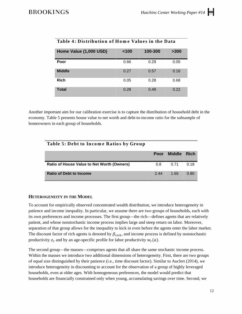
Table 4: Distribution of Home Values in the Data

Home Value (1,000 USD) <100 100-300 >300

Poor 0.66 0.29 0.05

Middle 0.27 0.57 0.16

Rich 0.05 0.28 0.68

Total 0.28 0.49 0.22

Another important aim for our calibration exercise is to capture the distribution of household debt in the economy. Table 5 presents house value to net worth and debt-to-income ratio for the subsample of homeowners in each group of households.

Table 5: Debt to Income Ratios by Group

Poor Middle Rich

Ratio of House Value to Net Worth (Owners) 0.8 0.71 0.18

Ratio of Debt to Income 2.44 1.65 0.80

HETEROGENEITY IN THE MODEL

To account for empirically observed concentrated wealth distribution, we introduce heterogeneity in patience and income inequality. In particular, we assume there are two groups of households, each with its own preferences and income processes. The first group—the rich—defines agents that are relatively patient, and whose nonstochastic income process implies large and steep return on labor. Moreover, separation of that group allows for the inequality to kick in even before the agents enter the labor market. The discount factor of rich agents is denoted by 𝛽𝛽𝑟𝑟𝑖𝑖𝑐𝑐ℎ, and income process is defined by nonstochastic productivity 𝑧𝑧𝑟𝑟 and by an age-specific profile for labor productivity 𝑤𝑤𝑟𝑟(𝑎𝑎).

The second group—the masses—comprises agents that all share the same stochastic income process. Within the masses we introduce two additional dimensions of heterogeneity. First, there are two groups of equal size distinguished by their patience (i.e., time discount factor). Similar to Auclert (2014), we introduce heterogeneity in discounting to account for the observation of a group of highly leveraged households, even at older ages. With homogeneous preferences, the model would predict that households are financially constrained only when young, accumulating savings over time. Second, we

12


also introduce a group of households that always rent houses rather than buying them. These “exogenous renters” make up one-quarter of the masses. Without this type, the model would predict that people rent houses only when young, whereas the data shows a sizeable fraction of renters at all ages. We can think of this group as comprising more mobile households who are likely to switch locations and thus less willing to invest in a house.

Within the masses, labor productivity 𝑧𝑧 follows a four-state Markov process with conditional probabilities Γ𝑧𝑧. The four states are denoted by 𝑧𝑧 ∈ 𝑍𝑍 = 𝑧𝑧1, 𝑧𝑧2, 𝑧𝑧3, 𝑧𝑧4. We normalize efficiency units of youngest poor cohort to 1, so that 𝑧𝑧1 = 1 and 𝑤𝑤𝑛𝑛(1) = 1.

INDEPENDENTLY CALIBRATED PARAMETERS

A subset of the parameters of our model is set individually to match specific targets. To match the sorting of households used in empirical analysis, we assume that a model period lasts 2.5 years, with the youngest cohort corresponding to ages below 25, and the oldest comprising those aged 75 and older. That gives 𝑇𝑇 = 22 model periods with retirement starting at age 65.

We assume that willingness to substitute consumption bundles across time and states is standard 𝛾𝛾 = 2, the weight on housing services consumption is 𝜂𝜂 = 0.2, and the weight on leisure is 𝜎𝜎 = 0.6. The utility weight η determines the expenditure share of housing, for which we target 20 percent of total expenditure. The utility weight σ is chosen to match the standard target for labor supply to be equal to 40 percent of the overall time endowment.

For the downpayment constraint1 − 𝜓𝜓, we use a value of 20 percent for the benchmark calibration in line with Keys et al. (2013); Landvoigt, Piazzesi, and Schneider (2015); and many others.

The risk-free world interest rate is set to 3 percent on an annual basis, so that 𝑖𝑖 = (1.03)2.5 − 1. We abstract from taxation and bequests in this version of the model, but allow for a constant Social Security transfer.

JOINTLY CALIBRATED PARAMETERS

The following set of parameters remains to be determined 𝛽𝛽𝑟𝑟𝑖𝑖𝑐𝑐ℎ, 𝛽𝛽𝐻𝐻, 𝛽𝛽𝐿𝐿 , 𝑧𝑧2, 𝑧𝑧3, 𝑧𝑧4,Γ𝑧𝑧,𝑤𝑤𝑛𝑛(𝑎𝑎), 𝐻𝐻(ℎ), the stochastic income process for the masses, the type and age-specific profile of labor earnings, and the housing stock and qualities. We assume that the large house comprises 20 percent of the housing stock, and the small house 45 percent, leaving 35 percent for the rented house (which matches the homeownership rate in the United States). The service flows from these houses are chosen to match to observed home values for each group discussed above.

The remaining parameters are jointly chosen to approximate a set of target moments, which comprise earnings targets for each group (Table 1), wealth targets (Table 2), leverage targets (Table 5), the fraction of financially constrained households (0.22, from Auclert, 2014) and empirical estimates of the volatility and persistence of the income process for U.S. households in the panel study of income dynamics (PSID) data (Floden and Lindé, 2001). Given these estimates, the income process is discretized with four states using the Tauchen method. The resulting estimated income process is given by:

13


𝑧𝑧1 = 0.833; 𝑧𝑧2 = 0.941; 𝑧𝑧3 = 1.063, 𝑧𝑧4 = 1.2,

with the following transition matrix:

0.6 0.3 0.1 0.01

0.28 0.37 0.26 0.08

0.08 0.26 0.37 0.28

0.02 0.11 0.3 0.57

The earnings displayed in Table 1 cannot be matched exactly because of endogenous labor supply. Table 6 displays steady-state average earnings by group in the calibrated model.

The discount factors that provide the best match to the moments of the wealth distribution are given by 𝛽𝛽𝑟𝑟𝑖𝑖𝑐𝑐ℎ = 1.052.5,𝛽𝛽𝐻𝐻 = . 982.5, and 𝛽𝛽𝐿𝐿 =. 972.5. Notice that the rich are estimated to have a discount factor exceeding 1 to account for high wealth accumulation (a discount factor larger than 1 does not pose a problem here due to finite lifetimes). Also, only a small difference in discounting within the masses is needed to generate realistic indebtedness.

14


Table 6: Relative Earnings in the Model

Age Poor Middle Rich

<25 1.00 1.28 2.70

25-27.5 2.71 3.96 4.68

27.5-30 3.32 3.69 5.27

30-32.5 2.71 3.32 9.67

32.5-35 3.02 4.89 13.33

35-37.5 2.96 4.97 14.05

37.5-40 2.96 5.01 29.04

40-42.5 3.01 4.86 27.43

42.5-45 3.09 4.70 25.40

45-47.5 3.14 4.58 23.05

47.5-50 3.18 4.57 20.35

50-52.5 3.21 4.57 16.93

52.5-55 3.33 4.63 13.09

55-57.5 3.11 4.16 8.90

57.5-60 2.28 3.91 7.41

60-62.5 0.66 1.23 0.00

62.5-65 0.48 0.70 0.00

COMPUTATIONAL EXPERIMENTS Combining the accounting framework and the modeling framework, we are able to carry out a set of experiments to gauge the redistribution effects of various monetary policy measures. Our main focus is on redistribution arising from changes in inflation. Here we consider two polar scenarios. The first is a sudden inflation shock (i.e., an unanticipated rise in the price level without changes in expected future inflation). While this is not the most empirically plausible type of shock, it is useful to provide intuition on the overall exposure to nominal price changes in the economy. Given the accounting framework, we can compute the wealth change for each sector and group of households that would be generated by such a shock. With the quantitative (and calibrated) modeling framework, we can feed the redistribution

15


shock into the model as a shock that displaces the economy from its balanced growth path, and then assess the macroeconomic and welfare consequences of this change over time, for each group and sector and for the economy as a whole.

In the same way, we can assess the consequences of a shock to inflation expectations (i.e., changes in the price levels that are anticipated). Holding the real interest rate fixed, an inflation expectation shock shifts the nominal term structure in a deterministic way. Given the streams-of-payment representation of assets in the accounting framework, we can then revalue each group’s portfolio to compute redistribution effects, which then become inputs in the quantitative analysis.

The unanticipated and anticipated inflation experiments are carried out under the assumption of a constant real interest rate. It is interesting to compare the responses to our thought experiment to a change in real interest rates. We therefore carry out an additional experiment where real interest rates are reduced for a few years. We can think of this experiment as corresponding to a change in world credit market conditions, in particular a strengthening of the “global savings glut” that some consider an important factor in the buildup to the Great Recession.

AN UNANTICIPATED INFLATION SHOCK

The first experiment we consider is an unanticipated inflation shock. The economy starts out in the steady state. Then households are confronted with a surprising one-time jump in the price level. From that point forward, inflation is at the same level that was expected initially, so that nominal interest rates are unchanged. Redistribution occurs because a jump in the price level proportionally lowers the real value of all nominal assets and liabilities. To make the experiment comparable to the anticipated inflation shock considered below, we set the size of the jump to the cumulative additional inflation that would result if the inflation rate rose by 5 percentage points per year over a 10-year horizon. This inflation shock amounts to a jump in the price level by about 65 percent or, equivalently, a decrease in the real value of all nominal assets and liabilities by about 40 percent. While such a jump in the price level is not in itself a realistic policy scenario, the unanticipated inflation shock also captures the consequences from repeated surprises. Specifically, the unanticipated shock provides an assessment of the redistribution consequences if inflation were to rise by 5 percent per year but households did not adjust inflation expectations at all. Together with the anticipated scenario considered below (where expectations adjust immediately), the two scenarios provide upper and lower bounds for the redistribution arising from a sustained inflation episode. The example of the 1970s suggests that expectations can be slow to catch up with actual inflation, so allowing for the possibility of repeated surprises is important.

Figure 2 displays the aggregate wealth changes that each group of households experienced as a result of the inflation shock. We group households in two dimensions. The first dimension is age—2.5-year brackets from under 25 to 75 and older. Within each age cohort, we distinguish three groups. We separately consider the rich group (i.e., the top 10 percent of the wealth distribution within each age group). Among the non-rich, we distinguish between renters and homeowners. This distinction is essential because among the non-rich, mortgage borrowing is the dominant source of exposure to inflation risk. In the model, the group of renters consists of the “exogenous renters” who always rent houses, and other non-rich who aspire to be future homeowners, but are renting temporarily. For each

16


group, the total wealth change is expressed as a fraction of annual GDP.

The figure shows that for renters of all ages, the aggregate redistribution effect of an inflation shock is essentially zero. For lack of homes, renters do not have mortgages, and thus do not gain from deflating the real value of debt. Renters do have other forms of debt and some nominal savings, but in aggregate these positions are small compared to the mortgage debt of homeowners and the nominal assets of the rich.

Figure 2: Total Wealth Change for Different Groups of Households after Unanticipated Inflation Shock

Middle-class homeowners are the main winners from inflation, and particularly so from about 35 to 50 years of age (in middle age). Their gains are quantitatively large and exceed 1 percent of GDP for many groups (recall that each age group of middle-class homeowners makes up only about 3 percent of households). This is because these households are generally highly leveraged, with many holding mortgages that are far larger than household net worth. Gains decline at older ages because older households have often repaid most (or all) of their mortgage. The oldest homeowners are usually debt-free and have nominal savings, so their wealth declines after an inflation shock.

The main losers from inflation are the old rich. This group accounts for the bulk of savings in the economy, including nominal savings in terms of savings accounts, bonds, and other nominal assets. Thus, in the aggregate, the inflation shock mainly amounts to a wealth transfer from the old rich to middle-class and middle-aged homeowners.

We now introduce the wealth changes displayed in Figure 2 as an unexpected shock to the steady state of our economy. The groups for which we compute redistribution total are not homogeneous; the non-rich are subject to income shocks and also differ in patience. We assign the wealth change in each group in proportion to the financial assets of a household. Figure 3 displays the impact of this redistribution shock on the aggregate consumption and output of the economy over the first 25 years after the shock in partial equilibrium (i.e., holding wages, real interest rates, and fixed house prices). In the period of the shock, nondurable consumption declines by about 3 percent, and output declines by about 1 percent.

17


Subsequently, both series slowly converge back to their steady-state values.

Figure 3: Reaction of Aggregate Consumption and Output to Unanticipated Inflation Shock with Fixed House Prices

One central feature of this transition path is that the changes induced by redistribution are long lived. The duration of monetary policy effects that are due to nominal frictions are usually measured in quarters. In contrast, the changes in consumption and output generated by redistribution are present for about 20 years. The reason is that the wealth changes brought about by the shock disappear only as cohorts age and are replaced by younger cohorts unaffected by the shock, which is a slow process. Thus, even effects that are moderate in impact have a large cumulative impact on the economy.

Changes in consumption arise because winners and losers from inflation react differently to wealth changes. In our model, the marginal propensity to consume is driven by three factors. First, people differ in terms of patience (discount factors). Second, the degree to which borrowing constraints bind varies across households. Third, age differences affect the propensity to consume. Generally, older people smooth their wealth shock over a shorter number of remaining periods.

Given that the losers from inflation are mostly the rich, in terms of patience and exposure to financial constraints they tend to have a lower marginal propensity to consume. However, the effect that turns out to dominate is age. The winners (middle-class mortgage borrowers) are much younger than the losers, which leads to a lower propensity to consume.

18


Figure 4: Reaction of Labor Supply to Unanticipated Inflation Shock with Fixed House Prices

The effects on output are driven by labor supply. Leisure is a normal good in our model, so that households who experience a windfall gain work less. What is significant for the overall effect is that many of the winners are old and hence retired, which limits the ability of the losers from inflation to react by increasing labor supply. Figure 4 breaks down the change in labor supply by the three main groups: renters, middle-class homeowners, and the rich. The absolute change in labor supply is largest for the middle-class homeowners, who also make up the largest fraction of the population (and of effective labor supply). Compared to their wealth loss, the change in labor supply by the rich is small, which is mostly due to retirement.

The experiment considered in Figures 3 and 4 is under partial equilibrium (i.e., implicitly we assume that there is a flexible supply of each type of house at the steady state price). Figure 5 shows how the demand for small and large houses evolves after the shock. We observe a large rise in the demand for large houses, and a smaller decline in the demand for small houses. The increase in demand for large houses is due to windfall gains for existing homeowners. Most of these homeowners are in small houses, and the windfall gain allows many of them to upgrade to a large house. This effect increases the demand for large houses and correspondingly lowers the demand for small houses. The change for large houses is proportionally larger because there are fewer large houses in total.

19


Figure 5: Reaction of Housing Demand to Unanticipated Inflation Shock with Fixed House Prices

Figure 6 shows how the lifetime welfare of each cohort alive at the time of the shock is affected by the redistribution shock. The welfare changes are expressed in equivalent nondurable consumption units. For example, a welfare change of 0.01 means that a household experiences a gain after the shock such that nondurable consumption throughout the remaining lifetime would have to be cut by 1 percent to move utility back to the steady-state level. Given that there is heterogeneity within groups (due to income shocks and differences in preferences), these changes are computed by aggregating welfare within each group with equal welfare weights. The most important feature to notice about Figure 6 is that the welfare changes for particular groups are enormous in size when compared to typical welfare effects from policy changes. Many groups of middle-class homeowners gain more than 5 percent in welfare, whereas the oldest rich cohorts lose close to 15 percent. Generally, welfare effects are larger at older ages because older households can smooth out their gains or losses over fewer periods, which increases the per-period welfare impact.

20


Figure 6: Effect on Welfare of Unanticipated Inflation Shock with Fixed House Prices (Measured in Nondurable Consumption Units)

Next, we consider how outcomes change if we allow for general equilibrium in the housing market. The economy is still a small, open economy to the extent that interest rates and wages are set in world markets; however, small and large houses are now in fixed supply (at the steady state value), and house prices have to adjust to clear the market. Figure 7 shows how house prices evolve after the unanticipated inflation shock. We observe a sustained rise in the price of large houses, but barely any change in the price of small houses. Concerning the price of large houses, changes in demand are driven by windfall gains to owners of small houses whose mortgage got devalued in real terms. As a result, more owners desire to upgrade to a large house, which drives up the price. While at the same time the old rich experience losses, given their high wealth these losses are not sufficient to induce them to downgrade at the same time (although with more housing types, we would observe declines for the prices of large mansions).

21


Figure 7: Reaction of House Prices to Unanticipated Inflation Shock

Regarding the flat price of small houses, there are two effects to consider. In Figure 6 under partial equilibrium, we observe a decline in the demand for small houses, driven by upgrading to large houses among winners from redistribution. However, under general equilibrium the supply of large houses is fixed, and potential upgraders are priced out of that market so that this change in demand is prevented. The second effect comes through wealth changes for potential future house buyers. If current renters looking to buy their first house experienced wealth gains, this would drive up the price of small houses. However, precisely because future first-time buyers are current renters, they do not have a mortgage, and thus gain little or nothing from inflation. Hence, wealth changes for future buyers are small, resulting in flat prices.

Quantitatively, the change in the price of large houses is moderate, with an increase of 1.5 percent in period of the shock, with prices returning to steady state over the next 20 to 23 years. The small reaction is in part explained by the assumption of perfect foresight in computing the transition path. Potential buyers are aware that prices will decline in the future, which increases the value of waiting to buy a house. The option value effect makes demand elastic with respect to the current price.

In summary, regarding the housing market we find that inflation-induced redistribution affects prices in a sustained and asymmetric way. Prices for homes typically bought by first-time buyers are predicted to move little. The largest price effects would be expected to occur for houses that are in demand by relatively young upgraders with high outstanding mortgages, because these households experience the largest gains relative to their net worth.

Figures 8 and 9 display how consumption, output, and labor supply evolve in general equilibrium. Compared to the partial equilibrium case, the main changes are that the drop in consumption is now smaller, whereas the drop in output is larger. Under partial equilibrium, a sizeable portion of the gains for the middle-class homeowners were used for buying bigger houses. This adjustment cannot happen under general equilibrium, and instead households buy more nondurable goods and enjoy more leisure.

22


Figure 8: Reaction of Aggregate Consumption and Output to Unanticipated Inflation Shock with Endogenous House Prices

Figure 9: Reaction of Labor Supply to Unanticipated Inflation Shock with Endogenous House Prices

Conversely, some of the drop in consumption for the old rich is now mitigated by being able to sell their large houses at higher prices.

In terms of welfare, Figure 20 shows the main differences. The younger, middle-class homeowners experience smaller gains, and the old rich experience smaller losses. Both effects are explained by the rise in the price for large houses, for which the old rich are sellers and the middle-class homeowners are buyers.

A Shift in Anticipated Future InflationWe now proceed to the anticipated inflation experiment. In this scenario a new inflation path is suddenly announced, and nominal interest rates adjust to fully reflect this

23


change. After the initial change in the inflation path, there are no further surprises: all households perfectly anticipate the rise in future inflation. This experiment amounts to an unanticipated change to the inflation target in an inflation-targeting regime that is fully reflected in market expectations. This experiment is particularly relevant in the current policy environment because concerns about the zero lower bound have led to calls to consider a moderately higher inflation target. In the experiment, inflation is raised by 5 percentage points over a 10-year horizon.

Figure 10: Effect on Welfare of Unanticipated Inflation Shock with Endogenous House Prices (Measured in Nondurable Consumption Units)

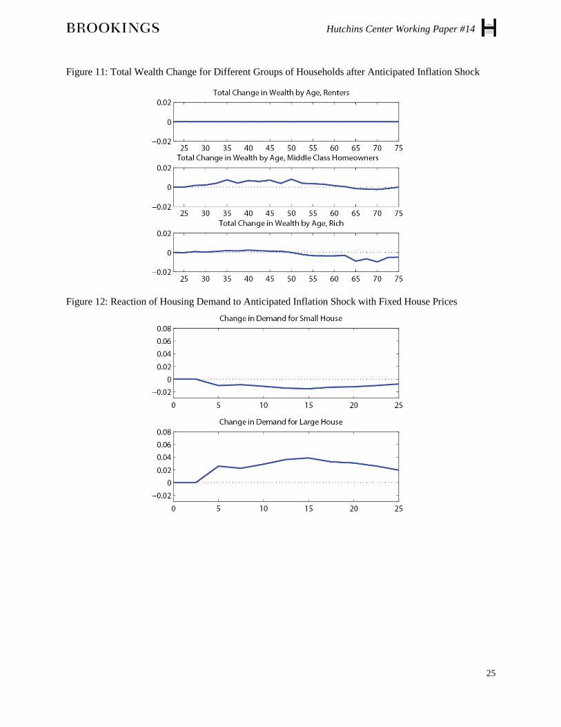
Figure 11 displays the redistribution total for the anticipated inflation change. Compared to Figure 2, what is notable is that the gains for middle-class homeowners are similar in magnitude, whereas the losses for the old rich are smaller under the anticipated inflation change. This difference is due to maturities. Much of mortgage debt is long term (the most common contract is still a 30-year, fixed-rate mortgage), whereas the nominal assets of the rich have a shorter average duration. Assets with a short maturity have a lower exposure to inflation risk because they can be reinvested at the raised nominal rates once the asset matures.

Figures 12 and 13 display the demand for houses under partial equilibrium, and the price for houses under general equilibrium for the anticipated inflation shock. The reactions of demand and equilibrium price are qualitatively similar to the case of the unanticipated shock. In terms of magnitude, the size of the adjustments is reduced, but only by a small amount. Intuitively, the changes in the housing market are primarily driven by the gains to middle-class mortgage borrowers, and because mortgages are long term, the gains for this group are similar in size for both experiments.

24


Figure 11: Total Wealth Change for Different Groups of Households after Anticipated Inflation Shock

Figure 12: Reaction of Housing Demand to Anticipated Inflation Shock with Fixed House Prices

25


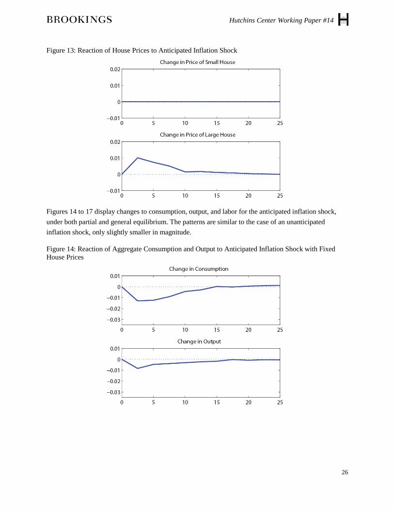
Figure 13: Reaction of House Prices to Anticipated Inflation Shock

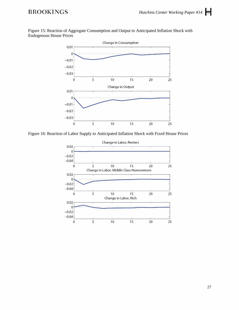
Figures 14 to 17 display changes to consumption, output, and labor for the anticipated inflation shock, under both partial and general equilibrium. The patterns are similar to the case of an unanticipated inflation shock, only slightly smaller in magnitude.

Figure 14: Reaction of Aggregate Consumption and Output to Anticipated Inflation Shock with Fixed House Prices

26


Figure 15: Reaction of Aggregate Consumption and Output to Anticipated Inflation Shock with Endogenous House Prices

Figure 16: Reaction of Labor Supply to Anticipated Inflation Shock with Fixed House Prices

27


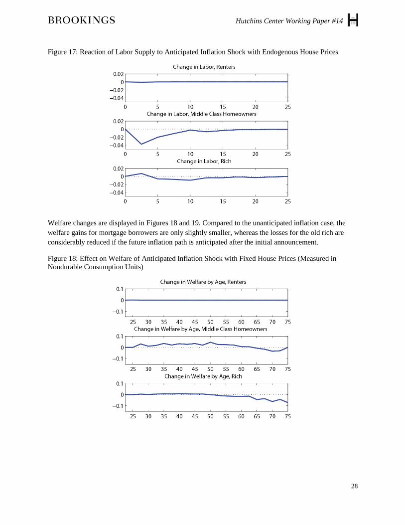
Figure 17: Reaction of Labor Supply to Anticipated Inflation Shock with Endogenous House Prices

Welfare changes are displayed in Figures 18 and 19. Compared to the unanticipated inflation case, the welfare gains for mortgage borrowers are only slightly smaller, whereas the losses for the old rich are considerably reduced if the future inflation path is anticipated after the initial announcement.

Figure 18: Effect on Welfare of Anticipated Inflation Shock with Fixed House Prices (Measured in Nondurable Consumption Units)

28


Figure 19: Effect on Welfare of Anticipated Inflation Shock with Endogenous House Prices (Measured in Nondurable Consumption Units)

A REAL INTEREST RATE SHOCK

We now move on to an experiment where real interest rates change. Specifically, we consider a scenario of a drop in the real rate by 1 percentage point (100 basis points) over 10 years. Formally, our model is a small, open economy, so this experiment can be interpreted as capturing the redistribution and aggregate implications of a change in world interest rates such as the one driven by the global savings glut. However, to the extent that conventional or unconventional monetary policy is able to affect real rates, some of the effects captured here would also be relevant for monetary policy decisions.

Figures 20 and 21 display how the demand for houses under partial equilibrium and the price for houses under general equilibrium evolve after the decline in real interest rates. In this experiment there is no immediate wealth change, but current or future homeowners still gain because home ownership becomes more affordable. Changes in housing demand can occur because lower interest rates immediately lower the cost of buying a house, and also because lower interest rates over time lead to a wealth increase for initially indebted households. The cost effect would be largest at the beginning of the episode (because then interest rates are lower for more future periods), whereas the wealth effect would increase with the duration of the episode (as saved interest expenses accumulate). Figure 20 shows that the increase in demand is largest after 10 years—at the end of the period of low interest rates—suggesting that the wealth effect is dominant. Consistent with this interpretation, we see much larger gains in the price of larger houses. For these houses, the wealth effect would be larger because the potential buyers of larger houses usually have mortgages on small houses, and thus have more to gain from lower interest rates than current renters who think about buying a small house. Quantitatively, the rise in the price of large houses is much larger than in either of the inflation experiments.

29


Figure 20: Reaction of Housing Demand to Real Interest Rate Shock with Fixed House Prices

Figure 21: Reaction of House Prices to Real Interest Rate Shock

Figures 22 to 25 show how consumption, output, and labor supply evolve under lower interest rates, for both partial and general equilibrium. In both cases, consumption rises, whereas output and labor supply fall after the decline in the real interest rates. Compared to the redistribution experiments, the changes are less persistent. All series are close to their steady-state values after interest rates return to their original level after the end of the10-year episode. The change in interest rates does have redistributive implications, but these are not sufficiently large to give rise to large persistence.

The movements in nondurable consumption, output, and labor occur because the decline in the real interest rates makes immediate consumption (of goods or leisure) more attractive compared to future consumption. The movements in labor suggest that middle-class homeowners gain a lot from the

30


reduced real cost of their mortgages. However, now there is also a large positive effect on young renters, because for them moving up to owning a house becomes more affordable.

Comparing partial and general equilibrium results, we find that under general equilibrium the movements in nondurable consumption, labor, and output are much larger than under partial equilibrium. This is because under partial equilibrium the gain in large part flows into an expanded demand for housing. With a fixed supply of housing, the gains have to show up somewhere else, namely in increased nondurable consumption and increased leisure.

Figure 22: Reaction of Aggregate Consumption and Output to Real Interest Rate Shock with Fixed House Prices

Figure 23: Reaction of Aggregate Consumption and Output to Real Interest Rate Shock with Endogenous House Prices

31


Figure 24: Reaction of Labor Supply to Real Interest Rate Shock with Fixed House Prices

Figure 25: Reaction of Labor Supply to Real Interest Rate Shock with Endogenous House Prices

Figures 26 and 27 show how the welfare of the cohorts alive in the shock period is affected by lower interest rates. All renters experience a small improvement in welfare. Welfare improvements are also observed for all middle-class homeowners, with quantitatively large effects that exceed 10 percent in consumption units in some cases. Changes in welfare for the rich are small. The largest reductions are observed for the rich aged 45 to 65 who have accumulated a large stock of assets, the return of which is reduced by the reduction in the real rate. Comparing partial equilibrium and general equilibrium, the largest difference is that the old rich are much better off under general equilibrium. This is because this group benefits from the large increase in the price of large houses, which the rich sell at the end of their life cycle.

32


Figure 26: Effect on Welfare of Real Interest Rate Shock with Fixed House Prices (Measured in Nondurable Consumption Units)

Figure 27: Effect on Welfare of Real Interest Rate Shock with Endogenous House Prices (Measured in Nondurable Consumption Units)

CONCLUSIONS We have examined the redistribution implications of monetary policy changes in a rich life cycle model that features preference and income heterogeneity, income risk, and a rich housing market with different segments for rental units and small and large owner-occupied houses. We have used this framework to examine the redistributive repercussions of changes in monetary policy, such as the adoption of a higher inflation target that leads to a devaluation of existing nominal assets and liabilities.

33


A first conclusion from our work is that redistribution effects are quantitatively large. For many groups, the change in welfare is an order of magnitude larger than welfare effects of monetary changes in models that abstract from heterogeneity and redistribution. The effects are also highly heterogeneous in the population, with large losses from inflation for older, rich households with large investments in long-term nominal assets (such as bonds), and large gains for middle-class homeowners with large outstanding mortgages. If nothing else, these findings suggest that changes in the monetary regime should be politically contentious, and call for an examination of the political economy of monetary policy.

In terms of effects on aggregates, our results for inflation experiments suggest that a sustained rise in inflation has a dampening effect on demand for nondurable consumption, as well as on output. These effects are moderate in size of impact, but are also extremely persistent, leading to large cumulative changes. Hence, while inflation may have a stimulating effect on aggregates through other mechanisms (such as short-run nominal rigidities), the redistribution effect tends to pull in the opposite direction.

A key innovation of our framework is a rich housing market that allows us to assess the effects of inflation-induced redistribution on housing demand and house prices. Here we find that inflation-induced redistribution can stimulate housing demand, but generally not in the segment of the market populated by first-time buyers. Windfall gains from inflation accrue to existing mortgage borrowers, not to potential future buyers who are currently renting. Thus, inflation-induced redistribution tilts house prices towards higher prices for higher-value segments.

34


35

REFERENCES Adam, Klaus, and Junyi Zhu, 2015. “Price Level Changes and the Redistribution of Nominal Wealth

Across the Euro Area.” Forthcoming. Journal of the European Economic Association.

Albanesi, Stefania, 2006. “Inflation and Inequality.” Journal of Monetary Economics.

Auclert, Adrien, 2015. “Monetary Policy and the Redistribution Channel.” Job Market Paper. MIT.

Benigno, Pierpaolo, Gauti B. Eggertsson, and Federica Romei, 2014. “Dynamic Debt Deleveraging and Optimal Monetary Policy.” Working Paper No. 20556. National Bureau of Economic Research.

Bohn, Henning, 1988. “Why Do We Have Nominal Government Debt?” Journal of Monetary Economics, Vol. 21(1), pp. 127–140.

——, 1990. “Tax Smoothing with Financial Instruments.” The American Economic Review, Vol. 80(5), pp. 1,217–1,230.

Burnside, Craig, Martin Eichenbaum, and Sergio Rebelo, 2006. “Government Finance in the Wake of Currency Crises.” Journal of Monetary Economics, Vol. 53(3), pp. 401–40.

Chatterjee, Satyajit, and Burcu Eyigungor, 2015. “Quantitative Analysis of the U.S. Housing and Mortgage Markets and the Foreclosure Crisis.” Forthcoming. Review of Economic Dynamics.

Coibion, Olivier, Yuriy Gorodnichenko, Lorenz Kueng, and John Silvia, 2012. “Innocent Bystanders? Monetary Policy and Inequality in the U.S.” Working Paper No. 18170. National Bureau of Economic Research.

Doepke, Matthias, and Martin Schneider, 2006a. “Aggregate Implications of Wealth Redistribution: The Case of Inflation.” Journal of the European Economic Association, Vol. 4(2–3), pp. 493–502.

——, 2006b. “Inflation and the Redistribution of Nominal Wealth.” Journal of Political Economy, Vol. 114(6), pp. 1,069–1,097.

——, 2006c. “Inflation as a Redistribution Shock: Effects on Aggregates and Welfare.” Working Paper No. 12319. National Bureau of Economic Research.

Erosa, Andrés, and Gustavo Ventura, 2002. “On Inflation as a Regressive Consumption Tax.” Journal of Monetary Economics, Vol. 49(4), pp. 761–795.

Floden, Martin, and Jesper Lindé, 2001. “Idiosyncratic Risk in the United States and Sweden: Is There a Role for Government Insurance?” Review of Economic Dynamics, Vol. 4(2), pp. 406–437.

Garriga, Carlos, Finn E. Kydland, and Roman Sustek, 2013. “Mortgages and Monetary Policy.” Working Paper No. 19744. National Bureau of Economic Research.


36

Glover, Andrew, Jonathan Heathcote, Dirk Krueger, and José-Víctor Ríos-Rull, 2011. “Intergenerational Redistribution in the Great Recession.” Working Paper No. 16924. National Bureau of Economic Research.

Hedlund, Aaron, 2015. “Failure to Launch: Housing, Debt Overhang, and the Inflation Option During the Great Recession.” Working Paper. University of Missouri.

Kaplan, Greg, and Giovanni L. Violante, 2014. “A Model of the Consumption Response to Fiscal Stimulus Payments.” Econometrica, Vol. 82(4), pp. 1,199–1,239.

Keys, Benjamin J., Tomasz Piskorski, Amit Seru, and Vikrant Vig, 2013. “Mortgage Financing in the Housing Boom and Bust.” In Housing and the Financial Crisis, pp. 143–204, edited by Edward L. Glaeser and Todd Sinai. NBER Conference Report Series. University of Chicago Press.

Koenig, Evan F., 2013. “Like a Good Neighbor: Monetary Policy, Financial Stability, and the Distribution of Risk.” International Journal of Central Banking, Vol. 9(2), pp. 57–82.

Landvoigt, Tim, Monika Piazzesi, and Martin Schneider, 2015. “The Housing Market(s) of San Diego.” American Economic Review, Vol. 105(4), pp. 1,371–1,407.

Lee, Jae Won, 2014. “Monetary Policy with Heterogeneous Households and Imperfect Risk-Sharing.” Review of Economic Dynamics, Vol. 17(3), pp. 505–522.

Meh, Césaire, José-Víctor Ríos-Rull, and Yaz Terajima, 2010. “Aggregate and Welfare Effects of Redistribution of Wealth under Inflation and Price-Level Targeting.” Journal of Monetary Economics, Vol. 57(6), pp. 637–652.

Meh, Césaire, and Yaz Terajima, 2011. “Inflation, Nominal Portfolios, and Wealth Redistribution in Canada.” Canadian Journal of Economics, Vol. 44(4), pp. 1,369–1,402.

Neumeyer, Pablo Andres, 1998. “Inflation-Stabilization Risk in Economies with Incomplete Asset Markets.” Journal of Economic Dynamics and Control, Vol. 23(3), pp. 371–91.

Persson, Mats, Torsten Persson, and Lars E. O. Svensson, 1998. “Debt, Cash Flow and Inflation Incentives: A Swedish Example.” In The Debt Burden and Its Consequences for Monetary Policy, edited by Guillermo Calvo and Mervyn King, pp. 28–62. New York: St. Martin’s Press.

Pescatori, Andrea, 2007. “Incomplete Markets and Households’ Exposure to Interest Rate and Inflation Risk: Implications for the Monetary Policy Maker.” Working Paper 709. Federal Reserve Bank of Cleveland.

Sheedy, Kevin D., 2014. “Debt and Incomplete Financial Markets: A Case for Nominal GDP Targeting.” Brookings Papers on Economic Activity, Spring, pp. 301–361.

Sterk, Vincent, and Silvana Tenreyro, 2014. “The Transmission of Monetary Policy Operations through Redistributions and Durable Purchases.” Unpublished Paper. London School of Economics and Political Science.

distributional effects of monetary policy · redistribution from lenders to borrowers implies that...

Documents