distribution system line models...the phase impedance and phase admittance matrices without assuming...
TRANSCRIPT

FAKULTA ELEKTROTECHNIKY A KOMUNIKAČNÍCH TECHNOLOGIÍ
VYSOKÉ UČENÍ TECHNICKÉ V BRNĚ
Distribution System Line Models
Authors:
Ing. Mayada Daboul doc. Ing. Jaroslava Orságová, Ph.D.
May 2013
ePower – Inovace výuky elektroenergetiky a silnoproudé elektrotechniky formou e-learningu a rozšíření prakticky orientované výuky
OP VK CZ.1.07/2.2.00/15.0158

1 Distribution System Line Models
The modeling of distribution overhead and underground line segments is a critical step
in the analysis of a distribution feeder. It is important to include the actual phasing of the line
and the correct spacing between conductors.
The phase impedance and phase admittance matrices without assuming transposition of the lines will be used in the models for overhead and underground line segments.
1.1 Exact Line Segment Model
The exact model of a three-phase, two-phase, or single-phase overhead or underground line is shown in Figure 1.1.
Some of the impedance and admittance values will be zero when a line segment is two-
phase or single-phase.
For the line segment of Figure 1.1, the equations relating the input (node n) voltages and currents to the output (node m) voltages and currents are developed as follows:
Kirchhoff’s current law applied at node m
[
]
[
]
[
] [
]
(1.1)
in condensed form equation 1.1 becomes
[ ] [ ]
[ ] [ ] (1.2)
Kirchhoff’s voltage law applied to the model gives
[
]
[
]
[
] [
]
(1.3)
in condensed form Equation 1.3 becomes
[ ] [ ] [ ] [ ] (1.4)
Substituting Equation 1.2 into Equation 1.4
[ ] [ ] [ ] {[ ]
[ ] [ ] } (1.5)
collecting terms
[ ] {[ ]
[ ] [ ]} [ ] [ ] [ ] (1.6)
where
[ ] [
] (1.7)
Distribution System Line Models 3
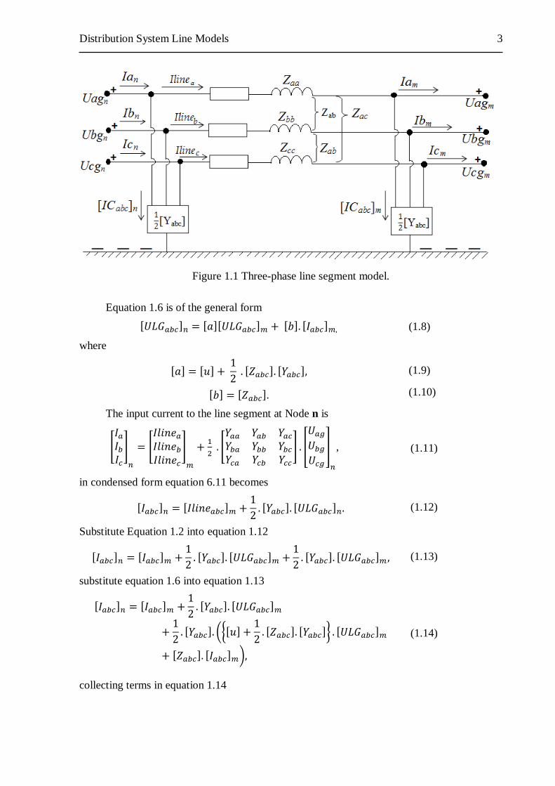
Figure 1.1 Three-phase line segment model.
Equation 1.6 is of the general form
[ ] [ ][ ] [ ] [ ] (1.8)
where
[ ] [ ]
[ ] [ ] (1.9)
[ ] [ ] (1.10)
The input current to the line segment at Node n is
[
]
[
]
[
] [
]
, (1.11)
in condensed form equation 6.11 becomes
[ ] [ ]
[ ] [ ] (1.12)
Substitute Equation 1.2 into equation 1.12
[ ] [ ]
[ ] [ ]
[ ] [ ] (1.13)
substitute equation 1.6 into equation 1.13
[ ] [ ]
[ ] [ ]
[ ] ({[ ]
[ ] [ ]} [ ]
[ ] [ ] )
(1.14)
collecting terms in equation 1.14

[ ] {[ ]
[ ][ ] [ ]} [ ]
{[ ]
[ ] [ ]} [ ]
(1.15)
Equation 1.15 is of the form
[ ] [ ] [ ] [ ] [ ] (1.16)
where
[ ] [ ]
[ ][ ] [ ] (1.17)
[ ] [ ]
[ ] [ ]
(1.18)
Equations 1.8 and 1.16 can be put into partitioned matrix form
[[ ] [ ]
] [[ ] [ ]
[ ] [ ]] [
[ ] [ ]
] (1.19)
To solve the voltages and currents at Node m in terms of the voltages and currents at
node n, equation 1.19 must be turned around:
[[ ] [ ]
] [[ ] [ ]
[ ] [ ]]
[[ ] [ ]
]. (1.20)
The inverse of the abcd matrix is simple because the determinant is:
[ ] [ ] [ ] [ ] [ ] (1.21)
Using the relationship of Equation 1.21, Equation 1.20 becomes:
[[ ] [ ]
] [[ ] [ ]
[ ] [ ]]
[[ ] [ ]
] (1.22)
Since the matrix [a] is equal to the matrix [d], equation 1.22 in expanded form becomes:
[ ] [ ] [ ] [ ] [ ] (1.23)
[ ] [ ] [ ] [ ] [ ] (1.24)
Sometimes it is necessary to compute the voltages at Node m as a function of the
voltages at Node n and the currents entering Node m.
Solving Equation 1.8 for the bus m voltages gives
[ ] [ ] {[ ] [ ] [ ] } (1.25)
Equation 1.25 is of the form
[ ] [ ] [ ] [ ] [ ] (1.26)
where
[ ] [ ] (1.27)
[ ] [ ] [ ] (1.28)
The line-to-line voltages are computed by

Distribution System Line Models 5
[
]
[
] [
]
[ ] [ ] (1.29)
where:
[ ] [
] (1.30)
Because the mutual coupling between phases on the line segments is not equal, there
will be different values of voltage drop on each of the three phases. As a result, the voltages
on a distribution feeder become unbalanced even when the loads are balanced. A common
method of describing the degree of unbalance is to use the National Electrical Manufacturers
Association (NEMA) definition of voltage unbalance as given in equation 1.31
| |
| |
(1.31)
Example 1.1
An overhead three-phase distribution line consisting of single conductors arranged
unsymmetrically as shown in Figure 1. Determine the phase impedance matrix and the positive and zero sequence impedances of the line.
The phase conductors are 97-AL1/56-ST1A.
For 97-AL1/56-ST1A D=16mm 𝜌=0.2992 𝛺/km=0.4815 𝛺/mile
( )[ ( ) ]
GMR: the geometric mean radius of conductor.
GMD: the geometric mean distance between conductors.
GMR= r.e-1/4
=0.7788r =0.7788∙8 = 6.2304 mm=0.020441 ft
√
Applying the modified Carson’s equation for self-impedance, the self-impedance for phase A is:
[
]
[
]
where:
ω = 2πf system angular frequency in radians per second,
G = 0.1609344 × 10⁻³
Ω/mile
ƒ= system frequency in Hertz =50Hz

ρ = resistivity of earth in Ω.m =100 Ω.m
0.5609 + j1.1155.
[
]𝛺
The mutual impedance between phases a and b:
[
]
[
]
The primitive impedance matrix in partitioned form is
[ ] [
]
[
]
[ ] [
]
[ ] [ ]
[ ] [ ]
The phase impedance matrix:
[ ] [ ] [ ] [ ] [ ]
[ ] [
]

Distribution System Line Models 7
Figure 1.2 : Overhead conductor arrangement in 22 kV network
A balanced three-phase load of 6000 kVA, 22 kV, 0.9 lagging power factor is being
served at node m of a 5km three-phase line segment.
Determine the generalized line constant matrices [a], [b], [c], and [d].
Using the generalized matrices, determine the line-to-ground voltages and line currents at the source end (node n) of the line segment.
The phase impedance matrix and the shunt admittance matrix for the line segment as computed are:
[ ] [
]
[ ] [
]
SOLUTION:
For the 5km long line segment, the total phase impedance matrix and shunt admittance
matrix are:
[ ] [
]
[ ] [
]
It should be noted that the elements of the phase admittance matrix are very small. The generalized matrices computed according to Equations 1.9, 1.10, 1.17, and 1.18 are:
[ ] [ ]
[ ] [ ] [
]

[ ] [ ] [
]
[ ] [
]
[ ] [
]
[ ] [
]
[ ] [ ] [ ] [
]
Because the elements of the phase admittance matrix are so small, the [a] and [d]
matrices appear to be the unity matrix. If more significant figures are displayed, the [1,1] element of these matrices is:
a1,1 =A11= 0.99999117 + j0.00000395
Also, the elements of the [c] matrix appear to be zero. Again, if more significant figures
are displayed, the 1, 1 term is:
c1,1 = – 0.0000044134 + j0.0000127144
The point here is that for all practical purposes, the phase admittance matrix can be neglected.
The magnitude of the line-to-ground voltage at the load is:
√
Selecting the phase-a-to-ground voltage as reference, the line-to-ground voltage matrix at the load is:
[
]
[
]
The magnitude of the load currents is:
| |
√
For a 0.9 lagging power factor, the load current matrix is
[ ] [
]
The line-to-ground voltages at Node n are computed to be
[ ] [ ] [ ] [ ] [ ] [
] [
]

Distribution System Line Models 9
It is important to note that the voltages at Node n are unbalanced even though the
voltages and currents at the load (Node m) are perfectly balanced. This is a result of the
unequal mutual coupling between phases. The degree of voltage unbalance is of concern
since, for example, the operating characteristics of a three-phase induction motor are very sensitive to voltage unbalance.
Using the NEMA definition for voltage unbalance (equation 1.29), the voltage
unbalance is:
| | | |
| | | |
Although this may not seem like a large unbalance, it does give an indication of how the
unequal mutual coupling can generate an unbalance. It is important to know that NEMA
standards require that induction motors be de-rated when the voltage unbalance exceeds 1.0%.
Selecting rated line-to-ground voltage as base (7199.56), the per-unit voltages at bus n are
[
]
[
] [
]
The line currents at node n are computed to be
[ ] [ ] [ ] [ ] [ ] [
]
Comparing the computed line currents at node n to the balanced load currents at node
m, a very slight difference is noted that is another result of the unbalanced voltages at node n and the shunt admittance of the line segment.
1.1 Modified Line Model
When the shunt admittance of a line is so small, it can be neglected. Figure 1.2 shows
the modified line segment model with the shunt admittance neglected.
When the shunt admittance is neglected, the generalized matrices become:
[ ] [ ] (1.32)
[ ] [ ] (1.33)
[ ] [ ] (1.34)
[ ] [ ] (1.35)
[ ] [ ] (1.36)
[ ] [ ] (1.37)

Figure 1.2 Three-phase line segment model.
1.2 Three Wire Delta Line
If the line is a three-wire delta, then voltage drops down the line must be in terms of the
line-to-line voltages and line currents. However, it is possible to use “equivalent” line-to-
neutral voltages so that the equations derived to this point will still apply. Writing the voltage
drop equations in terms of line to- line voltages for the line in Figure 1.2 results in:
[
]
[
]
[
] [
] (1.38)
where:
[
] [
] [
] (1.39)
Expanding Equation 1.38 for phase a-b:
(1.40)
but
(1.41)
Substitute Equations 1.41 into Equation 6.40
(1.42)
Equation 1.40 can be broken into two parts in terms of equivalent line-toneutral
voltages:
(1.43)

Distribution System Line Models 11
The conclusion here is that it is possible to work with equivalent line-toneutral voltages
in a three-wire delta line. This is very important since it makes the development of general analyses techniques the same for four wire wye and three-wire delta systems.
Example 1.2
The line of Example 1.1 will be used to supply an unbalanced load at node m. Assume
that the voltages at the source end (Node n) are balanced three-phase at 22 kV line-to-line.
The balanced line-to-ground voltages are
[ ] [
]
The unbalanced currents measured at the source end are given by:
[
]
[
]
Determine the line-to-ground and line-to-line voltages at the load end (node m) using
the modified line model. Determine also the voltage unbalance and the complex powers of the load.
SOLUTION
The [A] and [B] matrices for the modified line model are
[ ] [ ] [
]
[ ] [ ] [
]𝛺
Since this is the approximate model,[Iabc]m is equal to [Iabc]n , therefore
[
]
[
]
The line-to-ground voltages at the load end are
[ ] [ ] [ ] [ ] [ ] [
]
For this condition the average load voltage is
| |
The maximum deviation from the average is on phase c so that:
| |
The line-to-line voltages at the load can be computed by

[
]
[
] [
] [
]
1.2 The Approximate Line Segment Model
Many times the only data available for a line segment will be the positive and zero
sequence impedances. The approximate line model can be developed by applying the reverse
impedance transformation from symmetrical component theory.
Using the known positive and zero sequence impedances, the sequence impedance matrix is
given by:
[ ] [
] (1.44)
The reverse impedance transformation results in the following approximate phase
impedance matrix:
[ ] [ ] [ ] [ ] (1.45)
[ ]
[
( ) ( ) ( )( ) ( ) ( )( ) ( ) ( )
] (1.46)
Notice that the approximate impedance matrix is characterized by the three diagonal
terms being equal and all mutual terms being equal. This is the same result that is achieved if
the line is assumed to be transposed. Applying the approximate impedance matrix, the voltage at Node n is computed to be
[
]
[
]
[
( ) ( ) ( )( ) ( ) ( )( ) ( ) ( )
] [
]
(1.47)
in condensed form, equation 1.47 becomes
[ ] [ ] [ ] [ ] (1.48)
Note that equation 1.48 is of the form
[ ] [ ][ ] [ ] [ ] (1.49)
where:
[a] = unity matrix
[b] = [zapprox].
Equation 1.47 can be expanded and an equivalent circuit for the approximate line
segment model can be developed. Solving equation 1.47 for the Phase a voltage at node n results in:
{( ) ( ) ( ) } (1.50)
Modify Equation 6.50 by adding and subtracting the term ( ) and then combining terms and simplifying

Distribution System Line Models 13
{( ) ( ) ( )
( ) ( ) }
=
{( ) ( ) ( )}
=
( )
( )
(1.51)
The same process can be followed in expanding equation 6.47 for phases b and c. The
final results are:
( )
( ) (1.52)
( )
( ) (1.53)
Figure 1.3 Approximate line segment model.
Figure 1.3 illustrates the approximate line segment model. Figure 1.3 is a simple
equivalent circuit for the line segment since no mutual coupling has to be modeled. It must be
understood, however, that the equivalent circuit can only be used when transposition of the line segment has been assumed.
Example 1.3
The line segment of example 1.1 is to be analyzed assuming that the line has been
transposed. The positive and zero sequence impedances were computed to be:
Z+ = 0.2992+J0.3565 𝛺/km
Z0 = 0.8976 + j1.0695 𝛺/km
Assume that the load at node m is:
KVA = 6000, kVLL = 22, Power factor = 0.9 lagging
Determine the voltages and currents at the source end (node n) for this loading condition.
SOLUTION
The sequence impedance matrix is:
[ ] [
]

Performing the reverse impedance transformation results in the approximate phase
impedance matrix:
[ ] [ ] [ ] [ ]
[
]
For the 5km line, the phase impedance matrix and the [b] matrix are
[ ] [ ] [ ]
[
]
Note in the approximate phase impedance matrix that the three diagonal terms are equal
and all of the mutual terms are equal. Again, this is an indication of the transposition assumption.
From example 1.1 the voltages and currents at node m are
[
]
[
]
[ ] [
]
Using equation 1.49:
[ ] [ ][ ] [ ] [ ] [
]
Note that the computed voltages are balanced. In example 1.1 it was shown that when
the line is modeled accurately, there is a voltage unbalance of 0.6275%. It should also be noted that the average value of the voltages at node n in example 1.2 was 7491.69 volts.
The Uag at node n can also be computed using equation 1.51:
( )
( )
Since the currents are balanced, this equation reduces to
( )
It can be noted that when the loads are balanced and transposition has been assumed, the
three-phase line can be analyzed as a simple single-phase equivalent, as was done in the
calculation earlier.
Example 1.4
Use the balanced voltages and unbalanced currents at node n in Example 1.2 and the
approximate line model to compute the voltages and currents at Node m.
SOLUTION
From example 1.2 the voltages and currents at node n are given as

Distribution System Line Models 15
[ ] [
]
[
]
[
]
The [A] and [B] matrices for the approximate line model are
[A] = unity matrix,
[B] = [Zapprox].
The voltages at node m are determined by:
[ ] [ ] [ ] [ ] [ ] [
]
The voltage unbalance for this case is computed by:
Note that the approximate model has led to a higher voltage unbalance than the exact
model.