distribution-specific analysis of nearest neighbor … complexity of nearest neighbor search given a...
TRANSCRIPT
Distribution-specific analysis of nearestneighbor search and classification
Sanjoy DasguptaUniversity of California, San Diego
Nearest neighbor
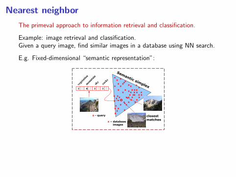
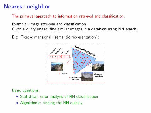
The primeval approach to information retrieval and classification.
Example: image retrieval and classification.Given a query image, find similar images in a database using NN search.
E.g. Fixed-dimensional “semantic representation”:278 From Pixels to Semantic Spaces: Advances in Content-Based Image Search
Fig. 1.7 Query by semantic example. Images are represented as vectors of concept proba-bilities, i.e., points on the semantic probability simplex. The vector computed from a queryimage is compared to those extracted from the images in the database, using a suitable
similarity function. The closest matches are returned by the retrieval system.
Fig. 1.8 Top four matches to the QBSE query derived from the image shown on the left.Because good matches require agreement along various dimensions of the semantic space,QBSE is significantly less prone to the errors made by QBVE. This can be seen by comparing
this set of image matches to those of Figure 1.3.
judgments of similarity that the QBVE matches of that figure.
Inspection of the semantic multinomials associated with all images
shown reveals that, although the query image receives a fair amount
Basic questions:
• Statistical: error analysis of NN classification
• Algorithmic: finding the NN quickly
Nearest neighbor
The primeval approach to information retrieval and classification.
Example: image retrieval and classification.Given a query image, find similar images in a database using NN search.
E.g. Fixed-dimensional “semantic representation”:278 From Pixels to Semantic Spaces: Advances in Content-Based Image Search
Fig. 1.7 Query by semantic example. Images are represented as vectors of concept proba-bilities, i.e., points on the semantic probability simplex. The vector computed from a queryimage is compared to those extracted from the images in the database, using a suitable
similarity function. The closest matches are returned by the retrieval system.
Fig. 1.8 Top four matches to the QBSE query derived from the image shown on the left.Because good matches require agreement along various dimensions of the semantic space,QBSE is significantly less prone to the errors made by QBVE. This can be seen by comparing
this set of image matches to those of Figure 1.3.
judgments of similarity that the QBVE matches of that figure.
Inspection of the semantic multinomials associated with all images
shown reveals that, although the query image receives a fair amount
Basic questions:
• Statistical: error analysis of NN classification
• Algorithmic: finding the NN quickly
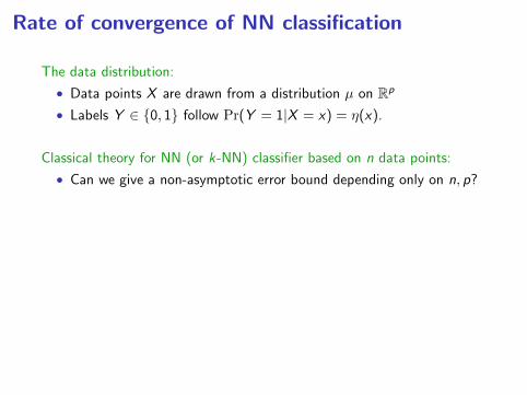
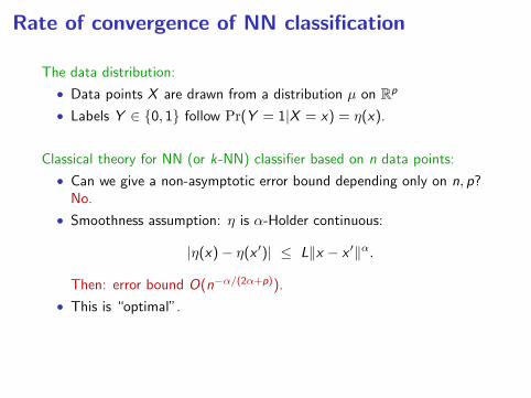
Rate of convergence of NN classification
The data distribution:
• Data points X are drawn from a distribution µ on Rp
• Labels Y ∈ 0, 1 follow Pr(Y = 1|X = x) = η(x).
Classical theory for NN (or k-NN) classifier based on n data points:
• Can we give a non-asymptotic error bound depending only on n, p?
No.
• Smoothness assumption: η is α-Holder continuous:
|η(x)− η(x ′)| ≤ L‖x − x ′‖α.
Then: error bound O(n−α/(2α+p)).
• This is “optimal”.
There exists a distribution with parameter α for which this bound isachieved.
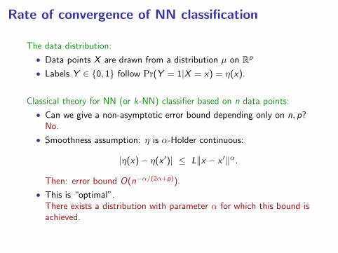
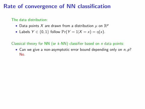
Rate of convergence of NN classification
The data distribution:
• Data points X are drawn from a distribution µ on Rp
• Labels Y ∈ 0, 1 follow Pr(Y = 1|X = x) = η(x).
Classical theory for NN (or k-NN) classifier based on n data points:
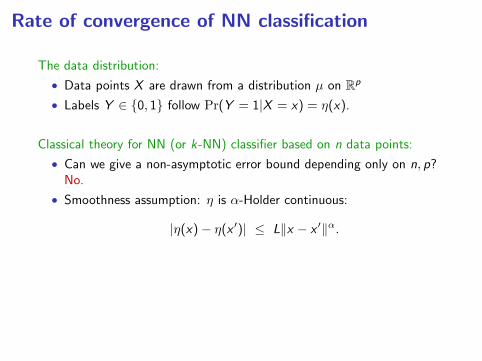
• Can we give a non-asymptotic error bound depending only on n, p?No.
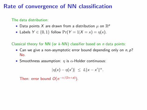
• Smoothness assumption: η is α-Holder continuous:
|η(x)− η(x ′)| ≤ L‖x − x ′‖α.
Then: error bound O(n−α/(2α+p)).
• This is “optimal”.
There exists a distribution with parameter α for which this bound isachieved.
Rate of convergence of NN classification
The data distribution:
• Data points X are drawn from a distribution µ on Rp
• Labels Y ∈ 0, 1 follow Pr(Y = 1|X = x) = η(x).
Classical theory for NN (or k-NN) classifier based on n data points:
• Can we give a non-asymptotic error bound depending only on n, p?No.
• Smoothness assumption: η is α-Holder continuous:
|η(x)− η(x ′)| ≤ L‖x − x ′‖α.
Then: error bound O(n−α/(2α+p)).
• This is “optimal”.There exists a distribution with parameter α for which this bound isachieved.
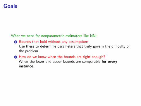
Goals
What we need for nonparametric estimators like NN:
1 Bounds that hold without any assumptions.Use these to determine parameters that truly govern the difficulty ofthe problem.
2 How do we know when the bounds are tight enough?When the lower and upper bounds are comparable for everyinstance.
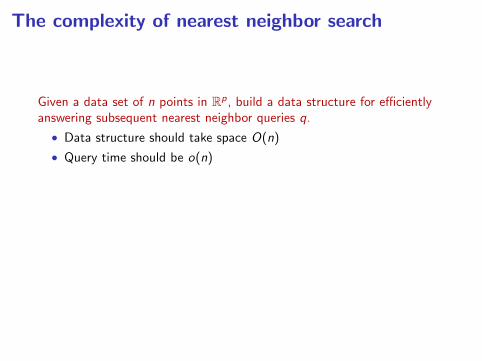
The complexity of nearest neighbor search
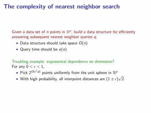
Given a data set of n points in Rp, build a data structure for efficientlyanswering subsequent nearest neighbor queries q.
• Data structure should take space O(n)
• Query time should be o(n)
Troubling example: exponential dependence on dimension?For any 0 < ε < 1,
• Pick 2O(ε2p) points uniformly from the unit sphere in Rp
• With high probability, all interpoint distances are (1± ε)√
2
The complexity of nearest neighbor search
Given a data set of n points in Rp, build a data structure for efficientlyanswering subsequent nearest neighbor queries q.
• Data structure should take space O(n)
• Query time should be o(n)
Troubling example: exponential dependence on dimension?For any 0 < ε < 1,
• Pick 2O(ε2p) points uniformly from the unit sphere in Rp
• With high probability, all interpoint distances are (1± ε)√
2
Approximate nearest neighbor
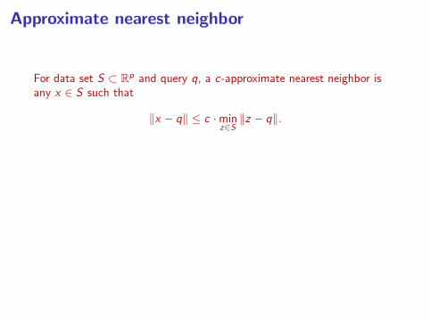
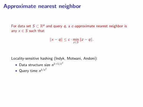
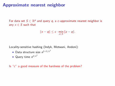
For data set S ⊂ Rp and query q, a c-approximate nearest neighbor isany x ∈ S such that
‖x − q‖ ≤ c ·minz∈S‖z − q‖.
Locality-sensitive hashing (Indyk, Motwani, Andoni):
• Data structure size n1+1/c2
• Query time n1/c2
Is “c” a good measure of the hardness of the problem?
Approximate nearest neighbor
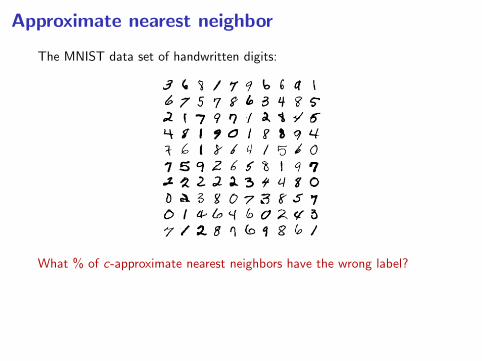
The MNIST data set of handwritten digits:
What % of c-approximate nearest neighbors have the wrong label?
c 1.0 1.2 1.4 1.6 1.8 2.0Error rate (%) 3.1 9.0 18.4 29.3 40.7 51.4
Approximate nearest neighbor
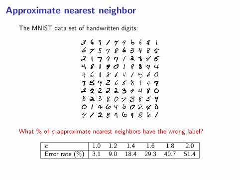
The MNIST data set of handwritten digits:
What % of c-approximate nearest neighbors have the wrong label?
c 1.0 1.2 1.4 1.6 1.8 2.0Error rate (%) 3.1 9.0 18.4 29.3 40.7 51.4

Goals
What we need for nonparametric estimators like NN:
1 Bounds that hold without any assumptions.Use these to determine parameters that truly govern the difficulty ofthe problem.
2 How do we know when the bounds are tight enough?When the lower and upper bounds are comparable for everyinstance.
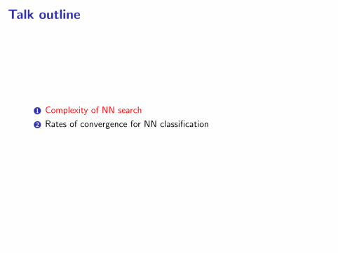
Talk outline
1 Complexity of NN search
2 Rates of convergence for NN classification
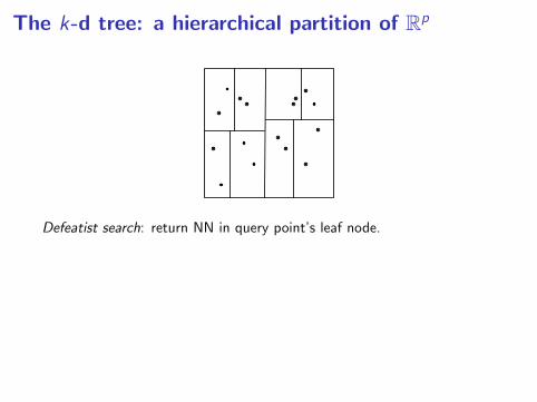
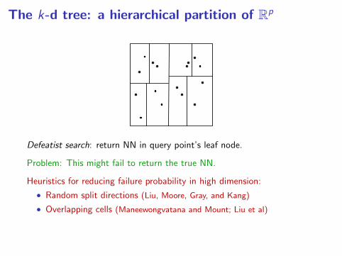
The k-d tree: a hierarchical partition of Rp
Defeatist search: return NN in query point’s leaf node.
Problem: This might fail to return the true NN.
Heuristics for reducing failure probability in high dimension:
• Random split directions (Liu, Moore, Gray, and Kang)
• Overlapping cells (Maneewongvatana and Mount; Liu et al)
Popular option: forests of randomized trees (e.g. FLANN)
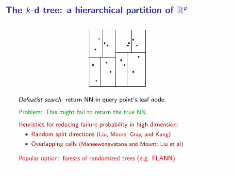
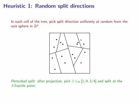
Heuristic 1: Random split directions
In each cell of the tree, pick split direction uniformly at random from theunit sphere in Rp
Perturbed split: after projection, pick β ∈R [1/4, 3/4] and split at theβ-fractile point.
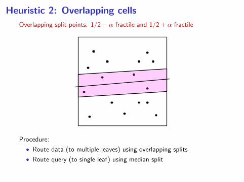
Heuristic 2: Overlapping cells
Overlapping split points: 1/2− α fractile and 1/2 + α fractile
Procedure:
• Route data (to multiple leaves) using overlapping splits
• Route query (to single leaf) using median split
Spill tree has size n1/(1−lg(1+2α)): e.g. n1.159 for α = 0.05.

Heuristic 2: Overlapping cells
Overlapping split points: 1/2− α fractile and 1/2 + α fractile
Procedure:
• Route data (to multiple leaves) using overlapping splits
• Route query (to single leaf) using median split
Spill tree has size n1/(1−lg(1+2α)): e.g. n1.159 for α = 0.05.
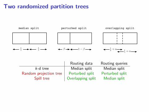
Two randomized partition trees
12 12
1 12 + ↵ 1
2 + ↵
median split perturbed split overlapping split
Routing data Routing queriesk-d tree Median split Median split
Random projection tree Perturbed split Perturbed splitSpill tree Overlapping split Median split
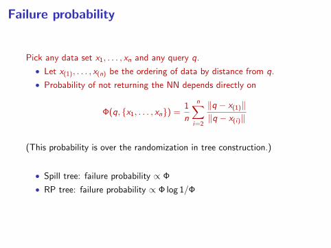
Failure probability
Pick any data set x1, . . . , xn and any query q.
• Let x(1), . . . , x(n) be the ordering of data by distance from q.
• Probability of not returning the NN depends directly on
Φ(q, x1, . . . , xn) =1
n
n∑i=2
‖q − x(1)‖‖q − x(i)‖
(This probability is over the randomization in tree construction.)
• Spill tree: failure probability ∝ Φ
• RP tree: failure probability ∝ Φ log 1/Φ
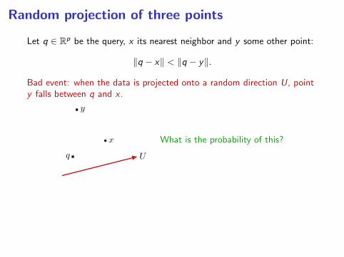
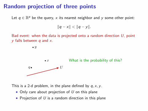
Random projection of three points
Let q ∈ Rp be the query, x its nearest neighbor and y some other point:
‖q − x‖ < ‖q − y‖.
Bad event: when the data is projected onto a random direction U, pointy falls between q and x .
x
y
q U
What is the probability of this?
This is a 2-d problem, in the plane defined by q, x , y .
• Only care about projection of U on this plane
• Projection of U is a random direction in this plane
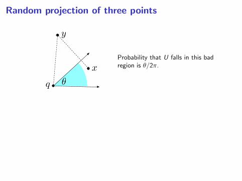
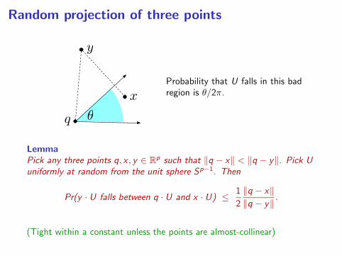
Random projection of three points
x
y
q
Probability that U falls in this badregion is θ/2π.
LemmaPick any three points q, x , y ∈ Rp such that ‖q − x‖ < ‖q − y‖. Pick Uuniformly at random from the unit sphere Sp−1. Then
Pr(y · U falls between q · U and x · U) ≤ 1
2
‖q − x‖‖q − y‖ .
(Tight within a constant unless the points are almost-collinear)
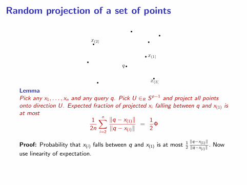
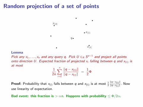
Random projection of a set of points
q
x(2)
x(1)
x(3)
LemmaPick any x1, . . . , xn and any query q. Pick U ∈R Sp−1 and project all pointsonto direction U. Expected fraction of projected xi falling between q and x(1) isat most
1
2n
n∑i=2
‖q − x(1)‖‖q − x(i)‖
=1
2Φ
Proof: Probability that x(i) falls between q and x(1) is at most 12
‖q−x(1)‖‖q−x(i)‖
. Now
use linearity of expectation.
Bad event: this fraction is > αn. Happens with probability ≤ Φ/2α.
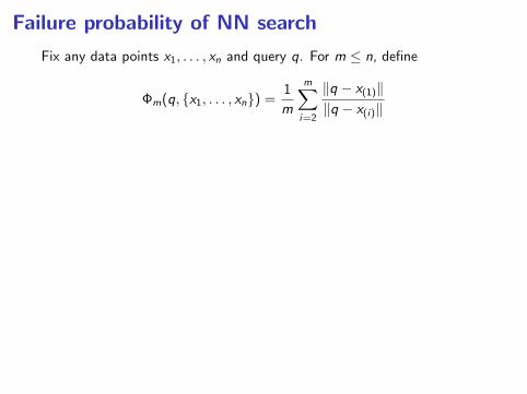
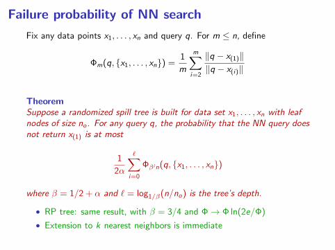
Failure probability of NN search
Fix any data points x1, . . . , xn and query q. For m ≤ n, define
Φm(q, x1, . . . , xn) =1
m
m∑i=2
‖q − x(1)‖‖q − x(i)‖
TheoremSuppose a randomized spill tree is built for data set x1, . . . , xn with leafnodes of size no . For any query q, the probability that the NN query doesnot return x(1) is at most
1
2α
∑i=0
Φβin(q, x1, . . . , xn)
where β = 1/2 + α and ` = log1/β(n/no) is the tree’s depth.
• RP tree: same result, with β = 3/4 and Φ→ Φ ln(2e/Φ)
• Extension to k nearest neighbors is immediate
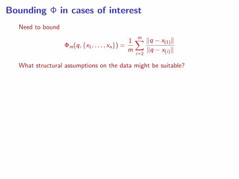
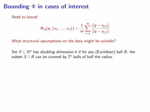
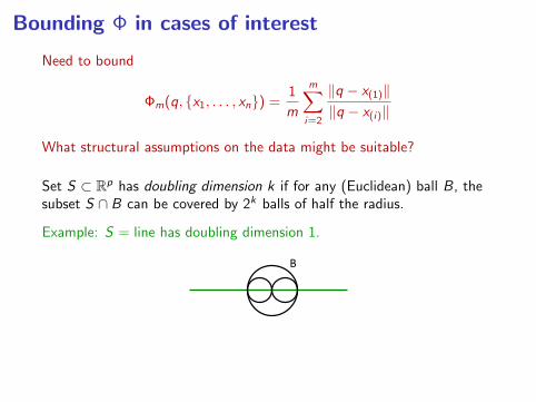
Bounding Φ in cases of interest
Need to bound
Φm(q, x1, . . . , xn) =1
m
m∑i=2
‖q − x(1)‖‖q − x(i)‖
What structural assumptions on the data might be suitable?
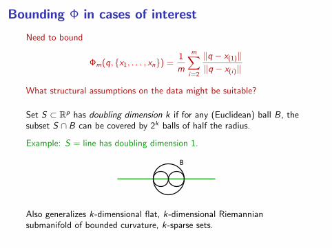
Set S ⊂ Rp has doubling dimension k if for any (Euclidean) ball B, thesubset S ∩ B can be covered by 2k balls of half the radius.
Example: S = line has doubling dimension 1.
Dimension notion #1: doubling dimension
Set S ½ RD has doubling dimension· d if: for any ball B, subset S Å B can be covered by 2d balls of half the radius.
S = lineDoubling dimension = 1
S = k-dimensional affine subspaceDoubling dimension = O(k)
S = set of N pointsDoubling dimension · log N
B S = k-dim submanifold of RD
with finite condition numberDoubling dimension = O(k) in small enough neighborhoods
S = points in RD with at most k nonzero coordinatesDoubling dimension = O(k log D)
Also generalizes k-dimensional flat, k-dimensional Riemanniansubmanifold of bounded curvature, k-sparse sets.
Bounding Φ in cases of interest
Need to bound
Φm(q, x1, . . . , xn) =1
m
m∑i=2
‖q − x(1)‖‖q − x(i)‖
What structural assumptions on the data might be suitable?
Set S ⊂ Rp has doubling dimension k if for any (Euclidean) ball B, thesubset S ∩ B can be covered by 2k balls of half the radius.
Example: S = line has doubling dimension 1.
Dimension notion #1: doubling dimension
Set S ½ RD has doubling dimension· d if: for any ball B, subset S Å B can be covered by 2d balls of half the radius.
S = lineDoubling dimension = 1
S = k-dimensional affine subspaceDoubling dimension = O(k)
S = set of N pointsDoubling dimension · log N
B S = k-dim submanifold of RD
with finite condition numberDoubling dimension = O(k) in small enough neighborhoods
S = points in RD with at most k nonzero coordinatesDoubling dimension = O(k log D)
Also generalizes k-dimensional flat, k-dimensional Riemanniansubmanifold of bounded curvature, k-sparse sets.
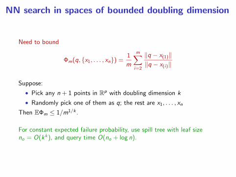
NN search in spaces of bounded doubling dimension
Need to bound
Φm(q, x1, . . . , xn) =1
m
m∑i=2
‖q − x(1)‖‖q − x(i)‖
Suppose:
• Pick any n + 1 points in Rp with doubling dimension k
• Randomly pick one of them as q; the rest are x1, . . . , xn
Then EΦm ≤ 1/m1/k .
For constant expected failure probability, use spill tree with leaf sizeno = O(kk), and query time O(no + log n).
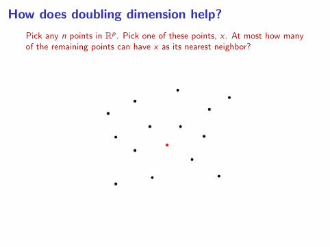
How does doubling dimension help?
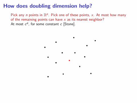
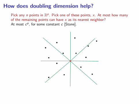
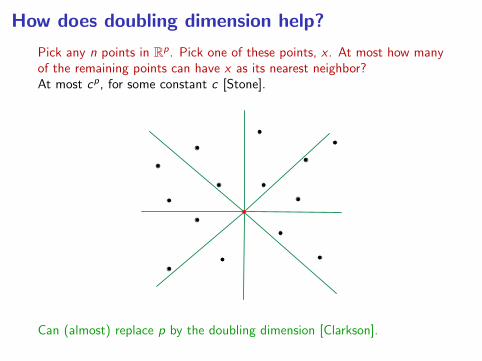
Pick any n points in Rp. Pick one of these points, x . At most how manyof the remaining points can have x as its nearest neighbor?
At most cp, for some constant c [Stone].
Can (almost) replace p by the doubling dimension [Clarkson].
How does doubling dimension help?
Pick any n points in Rp. Pick one of these points, x . At most how manyof the remaining points can have x as its nearest neighbor?At most cp, for some constant c [Stone].
Can (almost) replace p by the doubling dimension [Clarkson].
How does doubling dimension help?
Pick any n points in Rp. Pick one of these points, x . At most how manyof the remaining points can have x as its nearest neighbor?At most cp, for some constant c [Stone].
Can (almost) replace p by the doubling dimension [Clarkson].
How does doubling dimension help?
Pick any n points in Rp. Pick one of these points, x . At most how manyof the remaining points can have x as its nearest neighbor?At most cp, for some constant c [Stone].
Can (almost) replace p by the doubling dimension [Clarkson].
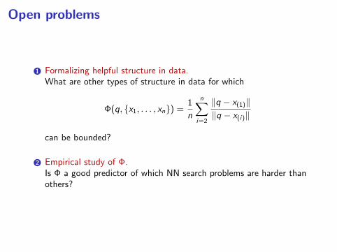
Open problems
1 Formalizing helpful structure in data.What are other types of structure in data for which
Φ(q, x1, . . . , xn) =1
n
n∑i=2
‖q − x(1)‖‖q − x(i)‖
can be bounded?
2 Empirical study of Φ.Is Φ a good predictor of which NN search problems are harder thanothers?
Talk outline
1 Complexity of NN search
2 Rates of convergence for NN classification
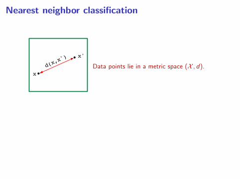
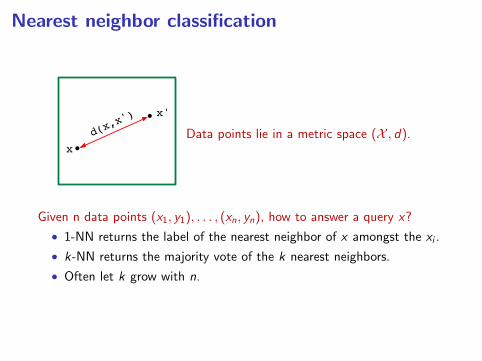
Nearest neighbor classification
x
x'
d(x,x')
Data points lie in a metric space (X , d).
Given n data points (x1, y1), . . . , (xn, yn), how to answer a query x?
• 1-NN returns the label of the nearest neighbor of x amongst the xi .
• k-NN returns the majority vote of the k nearest neighbors.
• Often let k grow with n.
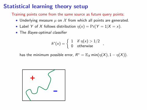
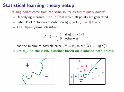
Statistical learning theory setupTraining points come from the same source as future query points:
• Underlying measure µ on X from which all points are generated.
• Label Y of X follows distribution η(x) = Pr(Y = 1|X = x).
• The Bayes-optimal classifier
h∗(x) =
1 if η(x) > 1/20 otherwise
,
has the minimum possible error, R∗ = EX min(η(X ), 1− η(X )).
• Let hn,k be the k-NN classifier based on n labeled data points.
+-
+
-
++
+
+
+
+
-
-- -
--
-
+
++
Questions of interest
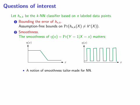
Let hn,k be the k-NN classifier based on n labeled data points.
1 Bounding the error of hn,k .
Assumption-free bounds on Pr(hn,k(X ) 6= h∗(X )).
2 Smoothness.The smoothness of η(x) = Pr(Y = 1|X = x) matters:
x
(x)
x
(x)
• A notion of smoothness tailor-made for NN.• Upper and lower bounds that are qualitatively similar for all
distributions in the same smoothness class.
3 Consistency of NNEarlier work: Universal consistency in Rp [Stone]
Now: Universal consistency in a richer family of metric spaces.
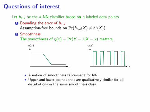
Questions of interest
Let hn,k be the k-NN classifier based on n labeled data points.
1 Bounding the error of hn,k .Assumption-free bounds on Pr(hn,k(X ) 6= h∗(X )).
2 Smoothness.The smoothness of η(x) = Pr(Y = 1|X = x) matters:
x
(x)
x
(x)
• A notion of smoothness tailor-made for NN.• Upper and lower bounds that are qualitatively similar for all
distributions in the same smoothness class.
3 Consistency of NNEarlier work: Universal consistency in Rp [Stone]
Now: Universal consistency in a richer family of metric spaces.
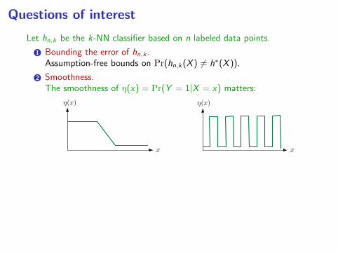
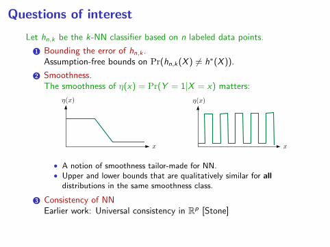
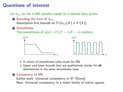
Questions of interest
Let hn,k be the k-NN classifier based on n labeled data points.
1 Bounding the error of hn,k .Assumption-free bounds on Pr(hn,k(X ) 6= h∗(X )).
2 Smoothness.The smoothness of η(x) = Pr(Y = 1|X = x) matters:
x
(x)
x
(x)
• A notion of smoothness tailor-made for NN.
• Upper and lower bounds that are qualitatively similar for alldistributions in the same smoothness class.
3 Consistency of NNEarlier work: Universal consistency in Rp [Stone]
Now: Universal consistency in a richer family of metric spaces.
Questions of interest
Let hn,k be the k-NN classifier based on n labeled data points.
1 Bounding the error of hn,k .Assumption-free bounds on Pr(hn,k(X ) 6= h∗(X )).
2 Smoothness.The smoothness of η(x) = Pr(Y = 1|X = x) matters:
x
(x)
x
(x)
• A notion of smoothness tailor-made for NN.• Upper and lower bounds that are qualitatively similar for all
distributions in the same smoothness class.
3 Consistency of NNEarlier work: Universal consistency in Rp [Stone]
Now: Universal consistency in a richer family of metric spaces.
Questions of interest
Let hn,k be the k-NN classifier based on n labeled data points.
1 Bounding the error of hn,k .Assumption-free bounds on Pr(hn,k(X ) 6= h∗(X )).
2 Smoothness.The smoothness of η(x) = Pr(Y = 1|X = x) matters:
x
(x)
x
(x)
• A notion of smoothness tailor-made for NN.• Upper and lower bounds that are qualitatively similar for all
distributions in the same smoothness class.
3 Consistency of NNEarlier work: Universal consistency in Rp [Stone]Now: Universal consistency in a richer family of metric spaces.
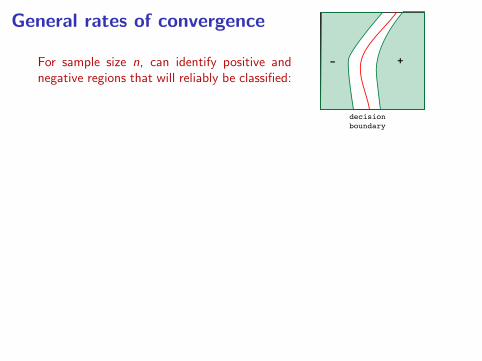
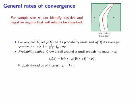
General rates of convergence
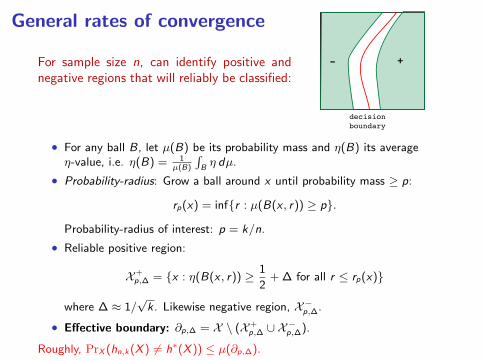
For sample size n, can identify positive andnegative regions that will reliably be classified:
+
decisionboundary
-
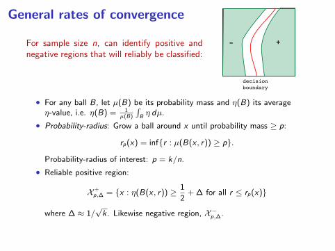
• For any ball B, let µ(B) be its probability mass and η(B) its averageη-value, i.e. η(B) = 1
µ(B)
∫Bη dµ.
• Probability-radius: Grow a ball around x until probability mass ≥ p:
rp(x) = infr : µ(B(x , r)) ≥ p.
Probability-radius of interest: p = k/n.
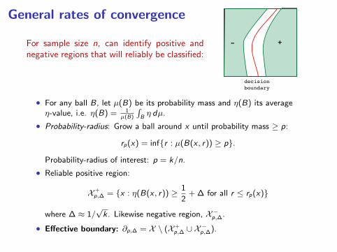
• Reliable positive region:
X+p,∆ = x : η(B(x , r)) ≥ 1
2+ ∆ for all r ≤ rp(x)
where ∆ ≈ 1/√k. Likewise negative region, X−p,∆.
• Effective boundary: ∂p,∆ = X \ (X+p,∆ ∪ X
−p,∆).
Roughly, PrX (hn,k(X ) 6= h∗(X )) ≤ µ(∂p,∆).
General rates of convergence
For sample size n, can identify positive andnegative regions that will reliably be classified:
+
decisionboundary
-
• For any ball B, let µ(B) be its probability mass and η(B) its averageη-value, i.e. η(B) = 1
µ(B)
∫Bη dµ.
• Probability-radius: Grow a ball around x until probability mass ≥ p:
rp(x) = infr : µ(B(x , r)) ≥ p.
Probability-radius of interest: p = k/n.
• Reliable positive region:
X+p,∆ = x : η(B(x , r)) ≥ 1
2+ ∆ for all r ≤ rp(x)
where ∆ ≈ 1/√k. Likewise negative region, X−p,∆.
• Effective boundary: ∂p,∆ = X \ (X+p,∆ ∪ X
−p,∆).
Roughly, PrX (hn,k(X ) 6= h∗(X )) ≤ µ(∂p,∆).
Smoothness and margin conditions
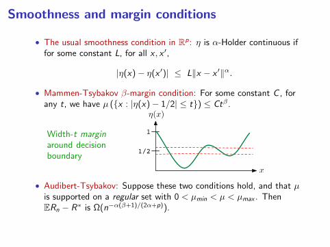
• The usual smoothness condition in Rp: η is α-Holder continuous iffor some constant L, for all x , x ′,
|η(x)− η(x ′)| ≤ L‖x − x ′‖α.
• Mammen-Tsybakov β-margin condition: For some constant C , forany t, we have µ (x : |η(x)− 1/2| ≤ t) ≤ Ctβ .
Width-t marginaround decisionboundary
x
(x)
1/2
1
• Audibert-Tsybakov: Suppose these two conditions hold, and that µis supported on a regular set with 0 < µmin < µ < µmax . ThenERn − R∗ is Ω(n−α(β+1)/(2α+p)).
Under these conditions, for suitable (kn), this rate is achieved by kn-NN.

Smoothness and margin conditions
• The usual smoothness condition in Rp: η is α-Holder continuous iffor some constant L, for all x , x ′,
|η(x)− η(x ′)| ≤ L‖x − x ′‖α.
• Mammen-Tsybakov β-margin condition: For some constant C , forany t, we have µ (x : |η(x)− 1/2| ≤ t) ≤ Ctβ .
Width-t marginaround decisionboundary
x
(x)
1/2
1
• Audibert-Tsybakov: Suppose these two conditions hold, and that µis supported on a regular set with 0 < µmin < µ < µmax . ThenERn − R∗ is Ω(n−α(β+1)/(2α+p)).
Under these conditions, for suitable (kn), this rate is achieved by kn-NN.
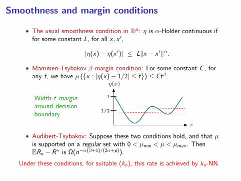
Smoothness and margin conditions
• The usual smoothness condition in Rp: η is α-Holder continuous iffor some constant L, for all x , x ′,
|η(x)− η(x ′)| ≤ L‖x − x ′‖α.
• Mammen-Tsybakov β-margin condition: For some constant C , forany t, we have µ (x : |η(x)− 1/2| ≤ t) ≤ Ctβ .
Width-t marginaround decisionboundary
x
(x)
1/2
1
• Audibert-Tsybakov: Suppose these two conditions hold, and that µis supported on a regular set with 0 < µmin < µ < µmax . ThenERn − R∗ is Ω(n−α(β+1)/(2α+p)).
Under these conditions, for suitable (kn), this rate is achieved by kn-NN.
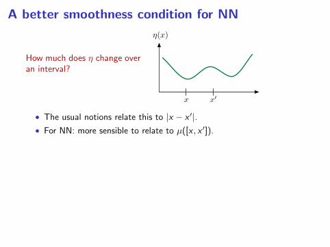
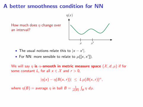
A better smoothness condition for NN
How much does η change overan interval?
(x)
x x0
• The usual notions relate this to |x − x ′|.• For NN: more sensible to relate to µ([x , x ′]).
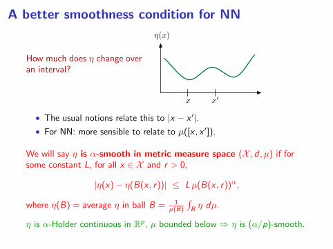
We will say η is α-smooth in metric measure space (X , d , µ) if forsome constant L, for all x ∈ X and r > 0,
|η(x)− η(B(x , r))| ≤ Lµ(B(x , r))α,
where η(B) = average η in ball B = 1µ(B)
∫Bη dµ.
η is α-Holder continuous in Rp, µ bounded below ⇒ η is (α/p)-smooth.
A better smoothness condition for NN
How much does η change overan interval?
(x)
x x0
• The usual notions relate this to |x − x ′|.• For NN: more sensible to relate to µ([x , x ′]).
We will say η is α-smooth in metric measure space (X , d , µ) if forsome constant L, for all x ∈ X and r > 0,
|η(x)− η(B(x , r))| ≤ Lµ(B(x , r))α,
where η(B) = average η in ball B = 1µ(B)
∫Bη dµ.
η is α-Holder continuous in Rp, µ bounded below ⇒ η is (α/p)-smooth.
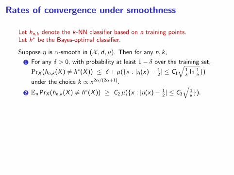
Rates of convergence under smoothness
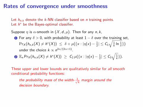
Let hn,k denote the k-NN classifier based on n training points.Let h∗ be the Bayes-optimal classifier.
Suppose η is α-smooth in (X , d , µ). Then for any n, k ,
1 For any δ > 0, with probability at least 1− δ over the training set,
PrX (hn,k(X ) 6= h∗(X )) ≤ δ + µ(x : |η(x)− 12 | ≤ C1
√1k ln 1
δ)under the choice k ∝ n2α/(2α+1).
2 En PrX (hn,k(X ) 6= h∗(X )) ≥ C2 µ(x : |η(x)− 12 | ≤ C3
√1k ).
These upper and lower bounds are qualitatively similar for all smoothconditional probability functions:
the probability mass of the width- 1√k
margin around the
decision boundary.
Rates of convergence under smoothness
Let hn,k denote the k-NN classifier based on n training points.Let h∗ be the Bayes-optimal classifier.
Suppose η is α-smooth in (X , d , µ). Then for any n, k ,
1 For any δ > 0, with probability at least 1− δ over the training set,
PrX (hn,k(X ) 6= h∗(X )) ≤ δ + µ(x : |η(x)− 12 | ≤ C1
√1k ln 1
δ)under the choice k ∝ n2α/(2α+1).
2 En PrX (hn,k(X ) 6= h∗(X )) ≥ C2 µ(x : |η(x)− 12 | ≤ C3
√1k ).
These upper and lower bounds are qualitatively similar for all smoothconditional probability functions:
the probability mass of the width- 1√k
margin around the
decision boundary.
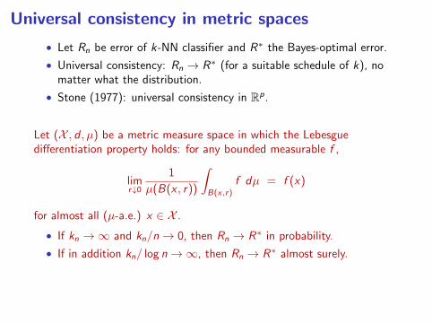
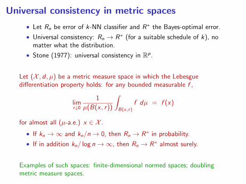
Universal consistency in metric spaces
• Let Rn be error of k-NN classifier and R∗ the Bayes-optimal error.
• Universal consistency: Rn → R∗ (for a suitable schedule of k), nomatter what the distribution.
• Stone (1977): universal consistency in Rp.
Let (X , d , µ) be a metric measure space in which the Lebesguedifferentiation property holds: for any bounded measurable f ,
limr↓0
1
µ(B(x , r))
∫B(x,r)
f dµ = f (x)
for almost all (µ-a.e.) x ∈ X .
• If kn →∞ and kn/n→ 0, then Rn → R∗ in probability.
• If in addition kn/ log n→∞, then Rn → R∗ almost surely.
Examples of such spaces: finite-dimensional normed spaces; doublingmetric measure spaces.
Open problems
1 Are there metric spaces in which k-NN fails to be consistent?
2 Consistency in more general distance spaces.
Open problems
1 Are there metric spaces in which k-NN fails to be consistent?
2 Consistency in more general distance spaces.