distributed optimization with its applications to …
TRANSCRIPT

DISTRIBUTED OPTIMIZATION WITH
ITS APPLICATIONS TO POWER
SYSTEMS
A THESIS SUBMITTED TO THE UNIVERSITY OF MANCHESTER
FOR THE DEGREE OF DOCTOR OF PHILOSOPHY
IN THE FACULTY OF SCIENCE & ENGINEERING
2019
Tianqiao Zhao
School of Electrical and Electronic Engineering

Contents
List of Figures 9
Symbols 13
Abbreviations 15
Abstract 17
Declaration 18
Copyright Statement 19
Publications 20
Acknowledgements 22
1 Introduction 24
1.1 Overview of Modern Power Systems . . . . . . . . . . . . . . . . . . . . . 24
1.1.1 Microgrids . . . . . . . . . . . . . . . . . . . . . . . . . . . . . . 26
1.1.2 Distributed Generation . . . . . . . . . . . . . . . . . . . . . . . . 26
2

1.1.3 Energy Storage System . . . . . . . . . . . . . . . . . . . . . . . . 27
1.1.4 Plug-in Electric Vehicles . . . . . . . . . . . . . . . . . . . . . . . 27
1.2 Research Scope . . . . . . . . . . . . . . . . . . . . . . . . . . . . . . . . 27
1.3 Contributions . . . . . . . . . . . . . . . . . . . . . . . . . . . . . . . . . 29
1.4 Thesis Outline . . . . . . . . . . . . . . . . . . . . . . . . . . . . . . . . . 31
1.5 Summary . . . . . . . . . . . . . . . . . . . . . . . . . . . . . . . . . . . 33
2 Preliminaries 34
2.1 Notation . . . . . . . . . . . . . . . . . . . . . . . . . . . . . . . . . . . . 34
2.1.1 Graph Theory . . . . . . . . . . . . . . . . . . . . . . . . . . . . . 34
2.1.2 Nonsmooth Analysis and Differential Inclusions . . . . . . . . . . 35
2.2 Saddle Points . . . . . . . . . . . . . . . . . . . . . . . . . . . . . . . . . 36
3 Literature Review: Economic Operation in Microgrids 37
3.1 Introduction . . . . . . . . . . . . . . . . . . . . . . . . . . . . . . . . . . 37
3.2 Overview of Multi-agent Systems . . . . . . . . . . . . . . . . . . . . . . 37
3.2.1 Multi-agent Systems in Modern Power Systems . . . . . . . . . . . 38
3.3 Economic Operation in Microgrids . . . . . . . . . . . . . . . . . . . . . . 38
3.3.1 PEVs Charging Management . . . . . . . . . . . . . . . . . . . . . 39
3.3.2 Energy Management System for Microgrids . . . . . . . . . . . . . 40
3.3.3 Energy Management System for Multiple Battery Energy Storage
Systems . . . . . . . . . . . . . . . . . . . . . . . . . . . . . . . . 43
3

3.4 Summary . . . . . . . . . . . . . . . . . . . . . . . . . . . . . . . . . . . 44
4 Distributed Initialization-Free Cost-Optimal Charging Control of Plug-in Elec-
tric Vehicles 45
4.1 Introduction . . . . . . . . . . . . . . . . . . . . . . . . . . . . . . . . . . 45
4.2 Problem Formulation for the Battery Charging Problem of PEVs . . . . . . 46
4.2.1 Battery Modelling . . . . . . . . . . . . . . . . . . . . . . . . . . 46
4.2.2 Constraints . . . . . . . . . . . . . . . . . . . . . . . . . . . . . . 47
4.2.3 Optimization Problem Formulation of PEVs . . . . . . . . . . . . . 48
4.3 Distributed Optimal Solution . . . . . . . . . . . . . . . . . . . . . . . . . 51
4.3.1 Problem Reformulation . . . . . . . . . . . . . . . . . . . . . . . . 51
4.3.2 Distributed Algorithmic Design . . . . . . . . . . . . . . . . . . . 52
4.3.3 Convergence Analysis . . . . . . . . . . . . . . . . . . . . . . . . 53
4.4 Simulation Results and Analysis . . . . . . . . . . . . . . . . . . . . . . . 56
4.4.1 Algorithm Implementation . . . . . . . . . . . . . . . . . . . . . . 57
4.4.2 Simulation Studies . . . . . . . . . . . . . . . . . . . . . . . . . . 58
4.5 Conclusion . . . . . . . . . . . . . . . . . . . . . . . . . . . . . . . . . . 67
5 Distributed Agent Consensus-Based Optimal Resource Management for Micro-
grids 68
5.1 Introduction . . . . . . . . . . . . . . . . . . . . . . . . . . . . . . . . . . 68
5.2 Problem Formulation . . . . . . . . . . . . . . . . . . . . . . . . . . . . . 69
5.2.1 Constraints . . . . . . . . . . . . . . . . . . . . . . . . . . . . . . 70
4

5.2.2 Objective Function . . . . . . . . . . . . . . . . . . . . . . . . . . 71
5.3 Distributed solution of dynamic economic dispatch . . . . . . . . . . . . . 71
5.3.1 Distributed Algorithm Design . . . . . . . . . . . . . . . . . . . . 72
5.3.2 Convergence Analysis . . . . . . . . . . . . . . . . . . . . . . . . 73
5.4 Simulation Results and Analysis . . . . . . . . . . . . . . . . . . . . . . . 77
5.4.1 Case 5.1 . . . . . . . . . . . . . . . . . . . . . . . . . . . . . . . . 79
5.4.2 Case 5.2 . . . . . . . . . . . . . . . . . . . . . . . . . . . . . . . . 80
5.4.3 Case 5.3 . . . . . . . . . . . . . . . . . . . . . . . . . . . . . . . . 84
5.5 Conclusion . . . . . . . . . . . . . . . . . . . . . . . . . . . . . . . . . . 85
6 Distributed Finite-Time Optimal Resource Management for Microgrids Based
on Multi-Agent Framework 87
6.1 Introduction . . . . . . . . . . . . . . . . . . . . . . . . . . . . . . . . . . 87
6.2 Multi-agent System Architecture of a Microgrid . . . . . . . . . . . . . . . 88
6.2.1 Multi-agent System Framework . . . . . . . . . . . . . . . . . . . 88
6.2.2 The Agent Description under MAS Framework . . . . . . . . . . . 88
6.3 Finite-time Distributed Optimal Solution for the Islanded Microgrid . . . . 91
6.3.1 Alternative Formulation . . . . . . . . . . . . . . . . . . . . . . . 92
6.3.2 Finite-time Distributed Optimal Energy Management . . . . . . . . 93
6.4 Finite-time Distributed Solution for Grid-connected Microgrid . . . . . . . 96
6.5 Simulation Results and Analysis . . . . . . . . . . . . . . . . . . . . . . . 98
6.5.1 Case 6.1 . . . . . . . . . . . . . . . . . . . . . . . . . . . . . . . . 100
5

6.5.2 Case 6.2 . . . . . . . . . . . . . . . . . . . . . . . . . . . . . . . . 101
6.5.3 Case 6.3 . . . . . . . . . . . . . . . . . . . . . . . . . . . . . . . . 104
6.5.4 Case 6.4 . . . . . . . . . . . . . . . . . . . . . . . . . . . . . . . . 105
6.6 Conclusion . . . . . . . . . . . . . . . . . . . . . . . . . . . . . . . . . . 105
7 Consensus-Based Distributed Fixed-time Economic Dispatch under Uncertain
Information in Microgrids 109
7.1 Problem Formulation . . . . . . . . . . . . . . . . . . . . . . . . . . . . . 109
7.1.1 Objective Function in the Microgrid . . . . . . . . . . . . . . . . . 109
7.2 Distributed Fixed-time Energy Management System under Uncertainty . . . 112
7.2.1 Algorithm Design . . . . . . . . . . . . . . . . . . . . . . . . . . 113
7.3 Simulation Study . . . . . . . . . . . . . . . . . . . . . . . . . . . . . . . 118
7.3.1 Parameter Setup . . . . . . . . . . . . . . . . . . . . . . . . . . . 118
7.3.2 Algorithm Implementation with Local Constraints . . . . . . . . . 119
7.3.3 Case 7.1 . . . . . . . . . . . . . . . . . . . . . . . . . . . . . . . . 119
7.3.4 Case 7.2 . . . . . . . . . . . . . . . . . . . . . . . . . . . . . . . . 122
7.3.5 Case 7.3 . . . . . . . . . . . . . . . . . . . . . . . . . . . . . . . . 123
7.4 Conclusion . . . . . . . . . . . . . . . . . . . . . . . . . . . . . . . . . . 126
8 Cooperative Optimal Control of Battery Energy Storage System under Wind
Uncertainties in a Microgrid 127
8.1 Introduction . . . . . . . . . . . . . . . . . . . . . . . . . . . . . . . . . . 127
8.2 Network Model of Multiple Battery Energy Storage Systems . . . . . . . . 128
6

8.2.1 Overview of Multiple Battery Energy Storage Systems . . . . . . . 128
8.3 Distributed Energy Management of Battery Energy Storage Systems under
Wind Power uncertainties . . . . . . . . . . . . . . . . . . . . . . . . . . . 129
8.4 Consensus-based Cooperative Algorithm Design . . . . . . . . . . . . . . 131
8.4.1 Solution Set of Distributed Energy Management . . . . . . . . . . 132
8.4.2 Distributed Cooperative Algorithm Design . . . . . . . . . . . . . 132
8.4.3 Convergence Analysis . . . . . . . . . . . . . . . . . . . . . . . . 134
8.4.4 The Coordination of BESSs under Wind Power Generation Error . . 135
8.4.5 Algorithm Implementation . . . . . . . . . . . . . . . . . . . . . . 136
8.5 Simulation Results and analysis . . . . . . . . . . . . . . . . . . . . . . . 136
8.5.1 Case 8.1 . . . . . . . . . . . . . . . . . . . . . . . . . . . . . . . . 138
8.5.2 Case 8.2 . . . . . . . . . . . . . . . . . . . . . . . . . . . . . . . . 139
8.5.3 Case 8.3 . . . . . . . . . . . . . . . . . . . . . . . . . . . . . . . . 143
8.5.4 Case 8.4 . . . . . . . . . . . . . . . . . . . . . . . . . . . . . . . . 143
8.6 Conclusion . . . . . . . . . . . . . . . . . . . . . . . . . . . . . . . . . . 147
9 Future Works 148
9.1 Future Research . . . . . . . . . . . . . . . . . . . . . . . . . . . . . . . . 148
Bibliography 150
A Data for Test Systems 167
A.1 Line Data for IEEE 14-bus System . . . . . . . . . . . . . . . . . . . . . . 167
7

A.2 Line Data for IEEE 30-bus System . . . . . . . . . . . . . . . . . . . . . . 168
8

List of Figures
1.1 The conceptual model of a smart grid [1] . . . . . . . . . . . . . . . . . . . 25
1.2 Outlines of research scope . . . . . . . . . . . . . . . . . . . . . . . . . . 28
3.1 A diagram of the RG and parallel-connected ESS . . . . . . . . . . . . . . 41
4.1 The simple equivalent circuit model . . . . . . . . . . . . . . . . . . . . . 47
4.2 Distributed demand management for PEVs charging . . . . . . . . . . . . . 57
4.3 The general operation structure of ith agent . . . . . . . . . . . . . . . . . 59
4.4 The communication topology for PEVs charging . . . . . . . . . . . . . . 60
4.5 The charging power updates for PEVs . . . . . . . . . . . . . . . . . . . . 60
4.6 Total allocated charging power updates for PEVs . . . . . . . . . . . . . . 61
4.7 Allocated charging power updates for PEVs . . . . . . . . . . . . . . . . . 61
4.8 Supply-demand mismatch updates for PEVs . . . . . . . . . . . . . . . . . 62
4.9 The SoC updates for PEVs . . . . . . . . . . . . . . . . . . . . . . . . . . 62
4.10 Allocated charging power updates for PEVs . . . . . . . . . . . . . . . . . 64
4.11 Supply-demand mismatch updates for PEVs . . . . . . . . . . . . . . . . . 64
4.12 Allocated charging power updates for 30-PEVs . . . . . . . . . . . . . . . 65
9

4.13 Supply-demand mismatch updates for 30-PEVs . . . . . . . . . . . . . . . 66
4.14 Allocated charging power updates for 60-PEVs . . . . . . . . . . . . . . . 66
4.15 Supply-demand mismatch updates for 60-PEVs . . . . . . . . . . . . . . . 67
5.1 General operation diagram of an agent. . . . . . . . . . . . . . . . . . . . . 77
5.2 IEEE 14-bus system. . . . . . . . . . . . . . . . . . . . . . . . . . . . . . 78
5.3 The actual output power of RGs and ESSs . . . . . . . . . . . . . . . . . . 80
5.4 The supply-demand mismatch update . . . . . . . . . . . . . . . . . . . . 81
5.5 The actual output power of RGs and ESSs . . . . . . . . . . . . . . . . . . 81
5.6 The supply-demand mismatch update . . . . . . . . . . . . . . . . . . . . 82
5.7 The actual output power of RGs and ESSs during the single link failure . . 82
5.8 The supply-demand mismatch update . . . . . . . . . . . . . . . . . . . . 83
5.9 Total allocated output power . . . . . . . . . . . . . . . . . . . . . . . . . 83
5.10 The actual output power of RGs and ESSs during the single node failure . . 84
5.11 The supply-demand mismatch update . . . . . . . . . . . . . . . . . . . . 85
5.12 The actual power output of RGs and ESSs . . . . . . . . . . . . . . . . . . 86
5.13 The supply-demand mismatch update . . . . . . . . . . . . . . . . . . . . 86
6.1 The communication network of agents in a microgrid . . . . . . . . . . . . 89
6.2 IEEE 14-bus system . . . . . . . . . . . . . . . . . . . . . . . . . . . . . . 99
6.3 The marginal cost update with the proposed finite-time algorithm . . . . . . 101
6.4 The marginal cost update with the distributed gradient algorithm . . . . . . 102
10

6.5 The marginal cost update with the Laplacian-gradient dynamics . . . . . . 102
6.6 The marginal cost update with the proposed finite-time algorithm . . . . . . 103
6.7 The actual output power . . . . . . . . . . . . . . . . . . . . . . . . . . . 103
6.8 An actual islanded system in China [2] . . . . . . . . . . . . . . . . . . . . 105
6.9 The marginal cost update with the proposed finite-time algorithm for an
actual islanded microgrid . . . . . . . . . . . . . . . . . . . . . . . . . . . 106
6.10 The actual output power . . . . . . . . . . . . . . . . . . . . . . . . . . . 106
6.11 The marginal cost update . . . . . . . . . . . . . . . . . . . . . . . . . . . 107
6.12 The actual output power . . . . . . . . . . . . . . . . . . . . . . . . . . . 107
7.1 The incremental cost of participants . . . . . . . . . . . . . . . . . . . . . 121
7.2 The active power updates of participants . . . . . . . . . . . . . . . . . . . 121
7.3 The total active power of participants . . . . . . . . . . . . . . . . . . . . . 121
7.4 The incremental cost of participants under plug-and-play operation . . . . . 122
7.5 The active power updates of participants under plug-and-play operation . . 122
7.6 The total active power of participants under plug-and-play operation . . . . 123
7.7 The incremental cost under curtailments of renewable generation . . . . . . 124
7.8 The active power update under curtailments of renewable generation . . . . 124
7.9 The total active power under curtailments of renewable generation . . . . . 124
7.10 The incremental cost under varying demand . . . . . . . . . . . . . . . . . 125
7.11 The active power update under varying demand . . . . . . . . . . . . . . . 125
7.12 The total active power under varying demand . . . . . . . . . . . . . . . . 125
11

8.1 Multiple BESSs System . . . . . . . . . . . . . . . . . . . . . . . . . . . . 128
8.2 Coordination scheme of wind generation and BESSs . . . . . . . . . . . . 137
8.3 The control diagram for a BESS . . . . . . . . . . . . . . . . . . . . . . . 138
8.4 The time of use tariff . . . . . . . . . . . . . . . . . . . . . . . . . . . . . 139
8.5 The marginal cost update under the proposed algorithm . . . . . . . . . . . 140
8.6 The marginal cost update under the algorithm in [3] . . . . . . . . . . . . . 140
8.7 The marginal cost update under the proposed algorithm . . . . . . . . . . . 141
8.8 The output power update under the proposed algorithm . . . . . . . . . . . 141
8.9 The power balance estimation . . . . . . . . . . . . . . . . . . . . . . . . 142
8.10 The total output power of BESSs . . . . . . . . . . . . . . . . . . . . . . . 142
8.11 The output power profile of the wind power generation . . . . . . . . . . . 143
8.12 The output power update under the proposed algorithm . . . . . . . . . . . 144
8.13 The power balance estimation . . . . . . . . . . . . . . . . . . . . . . . . 144
8.14 Single line diagram of the 30-BESS system . . . . . . . . . . . . . . . . . 145
8.15 The output power update under the proposed algorithm . . . . . . . . . . . 146
8.16 The power balance estimation . . . . . . . . . . . . . . . . . . . . . . . . 146
12

Symbols
λ(·) The eigenvalue of a marix
λ2 (·) The smallest non-zero eigenvalue of (·)
[·]+ The projection operator on the non-negative real number
A The adjacency matrix of the graph
E The edge set of a graph
G A graph
L The Laplacian matrix
V The node set of a graph
‖·‖ The l2 Euclidean norm of a matrix or a vector
∂ f (·) The partial derivative of a function f (·) with respect to a variable x
O f (·) The gradient of a function f (·)
AT The transpose of a matrix or a vector A
ai agent i chosen control action
ai j The entry in the ith row and jth column of a matrix A
C (·) Cost function
diag(·) diagonal matrix
L The operation of Lie derivative
13

Pi Active power from ith agent
U (·) Utility function
vi ith node
14

Abbreviations
BESSs Battery Energy Storage Systems.
CG Conventional Generators.
DER Distributed Energy Resource.
DG Distributed Generator.
DGA Distributed Gradient Algorithm.
DoD Depth of Discharging.
EGD Economic Generation Dispatch.
EMS Energy Management Systems.
ESS Energy storage system.
EV Electric Vehicle.
ICE Internal Combustion Engine.
ISS Input-to-State Stability.
KKT KarushKuhnTucker.
LGD Laplacian-Gradient Dynamics.
MAS Multi-agent Systems.
MPPT Maximum Peak Power Tracking.
15

PCC Point of Common Coupling.
PEV Plug-in Electrical Vehicle.
PMS Power Management System.
PV Photovoltaic.
RG Renewable Generator.
RTP Real-time Price.
SG Synchronous Generator.
SoC State of Charge.
SSC Storage System Controller.
ToU Time-of-Use.
V2G Vehicle-to-Grid.
WT Wind Turbine.
16

The University of Manchester
Tianqiao Zhao
Doctor of Philosophy
Distributed Optimization with Its Applications to Power Systems
March 13, 2019
The traditional electric power grid is in the process of being transformed from the con-
ventional power grid to an intelligent grid, a so-called smart grid. The operation of smart
grids no longer has one-directional energy and information flow, and enables communica-
tion between utilities and consumers, which is a potential solution to motivating end users to
participate in the decision-making of a demand response. The traditional solution for energy
management problems is a centralized algorithm, which requires a control centre to collect
and process the algorithm. However, it could lose its effectiveness due to the increasing
level of distributed energy resources (DERs). The distributed method is a potential solution
to the problem caused by the centralized method.
The research in this thesis mainly focuses on the feasibility of improving the energy man-
agement system (EMS) of smart grids from the demand side to the supply side. First, a
coordination strategy of the plug-in electric vehicle (PEV) charging process is studied by
maximizing the welfare and satisfaction of PEV owners.It is a distributed algorithm and
analysis shows that it solves the optimal charging problem in an initialization-free approach.
Second, the resource management of renewable generators (RGs) and energy storage sys-
tems (ESSs) is investigated. The objective is to minimize the curtailment of renewable
energy, and at the same time, to minimize the power losses of ESSs. An optimal solution
is proposed to the management problem by enhancing the communication and coordination
under a multi-agent system (MAS) framework. Third, from the above research, it is found
that the operation of microgrids may change frequently and without warning. A distributed
finite-time algorithm is designed for EMSs in a microgrid under different operation modes.
Fourth, a novel fixed-time distributed solution is introduced that both achieves a fast conver-
gence speed and is robust to dealing with uncertain information. Finally, a novel distributed
strategy for multiple BESSs is proposed for optimally coordinating them under uncertainties
of wind power generation while considering the privacy of users.
17

Declaration
No portion of the work referred to in this thesis has been submitted in support of an appli-
cation for another degree or qualification of this or any other university or other institute of
learning.
18

Copyright Statement
i. The author of this thesis (including any appendices and/or schedules to this thesis) owns
certain copyright or related rights in it (the “Copyright”) and s/he has given The University
of Manchester certain rights to use such Copyright, including for administrative purposes.
ii. Copies of this thesis, either in full or in extracts and whether in hard or electronic copy,
may be made only in accordance with the Copyright, Designs and Patents Act 1988 (as
amended) and regulations issued under it or, where appropriate, in accordance with li-
censing agreements which the University has from time to time. This page must form
part of any such copies made.
iii. The ownership of certain Copyright, patents, designs, trade marks and other intellectual
property (the “Intellectual Property”) and any reproductions of copyright works in the
thesis, for example graphs and tables (“Reproductions”), which may be described in this
thesis, may not be owned by the author and may be owned by third parties. Such Intellec-
tual Property and Reproductions cannot and must not be made available for use without
the prior written permission of the owner(s) of the relevant Intellectual Property and/or
Reproductions.
iv. Further information on the conditions under which disclosure, publication and com-
mercialisation of this thesis, the Copyright and any Intellectual Property and/or Repro-
ductions described in it may take place is available in the University IP Policy (see
http://documents.manchester.ac.uk/DocuInfo.aspx?DocID=487), in any relevant Thesis
restriction declarations deposited in the University Library, The University Library’s reg-
ulations (see http://www.manchester.ac.uk/library/aboutus/regulations) and in The Uni-
versity’s Policy on Presentation of Theses.
19

Publications
Journal papers:
1). Tianqiao Zhao and Zhengtao Ding, ’Distributed initialization-free cost-optimal charging
control of plug-in electric vehicles for demand management’ IEEE Transactions on In-
dustrial Informatics, vol. 13, no. 6, pp. 2791-2801, Dec. 2017.
2). Tianqiao Zhao and Zhengtao Ding, ’Distributed Agent Consensus-Based Optimal Re-
source Management for Microgrids’ IEEE Transactions on Sustainable Energy, vol. 9,
no. 1, pp. 443-452, Jan. 2018.
3). Tianqiao Zhao and Zhengtao Ding, ’Distributed Finite-Time Optimal Resource Manage-
ment for Microgrids Based on Multi-Agent Framework’ IEEE Transactions on Industrial
Electronics, vol. 65, no. 8, pp. 6571-6580, Aug. 2018.
4). Tianqiao Zhao and Zhengtao Ding, ’Cooperative Optimal Control of Battery Energy Stor-
age System under Wind Uncertainties in a Microgrid’ IEEE Transactions on Power Sys-
tems, vol. 33, no. 2, pp. 2292-2300, March 2018.
5). Tianqiao Zhao, Zhenhong Li and Zhengtao Ding, ’Consensus-based Distributed Optimal
Energy Management with Less Communication in a Microgrid’ IEEE Transactions on
Industrial Informatics (in press), September 2018.
6). Tianqiao Zhao and Zhengtao Ding, ’Consensus-Based Distributed Fixed-time Economic
Dispatch under Uncertain Information in Microgrids’ submitted to IEEE Transactions on
Control System Technology.
20

7). Tianqiao Zhao and Zhengtao Ding, ’A Distributed Optimal Management System for Co-
ordinating the Generation Side and Demand Side Simultaneously’ submitted to IET Gen-
eration, Transmission & Distribution
Conference papers
1). Tianqiao Zhao, Zongyu Zuo, and Zhengtao Ding, 2017, ’ Cooperative control of dis-
tributed battery energy storage systems in Microgrids ’ in preceding of 2016 35th Chinese
Control Conference (CCC), Chengdu, 2016, pp. 10019-10024.
2). Tianqiao Zhao and Zhengtao Ding, 2017, ’Optimal Energy Management of Microgrid via
Distributed Primal-Dual Dynamics for Fast Frequency Recovery’ in preceding of 2017
IEEE Power & Energy Society General Meeting, Chicago, IL, 2017, pp. 1-5.
21

Acknowledgements
It is a pleasure to acknowledge my appreciation to the people who have made this thesis
possible. I am so excited to reach the completion of my PhD research program which was
an important career and life milestone. I would like to thank all the people who have been
helping me in the successful completion of my PhD research program.
First and foremost, I would like to offer my deepest and sincere gratitude to my supervisor,
Professor Zhengtao Ding for his supervision in these years. He led me through the door
of cooperative control and optimization, and pointed out the new research field to form my
PhD project. Without his advice and support, the research presented in this thesis would not
have been possible.
I would also like to say thank you to all Control Systems Centre colleagues who helped me
to solve the difficulties that I encountered during my studies.
I owe my deepest gratitude to my parents and my wife, who have provided me with uncondi-
tional love, support, and understanding throughout my life and especially through my Ph.D
study. Last but not least, I would like to thank all those whose names I may have missed out
but who have joined me in some way on my research journey.
22

To My Loving Parents and Wife
23

Chapter 1
Introduction
1.1 Overview of Modern Power Systems
The traditional electric power grid is in the process of being transformed from the conven-
tional power grid to an intelligent grid due to the growing demand for electrical energy
from consumers, the integrated need for renewable energy resources, and the transforma-
tion of ageing power grid infrastructures. The future grid [4] is a so-called smart grid that is
an aggregation of distributed generation units, responsive demands, and storage units each
equipped with controllable power electronics devices connected to each other through com-
munication networks [5, 6].
The traditional power grid is centralized and has one-directional energy and information
flow. In contrast, as shown in Fig. 1.1, a smart grid is characterized by the bi-directional flow
of energy and information, and enables communication between utilities and consumers,
which is a potential solution to motivating end users to participate in the decision-making of
demand response. The following goals and characteristics are defined by the Energy Inde-
pendence and Security Act of 2007 (EISA), TitleXIII and National Institute of Technology
(NIST) [7]. First, a smart grid requires the dynamic optimization of grid operations and re-
sources with full cyber-security; second, it should deploy and integrate distributed resources
24

CHAPTER 1. INTRODUCTION 25
Figure 1.1: The conceptual model of a smart grid [1]
and generation, including renewable resources; third, demand response, demand-side re-
sources, and energy-efficiency resources should be incorporated and developed; lastly, ad-
vanced electricity storage and peak-shaving technologies, including plug-in electric and hy-
brid electric vehicles, and thermal-storage air conditioning should be deployed and inte-
grated into smart grids.
These goals cannot be achieved without advanced control and optimization technologies.
Considering the number and variety of distributed controllable devices, managing a smart
grid requires a new paradigm shift in centralized EMS, which needs to consider the local in-
telligence of the distributed units and their communication capability [8]. Such units in Fig.
1.1 are able to sense their local environment, perform local computations, and coordinate
with their neighbours through local communications. These elements play an important role
in improving the flexibility and energy efficiency of smart grids.

CHAPTER 1. INTRODUCTION 26
1.1.1 Microgrids
The conception of the microgrid is a key component of smart grids. Generally, variously
distributed generators (DGs) comprising wind turbines (WTs) and photovoltaic (PV) gen-
erators, energy storage systems (ESSs), loads and other devices are integrated into a micro-
grid to support a flexible and efficient electric network [9]. It can help to integrate these
low-carbon devices into the traditional power grid to enhance the reliability and reduce the
carbon emission. Furthermore, its structure is fundamental in supporting increasing pen-
etration of PEVs. On the one hand, the microgrid is a small-scale power system that can
achieve the power dispatch and supply-demand balance economically within the microgrid
because of the function of advanced EMSs. The EMS play a significant role in the control
of a microgrid, which is able to optimally dispatch the active power of controllable DERs
and control the consumption of controllable loads, subject to certain economic criteria. On
the other hand, a microgrid can be treated as a ’virtual’ power source or load. Through
the coordinated control of the output power of distributed generation within the microgrid,
the peak-shifting or load shaving can be realized, thus reducing the impact of intermittent
renewable generation on main grids or users. A microgrid is usually operated in the grid-
connected mode, which exchanges power with the main grid through the point of common
coupling (PCC) [10, 11]. Due to planned or unexpected reasons [12], the microgrid will be
operated in the islanded mode that needs to maintain its own active power supply-demand
balance. However, because of the intermittency of WTs and PVs, a microgrid has to face
new operational and control challenges of resource management, especially in the islanded
operation mode.
1.1.2 Distributed Generation
Generally, distributed generation includes combined heat and power (CHP), fuel cells, micro-
turbines, photovoltaic systems, wind turbines and hydroelectric energy, etc., and is intended
to be the main backup supplier of energy for improving the reliability in a microgrid. Due
to the flexibility and low-carbon feature of DERs, they can be installed sufficiently close to
energy consumers. As a result, the transmitting electricity loss could be reduced compared
to conventional power systems. However, due to their non-dispatchable feature, they are

CHAPTER 1. INTRODUCTION 27
complemented by controllable generators such as diesel generators, and ESSs.
1.1.3 Energy Storage System
Distributed ESSs are referred to as devices that can absorb excessive power and compensate
for insufficient power during peak generation and load periods. Furthermore, the system
frequency in the low-inertia microgrid may change rapidly due to the increasing high pen-
etration of intermittent renewable generation. Distributed ESSs are power electronic-based
components and thus have a faster response time. Therefore, they are an ideal supplement
for intermittent distributed renewable generation, such as solar power and wind power gen-
eration, since they can store excess energy and rapidly feed it back when needed to minimize
the active power imbalance of an islanded microgrid.
1.1.4 Plug-in Electric Vehicles
Driven by electricity stored in its rechargeable battery, a PEV can be recharged by power
sources. It is widely recognized that electric vehicles (EVs) provide a promising alternative
to the traditional internal combustion engine (ICE) vehicles, as they can reduce both envi-
ronmental pollution and greenhouse effect. Enabling this transformation to PEVs will bring
potential benefits to the smart grid [13, 14].
1.2 Research Scope
The high penetration of renewable energy resources on the supply side or a large-scale in-
tegration of PEVs on the demand side might cause a more complicated design of EMSs in
smart grids. As already known, the intermittent nature of renewable energy resources means
that it is difficult to predict the output of a wind turbine or PV generation for the day-ahead
or even the hourly-ahead markets. In addition, improperly controlled and non-coordinated
PEVs could bring about an increase in peak demand that could destabilize the grid.

CHAPTER 1. INTRODUCTION 28
Planning & Operational Problems in Power Grids
AncillaryServices
PEVs
DemandSide
Management
Power GenerationManagement Distributed Energy
ResourcesManagement
ESSs PVs WTs
CGs
Supply SideManagement
Figure 1.2: Outlines of research scope
In this thesis, the planning and operational problems of energy management in a smart grid
environment are considered, and the thesis is divided into two major parts: namely supply
side management and demand side management. As shown in Fig.1.2, at the demand side,
the main concern is PEV charging management while providing ancillary services. On the
other side, the problems of the supply side in this thesis are mainly: 1) power generation
management that consists of conventional generators (CGs) and ESSs; 2) distributed energy
resource management that focuses on the coordination of renewable energy resources and
ESSs.
As a result, the first part of this research aims to provide a charging strategy for PEVs that
avoids overload problems and maximizes user satisfaction. The second part is to coordinate
distributed energy resources and ESSs that respect certain operational requirements. The
third part investigates the energy management problem of a microgrid in different operation
modes. The fourth part studies the optimal dispatch problem of islanded microgrids under
uncertain information. The fifth part is the study of the cooperative control of ESSs.

CHAPTER 1. INTRODUCTION 29
1.3 Contributions
This research investigates the energy management problem in the conception of smart grids.
The major contributions of this project involved in the thesis are summarised as follows:
• The PEVs charging problem is investigated for demand management:
1. The optimal strategy maximizes the welfare and satisfaction of PEV’s customers,
i.e., the charging cost and the rate of change of State of Charge (SoC), by min-
imizing deviations between the charging current and the desired current value
under the conditions of individual PEV charging limit.
2. Each PEV exchanges information with its own neighbours under a directed com-
munication graph rather than under undirected graphs. The computational and
communication burdens are shared among individual agents (PEVs) based on
this distributed scheme, and thus the proposed algorithm can be flexible and
scalable.
3. In the real application, initialized errors may exist in load satisfaction; the initialization-
free is desirable for a practical PEV charging control. To this end, by char-
acterizing the omega-limit set of trajectories in our strategy, it is shown that
the proposed algorithm does not require any specific initializing procedure and
therefore PEVs can start from any charging power allocation.
• Energy management problem is studied for minimizing the operational cost of renew-
able generators (RGs) and their parallel-connected battery energy storage systems
(BESSss) in an islanded microgrid:
1. By properly designing an objective function for RGs, the minimization of cur-
tailment cost of RGs is achieved while guaranteeing the equal power sharing
among RGs.
2. Implementing on a distributed manner through a communication network, the
proposed algorithm is robust to the single point failure as long as the communi-
cation network remains connected.

CHAPTER 1. INTRODUCTION 30
3. To deal with the intermittency of renewable generation and load demand, an
analysis is provided to show that the proposed algorithm can work even under
the time-varying supply-demand imbalance.
• For microgrids that operate under various operating conditions, it is necessary to de-
velop an optimization algorithm that can converge at a fast speed and a convergence
time that can be estimated and tuned before implementation. To this end, a novel dis-
tributed algorithm is proposed to solve optimal resource management for a microgrids
different operation modes:
1. Novel objective functions are formulated for different microgrid modes to mini-
mize overall operation cost.
2. Instead of using projection methods [15, 16] to deal with generation constraints,
we apply a smooth ε-exact penalty function [17] in problem formulation to han-
dle the local constraints for the convenience of implementation.
3. A finite-time algorithm is adopted to achieve a higher convergence speed, which
is beneficial in maintaining the power balance of a low-inertial microgrid in the
presence of unknown changes and agent trips. Furthermore, the convergence
time can be estimated before implementation so that it can be tuned according
to real requirements.
• A novel fixed-time distributed EMS under uncertain information is proposed for the
economical and accurate operation of an islanded microgrid:
1. A new objective function is designed for BESSs considering their DoD cost.
2. In addition to the plug-and-play capability and scalability for the flexible oper-
ation of microgrids, the algorithm designed in this work guarantees the finite
setting time that can be estimated before implementation, as well as the robust
convergence of the optimal solution for the EMS, which achieves the objectives
of fast convergence speed and robustness against uncertain information simulta-
neously.
3. It is beneficial in maintaining the power balance of the low-inertial islanded mi-
crogrid in the presence of unknown changes and uncertainties.
CHAPTER 1. INTRODUCTION 31
• A novel distributed algorithm is proposed to coordinate multiple BESSs under wind
uncertainties by maximizing the total welfare of BESSs:
1. By considering the energy efficiency and ToU pricing, an objective function is
formulated to maximize the total welfare of multiple BESSs that can encourage
BESSs to participate in grid regulation.
2. A coordination scheme of BESSs is proposed for multiple BESSs to maintain
active power balance under uncertainties of wind power generation .
3. The information sharing of the cost function may mean the participants have in
privacy concerns. The proposed algorithm is able solve the formulated problem
and respect the privacy of users at the same time, and is achieved by introducing
a mismatch estimator to update the local power output and by removing the
requirement of gradient information sharing.
1.4 Thesis Outline
In this research, the demand management of the PEV charging process is first investigated to
enable the plug-and-play operation of PEVs. This algorithm is extended to the supply side in
a microgrid, such as the energy management of RGs and ESSs. After starting from the EMS
design, we found that the operation of microgrids may change frequent and unpredicted,
it is desired to design an algorithm that can converge in a pre-determined time. From this
perspective, distributed finite-time algorithms are designed for microgrids under different
operating modes. In addition, a distributed robust finite-time algorithm is further proposed to
deal with the uncertain information during the management process. However, the previous
studies require the sharing of private information, e.g, gradients of cost functions. A novel
distributed optimization algorithm is designed to consider the user privacy.
To understand the whole thesis structure, a general overview is provided in this section.
Chapter 1 gives brief overviews of the modern power system and the essence of the smart
grid. Then, the motivations and scopes of this project are proposed. Afterwards, the contri-
butions that thesis makes to this research area, are discussed.

CHAPTER 1. INTRODUCTION 32
Chapter 2 contains notation and some preliminaries used throughout this thesis.
Chapter 3 provides a literature review on the economic operation in microgrids. The prob-
lems of PEV charging management, resource management and optimal coordination of
BESSs are studied. Recent advances in different methods can be found in this Chapter.
Moreover, the gaps between the existing results and future needs are identified.
Chapter 4 studies the management problem during the charging procedure of PEVs for
maximizing user satisfaction and welfare, while respecting each PEV’s physical constraints.
An objective function is formulated to represent the interests of users. Then, a distributed
cooperative scheme of PEVs is proposed to solve the problem in an initialization-free way.
Chapter 5 investigates the resource management problem of RGs and parallel-connected
BESSs. The objective functions for RGs and BESSs are formulated to minimize the system
operational cost. The power sharing among RGs and the minimization of BESS power
loss are achieved when the optimization problem is solved. Then, a distributed solution is
introduced to solve this problem that is further robust to the single point/link failure.
Chapter 6 proposes a two-level optimization system for optimal resource management for
both grid-connected and islanded microgrid modes. For the islanded mode, the objective
is defined to minimize overall system cost while maintaining supply-demand balance. In
contrast, a grid-connected microgrid should follow the command generated by the main grid.
Therefore, an objective function is defined to make the marginal cost to each participant
equal to the price set by the main grid. Then, different distributed algorithms are proposed
to solve the formulated problems
Chapter 7 proposes a fixed-time distributed EMS under uncertain information in an is-
landed microgrid. The proposed EMS can achieve optimal dispatches in the fixed-time that
can be estimated or designed before implementation and is simultaneously robust against
uncertain information.
Chapter 8 investigates the coordination problem of BESSs under uncertainties of wind
power generation. A coordination scheme is introduced to enhance the BESS’s performance
under uncertain power output from wind turbines while increasing their profits and energy
efficiency.

CHAPTER 1. INTRODUCTION 33
Chapter 9 provides suggestions for future work. This chapter includes the possible exten-
sions and interesting topics are also suggested for future research.
1.5 Summary
This chapter has introduced the background of a modern power system and the essential
elements of smart grids. The motivation and research scope of this thesis have also been
outlined. In addition, the contributions are discussed. Finally, the organization of each
chapter has been summarized.

Chapter 2
Preliminaries
2.1 Notation
In this section, we recall some preliminaries about graph theory, nonsmooth analysis and
differential inclusions that are used. For l ∈ R, we denote Hl = x ∈ Rn | 1Tn x = l, where
1n = [1,1 . . . ] ∈ Rn. Let B(x,ε) = y ∈ Rn | ‖y− x‖ < ε. A set-value map X : Rn ⇒ Rm
each value in Rn associates with a set in Rm. For u ∈ R, [u]+ denotes max0,u. Also, for
B0 ∈ Rn, B0 = [b10, . . . ,bi0]T , where bi0 6= 0 denotes the ability of ith agent to receive the
information of the total supply/demand power; bi0 = 0 otherwise; and 1Tn B0 = 1.
2.1.1 Graph Theory
Following [18, 19], we present some basic notions of a directed graph. A directed graph is
defined by G = (V ,E), where V = ν1,. . . , νn denotes the node set and E ∈V ×V is the
edge set. If (νi, ν j) ∈E means node νi is a neighbour of node ν j. A directed graph contains
a directed spanning tree if there exists a root node that has directed paths to all other nodes.
A directed graph is strongly connected if there exists a directed path that connects any pair
of vertices. For a directed graph G , its adjacency matrix A = [ai j] in Rn×n is defined by
aii = 0, ai j = 1 if (ν j,νi) ∈ E and ai j = 0 otherwise. A weighted graph G = (V ,E ,A)
consists of a digraph (V , E) and an adjacency matrix A ∈ Rn×n≥0 with ai j > 0 if and only
34

CHAPTER 2. PRELIMINARIES 35
if (i, j) ∈ E . The weighted in-degree and out-degree of i are defined as din(i) = ∑nj=1 ai j
and dout(i) = ∑nj=1 a ji, respectively. The Laplacian matrix L = [Li j] ∈Rn×n associates with
G is defined as Lii = ∑ j 6=i ai j and Li j = −ai j, i 6= j. G is defined as weight-balanced if
dout(ν) = din(ν), for all ν ∈ V iff 1Tn L = 0 iff L +LT is positive semi-definite. If G is
strongly connected and weight-balanced, zero is a simple eigenvalue zero of L +LT . In this
case, there is
xT (L +LT )x≥ λ2(L +LT )
∥∥∥∥x− 1n
1Tn 1nx
∥∥∥∥2
, (2.1)
where λ2(L +LT ) is the smallest non-zero eigenvalue of L +LT .
2.1.2 Nonsmooth Analysis and Differential Inclusions
Following [20, 21], we present some basic notions of nonsmooth analysis and differential
inclusions, respectively. A function f : Rn → Rm is locally Lipschitz at x ∈ Rn if for y,
y′ ∈ B(x, ε),
∥∥∥ f (y)− f (y′)∥∥∥ ≤ Lx
∥∥∥y− y′∥∥∥, where Lx, ε ∈ (0, ∞). A function f : Rn→ Rm is
said as regular at x ∈ Rn if, for all ν ∈ Rn, the right and generalized directional derivatives
of f at x in the direction of ν coincide [21]. A function is regular at x, if it is continuously
differentiable at x. A convex function is regular.
Considering a set-valued map H : Rn⇒ Rn, a differential inclusion on Rn is defined by
x ∈H (x). (2.2)
The set of equilibria of (2.2) is denoted by Eq(H ) = x ∈ Rn|0 ∈H (x). A local Lipschitz
function f : Rn⇒ R, the set-valued Lie derivative LH f ,Rn⇒ R, of f with respect to (2.2)
is defined as
LH f = b ∈ R | ∃v ∈H (x) s.t. αT v = b for all α ∈ ∂ f (x). (2.3)
For any ε ∈ (0,∞), a set-valued map H : Rn ⇒ Rm is upper semi-continuous at x ∈ Rn
if there exists δ ∈ (0,∞) such that H (y) ⊂ H (x)+B(0,ε) for all y ∈ B(x,δ). Also, H is
locally bounded at x ∈ℜn if there exist ε,δ ∈ (0,∞) such that ‖z‖ ≤ ε for all z ∈ H (y) and
y ∈ B(x,δ). Let Ω f be the set of points where f is not differentiable, and the generalized

CHAPTER 2. PRELIMINARIES 36
gradient of f is defined as
∂ f (x) = co limk→∞O f (xk) | xk→ x,xk 6∈Ω f ∪S
where co denotes convex hull and S is a set of measure zero.
A solution of x ∈H (x) on [0,T ]⊂R is defined as an absolutely continuous map x : [0,T ]→
Rn that satisfies (2.2) for almost all t ∈ [0,T ]. Also, if H is locally bounded, upper semi-
continuous, and takes non-empty, compact, and convex values, then the existence of solu-
tions is guaranteed.
Theorem 2.1.1. (LaSalle Invariance Principle for differential inclusions) [22] Let H : Rn⇒
Rn be locally bounded, upper semicontinuous, with non-empty, compact, and convex val-
ues. let f : Rn → R be locally Lipschitz and regular. If S ⊂ Rn is compact and strongly
invariant under (2.2) and maxLH f (x) ≤ 0 for all x ⊂ S, then the solutions of (2.2) starting
at S converge to the largest weakly invariant set M contained in S⋂x ∈ Rn | 0 ∈ LH f (x).
Moreover, if the set M is finite, then the limit of each solution exists and is an element of M.
2.2 Saddle Points
The set of saddle points of a C 1 function F : X ×Y → R is denoted by Saddle(F). If there
exist open neighbourhoods Ux ⊂ X of x∗ and Uy ⊂ Y of y∗ such that
F(x∗,y)≤ F(x∗,y∗)≤ F(x,y∗) (2.4)
for all y∈Uy and x∈Ux, and for (x∗,y∗)∈ Saddle (F), the points x∗ ∈X and y∗ ∈Y are the
local minimizer and local maximizer of the map x 7→ F(x,y∗) and y 7→ F(x∗,y) respectively.
The point (x∗,y∗) are a global min-max saddle point of F are Ux∗ = X and Uy∗ = Y . Also,
the set of saddle points of a convex-concave function F is convex.
Chapter 3
Literature Review: Economic Operation
in Microgrids
3.1 Introduction
This chapter concludes two sections. In Section 3.2, it provides a review of existing results
on applications of MAS used for power systems and distributed energy management. Then,
a literature review of typical economic operation problem in microgrids and the correspond-
ing key issues are given in Section 3.3.
3.2 Overview of Multi-agent Systems
The evolution of modern power systems towards decentralized and scalable architectures
brings new challenges to traditional system operators in terms of the control and manage-
ment of modern power systems. MAS framework is a potential solution to meet these chal-
lenges [23]. Designing a MAS in the context of power systems, power system elements are
evolved in a given environment, and modelled as distributed intelligent agents with char-
acteristics of reactivity, pro-activeness and social ability. It is applicable to any level of
37

CHAPTER 3. INTRODUCTION 38
partitioning according to certain tasks; an individual agent could potentially represent a dis-
tributed energy (DER), a consumer or even a large region of the network.
3.2.1 Multi-agent Systems in Modern Power Systems
MAS-based strategies [24] have been applied to a variety of power system applications,
including load restoration [25], frequency regulation [26] and reactive power control [27].
How- ever, the MAS-based solutions in those research studies are based on set rules, and
lack a rigorous stability analysis. The existing distributed solution is proposed under the
undirected communication network, which requires a bi-directional communication, rather
than a possible single-directional communication. In contrast, the scheme with directed in-
formation flow would have lower communication costs [28]. Since the development of the
smart grid is becoming highly scalable due to the integration of smart meters and control-
lable devices, the scalability of distributed resource management will be strengthened by
introducing directed communication [29].
3.3 Economic Operation in Microgrids
The economic operation of microgrids involves optimal energy management on both supply
and demand sides. The supply side, which includes resource management and optimal man-
agement of BESSs, aims to minimize the total operating cost on the generation side while
meeting some equality and inequality constraints. On the demand side, demand manage-
ment, i.e. PEV charging management, is designed to encourage consumers to participate in
the power system and market operations to increase grid sustainability.
The following subsections provide a literature review for the economic operation of micro-
grids.
Firstly, in respect of smart grids, PEV charging management is introduced in Section Sec-
tion 3.3.1. Secondly, the energy management problems regarding microgrids, under differ-
ent operation modes, are discussed in Section 3.3.2. Thirdly, the problems regarding the

CHAPTER 3. INTRODUCTION 39
cooperative optimal control of multiple BESSs are discussed in Section 3.3.3. In addition,
the corresponding key issues of these problems are also discussed in each corresponding
each subsection. Finally, a brief summary is given in Section 3.4.
3.3.1 PEVs Charging Management
In this section, the PEV charging problem for demand management is considered, which
aims to coordinate the charging process of a large number of PEVs in a distributed ap-
proach. The large-scale integration of PEVs may induce both adverse effects and incentives
simultaneously on future grids. One of the apparent impacts is that the grid would be desta-
bilized with a higher peak demand due to PEV integration [30]. On the other hand, the
grid can benefit from the integration in load profile levelling and frequency regulation since
PEVs can be treated as a flexible load due to their charging property [31]. Additionally, the
satisfaction of PEV customers should be improved by designing a proper coordination strat-
egy, which can achieve a high acceptance rate of EV utilization. The main concerns of PEV
users are the total charging time, the total charging cost and the SoC at the end of the charg-
ing process. Therefore, with the development of vehicle-to-grid (V2G) technology [32, 33],
it is important to design efficient energy-management policies to control and optimize the
charging process of EVs for smart grid development [34]. The purpose of this work is to de-
sign a proper cooperative control strategy to maximize the benefits and satisfaction of PEVs
customers while satisfying the constraints of PEV operations.
The coordination control and demand management problem for PEVs can be formulated as
an optimization problem in a centralized manner [35–39]. Such kinds of control strategies
usually require a control centre, i.e., an aggregator, to receive the charging status of each
PEV from the charging station and a powerful computation centre to process the substantial
information collected from PEVs [40]. However, with a large number of EVs introduced
as controllable units, traditional centralized approaches may lose their efficiency due to the
intractable computation burden, and they are sensitive to single-point failures. To over-
come such problems, the decentralized PEVs coordination control strategies are presented
in [41–45]. In [41], a decentralized approach is proposed for each charging station to reg-
ulate its charging power by responding to an external signal. The decentralized approach

CHAPTER 3. INTRODUCTION 40
only collects a PEV’s own information, which can relieve computation burdens on the con-
trol. However, a central external signal, i.e., a coordination control signal [42] or a real-time
pricing signal [43], must be sent to an aggregator. A fully decentralized strategy only needs
local information that is presented in [44, 45]. However, it is difficult to adjust droop co-
efficients to instantaneous operating conditions in real time when there is a lack of broadly
available information in practice.
Key Issues of PEVs Charging Management
Concerning the charging management process of a large number of PEVs, there are existing
distributed optimal strategies in literature that consider the charging control of EVs [46–48].
?]. Indeed, these strategies could be the alternative solutions to dealing with the large-scale
charging problems of PEVs. However, despite the practical implementation of charging
strategies, the concerns of PEV users have not been fully addressed, and it cannot be guar-
anteed that the strategy can work due to the unpredictable nature of users charging behaviour
and time-varying charging power available from the grid. Unfortunately, little attention has
been paid to these issues.
3.3.2 Energy Management System for Microgrids
The task of energy management involves coordinating the dispatch of energy resources, in
an economical way, which both meets the demands of consumers and minimizes generation
costs. For this task, a proper algorithm is required to schedule power outputs of energy
resources to meet the load demand while maintaining the system’s constraints in a cost-
effective way by minimizing generation costs to all participants.
The energy management problem has been widely researched in demand response, eco-
nomic generation dispatch (EGD), and loss minimization by different methods such as an-
alytical methods [49, 50], hierarchical schemes [51–53], heuristic methods [54, 55] or cen-
tralised control schemes [56, 57]. These methods are effective for conventional power sys-
tems. How- ever, they may lose control efficiency in a microgrid due to the high penetration
of RGs. The reason is that a powerful computation centre is indispensable for processing

CHAPTER 3. INTRODUCTION 41
Figure 3.1: A diagram of the RG and parallel-connected ESS
substantial collected data from RGs and ESSs in a microgrid [58]. As a result, it brings
intractable computation burden, and is sensitive to single-point failures. In addition, the
participants in the microgrid may be unwilling to release their local information globally
such as local cost/utility function and power consumption [59]. The above problems can
be avoided by solving the resource management problem in a distributed manner that only
utilizes local information through a local private communication network [60]. In addition,
an algorithm is proposed to solve the optimal reconfiguration problem in a distributed sys-
tem [61]. Therefore, it is important to design a distributed solution that promotes the most
flexible, reliable, and cost-effective development of a microgrid.
Key issues in Energy Management System in an Islanded Microgrid
Due to the intermittency of WTs and PVs, an islanded microgrid will face new operational
and control challenges with regard to resource management. A solution is to install fast
response ESSs for these non-conventional and intermittent renewable sources [62,63]. Such
a hybrid system consists of load demands, distributed RGs and parallel-connected ESSs as
depicted in Fig. 3.1 [64]. However, the integration of RGs and parallel-connected ESSs is
limited by some adverse constraints [65–67], i.e. regulation problem [65]. Besides, inte-
grating ESSs may require additional investment and increase in operating costs with strong
physical restrictions [68]. Since subventions may be restricted in the short term, the objec-
tive is to reduce generation costs by adopting a proper resource management approach.

CHAPTER 3. INTRODUCTION 42
Results in existing literature have considered distributed solutions to optimal schedule gen-
eration supply and load demand [16, 69–75]. In [69], the power allocation problem of
distributed ESSs was solved by a consensus-based control strategy. An external leader is
needed to collect and broadcast the total supply-demand power mismatch, which means the
control strategy is not fully distributed, and is sensitive to the measurement errors of actual
power deviations. In [70], a distributed economic operation strategy for a microgrid was
proposed to minimize the economic cost by jointly scheduling various participants without
considering the single link/node failure. In [71] and [72], the authors presented a consen-
sus+innovation framework and a consensus method for the economic dispatch problem in
power systems, which employs a projection scheme to handle inequality constraints. As
reported in [74], by modelling the distributed generators (DGs) and loads as agents, the mi-
crogrid can be operated economically through the management of DGs and price-sensitive
loads in a MAS. Also, in [75], the active and reactive power of the islanded microgrid are
dispatched optimally by a two-layer networked and distributed method in a MAS frame-
work. A fully distributed control strategy is proposed in [16]. However, this control strategy
relies on a specific initialization procedure during each update step.
Key issues in Energy Management System for Different Microgrid Modes
In addition to the above issues, in microgrids under different modes, due to the unpredictable
nature of a microgrid, changes in their operation modes may be unpredicted and frequent
[76, 77]. Therefore, fast convergence algorithms are required to effectively coordinate both
dispatchable and non-dispatchable energy resources to maintain microgrid stability [12,78],
which is necessary for facilitating the development of a microgrid. To this end, a proper
algorithm is required to schedule power outputs of energy resources to meet the load demand
effectively at a fast and estimable convergence speed.
Key issues in Energy Management System under uncertain information in Microgrids
The microgrid may face not only frequent and unpredicted changes, but also uncertain in-
formation in EMSs. The existing EMS solutions may not be able to act fast enough to

CHAPTER 3. INTRODUCTION 43
effectively maintain microgrid stability. Recently, literature [79,80] proposed distributed al-
gorithms with fast response time for EMS problems,which do not consider uncertain infor-
mation such as the inaccurate prediction of renewable generation [81] and communicational
and computational uncertainties during the power management [82]. Although these algo-
rithms are actually fast enough, the lack of robust design for uncertainties may result in an
unreliable EMS and even the instability of islanded microgrids. Therefore, the distributed
EMS that has both a fast convergence speed and is robust against uncertain information
should be further considered.
3.3.3 Energy Management System for Multiple Battery Energy Stor-
age Systems
With a properly designed pitch angle and rotor speed control strategy [83,84], the effective-
ness of the wind power generation for maintaining grid frequency stability has been verified
by several existing research studies in different areas, such as inertial, primary and second
frequency control [85, 86]. However, due to the intermittency of wind power generation
supply, a microgrid faces new challenges in terms of its operation and control, especially
under high penetration levels. As a result, integrating high penetration wind power genera-
tion would affect the stability of a microgrid, which may cause a mismatch between supply
and demand when the available wind power generation is not equal to total load demand.
As mentioned in Section 3.3.2, installing BESSs for the intermittent renewable sources
[87–89] is a promising solution, since they can provide a faster response in terms of ab-
sorbing excessive power and compensating for insufficient power during peak generation
and load periods respectively. Thus, the active power imbalance caused by integrating high
penetration wind power generation can be addressed by properly installing and coordinating
the BESSs.
The cooperative approaches in the existing studies are mainly clarified into three categories,
namely centralized schemes [56, 90], decentralized approaches [91] and distributed control
strategies. The smart grid will consist of more distributed controllable BESSs with the
ability to exchange information through a communication network. Therefore, the emerging

CHAPTER 3. INTRODUCTION 44
management solution for multiple BESSs should be efficient for an economically.
Key Issues in Energy Management for Multiple BESSs
Recently, the control and optimization of BESSs have drawn the attention of researchers
[92–95]. In [92], the size of operation BESSs is optimized based on adjusting SoC limits.
In [93], group BESSs are coordinated by a distributed control algorithm for voltage and fre-
quency deviation regulation. To achieve the SoC equalization, authors in [94] improved the
conventional droop control by modifying a virtual droop resistance according to the SoC im-
balance. A cooperative control method is presented in [95] for BESSs based on time-of-use
(ToU) pricing. However, the relevant results in existing literature are designed by assuming
that the energy efficiency of multiple BESSs remains a constant value. It is indicated that the
variation of charging/discharging efficiency of multiple BESSs is indispensable [96]. Addi-
tionally, the experiment in [97] shows that energy efficiency fluctuates drastically according
to the charging/discharging rate and SoC. In this case, energy efficiency should be taken
into consideration in the optimization and control design of multiple BESSs. Furthermore,
the owners of BESSs may not willing to share their private information, such as informa-
tion about cost/utility functions. It is therefore desirable to design a novel algorithm that
considers the privacy of users.
3.4 Summary
In this chapter, an overview of applications of MAS used for power systems and typical
optimization problems in microgrids, including PEV charging management, EMSs in mi-
crogrids and cooperative optimal control of BESSs, has been provided. Furthermore, the
corresponding key issues of these problems have been identified. The remaining chapters
will focus on designing proper solutions to these issues through different optimization mod-
els and algorithms.

Chapter 4
Distributed Initialization-Free
Cost-Optimal Charging Control of
Plug-in Electric Vehicles
4.1 Introduction
PEVs provide a promising alternative solution to the reduction of environmental pollution
and fuel emissions. As the key issues indicated in Section 3.3.1, a well-designed charging
coordination approach is needed to minimize the impact on the power system when a large
number of PEVs is connected to the grid. The desired strategy should solve the problem in
a distributed manner while both meeting system interests, i.e., the welfare and satisfaction
of PEV customers, and respecting the charging constraint of each PEV.
To this end, this chapter focuses on designing a novel distributed optimal control strategy to
solve the optimal charging problems of PEVs. The analysis in Section 4.3 shows that the
proposed strategy solves the key issues raised in Section 3.3.1 successfully.
45

CHAPTER 4. DISTRIBUTED INITIALIZATION-FREE CHARGING CONTROL 46
4.2 Problem Formulation for the Battery Charging Prob-
lem of PEVs
We assume that multiple PEVs are plugged into a charging station under a specific optimal
charging control to schedule their charging profiles during the total charging duration time
T . The charging station knows the total charging power capacity over a PEVs charging
period. Each PEV is charged with a constant charging current to reach its desired SoC.
The objective is to design an optimal control method in terms of the economic factors of
the PEV charging process, such as the total charging time, the total charging cost, etc. To
address this objective, the modelling of the PEV battery and its charging property is first in-
vestigated. The existing results on the PEV battery modelling mainly consider two aspects:
a) equivalent circuit models [98, 99] and b) electrochemical models [100]. For the equiv-
alent circuit models, they are mainly used for online estimation and power management,
and the electrochemical models are usually adopted for battery design optimization, health
characterization, and health-conscious control.
4.2.1 Battery Modelling
For the purpose of optimal charging control design, an equivalent circuit model is adopted
in [101], which considers a Li-ion battery as an ideal energy storage unit. This model has
been validated based on test data [102]. All the analyses in this section are based on the
approximate battery model in which the battery parameters are independent of the depth of
discharge (DoD), SoC and temperature. Such assumptions are widely applied in [48, 103,
104] for the optimization and control design.
The model is described as a constant voltage source in series with a constant resistance that
considers resistive energy losses. This model can be represented as:
Vi =Vo,i +RiIi, (4.1a)
µi =Ii
Qi, (4.1b)
where Vi is the terminal voltage, Vo,i denotes the open circuit voltage, Ri represents the

CHAPTER 4. DISTRIBUTED INITIALIZATION-FREE CHARGING CONTROL 47
Figure 4.1: The simple equivalent circuit model
equivalent battery internal resistance, Ii is the charging current, Qi represents the battery
charge capacity, and µi is the battery state of charge SoC, of ith PEV, respectively. Note that
Vo,i can vary with SoC. We treat it as a constant voltage source since the variation of Vo,i is
very small within 25%−90% SoC for lithium-ion batteries [104].
When a PEV is being charged after it is plugged in, the power consumed by the ith PEV can
be represented by multiplying the terminal voltage and its charging current,
PEV,i =Vo,iIi +RiI2i , (4.2)
where PEV,i is the instantaneous charging power. Hence, the battery charging current can be
expressed as
Ii =1
2Ri(√
4RiPEV,i +V 2o,i−Vo,i). (4.3)
The battery charging current and power are positive during the charging process and negative
for the discharging process.
4.2.2 Constraints
The physical limits are represented by the following constraints.
Global Constraint of the Charging Power Allocation
There is a limit to the total amount of power that a charging station can provide; therefore
the total amount of charging power of all PEVs should not exceed the stations total available

CHAPTER 4. DISTRIBUTED INITIALIZATION-FREE CHARGING CONTROL 48
power Ptotal, which is modelled as an upper bound of the utility’s power delivery
n
∑i=1
PEV,i ≤ Ptotal. (4.4)
Local Constraint of Each PEV
The allocated charging power of each PEV is locally bounded by different physical factors,
such as the upper bound of the outlet’s power output, the charging current’s tolerance and the
charging level [47]. One local constraint is proposed to map the physical above constraints,
i.e.,
0≤ PEV,i ≤ PMEV,i (4.5)
where PMEV,i is the maximum charging power of ith PEV that considers the above limitations.
4.2.3 Optimization Problem Formulation of PEVs
The charging time length over the charging duration Ti of ith PEV is denoted by ∆T , and the
time slots is expressed as Ki =Ti
∆T , k ∈ Ki := 1, ...,Ki.
In [105], a real-time price (RTP) model is formulated as the derivative of the generation
sup- ply cost, which represents the marginal cost of the generation supply. Therefore, based
on a similar concept in [106], the generation supply cost of ith PEV is supposed to Cg,i =
12a(∑Ki
k=1 PEV,i(k))2 + b(∑Kik=1 PEV,i(k))+ c with proper parameters a, b, and c. Therefore,
a RTP model for ith PEV is adopted linearly with respect to its total demand during the
charging duration, such that
Pre,i = aKi
∑k=1
PEV,i(k)+b. (4.6)
Note that the RTP model is widely applied for the coordination of PEV’s charging process
[107, 108].
Furthermore, the ith PEV needs to reach its desired SoC, µ∗i by its deadline that is determined
byKi
∑k=1
PEV,i(k)∆Ti = (µ∗i −µi(0))Qi. (4.7)

CHAPTER 4. DISTRIBUTED INITIALIZATION-FREE CHARGING CONTROL 49
By substituting (4.7) into (4.6), the price model is expressed as
Pre,i = a(µ∗i −µi(0))Qi
Ti+b. (4.8)
The satisfaction of PEV customers with the charging service is usually dependent upon the
SoC of their vehicles when the charging process is finished. Therefore, a concave utility
function is defined to represent the satisfaction of the ith PEV customer, which relates to
changing rate of SoC, such that
UEV,i(µi) =−
(Pre,i
Ki∆T 2
2
)µi
2 +(Pre,i(µ∗i −µi(0))∆T
)µi. (4.9)
It should note that the utility function has the following properties:
• The satisfaction of PEV’s customers is increasing according to the changing rate of
SoC.
• The utility function has the decreasing marginal utility.
The utility function has been widely applied in [107, 109–111] for PEV charging coordi-
nation problems. From the users’ perspective, the utility function of PEV users should be
maximized when PEVs are connected to the charging station through a Smart Charger. The
Smart Charger can regulate the charging current to maximize consumer satisfaction. It is de-
sired to discover an optimal charging current for each plugged PEV according its own utility
function. Therefore, the optimal charging current reference for each PEV is formulated as
follows. The utility function is rewritten as:
UEV,i =−
(Pre,i
Ki∆T 2
2Q2i
)I2i +
(Pre,i(µ∗i −µi(0))∆T
Qi
)Ii (4.10)
Then, by taking the derivative of (4.10) with respect to Ii and equating to zero, the bliss point
of the charging current of the utility function is
Ire fi = argmax
Ii(Ui(µi)) =
µ∗i −µi(0)Ti
Qi, (4.11)
where Ti = Ki∆T .

CHAPTER 4. DISTRIBUTED INITIALIZATION-FREE CHARGING CONTROL 50
To maximize the satisfaction of each PEV user, the PEV should be ideally charged accord-
ing to the desired charging current obtained in (4.11). However, due to the total available
charging power constraints, it is almost impossible to realize the desired current charging
for all PEVs. Therefore, inspired by a similar formulation process in [48], the objective
function for PEVs is formulated by minimizing the difference between the charging current
and the desired reference, i.e., fi(PEV,i) = εi(Ire fi − Ii)
2. The total deviations are denoted by
f (PEV ) with PEV = [PEV,1, . . . ,PEV,n]T ∈ Rn. With (4.3), the objective function is written as
Min f (PEV ) =Minn
∑i=1
εi(Ire fi − Ii)
2
=Minn
∑i=1
εi(Ire fi )2 +
V 2o,i
2R2i+
2Ire fi Vo,i
Ri
−Vo,i +2RiI
re fi
2R2i
√4RiPEV,i +V 2
o,i +PEV,i
Ri, (4.12)
where εi is a non-negative weight given by εi =1
µiTi+κ.
This prior weight is introduced in terms of the current SoC and the total charging time of
the ith PEV. A small positive value, κ, is set to avoid singularity. The weight can prioritize
PEVs based on the time of charge and the remaining SoC to be charged.
The first three terms in (4.12) are independent of the decision variable PEV,i, which can be
neglected from the objective function. Hence (4.12) can be further simplified as
Minn
∑i=1
εi
(PEV,i
Ri−
Vo,i +2RiIre fi
2R2i
√4RiPEV,i +V 2
o,i
)s.t. 0≤ PEV,i ≤ PM
EV,i, (4.13)
Furthermore, for the purpose of fully using the available power, we assume that ∑ni=1 PEV,i =
Ptotal.
The objective function (4.13) is convex, and the set of charging power allocations satisfying
the box constrain is Fbox = PEV,i ∈ R | 0 ≤ PEV,i ≤ PMEV,i. We denote the feasibility set
of the above optimal problem as FEV = PEV,i ∈ R | 0≤ PEV,i ≤ PMEV,i and 1T
n PEV = Ptotal.
Besides, the solution is denoted by F ∗EV ,.
A centralized strategy can solve the above problem, but it requires a powerful control centre

CHAPTER 4. DISTRIBUTED INITIALIZATION-FREE CHARGING CONTROL 51
to receive all the information of each PEV for data management, communication and pro-
cessing. The objective is to design a distributed cooperative control algorithm such that it
can optimally allocate the charging power of all PEVs based on their priorities. Furthermore,
from any initial conditions, this novel charging control algorithm can accommodate plug-
and-play operations and perform well under the time-varying supply-demand condition in
an isolated power system.
4.3 Distributed Optimal Solution
In this section, a distributed control algorithm is proposed to solve the optimal charging
control problem.
4.3.1 Problem Reformulation
The inequality constraint may cause difficulties in the optimal control design. Thus, the
exact penalty function method is utilized to tackle this problem. The optimization problem
(4.13) is reformulated by rewriting the objective function of ith PEV, i.e.
gi(PEV,i) = fi(PEV,i)+1ε([PEV,i−PM
EV,i]+). (4.14)
and g(PEV ) = ∑ni=1 gi(PEV,i), which subjects to the available charging power constraint
1Tn P∗EV = Ptotal.
Note that g(PEV ) is convex, locally Lipschitz, and continuously differentiable on R except at
PEV,i = PMEV,i. According to the Proposition 5.2 in [112], the original optimization problem
(4.13) and the reformulated optimal charging problem coincide if there exists ε ∈ R>0 such
that
ε <1
2maxPEV∈FEV
∥∥5 f (PEV )∥∥
∞
. (4.15)
In our control design, we assume that (4.15) holds this condition.
A useful Lemma based on [113] is introduced as follows

CHAPTER 4. DISTRIBUTED INITIALIZATION-FREE CHARGING CONTROL 52
Lemma 4.3.1. Since g(PEV,i) is convex, locally Lipschitz, and continuously differentiable
except at PEV,i = PMEV,i, the charging optimal problem has a solution P∗EV ∈Rn if and only if,
there exists σ ∈ R such that
σ1n ∈ ∂g(P∗EV ) and 1Tn P∗EV = Ptotal. (4.16)
4.3.2 Distributed Algorithmic Design
In [112], the author first proposed an algorithm to solve an ED problem in a distributed
manner, i.e.,
PEV,i ∈ − ∑j∈N(i)
ai j(∂gi(PEV,i)−∂g j(PEV, j)). (4.17)
However, it requires that the initial condition starts from the feasible set. To further solve
the problem in an initialization-free way, a distributed optimal solution is presented to the
optimal charging problem as below in which a novel feedback term is introduced to maintain
supply-demand balance. It allows the power allocation of each PEV to start from any initial
conditions.
PEV,i ∈− ∑j∈N(i)
ai j(∂gi(PEV,i)−∂g j(PEV, j))+ γxi, (4.18a)
xi =−β(xi− (bi0Ptotal−PEV,i))
−α ∑j∈N(i)
ai j(xi− x j)− ∑j∈N(i)
ai j(ηi−η j), (4.18b)
ηi =αβxi, (4.18c)
where α,β,γ ∈R>0 are the parameters to be designed, N(i) denotes the neighbour set of ith
PEV. In (4.18a), the first term explores the minimization of the total cost and a feedback ele-
ment, γxi, enforces ith PEV to satisfy the supply-demand equality condition. Furthermore, xi
is designed to track the average signal 1n(Ptotal−1T
n PEV (t)) for each PEV i∈ 1, . . . ,n. The
proposed algorithm solves the optimal problem regardless of initial values of (P0,x0,η0). As
proved by [114], the dynamic estimation method (4.18b) - (4.18c) is a low-pass filter that
ensure robust average consensus estimation in a sensor network.

CHAPTER 4. DISTRIBUTED INITIALIZATION-FREE CHARGING CONTROL 53
4.3.3 Convergence Analysis
For convergence analysis, the algorithm is rewritten in a compact form represented by the
set-valued map XEV
PEV ∈ −L∂g(PEV )+ γx, (4.19a)
x =−αLx−β(x− (B0Ptotal−PEV ))−Lη, (4.19b)
η = αβx, (4.19c)
where x,η are the column vectors of xi,and ηi respectively.
We characterize the ω-limit set of the trajectories of (4.19) with any initial conditions in
Rn×Rn×Rn.
Lemma 4.3.2. The ω-limit set of the trajectories of (4.19) with any initial conditions in
Rn×Rn×Rn is contained in HPtotal ×H0×H0.
Proof. Defining ψ(t) = 1Tn PEV (t)−Ptotal, one has
ψ(t) = 1Tn PEV (t) = 1T
n γx(t), (4.20)
and
ψ(t) =−1Tn βγx(t)+1T
n βγ(B0Ptotal−PEV (t))
=−βγψ(t)−βψ(t). (4.21)
The system can be rewritten as
z = Az, (4.22)
where z = [z1,z2]T , and z1 = ψ,z2 = ψ. The system matrix, A, is obtained as
A =
0 1
−βγ −β
.Let M ∈ R2×2 be
M =1
2γβ2
β2 +βγ+(βγ)2 β
β 1+βγ
, (4.23)

CHAPTER 4. DISTRIBUTED INITIALIZATION-FREE CHARGING CONTROL 54
which satisfies AT M+MA+ I = 0. Define Vz = zT Mz as a Lyapunov function candidate for
(4.22), and the derivative of Vz is
Vz =−zT z. (4.24)
Therefore, we can deduce that limt→∞
zi(t) = 0 for i = 1,2, and the convergence rate is expo-
nential. Furthermore, zi(t) = 0 implies that 1Tn PEV (t)→ Ptotal and 1T
n x(t)→ 0. Note that
1Tn η = 0, as 1T
n x(t)→ 0.
Based on Lemma 5.3.1 and the Proposition A.1 in [22], we now ready to establish that, with
(4.19), the trajectories of the charging power allocations of PEVs converge to the solution
of the optimal charging problem.
Theorem 4.3.1. The trajectories of (4.19) converge to the solution of the optimal charging
problem if α,β,γ ∈ R>0 satisfy the condition that
γ
αβλ2(L +LT )+
βλmax(LT L)
2< λ2(L +LT ). (4.25)
Proof. A change of coordinates is introduced to shift the equilibrium point of (4.19) to the
origin. With η = Lη−β(B0Ptotal−PEV ), the set-valued map XEV is transformed as
XEV (PEV ,x,η) =[−Lξ+ γx,−(αL +βI)x− η,
(αβL + γβI)x−βLξ]T ∈ R3n | ξ ∈ ∂g(PEV ). (4.26)
Consider a candidate Lyapunov function V2 : R3n→ R≥0,
V2 = g(PEV )+12
γβ‖x‖2 +12‖βx+ η‖2 , (4.27)
and let ϕ1 = x,ϕ2 = βx+ η, then
V2 = g(PEV )+12
γβ‖ϕ1‖2 +12‖ϕ2‖2 . (4.28)
Define the overall coordinate transformation T : R3n→ R3n as
[PEV ,ϕ1,ϕ2]T = T (PEV ,x,η)
= [PEV ,x,βx+Lη−β(B0Ptotal−PEV )]T . (4.29)

CHAPTER 4. DISTRIBUTED INITIALIZATION-FREE CHARGING CONTROL 55
Next step is to prove that, in the new coordinate, the trajectories of (5.1) converge to the set
Fop = T (F ∗op) = F ∗EV ×0×0. (4.30)
Note that g is locally Lipschitz and regular, while the set-valued map XEV is locally bounded,
upper semi-continuous, and takes non-empty, compact and convex values. Take the set-
valued Lie derivative LXEV V2 : Rn⇒ R of V2(PEV ,ϕ1,ϕ2) along the XEV ,
LXEV V2 = −ξT Lξ+ γξ
Tϕ1− γαβϕ
T1 Lϕ1
−β‖ϕ2‖2−βϕT2 Lξ | ξ ∈ ∂g(PEV ). (4.31)
Denote δ = [δ1,δ2,δ3]T , where δ1 = ξ ∈ ∂g(PEV ), δ2 = βγϕ1 and δ3 = ϕ2 respectively. A
continuous function is defined as w: R3n×R3n→ R3n,
w(PEV ,ϕ1,ϕ2,δ) =[−Lδ1 + γϕ1,−αLϕ1−ϕ2,βγϕ1−βϕ2−βLδ1]T , (4.32)
and hence dynamics (4.26) can be expressed as
XEV (PEV ,ϕ1,ϕ2) =w(PEV ,ϕ1,ϕ2,δ) | δ ∈ ∂V2(PEV ,ϕ1,ϕ2). (4.33)
Since the directed graph G is strongly connected and weight-balanced with the fact that
1Tn ϕ1 = 0 for (PEV ,ϕ1,ϕ2) ∈HPtotal ×H0×H0,
δT w(PEV ,ϕ1,ϕ2,δ) =−
12
ξT (L +LT )ξ+ γξ
Tϕ1
− 12
αβγϕT1 (L +LT )ϕ1−β‖ϕ2‖2−βϕ
T2 Lξ
≤−12
λ2(L +LT )
∥∥∥∥ξ− 1n
1Tn 1nξ
∥∥∥∥2
+ γ(ξ− 1n
1Tn 1nξ)T
ϕ1−12
αβγλ2(L +LT )‖ϕ1‖2
−β‖ϕ2‖2−βϕT2 L(ξ− 1
n1T
n 1nξ) (4.34)
Defining ϑ = ξ− 1n(1
Tn 1nξ), and φT = [ϑT ,ϕT
1 ,ϕT2 ], we have
δT w(PEV ,ϕ1,ϕ2,δ)≤ φ
T Rφ (4.35)
where
R =
−1
2λ2(L +LT )I 12γI −1
2βLT
12γI −1
2αβγλ2(L +LT )I 0
−12βLT 0 −βI
.

CHAPTER 4. DISTRIBUTED INITIALIZATION-FREE CHARGING CONTROL 56
Applying the Schur complement, R ∈ R3n×3n is negative definite if
− 12
λ2(L +LT )I
−[
12γI −1
2βLT
]−12αβγλ2(L +LT )I 0
0 −βI
−1 1
2γI
−12βL
=−1
2λ2(L +LT )I +
γ
2αβλ2(L +LT )I +
β
4LT L ,
is negative definite, which is guaranteed by (4.25). Hence, δT w(PEV ,ϕ1,ϕ2, δ) ≤ 0, and
δT w(PEV , ϕ1, ϕ2, δ) = 0 if and only if φ = ϕ1 = ϕ2 = 0. Reasoning with Lemma A.1 [22],
we conclude that 0 ∈ LXEV V2 if and only if there exists σ ∈R such that σ1n ∈ ∂g(P∗EV ). With
Lemma 4.3.1, P∗EV ∈ FEV being a solution of the optimal charging problem.
The last step is to show the trajectories of T are bounded. This follows similar lines in [22],
and therefore we omit it.
Remark 4.3.1. The convergence of the proposed algorithm (4.18) does not rely on a spe-
cific graph. With this property, PEVs can easily implement plug-and-play operations, when
a PEV arrives in or departs from the charging station. Furthermore, the proposed algo-
rithm does not require any specific initializing procedures. Hence, PEVs can start from any
charging power allocations.
4.4 Simulation Results and Analysis
In the simulation studies, several cases are used to validate the effectiveness of the proposed
distributed optimal strategy. The algorithm is tested for a 5-PEV system on a PC with
Intel(R) Core(TM) i7-4770 CPU @ 3.40GHz and 4GB RAM in MATLAB/Simulink. The
parameters of the PEV battery are listed in Table 4.1, which are taken from the typical
battery charging profiles provided in [115]. It is assumed that the PEVs are able to interact
with their adjacent neighbours in the communication network. The total available charging
power can be accessed by several PEVs with 1Tn B0 = 1.. Without loss of generality, we
assume that PEV1 knows the total available charging power.

CHAPTER 4. DISTRIBUTED INITIALIZATION-FREE CHARGING CONTROL 57
Table 4.1: Parameters of PEV BatteriesVo,i(V ) Ri(Ohm) Qi(A.h) SoC(0) SoC∗ PM
EV,i(kW )
Vehicle 1 303 1.13 25 0.20 0.90 3.3Vehicle 2 292 1.08 30 0.24 0.85 3.3Vehicle 3 289 1.17 28 0.30 0.80 3.3Vehicle 4 301 1.12 29 0.18 0.85 3.3Vehicle 5 298 1.07 32 0.25 0.90 3.3Vehicle 6 306 1.14 35 0.21 0.90 3.3
Figure 4.2: Distributed demand management for PEVs charging
4.4.1 Algorithm Implementation
The proposed optimal solution can be implemented in a MAS framework as shown in
Fig. 4.2. The step-by-step algorithm for the ith PEV agent is shown in Algorithm. 1, and
Fig. 4.3 gives the general operation structure of ith agent. The communication topology for
PEVs charging is shown as Fig. 4.4. Each PEV is plugged into the charging station through a
recharging socket, which is assigned as an agent. The recharging socket only interacts with
its neighbouring agents to exchange the information, i.e., (PEV,i,xi). Each agent deploys
the proposed algorithm (5.1) in Section IV which will provide an optimal power charging
reference for all PEVs.
Remark 4.4.1. The applicability of the proposed algorithm can be investigated by calculat-
ing the minimum amount of data exchanged by each node. To this end, a simulation study is

CHAPTER 4. DISTRIBUTED INITIALIZATION-FREE CHARGING CONTROL 58
Table 4.2: Total amount of data of the communication line between PEV1 and PEV2
Num of Variablebits
(Single-precision) Sample Rate Data
P1 1 32bit 100Hz 3200bpsz1 1 32bit 100Hz 3200bpsη1 1 32bit 100Hz 3200bps
Total amount of data 9600bps
provided to show the minimum amount of data exchanged by each node on the communica-
tion network. In this simulation study, the communication network is designed as a directed
graph, and the communication channel between each PEV has the same tolerance as for
the data transmission. Without loss of generality, the data exchanged in the communication
channel between PEV1 and PEV2 was calculated. The sample time is set at 0.01s (100Hz).
The algorithm in this study has three states for each agent that requires three real numbers.
The amount of data of one directed communication channel from PEV1 to PEV2 can be cal-
culated as Table 4.2. As the result show, the minimum amount of data of the communication
channel from PEV1 to PEV2 is 9.6Kbps.
Remark 4.4.2. The results of these simulation studies are obtained based on rigorous pa-
rameter selection, which is taken from a standard charging profile, and the constraint of the
charging rate is set based on the Level 2 charging profile. As a result, the proposed algorithm
is well-adapted to a real PEV charging problem. Furthermore, as Remark 4.4.1 indicates,
the minimal amount of data exchanged by each PEV may be compatible with the throughput
of modern communication systems. With the above analysis, it is shown that the proposed
algorithm can be potentially implemented in a testbed.
4.4.2 Simulation Studies
In the case studies, the designed parameters are chosen as α= 12, β= 0.4, γ= 2, ε= 0.0085,
which satisfy the condition in (4.15), and (4.25) specified in Theorem 4.3.1. In Case
4.4.1,investigates the optimal charging problem with the constant total available charging
power while the plug-and-play operation is considered. Case 4.4.2 investigates the perfor-
mance of the proposed strategy under the time-varying available charging power supply.
Finally, the scalability analysis is validated in Case 4.4.3.

CHAPTER 4. DISTRIBUTED INITIALIZATION-FREE CHARGING CONTROL 59
Algorithm 1 DISTRIBUTED OPTIMAL CHARGING CONTROL ALGORITHM
Initialization:For i ∈ 1, . . . ,nPEV,i = PEV,i(0), xi = xi(0), ηi = ηi(0)
Consensus Algorithm:Select α, β, γ ∈ R>0Check If variables the inequality (4.25),
Yes, Flag = 1→ ContinueNo, Flag = 0→ Go back to Select
(4.36)
CoordinationEach PEV i communicates with its adjacent PEV agent, and updates (PEV,i,xi,ηi) accord-ing to (4.18a)-(4.18c) in Section IV.End if Each PEV achieves the optimal operation
Initialization Procedure
Distibuted Optimal solution(25a) - (25c)
Local Intial Information
Neighboring PEV Agent j
(PEV,j, xEV,j)
(PEV,i, xEV,i)
Neighboring PEV Agent k
ith PEVP*
EV
ith PEV Agent
Figure 4.3: The general operation structure of ith agent

CHAPTER 4. DISTRIBUTED INITIALIZATION-FREE CHARGING CONTROL 60
Figure 4.4: The communication topology for PEVs charging
0 2 4 6 8 10 12 14 16 18 20Time (s)
1
1.5
2
2.5
3
Pow
er
(kW
)
PEV1PEV2PEV3PEV4PEV5
Figure 4.5: The charging power updates for PEVs
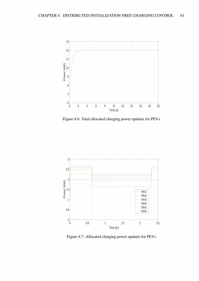
CHAPTER 4. DISTRIBUTED INITIALIZATION-FREE CHARGING CONTROL 61
0 2 4 6 8 10 12 14 16 18 20Time (s)
6
7
8
9
10
11
12
13
Pow
er
(kW
)
Figure 4.6: Total allocated charging power updates for PEVs
0 0.5 1 1.5 2 2.5Time (hr)
0
0.5
1
1.5
2
2.5
3
Pow
er
(kW
)
PEV1PEV2PEV3PEV4PEV5PEV6
Figure 4.7: Allocated charging power updates for PEVs

CHAPTER 4. DISTRIBUTED INITIALIZATION-FREE CHARGING CONTROL 62
0 0.5 1 1.5 2 2.5Time (hr)
-2
-1
0
1
2
3
4
5
6
Pow
er
(kW
)
Figure 4.8: Supply-demand mismatch updates for PEVs
0 0.5 1 1.5 2 2.5Time (hr)
0
0.2
0.4
0.6
0.8
1
Pow
er
(kW
)
PEV1PEV2PEV3PEV4PEV5PEV6
Figure 4.9: The SoC updates for PEVs

CHAPTER 4. DISTRIBUTED INITIALIZATION-FREE CHARGING CONTROL 63
Case 4.4.1. In this case, the total available charging power is assumed as 12kW. As shown
in Figs. 4.5 - 4.6, the charging rates of all PEVs quickly converge to their optimal values,
while the total allocated charging power converges to 12kW, i.e., the total available charging
power.
The plug-and-play adaptability of our strategy is investigated, e.g., 1) an EV arrives in the
charging station at an arbitrary time; 2) an EV leaves the charging station when its SoC is
charged to its desired value. The total available charging power is still 12kW. The communi-
cation network is weight-balanced, when PEVs are moving in and out. Here an imbalance-
correcting algorithm [116] is applied to this communication network design. Supposing that
each agent can correct its weight by sending and receiving information from its neighbours,
the digraph adapts and becomes weight-balanced in a finite time. Figs. 4.7 - 4.9 show the
charging power allocations of PEVs during their charging process, the demand-supply mis-
match and the SoC of PEVs. As shown in Fig. 4.7, the charging power allocations of each
PEV converge to their optimal values. When one PEV, e.g., PEV6, arrives at the charging
station, the charging power allocation can converge to the optimal values with the proposed
strategy. After PEV3 leaves the charging station, the proposed strategy guarantees that the
remaining PEVs can still reach their optimal charging rates by sharing the total available
charging power. As shown in Fig. 4.8,during the whole PEV charging process, the devia-
tions between the total available charging power and the total allocated charging power are
very small. Fig. 4.9 gives the SoC update of the PEV charging process when a PEV leaves or
arrives at the charging station. When PEV6 arrives at the charging station at a random time,
its SoC starts from 20% and increases during the charging process. The SoC of PEV3 drops
to zero because it has been charged to the desired SoC, and it is ready to depart from the
station. Therefore, the proposed strategy will have little effect on the frequency disturbance
of the system, which may be applied to isolated systems such as an autonomous microgrid.
Case 4.4.2. The effectiveness of the proposed strategy under a time-varying supply-demand
condition is validated in this case. An isolated microgrid consisting of DGs and loads is
considered here. Due to the intermittent nature of renewable energy sources, particularly
wind power generation, the generated power may fluctuate and cause a frequency fluctuation
problem in the microgrid. PEVs installed on the customer side are employed as a flexible

CHAPTER 4. DISTRIBUTED INITIALIZATION-FREE CHARGING CONTROL 64
0 0.5 1 1.5 2 2.5Time (hr)
0
0.5
1
1.5
2
2.5
3
Pow
er
(kW
)
PEV1PEV2PEV3PEV4PEV5PEV6
Figure 4.10: Allocated charging power updates for PEVs
0 0.5 1 1.5 2 2.5Time (hr)
-2
-1
0
1
2
3
4
5
6
Po
we
r (k
W)
Figure 4.11: Supply-demand mismatch updates for PEVs

CHAPTER 4. DISTRIBUTED INITIALIZATION-FREE CHARGING CONTROL 65
0 5 10 15 20 25 30 35 40 45 50
Time (s)
1
1.2
1.4
1.6
1.8
2
2.2
2.4
Po
we
r (
kW
)
Figure 4.12: Allocated charging power updates for 30-PEVs
load for alleviating frequency fluctuation [117]. To this end, we consider a time-varying non-
PEV load condition with the total available power given by Ptotal = 12000+700sin(0.005t).
The communication network and the other operating conditions are the same as those in
Case 4.4.1. As shown in Figs. 4.10 - 4.11, the allocated charging powers converge to
their op- timal values under the time-varying supply-demand condition, while the mismatch
between supply and demand power converges to zero. In addition, Fig. 4.11 shows that
the proposed strategy effectively offsets the supply-demand mismatch, which will help with
frequency fluctuation (caused by the intermittent nature of renewable sources) regulation.
Case 4.4.3. The scalability of the proposed strategy is validated. To do so, we implement the
optimal control strategy to both 30-PEV system and 60-PEV system, and The total available
charging power is supposed to be 60kW and 120kW, respectively. The communication
network is weight-balanced and strongly connected.
As shown in Fig. 4.12 and Fig. 4.14, the proposed strategy can guarantee the allocated
charging powers to converge to their optimal values within 25s. Figs. 4.13 - 4.15 illustrate
the deviations of demand and supply power can converge to zero. It is worth noting that
the convergence of the proposed algorithm is mainly determined by parameter selection and
the knowledge of the communication network. The convergence can be ensured for a large
number fleet by maintaining the inequality (4.25).

CHAPTER 4. DISTRIBUTED INITIALIZATION-FREE CHARGING CONTROL 66
0 5 10 15 20 25 30 35 40 45 50Time (s)
40
45
50
55
60
Pow
er
(kW
)
Figure 4.13: Supply-demand mismatch updates for 30-PEVs
0 5 10 15 20 25 30 35 40 45 50
Time (s)
1
1.2
1.4
1.6
1.8
2
2.2
2.4
Pow
er
(kW
)
Figure 4.14: Allocated charging power updates for 60-PEVs

CHAPTER 4. DISTRIBUTED INITIALIZATION-FREE CHARGING CONTROL 67
0 5 10 15 20 25 30 35 40 45 50Time (s)
80
85
90
95
100
105
110
115
120
Pow
er
(kW
)
Figure 4.15: Supply-demand mismatch updates for 60-PEVs
It should be noted that the proposed algorithm is applicable in a real scenario since the re-
quired communication network for data transmission is acceptable for a real communication
network and the computational cost is acceptable for running an embedded system.
4.5 Conclusion
In this chapter, a cooperative distributed control strategy is proposed for PEV optimal charg-
ing by maximizing the welfare and satisfaction of PEV customers while considering the
charging constraints of PEVs. The proposed distributed algorithm is implemented based on
MAS-framework under a directed communication graph, which is robust to dealing with
single-link failures compared with centralized methods. The initializing procedures are no
longer needed in this control design. Thus, the PEVs can start from any charging power
allocations. In addition, since the convergence of the proposed algorithm does not rely
on a specific graph, it allows plug-and- play operation during the PEV charging process.
Furthermore, the proposed distributed strategy can handle the time-varying supply-demand
mismatch problem in isolated systems.

Chapter 5
Distributed Agent Consensus-Based
Optimal Resource Management for
Microgrids
5.1 Introduction
This chapter considers the optimal resource management problem for an islanded microgrid.
Microgrids provide a promising approach to deal with challenges regarding the integration
of distributed renewable generation and ESSs. However, as indicated in Section 3.3.2, re-
source management in a microgrid encounters a new difficulty, i.e. supply-demand imbal-
ance, caused by the intermittence of renewable sources. Therefore, an optimal solution is
proposed to the resource management by enhancing communication and coordination un-
der a multi-agent system framework. An agent is a participant, for instance, the distributed
RGs/ESSs of the microgrid. With this MAS, the distributed optimal solution only utilizes
local information, and interacts with neighbouring agents. Thus, single-node congestion
is avoided since the requirement for a central control centre is eliminated, and it is robust
against single-link/node failures. The analysis will show that the proposed solution can
solve the resource management problem in an initialization-free manner. Additionally, the
68

CHAPTER 5. DISTRIBUTED OPTIMAL RESOURCE MANAGEMENT SYSTEMS 69
proposed strategy can maintain the supply-demand balance under a time-varying supply-
demand deviation.
5.2 Problem Formulation
The resource management of RGs is formulated to minimize the generation cost while sat-
isfying the supply-demand constraint and the RG constraints. In this section, the objective
function, while considering both RGs and parallel-connected ESSs costs, is constructed as:
Min C(PR, PE) = ∑i∈NRG
fi(PR,i(t))+ ∑j∈NESS
g j(PE, j(t)) (5.1)
where NRG and NESS are the sets of RGs and ESSs, respectively. fi(PR,i(t)) and g j(PE, j(t))
are the cost function for ith RG and jth ESS, for i ∈NRG and j ∈NESS. PR,i(t) and PE, j(t)
are the output power of ith RG and jth ESS. Moreover, define Ck(PR,i, PE, j) = fi(PR,i(t))+
g j(PE, j(t)) and C(PR, PE) = ∑k∈N Ck(PR,i, PE, j) with PR = [PR,i(t), . . . ,PR,n(t)]T ∈ Rn and
PE = [PE, j(t), . . . ,PR,n(t)]T ∈ Rn.
Then, the RG’s objective of economic dispatch is to minimize the curtailment of renewable
energy in a microgrid. To this end, the cost function of the ith RG is expressed as
fi(PR,i(t)) = aiPR,i(t)2 +biPR,i(t)+ ci (5.2)
where PmaxR,i is the predicted maximum power generation capacity of ith RG, and ai =
εi2Pmax
,
bi = −εi, and ci =εiPmax
2 , respectively. A trade-off factor εi difference between the ca-
pacity and generation cost, which can be selected according to the capacity required, the
installation and other costs known as ’balance of system cost’ for each type of renewable
source [70, 118]. The formulated objective function (5.2) has a similar format to the cost
function in [119, 120] with different the parameter setting. In addition, (5.2) indicates that
a lower power generation cost is realized when the deviation of actual output power PR,i(t)
between PmaxR,i is minimized. Hence, the minimization of renewable energy curtailment can
be derived by minimizing the generation cost of RGs [121].
Following [122],a convex quadratic cost function is adopted to represent the power loss of
ESSs during the charging/discharging process, i.e.,

CHAPTER 5. DISTRIBUTED OPTIMAL RESOURCE MANAGEMENT SYSTEMS 70
g j(PE, j(t)) = a jPE, j(t)2 +b jPE, j(t)+ c j (5.3)
where a j, b j and c j are the non-negative parameters of jth ESS, which can be selected in
terms of the Amoroso and Cappuccino’s experimental results [123].
5.2.1 Constraints
The physical limitations on the operation of the studied system are presented as follows:
Global Constraint
Since the change of frequency within a microgrid is mainly affected by the supply-demand
mismatch, the supply-demand balance should be maintained to ensure the stability of the
microgrid. To this end, the active power balance in a microgird can be expressed as:
PD(t) = ∑i∈NRG
PR,i(t)+ ∑j∈NESS
PE, j(t) (5.4)
where PD(t) is the total load demand.
Local Constraints
The actual output power of each RG and ESS should belong to a feasible range, i.e.,
PminR,i ≤ PR,i ≤ Pmax
R,i
PminE, j ≤ PE, j ≤ Pmax
E, j (5.5)
where PminR,i and Pmax
R,i are the lower and upper bound for the ith RG; PminE, j and Pmax
E, j are the
lower and upper bound for the jth ESS.

CHAPTER 5. DISTRIBUTED OPTIMAL RESOURCE MANAGEMENT SYSTEMS 71
5.2.2 Objective Function
Considering both the global constraints (5.4) and local constraints (5.5), the resource man-
agement problem is formulated as
Min C(PR, PE)
subject to
PD(t) = ∑i∈NRG
PR,i(t)+ ∑j∈NESS
PE, j(t),
PminR,i <PR,i < Pmax
R,i , for i ∈NRG
PminE, j <PE, j < Pmax
E, j , for j ∈NESS. (5.6)
Remark 5.2.1. In the formulation of the objective function, the cost function is used to re-
flect the operating cost of the islanded microgrid. The formulated cost function consists of
a generation cost of each RG and a charging/discharging cost of each BESS. The genera-
tion cost of RGs is formulated to minimize the curtailment of renewable energy when the
minimized generation cost is achieved. In the meantime, the cost function of BESSs rep- re-
sents the power losses during the charging/discharging process as indicated in [122], which
maximizes the actual power output of BESSs while minimizing the power losses. For this
reason, the total operating cost will be minimized by the proposed cost function.
The feasibility set and the solution set of the resource management problem is denoted by
FRM and F ∗RM, respectively. Denote PE = [PE,1, . . . ,PE,n]∈Rn and PR = [PR,1, . . . ,PR,n]∈Rn,
respectively. A useful Lemma in [113] is introduced as follows
Lemma 5.2.1. Since Ck(PR,i,CE, j) is convex, locally Lipschitz, and continuously differen-
tiable, the optimization problem has a solution (P∗R,P∗E)∈Rn if and only if ∃σ∈R such that σ1n ∈
∂PRC(PR,PE), and σ1n ∈ ∂PEC(PR,PE), and 1nP∗R +1nP∗E = PD.
5.3 Distributed solution of dynamic economic dispatch
The formulated problem (5.6) is a convex optimization problem with both equality and in-
equality constraints. Traditional centralized strategies may have some challenges, such as

CHAPTER 5. DISTRIBUTED OPTIMAL RESOURCE MANAGEMENT SYSTEMS 72
computation burden and non-timely response. In this section, in order to overcome these
challenges, we develop a distributed cooperative strategy to deal with the resource manage-
ment problem is developed, which only utilizes locally available information and interacts
with its adjacent agents.
5.3.1 Distributed Algorithm Design
Inspired by the dynamic average consensus estimation method proposed in [124], a dis-
tributed solution is developed for resource management, which allows the power allocation
of RGs and ESSs to start from any initial condition. The distributed algorithm is formulated
as:
PR,i =− ∑h∈NRG
aih(∂PR,iCi(PR,i,PE, j)
−∂PR,hCh(PR,h,PE, j)), (5.7a)
PE, j =− ∑k∈NESS
a jk(∂PE, jCi(PR,i,PE, j)
−∂PE,kCk(PR,i,PE,k))+ γx j, (5.7b)
x j =−β(x j− (bi0PD−PE, j−PR,i))
−α ∑k∈NESS
a jk(x j− xk)− ∑k∈NESS
a jk(η j−ηk), (5.7c)
η j =αβx j, (5.7d)
where α, β, γ∈R>0 are the parameters to be designed. NRG and NESS denotes the neighbour
set of ith RG and jth ESS, respectively. In addition, x j is designed to track the difference
between supply and demand, PD−1Tn PE−1T
n PR. Both RGs and ESSs are deployed through
a Laplacian-gradient algorithm to explore the minimization of the generation cost. Mean-
while, we introduce a feedback element, γx j for jth ESS to meet the supply-demand equality
condition.
Remark 5.3.1. Note that the renewable generation may not be considered as dispatchable if
it is controlled in maximum peak power tracking (MPPT) mode because of their intermittent
and irregular nature. because of its intermittent and irregular nature. As a result, RGs
are not used to compensate the supply-demand mismatch. Thus, only ESSs are deployed

CHAPTER 5. DISTRIBUTED OPTIMAL RESOURCE MANAGEMENT SYSTEMS 73
to maintain the supply-demand balance in the control design. The feedback term is only
introduced for the jth ESS to satisfy the supply-demand equality condition. Furthermore,
the ith RG only implements (5.7b) to explore the minimization of its own generation cost.
5.3.2 Convergence Analysis
The algorithm is rewritten in a compact form for convergence analysis as
PE =−LE∂PEC(PR,PE)+ γx, (5.8a)
PR =−LR∂PRC(PR,PE), (5.8b)
x =−αLEx−β(x− (B0PD−PE −PR))−LEη, (5.8c)
η = αβx, (5.8d)
where x, η are the column vectors containing xi, and ηi, respectively. LE and LR denote the
corresponding Laplacian matrix of network connections of ESSs and RGs, respectively.
Let Pk = PR,i +PE, j, and P = [P1, . . . ,Pn] ∈ Rn. The ω-limit set of the trajectories of (5.7)
under any initial condition in Rn×Rn×Rn is first characterized. Then, with T=Rn×Rn×
Rn and T0 = HPD×H0×H0, the following lemma is introduced.
Lemma 5.3.1. The ω-limit set of any trajectory of (5.8) with any initial condition in (Pk,0,x0,η0)∈
T is contained in T0.
Proof. Defining φ(t) = 1Tn P−PD, one has
φ(t) = 1Tn γx(t), (5.9)
and
φ(t) = 1Tn γx(t)
=−1Tn βγx(t)+1T
n βγ(x− (B0PD−P))
=−βγφ(t)−βφ(t). (5.10)
The system can be rewritten as a linear system z = Az with z = [z1,z2]T , and z1 = φ(t),z2 =

CHAPTER 5. DISTRIBUTED OPTIMAL RESOURCE MANAGEMENT SYSTEMS 74
φ(t). The system matrix is
A =
0 1
−βγ −β
.Let R ∈ R2×2 be
R =1
2γβ2
β2 +βγ+(βγ)2 β
β 1+βγ
, (5.11)
which satisfies AT R+RA+ I = 0. Define Vz = zT Rz as a Lyapunov function candidate, and
the derivative of Vz is
Vz =−zT z. (5.12)
Therefore, it can be deduced that (φ(t); φ)→ 0. Furthermore, φ = 0 implies that 1Tn PE(t)+
1Tn PR(t)→ PD and 1T
n x(t)→ 0. Note that 1Tn η = 0, as 1T
n x(t)→ 0.
Remark 5.3.2. The proof of Lemma 5.3.1 establishes the exponential stability of the de-
mand mismatch dynamics. With the Theorem 5.4 in [125], it can ensure the input-to-state
stability(ISS). Thus it is robust to arbitrary bounded perturbations. Additionally, from the
Lyapunov equation Vz = zT Rz, it follows Theorem 4.6 in [125] that gives the convergence
rate as ∥∥x(t)∥∥≤√λmax(R)
λmin(R)e
−1λmax(R)
∥∥x(0)∥∥ . (5.13)
The demand mismatch dynamics depends on the topology of the communication network.
However, the convergence rate does not directly depend on the knowledge of the Laplacian
matrix.
We are now ready to complete the convergence analysis. By applying (5.8), the trajectories
of the actual output power of RGs and their parallel-connected ESSs converge to the solution
of the optimization problem.
Theorem 5.3.1. The trajectories of (5.8) converge to the solution of the optimal charging
problem if α,β,γ ∈ R>0 satisfy the following conditions, i.e.,
βλmax(LTR LR)
2λ2(LR +LTR )≥ 0, (5.14)

CHAPTER 5. DISTRIBUTED OPTIMAL RESOURCE MANAGEMENT SYSTEMS 75
andγ
αβλ2(LE +LTE )
+βλmax(LT
E LE)
2< λ2(LE +LT
E ). (5.15)
Proof. A change of coordinates is performed to shift the equilibrium point of (5.8) to the
origin, i.e., η = LE −β(B0PD−PE −PR). Then, the dynamics (5.8) can be transformed as
PE =−LEξ1 + γx,
PR =−LRξ2,
x =−αLEx−β(x− (B0PD−PE −PR))−LEη,
˙η = αβLEx+ γβx−βLEξ1−βLRξ2, (5.16)
with ξ1 ∈ ∂PEC(PR,PE) and ξ2 ∈ ∂PRC(PR,PE).
Next step is to prove that the trajectories of (5.8) converge to the optimal solution of the
formulated problem in the new coordinates.
Consider a candidate Lyapunov function
V =C(PR,PE)+12
γβ‖θ1‖2 +12‖θ2‖2 . (5.17)
where an additional transformation is introduced to more easily identify the candidate Lya-
punov function, with θ1 = x and θ2 = βx+ η.
Then the time derivative of (5.17) along the trajectories of (5.8) is given as
V =−ξT1 LEξ1 + γξ
T1 θ1−ξ
T2 LRξ2− γαβθ
T1 LEθ1
−βθT2 θ2−βθ
T2 LEξ1−βθ
T2 LRξ2
=−12
ξT1 (LE +LT
E )ξ1 + γξT1 θ1−
12
ξT2 (LR +LT
R )ξ2
− 12
γαβθT1 (LE +LT
E )θ1−β‖θ2‖2−βθT2 LEξ1−βθ
T2 LRξ2 (5.18)
Since the directed graph G is strongly connected and weight-balanced with the fact that

CHAPTER 5. DISTRIBUTED OPTIMAL RESOURCE MANAGEMENT SYSTEMS 76
1Tn θ1 = 0 for (PE ,PR,θ1,θ2) ∈ T0, one has
V ≤−12
λ2(LE +LTE )
∥∥∥∥ξ1−1n
1Tn 1nξ1
∥∥∥∥2
+ γ(ξ1−1n
1Tn 1nξ1)
Tθ1
− 12
λ2(LR +LTR )
∥∥∥∥ξ2−1n
1Tn 1nξ2
∥∥∥∥2
−β‖θ2‖2
− 12
γαβλ2(LE +LTE )‖θ1‖2−βθ
T2 LE(ξ1−
1n
1Tn 1nξ1)
−βθT2 LR(ξ2−
1n
1Tn 1nξ2) (5.19)
Defining ψ1 = ξ1− 1n(1
Tn 1nξ1), ψ2 = ξ2− 1
n(1Tn 1nξ2) and υT
1 = [ψT1 ,θ
T1 ,θ
T2 ], υT
2 = [ψT2 ,θ
T2 ],
we have
V ≤ υT1 J1υ1−υ
T2 J2υ2, (5.20)
where
J1 =
−12λ2(LE +LT
E )In MT12
M12 M22
,
with MT12 =
[12γIn −1
2βLTE
]. and furthermore, M22 =
−12αβγλ2(LE +LT
E )In 0
0 −βIn
and
J2 =
−12λ2(LR +LT
R )In −12βLT
R
−12βLR 0
.Resorting to the Schur complement, J1 is negative definite if
−12
λ2(LE +LTE )In +
γ
2αβλ2(LE +LTE )
In +β
4LT
E LE
is negative definite, and J2 is positive definite if
βλmax(LTR LR)
2λ2(LR +LTR )
(5.21)
is positive definite, respectively. Furthermore, we can conclude that V ≤ 0 by applying
(5.15) and (5.14). Hence, with the application of LaSalle Invariance principle, we deduce
that V = 0 iff ψ1 = ψ2 = θ1 = θ2 = 0 , which implies that ∂PEC(PR,PE) ∈ span1n and
∂PRC(PR,PE)∈ span1n. Recalling the Lemma 5.3.1 and the characterization of optimizers
in Lemma 5.2.1, it indicates (P∗E ,P∗R) is a solution of the optimization problem.

CHAPTER 5. DISTRIBUTED OPTIMAL RESOURCE MANAGEMENT SYSTEMS 77
Figure 5.1: General operation diagram of an agent.
Remark 5.3.3. The local inequality constraints are taken into account by applying addi-
tional projection operations to each RG and ESSs. As shown in the literature [126, 127],
the projection operation does not affect the convergence analysis of the distributed optimal
strategy.
Remark 5.3.4. It might be possible to include the operating limits of the power network,
such as voltage and line flow limits in the proposed algorithm by applying the projec-
tion method, which may lead to different optimization results. Additionally, the proposed
method can also deal with the model of the transmission loss in [128], which assumes each
agent could estimate the power loss of the line adjacent to it. With the available estimation
value, each agent could add this value to the load quantity, which would result in the network
discovering a new optimization result that considers power loss.
5.4 Simulation Results and Analysis
In the following case studies, the designed parameters are chosen as α = 14, β = 0.6, γ = 3,
which satisfies the condition specified in Theorem 5.3.1. The parameters of RGs and ESSs
are summarized in Table 5.1. Each participant in the microgrid is regarded as an agent that
equips with two level controls, i.e. top level control and bottom level control as shown in
Fig. 5.3.2.

CHAPTER 5. DISTRIBUTED OPTIMAL RESOURCE MANAGEMENT SYSTEMS 78
Figure 5.2: IEEE 14-bus system.
The first two cases test the proposed control strategy based on the IEEE 14-bus system with
the base power Pbase=100kW, and the communication topology is shown as Fig. 5.2. In
Case 5.1, the optimal resource management problem is studied under both constant supply-
demand deviation and time-varying deviation conditions. Case 5.2 investigates the perfor-
mance of the proposed strategy under the link/node failures. To accomplish the tractability
of the demonstration, it is assumed that if the single-link/node failure occurs in the commu-
nication topology, the rest of the weighted-balanced digraph should still remain connected,
and thus the remaining nodes would be able to operate with their neighbouring nodes con-
tinuously [47]. Finally, the scalability analysis is validated in Case 5.3 in the IEEE 162-bus
system with various RGs and ESSs, such as WTs, PVs, Solar thermal, BESSs and fuel
cells. Without loss of generality, it is assumed that ESS1 knows the total supply-demand
mismatch.

CHAPTER 5. DISTRIBUTED OPTIMAL RESOURCE MANAGEMENT SYSTEMS 79
Table 5.1: Simulation Parametersa j b j Pmin
E, j (p.u.) PmaxE, j (p.u.)
ESSs
ESS1 0.83 0.007 0 50ESS2 0.79 0.006 0 50ESS3 0.90 0.009 0 50ESS4 0.93 0.012 0 50ESS5 0.78 0.008 0 50
PredicatedMaximumCapacity
PminR,i (p.u.) Pmax
R,i (p.u.) εi
PVsPV1 60 0 60 0.1PV2 62 0 65 0.2PV3 65 0 65 0.1
WTsWT1 67 0 67 0.1WT2 68 0 68 0.2
5.4.1 Case 5.1
In this case, the performance of the proposed distributed strategy for resource management
is investigated in the IEEE 14-bus system. The designed communication network of agents
can be independent of the physical bus connections, which is a directed network in this
simulation study.
1) Constant Supply-demand Mismatch Condition: The total supply-demand mismatch
is assumed as 500 p.u.. As shown in Figs. 5.3 and 5.4, the power allocations of
RGs and parallel-connected ESSs quickly converge to their optimal values, while the
supply-demand balance converges to zero, i.e., the optimization objective is achieved.
2) Time-varying Supply-demand Mismatch Condition: if renewable energy resources
are controlled by MPPT algorithms, this may cause a time-varying supply-demand
imbalance when the available renewable generation cannot meet load demands. As
a result, in this subcase, the time-varying imbalance is modelled by a time-varying
function, i.e., PD = 500+10sin(0.05t) p.u.. The simulation results are shown in Figs.
5.5 and 5.6. The allocated actual powers converge to their optimal values, and the
deviation between supply and demand power is close to zero.

CHAPTER 5. DISTRIBUTED OPTIMAL RESOURCE MANAGEMENT SYSTEMS 80
0 5 10 15
Time (s)
0
10
20
30
40
50
60
70
Po
we
r (p
.u.)
ESS1 ESS2 ESS3 ESS4 ESS5 PV1 PV2 PV3 WT1 WT2
Figure 5.3: The actual output power of RGs and ESSs
In this case study, it is shown that the proposed strategy effectively offsets the supply-
demand mismatch, which will help with frequency regulation in an islanded microgrid.
5.4.2 Case 5.2
The robustness of single link/node failure is investigated in this case. In the first subcase,
it is assumed that a breakdown of the transmission line for ESS3 is at 10s, and it can still
communicate with its neighbours. Because RGs are not used for tackling demand mismatch,
the remaining ESSs have to undertake the supply-demand balance in a fast response time.
At 30s, the emergency line is employed, and hence ESS3 is plugged in to support the load
demand. The results are shown in Figs. 5.7 - 5.9. After ESS3 is unplugged, the power
allocations of all participants converge to the new optimal values. Furthermore, the supply-
demand mismatch can be handled by the remaining ESSs. When ESS3 is connected again,
all the results converge to those of the previous ones.
Next, the second subcase is considered when ESS3 fails to operate at 6s and recovers at
40s. Upon failure, ESS3 loses communication with its neighbours, and the remaining ESSs
remain connected to support the load demand. The results in Fig. 5.10 and Fig. 5.11
show that the other participants can converge to a new optimal operation condition, and the
supply-demand mismatch is eliminated when ESS3 fails. Moreover, the results converge to

CHAPTER 5. DISTRIBUTED OPTIMAL RESOURCE MANAGEMENT SYSTEMS 81
0 5 10 15
Time (s)
-10
0
10
20
30
40
50
60
70
80
90
Po
we
r (p
.u.)
Pd
Figure 5.4: The supply-demand mismatch update
0 5 10 15
Time (s)
10
20
30
40
50
60
70
Po
we
r (p
.u.)
ESS1 ESS2 ESS3 ESS4 ESS5 PV1 PV2 PV3 WT1 WT2
Figure 5.5: The actual output power of RGs and ESSs

CHAPTER 5. DISTRIBUTED OPTIMAL RESOURCE MANAGEMENT SYSTEMS 82
0 5 10 15 20 25 30 35 40
Time (s)
-10
0
10
20
30
40
50
60
70
80
Po
we
r (p
.u.)
Pd
Figure 5.6: The supply-demand mismatch update
0 5 10 15 20 25 30 35 40
Time (s)
0
10
20
30
40
50
60
70
Po
we
r (p
.u.)
ESS1 ESS2 ESS3 ESS4 ESS5 PV1 PV2 PV3 WT1 WT2
Figure 5.7: The actual output power of RGs and ESSs during the single link failure

CHAPTER 5. DISTRIBUTED OPTIMAL RESOURCE MANAGEMENT SYSTEMS 83
0 5 10 15 20 25 30 35 40
Time (s)
420
440
460
480
500
520
540
Pow
er
(p.u
.)
Figure 5.8: The supply-demand mismatch update
0 5 10 15 20 25 30 35 40
Time (s)
-40
-20
0
20
40
60
80
Pow
er
(p.u
.)
Pd
Figure 5.9: Total allocated output power

CHAPTER 5. DISTRIBUTED OPTIMAL RESOURCE MANAGEMENT SYSTEMS 84
0 10 20 30 40 50 60
Time (s)
0
10
20
30
40
50
60
70
Pow
er (
p.u
.)
ESS1 ESS2 ESS3 ESS4 ESS5 PV1 PV2 PV3 WT1 WT2
Figure 5.10: The actual output power of RGs and ESSs during the single node failure
those of the previous ones after ESS3 is repaired.
It should be noted that during single link/node failure, the supply-demand deviations are
small. Therefore, the proposed strategy will have little effect on the frequency disturbance
of the system, which may be applied to isolated systems such as an autonomous microgrid.
Remark 5.4.1. One of the necessary conditions for the convergence of the proposed algo-
rithm is the connectivity of the communication network. Therefore, when single- link/node
failure occurs, the optimal solution is guaranteed if the communication network remains
connected. Distributed information is also used in the proposed algorithm rather than global
information, which is robust to dealing with link failures if the failure does not affect the
connectivity of the communication network. Also, when one node fails to communicate
with the other neighbours, the remaining groups of nodes can continue their operations if
the network is connected.
5.4.3 Case 5.3
The scalability of the proposed strategy is validated. This is achieved by implementing the
optimal control strategy to the modified IEEE 162-bus system. There are three types of RGs
in this system, i.e., eight PVs, eight WTs and one solar thermal, and two types of ESSs, i.e.,

CHAPTER 5. DISTRIBUTED OPTIMAL RESOURCE MANAGEMENT SYSTEMS 85
0 10 20 30 40 50 60
Time (s)
-40
-20
0
20
40
60
80
100
120
Pow
er (
p.u
.)
Figure 5.11: The supply-demand mismatch update
battery storage system and fuel cells. The cost functions of the fuel cell and solar thermal
are based on the cost model in [129, 130], respectively. The communication network is
weight-balanced and strongly connected. The initial condition is given by [131] with a total
load demand of 18422 MW.
As shown in Fig. 5.12 and Fig. 5.13, the proposed strategy can guarantee the allocated
charging powers to converge to their optimal values within 12s while the deviations of de-
mand and supply power converge to zero, demonstrating that the proposed algorithm is
scalable.
5.5 Conclusion
In this chapter, a MAS-based distributed optimal strategy has been proposed to the optimal
resource management in an islanded microgrid. The proposed strategy not only minimizes
the generation cost to all participants, but also maintains the supply-demand equality condi-
tion within the microgrid system. The effectiveness of the proposed distributed strategy is
demonstrated by the simulation that uses the IEEE test systems. To tackle the more practical
constraints of resource management, voltage limits, line capacities, and network reconfigu-
ration will be considered in future work.

CHAPTER 5. DISTRIBUTED OPTIMAL RESOURCE MANAGEMENT SYSTEMS 86
0 2 4 6 8 10 12 14 16 18 20
Time(s)
-500
0
500
1000
1500
2000
Po
we
r (
MW
)
Figure 5.12: The actual power output of RGs and ESSs
0 2 4 6 8 10 12 14 16 18 20
Time (s)
0
200
400
600
800
1000
1200
1400
Pow
er (
MW
)
Figure 5.13: The supply-demand mismatch update

Chapter 6
Distributed Finite-Time Optimal
Resource Management for Microgrids
Based on Multi-Agent Framework
6.1 Introduction
The key issues proposed in Section 3.3.2 mean that a fast convergence algorithm is required
to coordinate both dispatchable and non-dispatchable energy resources to effectively main-
tain microgrid stability under different operation modes.
In this chapter, a two-level optimization system is proposed for optimal resource manage-
ment with a fast convergence speed. At the top level, the proposed algorithm generates a
reference point of optimal power output through local communication. The algorithm only
requires information among neighbouring participants without a central control coordina-
tion, and simultaneously accomplishes resource optimization in a finite-time while respect-
ing system constraints. The bottom-level control is responsible for the reference tracking
of each corresponding participant in a microgrid. The convergent rate of the proposed al-
gorithm is compared with other consensus-based algorithms through simulation studies.
Furthermore, an actual islanded system is presented to demonstrate the overall effectiveness
of the proposed strategy.
87

CHAPTER 6. FINITE-TIME DISTRIBUTED RESOURCE MANAGEMENT 88
6.2 Multi-agent System Architecture of a Microgrid
In this section, the topology of the communication network for a microgrid is first intro-
duced. Next, agents are defined in a microgrid context, and the cost function of each type of
agents is formulated for distributed optimization.
6.2.1 Multi-agent System Framework
In the MAS framework, a microgrid consists of a utility grid, non-dispatchable DGs includ-
ing WTs and PVs, conventional dispatchable synchronous generators (SGs), ESSs and non-
controllable load demands. A Point of Common Coupling (PCC) of the utility grid is used to
measure the power delivered/withdrawn and decide the operation mode of the micro- grid.
In the MAS framework, each participant in the microgrid is assigned to an intelligent agent
that is able to interconnect with its adjacent agents to accomplish established objec- tives. A
two-level control model, namely the top-level control and bottom-level control, is deployed
to each agent as depicted in Fig. 6.1. The top-level control is a communication network for
each agent to transfer information that is generated by an optimal strategy. Both the control
mode and the physical agent platform are located at the bottom-level control. According to
the control schemes in [73],the control mode is used to adjust the power output of the agent
to the reference signal generated by the top-level, and the settings of different control modes
can be decided by the agents local operation conditions. Furthermore, the physical agent
platform is the electrical components that transmit the power generated/consumed.
6.2.2 The Agent Description under MAS Framework
In this section, agents are defined in the microgrid context under the proposed MAS frame-
work, and the corresponding cost functions are defined for the algorithm design.

CHAPTER 6. FINITE-TIME DISTRIBUTED RESOURCE MANAGEMENT 89
Figure 6.1: The communication network of agents in a microgrid
Dispatchable Agents
Conventional Generator Agents Conventional generator agents include fuel generators
and gas plants. The generation cost of this type of agent is usually expressed as a typical
quadratic function of active power output, i.e.,
Ck(PG,k) =12
akP2G,k +bkPG,k + ck, Pmin
G,k ≤ PG,k ≤ PmaxG,k (6.1)
where non-negative ak, bk, and ck are the cost coefficients for kth generator; PminG,k and Pmax
G,k
are the lower and upper bounds of the power output, respectively. The marginal cost function
is the derivative of the cost function with respect to PG,k, which is used to later algorithm
design.
Storage Agents Agents The storage agents can be treated as a dispatchable agent since
they have the capacity to transfer power to absorb excessive power and compensate for
insufficient power bidirectionally. Integrating storage agents to a microgrid may require
additional costs, and thus, it is ideal to charge the storage agents when the marginal cost
is low, and discharge them when the electricity rate is high otherwise [132]. Furthermore,
battery life directly depends on different DoD scenarios in each cycle time [133], and the
degradation cost is also an essential factor that may affect the economic decision for batteries
[134]. To this end, inspired by [132], a general cost function for the jth battery is proposed

CHAPTER 6. FINITE-TIME DISTRIBUTED RESOURCE MANAGEMENT 90
by considering DoD:
C j(PB, j) =12
a j(PB, j +3PmaxB, j (DoD))2
+b j((PB, j +3PmaxB, j (DoD))+ c j, Pmin
B, j ≤ PB, j ≤ PmaxB, j (6.2)
where a j, b j, and c j are the non-negative quadratic coefficients; PminB, j and Pmax
B, j are the
minimal and maximum charging rate, respectively. The DoD is the current depth of charge,
and the marginal cost is defined as the derivative of the cost function with respect to PB, j.
From the cost function design, it is worth noting that the marginal cost is proportional to the
DoD and the power withdrawn.
Utility Agent When the microgrid is operated under the grid-connected mode, the utility
agent will monitor the power transfer between the utility grid and the microgrid through the
PCC. Accordingly, the microgrid updates its current electricity rate based on the broadcast-
ing of the utility grid. The cost function can be assumed as a function with constant marginal
cost [132],
CU = Pr×PU (6.3)
where Pr is the current electricity rate and PU is the exchanged power between the utility
and the microgrid. During the grid-connected mode operation, the marginal cost of each
dispatchable agent should be equal to the marginal cost given by the utility grid, which is
equal to the electric rate.
Nondispatchable Agents
Renewable Agents The RGs, including WTs and PVs, are considered as non-dispatchable
since they are usually controlled in MPPT mode. Therefore, the forecast of their generation
cannot be accurate because of the stochastic property and intermittency.
Load Demand Agents The load demands, consisting of industrial and residential loads,
have the stochastic property of the consumer behaviours, so they cannot be treated as dis-
patchable due to the unpredictable nature of power requirements.

CHAPTER 6. FINITE-TIME DISTRIBUTED RESOURCE MANAGEMENT 91
Due to the intermittency of renewable generation, the operating condition of a microgrid
may change frequently and unexpectedly. In order to ensure the performance and stability
of the microgrid, the system should converge to the required target in a timely manner. As
a result, a faster convergence rate of a distributed optimal solution is required to meet the
challenges of microgrid development.
6.3 Finite-time Distributed Optimal Solution for the Islanded
Microgrid
In this section, a finite-time distributed optimal solution is developed for the islanded mi-
crogrid to address the problems in the centralized strategies in the microgrid application.
The islanded microgrid should ensure supply-demand balance in a cost-effective way. To
this end, the objective for agents in an islanded microgrid is to balance supply and demand,
and minimize generation/operation costs in the meantime. The objective function can be
formulated as:
Min ∑k⊆G
Ck(PG,k)+ ∑j⊆B
C j(PB, j)
s.t PD = PL−PR = ∑k⊆G
PG,k + ∑j⊆B
PB, j
PminG,k ≤ PG,k ≤ Pmax
G,k
PminB, j ≤ PB, j ≤ Pmax
B, j (6.4)
where PD is the net power demand; PL and PR are all demands of load agents and all non-
dispatchable generation, respectively.
For convenience, we denote Pi as the output power, and Pmini and Pmax
i as the lower and
upper bound of ith dispatchable agent, respectively. We further define ωi, σi and ci as the
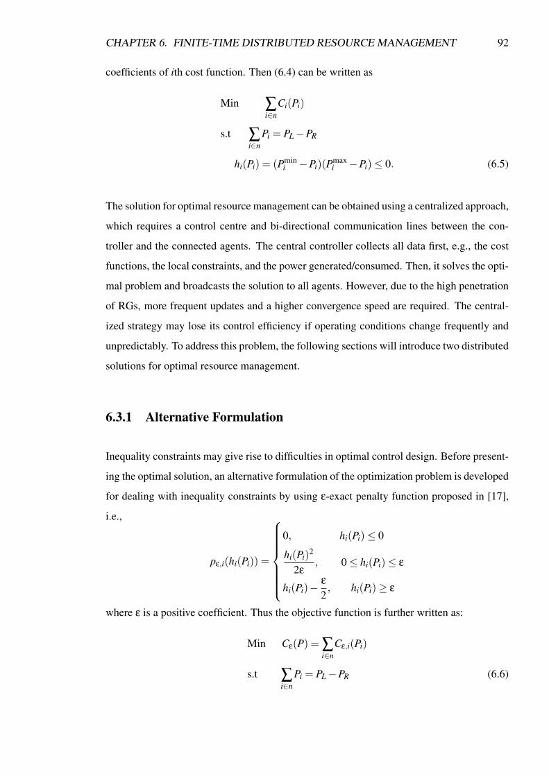
CHAPTER 6. FINITE-TIME DISTRIBUTED RESOURCE MANAGEMENT 92
coefficients of ith cost function. Then (6.4) can be written as
Min ∑i∈n
Ci(Pi)
s.t ∑i∈n
Pi = PL−PR
hi(Pi) = (Pmini −Pi)(Pmax
i −Pi)≤ 0. (6.5)
The solution for optimal resource management can be obtained using a centralized approach,
which requires a control centre and bi-directional communication lines between the con-
troller and the connected agents. The central controller collects all data first, e.g., the cost
functions, the local constraints, and the power generated/consumed. Then, it solves the opti-
mal problem and broadcasts the solution to all agents. However, due to the high penetration
of RGs, more frequent updates and a higher convergence speed are required. The central-
ized strategy may lose its control efficiency if operating conditions change frequently and
unpredictably. To address this problem, the following sections will introduce two distributed
solutions for optimal resource management.
6.3.1 Alternative Formulation
Inequality constraints may give rise to difficulties in optimal control design. Before present-
ing the optimal solution, an alternative formulation of the optimization problem is developed
for dealing with inequality constraints by using ε-exact penalty function proposed in [17],
i.e.,
pε,i(hi(Pi)) =
0, hi(Pi)≤ 0
hi(Pi)2
2ε, 0≤ hi(Pi)≤ ε
hi(Pi)−ε
2, hi(Pi)≥ ε
where ε is a positive coefficient. Thus the objective function is further written as:
Min Cε(P) = ∑i∈n
Cε,i(Pi)
s.t ∑i∈n
Pi = PL−PR (6.6)

CHAPTER 6. FINITE-TIME DISTRIBUTED RESOURCE MANAGEMENT 93
where Cε,i(Pi) = Ci(Pi)+ µpε,i(hi(Pi)), and P = [P1, . . . ,Pn]T . µ is a positive weight of the
penalty function.
Let P∗ = [P∗1 , . . . ,P∗n ]
T be the optimal solution for (6.5), and P∗ = [P∗1 , . . . , P∗n ]
T be the so-
lution for (6.6). Then, following Proposition 6 in [17], for µ = 1−n1−√
nµ∗, the relationship
between (6.5) and (6.6) is
0≤C(P∗)−Cε(P∗)≤ εµn, (6.7)
where µ∗ > maxη∗ with η∗ = η∗1, . . . ,η∗n is the Lagrange multiplier vector satisfying
the KarushKuhnTucker (KKT) condition [135]. According to the Proposition 4 in [136], the
upper bound of η∗ is given as
maxη∗i ni=1 ≤
2maxmaxPi∈Pfea,i
∣∣OCi(Pi)∣∣n
i=1
minPMi −Pm
i ni=1
, (6.8)
where OCi(Pi) is the gradient of Ci(Pi), and Pfea,i = Pi ∈ R |∑i∈n Pi = PL−PR and (Pmini −
Pi)(Pmaxi −Pi)≤ 0, for i ∈ n.
Remark 6.3.1. To ensure the ε-solution is equal to the solution of the original optimization
problem exactly, the local bound of each dispatchable agent is further modified as hi(Pi) =
(Pmini −Pi)(Pmax
i −Pi)+ ε ≤ 0 that can meet the accurate requirement of the system. Note
that s can be chosen to be significantly small so that it does not affect the convergence of
the original problem. After the change of local bounds, the ε-feasible set is the same as the
feasible set of the original optimization problem. The proof can be obtained by adopting a
similar approach in [17].
6.3.2 Finite-time Distributed Optimal Energy Management
By invoking the ε-penalty function, a finite-time distributed optimal solution is proposed to
solve the optimization problem (6.6). The update dynamics for ith dispatchable agent is
Pi =∑j∈n
ai j(OCε, j(Pj)−OCε,i(Pi))2− p
q
+ ∑j∈n
ai j(OCε, j(Pj)−OCε,i(Pi))pq (6.9)
where p and q are the positive odd integers satisfying p < q. The dynamics is distributed
in the sense that each dispatchable agent only requires local available information and the
information from its adjacent agents through a local communication network.

CHAPTER 6. FINITE-TIME DISTRIBUTED RESOURCE MANAGEMENT 94
Theorem 6.3.1. Consider the optimization problem in (6.6) with the dynamics (9), the fea-
sible set Pfea is time-invariant, and any trajectory starting from Pfea converges to the solution
set of (6.6) in a finite-time.
Proof. A candidate function V1 = |∑ni=1 Pi| is considered since the active power of ESSs
would be negative/positive when they are charged/discharged. Also it should be noted that
PD 6= 0, we only consider the cases for PD > 0 or PD < 0 accordingly. Firstly, if ∑ni=1 Pi > 0,
V1 = ∑ni=1 Pi and the derivative of V1 is
V1 =n
∑i=1
∑j∈n
ai j(OCε, j(Pj)−OCε,i(Pi))2− p
q
+n
∑i=1
∑j∈n
ai j(OCε, j(Pj)−OCε,i(Pi))pq = 0. (6.10)
Then, if ∑ni=1 Pi < 0, V1 =−∑
ni=1 Pi and the derivative is
V1 =−
n
∑i=1
∑j∈n
ai j(OCε, j(Pj)−OCε,i(Pi))2− p
q
+n
∑i=1
∑j∈n
ai j(OCε, j(Pj)−OCε,i(Pi))pq
= 0. (6.11)
From the above results, it concludes that the total power output of network is conserved and
the feasible set Pfea is time-invariant.
Next, we show that the trajectories starting from Pfea will converge to the solution set in a
finite-time manner. Note that the solution to (6.6) is unique so that P∗ will be the unique
solution to the minimization problem. Denote V2 = ∑ni=1Cε,i(Pi)−∑
ni=1Cε,i(P∗i ) as a candi-
date function. It is worth noting that V2 ≥ 0, and V2 = 0 when Pi = P∗. From (6.9), and let
ξi ∈ OCε,i(Pi),

CHAPTER 6. FINITE-TIME DISTRIBUTED RESOURCE MANAGEMENT 95
V2 =n
∑i=1
ξi[∑j∈n
ai j(ξ j−ξi)2− p
q + ∑j∈n
ai j(ξ j−ξi)pq ]
=12
n
∑i, j=1
ai j(ξi−ξ j)(ξ j−ξi)2− p
q +12
n
∑i, j=1
ai j(ξi−ξ j)(ξ j−ξi)pq
=− 12
n
∑i, j=1
ai j(ξ j−ξi)3q−p
q − 12
n
∑i, j=1
ai j(ξ j−ξi)q+p
q
=− 12
n
∑i, j=1
[a2q
3q−pi j (ξ j−ξi)
2]3q−p
2q − 12
n
∑i, j=1
[a2q
q+pi j (ξ j−ξi)
2]q+p2q . (6.12)
Following the Corollary 2 in [137] and Lemma 3.4 in [138], it can be obtained that
V2 ≤−12
np−q
qn
∑i, j=1
[a2q
3q−pi j (ξ j−ξi)
2]3q−p
2q − 12
n
∑i, j=1
a2q
q+pi j (ξ j−ξi)
2
q+p2q
=−12
np−q
q [2ξT LBξ]
3q−p2q − 1
2[2ξ
T LCξ]q+p2q (6.13)
where ξ = [ξ1, . . . ,ξn]T . Consider the graphs GB and GC with the adjacency matrices AB =
[aBi j]n×n and AC = [aC
i j]n×n, respectively. Then LB and LC are the corresponding Laplacian
matrices of GB and GC respectively. Define
ΓB = 2ξT LBξ≥ 2λ2(LB)
∥∥∥∥ξ− 1n(1T
n ξ)1Tn
∥∥∥∥2
2(6.14)
ΓC = 2ξT LCξ≥ 2λ2(LC)
∥∥∥∥ξ− 1n(1T
n ξ)1Tn
∥∥∥∥2
2. (6.15)
Since Cε(P) is strongly convex, for P = [P1, . . . , Pn], it follows that
Cε(P)≥Cε(P)+(ξ− 1n(1T
n ξ)1Tn )(P−P)+
k2
∥∥∥P−P∥∥∥2
. (6.16)
It is worth noting that the minimum of (6.16) is Cε(P)− 12k
∥∥∥ξ− 1n(1
Tn ξ)1T
n
∥∥∥ for constant P.
For P = P∗, we have V2 ≤− 12k
∥∥∥ξ− 1n(1
Tn ξ)1T
n
∥∥∥. Therefore,
V2 ≤−12
np−q
q [4kλ2(LB)V2]3q−p
2q − 12[4kλ2(LC)V2]
q+p2q
≤−12
np−q
q [4kλV2]3q−p
2q − 12[4kλV2]
q+p2q
=−12
[n
p−qq [4kλV2]
q−pq +1
]([4kλV2]
q+p2q ), (6.17)
where λ = min λ2(LB), λ2(LC)> 0. Let δ =√
4kλV2, then
δ =−np−q
q λδ2q−p
q −λδpq . (6.18)

CHAPTER 6. FINITE-TIME DISTRIBUTED RESOURCE MANAGEMENT 96
With Lemma 4.1 in [138] and Comparison Lemma in [125], we conclude that
limt→T1
V2 = 0, (6.19)
where T1 is given by
T1 ≤πqn
q−p2q
2λ(q− p). (6.20)
Note that V2 → 0 implies ∑ni=1Cε,i(Pi)−∑
ni=1Cε,i(P∗i ) = 0, which can deduce that ξ ∈
span1n. Since 1Tn P0 = PL−PR with P0 = [P1,0, . . . ,Pn,0]
T , it concludes that the trajectories
starting from Pfea converge to the set of solutions of the optimal problem.
6.4 Finite-time Distributed Solution for Grid-connected Mi-
crogrid
Once the operation mode of a microgrid is switched to the grid-connected mode, the partic-
ipants in the microgrid should follow the marginal cost set by the utility agent, which can be
treated as a tracking problem, i.e.,
OCε,1(P1) = OCε,2(P2) = · · ·= OCε,n(Pn) = OCU . (6.21)
To address this problem, a finite-time distributed solution is proposed as:
Pi =∑j∈n
ai j(OCε, j(Pj)−OCε,i(Pi))2− p
q + ∑j∈n
ai j(OCε, j(Pj)−OCε,i(Pi))pq
+gi(Pr−OCε,i(Pi))2− p
q +gi(Pr−OCε,i(Pi))pq (6.22)
where Pr = OCU , and gi is the pinning gain of ith dispatchable agent. Define ei = Pr− ξi,
where ξi ∈ OCε,i(Pi), and then the derivative of ei is given as
ei = ξi · Pi = ωi
(∑j∈n
ai j(ξ j−ξi)2− p
q + ∑j∈n
ai j(ξ j−ξi)pq )+gi(Pr−ξ
2− pq
i )+gi(Pr−ξi)pq )
= ωi
(∑j∈n
ai j(e j− ei)2− p
q + ∑j∈n
ai j(e j− ei)pq )−gi(ei)
2− pq −gi(ei)
pq
(6.23)
where O2Ci(Pi) = ωi > 0. Suppose ωi is known by ith dispatchable agent, and the commu-
nication network satisfies the condition in weights that ωiai j = ω ja ji.

CHAPTER 6. FINITE-TIME DISTRIBUTED RESOURCE MANAGEMENT 97
Theorem 6.4.1. Suppose the graph is connected. Then, by applying (6.22), the distributed
tracking problem (6.21) is solved in a finite-time.
Proof. Consider a candidate Lyapunov function, V3 =12 ∑
ni=1 ei · ei, and then differentiating
V3 yields
V3 =n
∑i=1
eiωi
(∑j∈n
ai j(e j− ei)2− p
q + ∑j∈n
ai j(e j− ei)pq )−gi(ei)
2− pq −gi(ei)
pq
=
12
n
∑i, j=1
[(ωiai j)(ei− e j)(e j− ei)2− p
q ]+12
n
∑i, j=1
[(ωiai j)(ei− e j)(e j− ei)pq
−n
∑i=1
[(ωigi)(ei)3q−p
q −n
∑i=1
[(ωigi)(ei)q+p
q
=− 12
n
∑i, j=1
[(ωiai j)2q
3q−p (e j− ei)2]
3q−p2q − 1
2
n
∑i, j=1
[(ωiai j)2q
q+p (e j− ei)2]
q+p2q
−n
∑i=1
[(ωigi)2q
3q−p (ei)2]
3q−p2q −
n
∑i=1
[(ωigi)2q
q+p (ei)2]
q+p2q .
As a result,
V3 ≤−12
n
∑i, j=1
(ωiai j)2q
3q−p (e j− ei)2 +2
n
∑i=1
(ωigi)2q
3q−p (ei)2
3q−p
2q
− 12
n
∑i, j=1
(ωiai j)2q
q+p (e j− ei)2 +2
n
∑i=1
(ωigi)2q
q+p (ei)2
q+p2q
. (6.24)
Define
Θ =n
∑i, j=1
(ωiai j)2q
3q−p (e j− ei)2 +2
n
∑i=1
(ωigi)2q
3q−p (ei)2
Φ =n
∑i, j=1
(ωiai j)2q
q+p (e j− ei)2 +2
n
∑i=1
(ωigi)2q
q+p (ei)2. (6.25)
Let Gα and Gβ be the graphs with αi j = (ωiai j)2q
3q−p and βi j = (ωiai j)2q
q+p , respectively. The
Laplacian matrix of each graph is Lα and Lβ. Gb = diag(gb,i) with gb,i = (ωigi)2q
3q−p , and
Gc = diag(gc,i) with gb,i = (ωigi)2q
q+p are the diagonal matrix of pinning gains of each graph.
Then, following Lemma 4 in [139], one has
Θ = 2e(Lα +Gb)e≥ 2λ1(Lα +Gb)eT e > 0
Φ = 2e(Lβ +Gc)e≥ 2λ1(Lβ +Gc)eT e > 0 (6.26)

CHAPTER 6. FINITE-TIME DISTRIBUTED RESOURCE MANAGEMENT 98
which can be rewritten as 4λ1(Lα +Gb) ≤ Θ
V3and 4λ1(Lβ +Gc) ≤ Φ
V3. Then, following the
similar lines in the proof of Theorem 6.3.1, (6.24) can be reformulated as
V3 ≤−12
np−q
q [4λ1(Lα +Gb)]3q−p
2q − 12[4λ1(Lβ +Gc)]
q+p2q
≤− 12
np−q
q [4λ1]3q−p
2q − 12[4λ1]
q+p2q (6.27)
where λ1 =minλ1(Lα+Gb), λ1(Lβ+Gc). Similarly, with Lemma 4.1 in [138] and Com-
parison Lemma in [125], there is
limt→T2
V3 = 0, (6.28)
where T2 is given by
T2 ≤πqn
q−p2q
2λ1(q− p). (6.29)
Note that V3→ 0 implies ei→ 0, i.e., OCε,i(Pi)→ Pr. Thus the tracking problem (6.21) is
solved in a finite-time.
6.5 Simulation Results and Analysis
In this section, three case studies are provided to verify the effectiveness of the proposed
finite-time algorithm. The simulation studies are carried out in IEEE 14-bus system, where
Fig. 6.2 depicts the topology of the test system that includes three conventional generators,
two storage systems, one renewable generator and nine loads. Table. 6.1 gives the parame-
ters of each type of agents.
In Case 6.1, to verify the faster convergence property, the proposed finite-time algorithm is
compared with other two optimization solutions for the resource management in microgrids.
Case 6.2 investigates the performance of the proposed strategy under different conditions of
microgrid operation. In Case 6.3, an actual islanded system is built to test the proposed
algorithm. Finally, a modified IEEE 162-bus system [131] is adopted for verifying the
scalability of the proposed algorithm.
Remark 6.5.1. Note that the upper bounds of the settling-time T1 and T2 only depend on
the designed parameters p, q, the communication network structure and the volume n of the
given system. As a result, the convergence time can be estimated based on the algorithm
and network design.

CHAPTER 6. FINITE-TIME DISTRIBUTED RESOURCE MANAGEMENT 99
Figure 6.2: IEEE 14-bus system
Table 6.1: Parameters of simulation studiesωi σi Pmin
i Pmaxi
G1 0.082 3.25 20 65G2 0.068 4.2 20 65G3 0.071 5.08 20 70ESS1 0.3 0.07 -45 45ESS2 0.4 0.062 -50 50

CHAPTER 6. FINITE-TIME DISTRIBUTED RESOURCE MANAGEMENT 100
6.5.1 Case 6.1
The resource management problem has been solved in many studies by using the MAS
framework. In [3], the authors proposed a distributed gradient algorithm (DGA) for the
maximum social welfare in a microgrid by considering the actual situation of renewable
energy. Also, a Laplacian-gradient dynamics (LGD) in [112] is proposed for the economic
dispatch problem, which achieves supply-demand balance while minimizing the total gener-
ation cost. However, [3] solves the problem in the undirected graph and the fast convergence
requirement of a microgrid is not considered in [112]. In contrast, we solve the optimal re-
source management problem by adopting a finite-time approach. To demonstrate the fast
convergence property of the proposed algorithm, the proposed finite-time algorithm is first
compared with the DGA and the LGD in this case. The communication network keeps the
same configuration and is assumed to be connected during the simulation study. Fig. 6.3
shows the performance of the proposed finite-time algorithm. The results indicate that the
marginal costs of each dispatchable agent converges to the optimal value in a finite-time.
To give a marked comparison, Fig. 6.4 and 6.5 depict the comparative evaluation of the
marginal cost update. Furthermore, as shown in Table. 6.2, the setting time of the proposed
algorithm (1.2s) is shorter compared with the DGA (4.3s) and LGD (5.9s). As the results
show, the proposed algorithm leads to a faster convergence compared with the algorithm
proposed in [3] and [112],which is an indispensable part of microgrid operation because of
the intermittent and unpredictable nature of non-dispatchable agents.
Table 6.2: The setting time of different algorithms
Finite-time DGA LGD
T 1.2s 4.3s 5.9s
It is worth noting that the setting time of the proposed finite-time algorithm depends on the
parameter selection and the communication network structure. Once the size of the micro-
grid is increased, the network information may change and the upper bounds on the setting
time will change accordingly. However, the proposed algorithm solves the optimal resource
management problem using a distributed and sparse approach, and hence, it is scalable for
a large-scale network, which is verified in Case 5.4. Also, real islanded microgrids are usu-
ally small-scale due to the mission-critical application so that they usually have the limited

CHAPTER 6. FINITE-TIME DISTRIBUTED RESOURCE MANAGEMENT 101
0 0.5 1 1.5 2 2.5 3 3.5 4 4.5 5
Time (s)
6
7
8
9
10
11
12
13
14
15
16
Marg
inal C
ost
DG1
DG2
DG3
ESS1
ESS2
data1
X: 1.22
Y: 8.856
Figure 6.3: The marginal cost update with the proposed finite-time algorithm
inverters. The applicability of the proposed algorithm for an actual islanded system is tested
in Case Case 5.3.
6.5.2 Case 6.2
As the results in Case 6.1 show, the proposed algorithm is applicable for microgrids under
the unpredictable change of the operation mode. Then, in this case, the proposed algorithm
is applied to a microgrid under both islanded and grid-tied modes to verify the effectiveness
of the proposed algorithm during different operation modes of the microgrid. The microgrid
is supposed to be operated in islanded mode at 0s, and be connected to the grid at 5s. During
the simulation study, we assume a spanning tree exists in the communication network, which
is used to ensure the convergence of the proposed algorithm. Fig. 6.6 and 6.7 give the
updates of the marginal cost and actual output power during the microgrid operation. As
Fig. 6.6 shows, the marginal cost of each dispatchable agent converges to the optimal value
initially. After the microgrid is connected to the grid at 5s, the marginal cost converges to
a new value because it is controlled to follow the reference set by the utility. The results
show that both of them converge to the optimal value in a finite-time, and the setting time is
bounded.

CHAPTER 6. FINITE-TIME DISTRIBUTED RESOURCE MANAGEMENT 102
0 1 2 3 4 5 6 7 8 9 10
Time (s)
6
8
10
12
14
16
Margin
al cost
DG1
DG2
DG3
ESS1
ESS2
Figure 6.4: The marginal cost update with the distributed gradient algorithm
0 1 2 3 4 5 6 7 8 9 10
Time (s)
6
8
10
12
14
16
Ma
rgn
ial co
st
DG1
DG2
DG3
ESS1
ESS2
Figure 6.5: The marginal cost update with the Laplacian-gradient dynamics

CHAPTER 6. FINITE-TIME DISTRIBUTED RESOURCE MANAGEMENT 103
0 1 2 3 4 5 6 7 8 9 10
Time (s)
4
6
8
10
12
14
16
Margin
al cost
DG1
DG2
DG3
ESS1
ESS2
Figure 6.6: The marginal cost update with the proposed finite-time algorithm
0 1 2 3 4 5 6 7 8 9 10
Time (s)
0
10
20
30
40
50
60
70
Po
we
r (
p.u
.)
DG1
DG2
DG3
ESS1
ESS2
Figure 6.7: The actual output power

CHAPTER 6. FINITE-TIME DISTRIBUTED RESOURCE MANAGEMENT 104
6.5.3 Case 6.3
With the above results, Case 6.3 is then adopted to demonstrate the potentiality of the prac-
tical application of the algorithm. In this case, an actual islanded system located in Inner
Mongolia of China [2] is developed to demonstrate the effectiveness of the proposed algo-
rithm. The single line diagram of the islanded system is shown as Fig. 6.8, which consists of
eight SGs, two wind power plants and three aluminium smelting loads. The relevant config-
urations of each participant can be found in [140]. In this islanded system, the penetration
of wind power generation is up to 30% and therefore the stability of the islanded system is
crucial. Due to stochastic wind power generation, there is a requirement
In this simulation study, the coefficients for SGs are analytically selected to proper practical
conditions [140]. Three aluminium smelting loads are regarded as constant loads. Further-
more, renewable resources should be used as much as possible. As a result, it is assumed that
the two wind power plants are operating properly and that the maximum available power of
these plants should be equal to their capacity.
By supposing the communication network is connected, Fig. 6.9 and 6.10 show that the
marginal cost of each dispatchable agent converges to the optimal value first, and the actual
power outputs converge to the optimal values accordingly. However, the islanded system
may encounter the tripping problem of SGs. As a result, the algorithm is further adopted
to verify the effectiveness of the algorithm when the SG is tripped. In the simulation, the
SG4 is supposed to be suddenly tripped at 5s, and the rest of SGs then share the mismatch to
maintain the supply-demand balance. Therefore, as shown in Fig. 6.9 and 6.10, the marginal
cost converges to a new optimal value and actual power outputs changes to new optimal
values in a faster convergence manner consequently after 5s. It is worth noting that the SG3
and SG5 respond to the tripping of SG4 first as they are adjacent to SG4.
Remark 6.5.2. The intermittency of the wind power generation would cause the supply-
demand mismatch, which could be treated as a constant variation in a short time. In the
Case 6.3, since the SG tripping may cause load variation, by considering the SG tripping
during simulation, the results could verify the effectiveness of the algorithm for the load
demand variation from another side. At the same time, the storage system can be integrated
into the system by deploying the formulated cost function and the proposed algorithm.

CHAPTER 6. FINITE-TIME DISTRIBUTED RESOURCE MANAGEMENT 105
Figure 6.8: An actual islanded system in China [2]
6.5.4 Case 6.4
In this case, the IEEE 162-bus system is adopted to further evaluate the performance of the
proposed strategy. The adopted system is modified with nine generators and eight ESSs
and the initial condition is given by [131] with a total load demand of 18422 MW. The
communication network is assumed weight-balanced and strongly connected.
Deploying the algorithm at 0s, the results in Fig. 6.11 and Fig. 6.12 show the proposed
strategy can guarantee the marginal costs to converge to the optimal value while the allo-
cated active powers to optimal values correspondingly. Thus the scalability of the proposed
algorithm is demonstrated.
6.6 Conclusion
This chapter introduces a MAS-based finite-time distributed optimization strategy to the op-
timal resource management in a microgrid under both islanded and grid-connected modes.

CHAPTER 6. FINITE-TIME DISTRIBUTED RESOURCE MANAGEMENT 106
0 1 2 3 4 5 6 7 8 9 10
Time (s)
0
0.5
1
1.5
2
2.5
3
Margin
al cost
×106
SG1 SG2 SG3 SG4 SG5 SG6 SG7 SG8
Figure 6.9: The marginal cost update with the proposed finite-time algorithm for an actualislanded microgrid
0 1 2 3 4 5 6 7 8 9 10
Time (s)
0
50
100
150
200
250
300
350
Pow
er (
MW
)
SG1 SG2 SG3 SG4 SG5 SG6 SG7 SG8
Figure 6.10: The actual output power

CHAPTER 6. FINITE-TIME DISTRIBUTED RESOURCE MANAGEMENT 107
0 0.5 1 1.5 2 2.5 3 3.5 4 4.5 5
Time (s)
5
10
15
20
25
Ma
rgin
al co
st
Figure 6.11: The marginal cost update
0 0.5 1 1.5 2 2.5 3 3.5 4 4.5 5Time (s)
0
500
1000
1500
2000
Po
we
r (M
W)
Figure 6.12: The actual output power

CHAPTER 6. FINITE-TIME DISTRIBUTED RESOURCE MANAGEMENT 108
The proposed strategy can minimize the generation cost of each participant while maintain-
ing the supply-demand balance. Achieving a fast convergence is necessary for facilitating
the development of a microgrid because the changes in a microgrid can be frequent and un-
predicted. A finite-time algorithm is adopted to achieve a higher convergence speed, which
is beneficial to the low-inertial microgrid to maintain its power balance in the presence of
unknown changes and agent trips.

Chapter 7
Consensus-Based Distributed Fixed-time
Economic Dispatch under Uncertain
Information in Microgrids
7.1 Problem Formulation
7.1.1 Objective Function in the Microgrid
The objectives of an islanded microgrid are to fulfil the demand required by loads to main-
tain the supply-demand balance and to minimise the operating cost of contained DERs. To
achieve the economical operation of the microgrid, as discussed below, cost functions are
designed for DERs according to their different features.
Controllable Distributed Generators
In the proposed model, the microgrid consists of CGs as the controllable generators. Denot-
ing NCG as the set of CGs in the microgrid, the generation cost of the jth CG, is expressed
as a quadratic function of active power generation [141],
C j(Pj) := a jP2j +b jPj + c j, ∀ j ∈NCG, (7.1)
109

CHAPTER 7. FIXED-TIME ECONOMIC DISPATCH 110
where a j, b j and c j > 0 are cost coefficients of the jth CG.
Battery Energy Storage Systems
For the optimal plan of BESS operation, a key factor is the degradation of battery cells
subjected to repeated charging/discharging cycles. Experiments in [142] have shown that
the increase in the cycle depth would suffer a constant marginal cost if the battery is limited
within a certain operational range. Also, [143] introduces a fixed per-kWh degradation
model to represent battery degradation. In this work, the fixed per-kWh degradation model
is modified by replacing the DoD of the battery under nominal conditions within a certain
DoD range, i.e., ∀b ∈Nb with Nb is the set of BESSs,
Bb(Pb) :=|Pb|
CNb(Dmaxb −Dmin
b )/100% ·2Ccap.b
, (7.2)
where Pb is the power output of the bth BESS; CNb is the cycle number that the battery
could be operated within [Dminb ,Dmax
b ]. Ccap.b is the capacity of the bth BESS. Therefore, the
operating cost of a BESS is formulated as
Cb(Pb) :=Cini.Bb(Pb)+abP2b + cb,∀b ∈Nb, (7.3)
where Cini. is the initial investment cost of BESSs; the last two terms penalize the fast charg-
ing/discharging that could be harmful to battery life [144], and ab and cb are positive con-
stants. Therefore, Cb(Pb) := abP2b +bb|Pb|+ cb with bb =
Cini.CNb(Dmax
b −Dminb )/100%·2Ccap.
b.
Renewable Generators
Since current Feed-in Tariffs (FITs) are designed to encourage the uptake of renewable and
low-carbon generation [145], the generation cost of RGs could be neglected. In this work,
the objective of RGs is to track the short-term forecast of the maximum renewable gener-
ation capacity. To this end, a pseudo-cost function is designed to minimize the mismatch
between the predicated generation and actual generation, i.e.,
Cr(Pr) := cr(Pr−Ps.t.r )2
= crP2r −2crPrPs.t.
r + cr(Ps.t.r )2,∀r ∈NRG, (7.4)

CHAPTER 7. FIXED-TIME ECONOMIC DISPATCH 111
where Pr and Ps.t.r are the power generation and the short-term predicated maximum gener-
ation capacity of the rth RG. cr is defined as 1Ps.t.
rsuch that ar =
1Ps.t.
r, br =−2 and cr = Ps.t.
r .
Therefore, the equal power sharing of RGs respecting the short-term forecast of the maxi-
mum capacity is achieved when the marginal cost of RGs is equal [146].
To conclude, the objective function of local controllers in the microgrid is formulated as
min
NCG
∑j
C j(Pj)+Nb
∑b
Cb(Pb)+NRG
∑r
Cr(Pr)
(7.5a)
s.t.NCG
∑j
Pj +Nb
∑b
Pb +NRG
∑r
Pr = Pd, (7.5b)
Pminj ≤ Pj ≤ Pmin
j , ∀ j ∈NCG, (7.5c)
Pminb ≤ Pb ≤ Pmin
b , ∀b ∈Nb, (7.5d)
Pminr ≤ Pr ≤ Pmin
r , ∀r ∈NRG. (7.5e)
where Pd is the load demand, and (7.5b) is adopted to ensure the supply-demand balance
in the microgrid. Pmin(·) and Pmax
(·) are the minimal power capacity and the maximum power
capacity of the (·), respectively. For convenience, we denote N := NCG ∪Nb ∪NRG. We
write CP = ∑Ni Ci(Pi),∀i ∈N , where Pi is used to represent the power of the ith participant.
Therefore, the Lagrangian function of (7.5) is expressed by
L(P,λ) = ∑i∈N
Ci(Pi)+λ(Pd− ∑i∈N
(Pi)) (7.6)
where P = [P1, . . . ,PN ]T and N is the total number of the participants, and λ is a Lagrangian
multiplier. Using saddle point dynamics [147], the centralised solution is given by
P∗i =λ∗−bi
2ai, λ∗ =
Pd−∑i∈Nbi
2ai
∑i∈N1
2ai
, (7.7)
where P∗i is the optimal solution of (7.5). When considering the capacity constraints, the
marginal cost is the partial derivative of Ci w.r.t. Pi, such as λi = aiPi + bi. In [49], a well-
known solution is introduced as the equal incremental cost criterion, i.e.,2aiPi +bi = λ∗, if Pmin
i < Pi < Pmaxi
2aiPi +bi > λ∗, if Pi = Pmini ,
2aiPi +bi < λ∗, if Pi = Pmaxi ,
(7.8)

CHAPTER 7. FIXED-TIME ECONOMIC DISPATCH 112
where λ∗ is the optimal incremental cost.
The above optimization problem can be solved by either centralized methods or distributed
methods. However, with increasing penetration level of the intermittent and uncertain re-
newable generation, these methods may lose their effectiveness since the operating condition
of a microgrid could change frequently and unexpectedly. Furthermore, uncertain informa-
tion exists in the computation processes of gradients and communication channels [148].
Furthermore, the predicated information of renewable generation could be inaccurate, and
capacity loss could be caused by repeated charging/discharging cycle results in a varying
battery capacity. The uncertainties could significantly undermine the accuracy and effec-
tiveness of traditional EMS. Therefore, a novel distributed EMS with faster convergence
and robustness against uncertain information is required to meet the new challenges of mi-
crogrid development.
7.2 Distributed Fixed-time Energy Management System un-
der Uncertainty
In this section, a distributed fixed-time EMS under uncertain information is proposed for
each microgrid. The uncertainties mentioned in Section 7.1.1 are modelled by a time varying
signal ωi(t) in the update dynamics of the ith agent, i,e., Pi = ui+ωi(t), i = [1, . . . ,N], where
N is the numbers of participants in the microgrid.

CHAPTER 7. FIXED-TIME ECONOMIC DISPATCH 113
7.2.1 Algorithm Design
A distributed EMS with a fast convergence speed is given by
Pi = uoi +ur
i +ωi(t), (7.9a)
uoi =−α1
N
∑j=1
ai jsigp1(λi−λ j)−β1
N
∑j=1
ai jsigq1(λi−λ j), (7.9b)
λi = 2ai
(uo
i +α2sigp2(Pi−λi−bi
2ai) (7.9c)
+β2sigq2(Pi−λi−bi
2ai)
), (7.9d)
uri =−k1
(α0sig
12 (si)+β0sigq0(si)
)+φi, (7.9e)
φi =−k2
(α
20
12
sign(si)+α0β0(12+q0)sig
12+q0−1(si)
+β20q0sig2q0−1(si)
), (7.9f)
si = Pi−Pi(0)−∫ t
0uo
i (τ)dτ, (7.9g)
where sigp(·) = sign(·)|·|p. k1 and k2 are positive constants to be designed. p(·) and q(·) are
real numbers satisfying 0 < p(·) < 1 < q(·). α(·) and β(·) are positive constants.
Theorem 7.2.1. The proposed distributed optimisation algorithm (7.9) solves the formu-
lated problem (7.5) in fixed-time despite the existence of uncertain information.
Proof. The proof includes the following steps: 1) Prove that limt→T0 si = si = 0; 2) Prove
that limt→T1 Pi =λi−bi
2ai; 3) Prove that limt→T2 λi = λ j = λ; 4) By 3), λi = λ∗, Pi = P∗i .
1) Taking the time derivative of (7.9g), for i ∈N , one has
si =−k1
(α0sig
12 (si)+β0sigq0(si)
)+ψi, ψi = φi +ωi(t) (7.10a)
ψi =−k2
(α
20
12
sign(si)+α0β0(12+q0)sig
12+q0−1(si)
+β20q0sig2q−1(si)
)+ ωi (7.10b)
Define a vector ζTi = [ξi,ψi] with ξi = α0sig
12 (si)+β0sigq0(si). Note that ψi = ξ′iξi, where

CHAPTER 7. FIXED-TIME ECONOMIC DISPATCH 114
ξ′i =12α0|si|−
12 +q0β0|si|q0−1. Therefore, we can write
ζi = ξ′i
−k1ξi +ψi
−k2φi +ωiξ′i
= ξ′i(Aξi +B
ωi
ξ′i), (7.11)
where A =
−k1 1
−k2 0
and B =
0
1
. To facilitate the forthcoming robust stability analysis,
assuming that the perturbation term satisfies the following condition, i.e.,
ϑi =
ζi
ωiξ′i
T R S
ST −1
ζi
ωiξ′i
≥ 0. (7.12)
where R =−12(κ1κT
2 +κ2κT1 ) and S = 1
2(κT1 +κT
2 ). In particular, consider that κT2 =−κT
1 =
g[
1 0
]with g > 0 such that R = κ1κT
2 and S = 0. Therefore, assuming that |ωi| is bounded
such as |ω1| ≤∣∣∣1
2gα20
∣∣∣, ϑi ≥ 0 is guaranteed by g(ξ′iξi) ≥|ωi|. In the sequel, a convergence
analysis of (7.10) is provided. A Lyapunov function candidate is chosen as V = ∑Ni=1Vi =
V1 +V2, where V1 = ∑Ni=1V1,i = ∑
Ni=1 ζT
i Piζi with a positive symmetric definite matrix Pi ∈
R2×2, and V2 = ∑Ni=1V2,i = ∑
Ni=1 µ1
∣∣ξi∣∣2− µ2sig
1q0 (ξi)sig
2q0−1q0 (ψi) + µ3φ2
i . First, the time
derivative of V1 along (7.9) is given by
V1 =N
∑i=1
ξ′i
(ζ
Ti (A
T Pi +PiA)ζi ++ωi
ξ′iBT Piζi +ζ
Ti PiB
ωi
ξ′i
)
=N
∑i=1
ξ′i
ζi
ωiξ′i
T AT Pi +PiA PiB
BT Pi 0
ζi
ωiξ′i
≤
N
∑i=1
ξ′i
(ζi
ωiξ′i
T AT Pi +PiA PiB
BT Pi 0
ζi
ωiξ′i
+ϑi
). (7.13)
Let ε > 0 such that the following Algebraic Riccati Inequality,
AT Pi +PiA+ εPi +R+PiBBT Pi ≤ 0, (7.14)

CHAPTER 7. FIXED-TIME ECONOMIC DISPATCH 115
are satisfied, and we further have
V1 ≤N
∑i=1
ξ′i
ζi
ωiξ′i
T AT Pi +PiA+R PiB
BT Pi −1
ζi
ωiξ′i
≤
N
∑i=1−εξ
′iV1,i
=N
∑i=1−ε
(12
α0|si|−12 +q0β0|si|q0−1
)V1,i. (7.15)
Recall λmin(Pi)∥∥ζi∥∥2
2≤ ζTi Piζi≤ λmax(Pi)
∥∥ζi∥∥2
2, and |si|12 ≤∥∥∥ 1
α0ζi
∥∥∥2≤(
V12
1
α0λ
12min(Pi)
). There-
fore
V1 ≤−ε12
α20
N
∑i=1
λ12min(Pi)V
12
1,i− εq0β0
N
∑i=1|si|q0−1V1,i
≤−ε12
α20r0
( N
∑i=1
V1,i
) 12
=−ε12
α20r0V
12
1 , (7.16)
where r0 = mini=1,...,N λ12min(Pi)≥ 0, and λmin(Pi) is the minimal eigenvalue of Pi.
Then, the time derivative of V2 is given as
V2 =N
∑i=1
(−∣∣ξi∣∣ 1−q0
q0 ξ′i
(2µ1k1
∣∣ξi∣∣ 3q0−1
q0 +1q0
µ2|ψi|3q0−1
q0
− 1q0
µ2k1ξisig2q0−1
q0 (ψi)− k22q0−1
q0µ2∣∣ξi∣∣2|ψi|
q0−1q0
−2(µ1− k2µ3)sig2q0−1
q0 (ξi)ψi
)), (7.17)
where due to |ωi| ≤ g∣∣ξ′iξi
∣∣, there exists ωi = gξ′iξi with g≤ g, and then k2 = k2− g. Using
Young’s inequality such as ΘΞ ≤ cσ1 Θσ1σ1
+ c−σ2 Ξσ2σ2
with 1σ1
+ 1σ2
= 1 for sig2q0−1
q0 (ξi)ψi,
ξisig2q0−1
q0 (ψi) and∣∣ξi∣∣2|ψi|
q0−1q0 , respectively, one can obtain that
V2 ≤N
∑i=1
(−∣∣ξi∣∣ 1−q0
q0 ξ′i
(Γ1∣∣ξi∣∣ 3q0−1
q0 +Γ2|ψi|3q0−1
q0
)), (7.18)
where choosing µ1 = k2µ3, Γ1 = µ2ϒ1−2gµ32q0−13q0−1δ
3q0−12q0−11 with ϒ1 = 2k2k1−k1
13q0−1γ
3q0−1q0
2 −
2(k2− g)2q0−13q0−1γ
3q0−12q0
3 and Γ2 =1q0
µ2ϒ2− 2gµ3q0
3q0−1δ− 3q0−1
q01 with ϒ2 = 1− k1
2q0−13q0−1γ
− 3q0−12q0−1
2 −
(k2− g) (2q0−1)(q0−1)(3q0−1)q0
γ− 3q0−1
q0−13 . Following the similar analysis of the single system in [149],
there always exists(
q20
3q0−12gµ3µ2ϒ2
) q03q0−1
< ϒ1 <(
3q0−12q0−1
µ2ϒ12gµ3
) 2q03q0−1 to guarantee Γ1 > 0 and

CHAPTER 7. FIXED-TIME ECONOMIC DISPATCH 116
Γ2 > 0 by selecting k2 large enough. Then, denoting Γmin = minΓ1,Γ2 and kmin =
mini=1,...,N minsipα0|si|p−q0+q0β0
(α0|si|p−q0+β0)q0−1
q0
, we obtains that
V2 ≤−Γminkmin
N
∑i=1
(∣∣ξi∣∣ 3q0−1
q0 +|ψi|3q0−1
q0
)≤ 0. (7.19)
Notably, using Young’s inequality for sig1q(ξi)sig
2q−1q(ψi), it can be obtained that ∃δ4 >
0,(
µ1 − µ2δ4
2q0
)∣∣ξi∣∣2 +(µ3 − 2q0−1
2q0µ2δ− 2q0
2q0−14
)ψ2
i ≤ V2,i ≤(
µ1 + µ2δ4
2q0
)∣∣ξi∣∣2 +(µ3 +
2q0−12q0
µ2δ− 2q0
2q0−14
)ψ2
i , and V2,i is positive definite if (2q0−1)2q0−1
2q0
2q0k1
2q02
≤ µ3µ2
which is guaranteed
by selecting k2 large enough. Then we have V2,i ≤ 2µ3 max1,k2(∣∣ξi∣∣2 +ψ2
i ). It finally
obtains that
V2 ≤−2Γminkmin
(1
4µ3 max1,k2
) 3q0−12q0
N
∑i=1
V3q0−1
2q02,i
≤−2Γminkmin
(1
4µ3 max1,k2
) 3q0−12q0( N
∑i=1
V2,i
) 3q0−12q0
. (7.20)
Notably, recall that
λmin(Pi)∥∥ζi∥∥2
2 ≤ ζTi Piζi ≤ λmax(Pi)
∥∥ζi∥∥2
2 (7.21)
and
θmin∥∥ζi∥∥2
2 ≤V2,i ≤ 2µ3 max1,k2∥∥ζi∥∥2
2 (7.22)
where θmin = minµ1 +µ2δ4
2q0, µ3 +
2q0−12q0
µ2δ− 2q0
2q0−14 so
Vi ≤ (λmax(Pi)+2µ3 max1,k2)∥∥ζi∥∥2
2 . (7.23)
Thus
V ≤−N
∑i=1
ε12
α20λmin(Pi)
∥∥ζi∥∥
2−1q0
Γminkmin
(1
4µ3 max1,k2
) 3q0−12q0
θ
3q0−12q0
min
∥∥ζi∥∥ 3q0−1
2q02
≤−ν1V12 −ν2V
3q0−12q0 , (7.24)
where ν1 =ε
12 α2
0 mini=1,...,N λmin(Pi)
(maxi=1,...,N λmax(Pi)+2µ3 max1,k2)and
ν2 =1q0
kmin
(θmin
4µ3 max1,k2(maxi=1,...,N λmax(Pi)+2µ3 max1,k2)
). (7.25)

CHAPTER 7. FIXED-TIME ECONOMIC DISPATCH 117
Using Thereom 5 in [150] with k = 1, it can be concluded that V = 0 with a setting time T0.
Therefore, si converges to zero in a fixed-time with T0 =1
ν2(1−3q0−1
2q0)+ 2
ν1, i.e.,limt→T0 si =
si = 0.
2) For t ≥ T0, it has Pi = uoi . Define Pi =
λi−bi2ai
, and a Lyapunov function candidate as
V3 =12 ∑
Ni=1(Pi− Pi)
2. The time derivative of V3 along (7.9) is given by
V3 =−N
∑i=1
(Pi− Pi)
(α2sigp2(Pi−
λi−bi
2ai)
+β2sigq2(Pi−λi−bi
2ai)
)=−α2
N
∑i=1
((Pi− Pi)
2) 1+p2
2 −β2
N
∑i=1
((Pi− Pi)
2) 1+q2
2
≤−α2
( N
∑i=1
(Pi− Pi)2) 1+p2
2
−β2N1−q2
2
( N
∑i=1
(Pi− Pi)2) 1+q2
2
=−21+p2
2 α2
(V2
) 1+p22
−21+q2
2 β2N1−q2
2
(V2
) 1+q22
. (7.26)
where the inequality comes from Lemma 1 in [151]. Finally, using Thereom 5 in [150], it
can be concluded that limt→T1 Pi =λi−bi
2aiwith a setting time T1 =
1
21+p2
2 α2
+ 1
21+q2
2 β2N1−q2
2+T0.
3) In this step, we aim to show that limt→T2 λi = λ j. From 2), as t ≥ T1, it has Pi =λi−bi
2aiand
therefore,
λi =−2ai
(α1
N
∑j=1
ai jsigp1(λi−λ j)−β1
N
∑j=1
ai jsigq1(λi−λ j)
). (7.27)
A Lyapunov function candidate is defined as V4 = ∑Ni=1
14ai
e2i with ei = λi− 1
N ∑Nj=1 λ j. The
time derivative of V4 along (7.9) is given by
V4 =−α1
N
∑i=1
ei
N
∑j=1
ai jsigp1(λi−λ j)−β1
N
∑i=1
ei
N
∑j=1
ai jsigq1(λi−λ j)
=− 12
α1
N
∑i, j=1
ai j∣∣ei− e j
∣∣p1+1− 12
β1
N
∑i, j=1
ai j∣∣ei− e j
∣∣q1+1
≤−ν3Vp1+1
24 −ν4V
q1+12
4 , (7.28)
where ν3 =12α1
(8λ2(L)
mini=1,...,N ai
) p1+12
and ν4 =12β1N
1−q11
(8λ2(L)
mini=1,...,N ai
) q1+12
Therefore, we can
conclude limt→T2 λi = λ j with the setting time T2 = T1 +1
ν3(1−p1)+ 1
ν4(q1−1) by Thereom 5
in [150].

CHAPTER 7. FIXED-TIME ECONOMIC DISPATCH 118
4) From (7.27), we have ∑Ni=1
λi2ai
= 0 which implies ∑Ni=1
λi(t)2ai
is invariant for t ≥ T1, i.e.,
∑Ni=1
λi(t)2ai
= ∑Ni=1
λi(T1)2ai
= ∑Ni=1(Pi(T1) +
bi2ai
), since limt→T1 Pi =λi(T1)−bi
ai. Invoking 3), as
t ≥ T2, one obtains λi = λ j = λ =∑
Ni=1(Pi(T1)+
bi2ai
)
∑Ni=1
12ai
, ∀i, j ∈ N. In addition, from (7.9g), and
assuming ∑Ni=1 Pi(0) = PD, it has
N
∑i=1
Pi = α1
N
∑i, j=1
ai j
∫ t
0(λ j(s)−λi(s))
1− p1q1 ds
+β1
N
∑j=1
ai j
∫ t
0(λ j(s)−λi(s))
1+ p1q1 +
N
∑i=1
Pi(0) = PD. (7.29)
Thus, based on (7.2.1) and (7.29), we have λ =PD+∑
Ni=1
bi2ai
∑Ni=1
12ai
= λ∗, which further implies
Pi = P∗i = λ∗−bi2ai
as t ≥ T2. The proof is completed.
7.3 Simulation Study
In this section, we demonstrate the performance of the proposed algorithm through sev-
eral case studies under different operational conditions. Two configurations of the islanded
microgrid are considered in this study, which are simulated using a modified IEEE 13-bus
system in Matlab/Matpower. In Case 7.1, the effectiveness of this algorithm is firstly veri-
fied under constant load demands, and a scalability analysis is provided. Case 7.2 tests the
performance of the proposed algorithm under plug-and-play operation. Lastly, in Case 7.3,
the focus is the capability of the proposed algorithm to handle time-varying operational
conditions.
In above case studies, we assumes that the uncertainties of the jth CG and the bth BESS
are ωb = j sin(0.5it) and ωb = 1.5bsin(0.6bt). For the rth RG, the uncertainty is ωr =
r sin(0.8rt)+ dr, where dr is the constant uncertainty to emulate the short-term prediction
error.
7.3.1 Parameter Setup
The minimum/maximum power rates of all BESSs are [-10 10] MW. The total cycle number
of battery cells of BESSs is 10000 when BESSs operate within the state of charge [20,80]

CHAPTER 7. FIXED-TIME ECONOMIC DISPATCH 119
%.
Configuration 1
In this configuration, one CG, four BESSs and one PV are located at the microgrid. The
parameters of CGs are given as a1,1 = 0.047 and b1,1 = 0.58. The capacities of BESSs are
[12 7 10 8] MWh. The initial investment costs of battery cells of three BESSs are 0.58 $/Wh,
0.52 $/Wh, 0.5 $/Wh and 0.6 $/Wh, respectively. Therefore, the parameters of BESSs are
ab,1 = [0.185,0.215,0.198,0.172],∀b∈N 3b . The short-term prediction of the maximum PV
generation is 2.5 MW.
Configuration 2
In this configuration, the microgrid is operated under increased penetration of renewable
generation, i.e., two CGs, two BESSs, one WT and one PV. The parameters of CGs are given
as a j,1 = [0.052,0.059] and b j,1 = [0.68,0.55],∀ j ∈ N 2CG. The capacities of BESSs are [9,
7] MWh. The initial investment costs of battery cells of three BESSs are 0.52 $/Wh and 0.5
$/Wh, respectively. The parameters of two BESSs are ab,1 = [0.185,0.208],∀b ∈ N 2b . The
short-term predictions of the maximum WT/PV generation are [3, 2.5] MW
7.3.2 Algorithm Implementation with Local Constraints
The proposed method in (7.9) does not include the local inequality constraints. In this
section, to avoid violations of the local constraints of capacities, an algorithm in Algorithm 2
is further refined for the ith participant.
7.3.3 Case 7.1
In this case, the effectiveness of the proposed algorithm is verified by the microgrid under
the Configuration 1. The local load demand is 70 MW. The results are given in Figs. 7.1
- 7.3. As shown in Figs. 7.1 - 7.2, the incremental costs of all participants converge to the

CHAPTER 7. FIXED-TIME ECONOMIC DISPATCH 120
Algorithm 2 Distributed Fixed-time EMS in the MicrogridInitialization: for all i ∈N
Local EMS: α0, α1 and α2; β0, β1 and β2; k1 and k2; p1, and p2; q0, q1 and q2; Localdevice: ∑i∈N Pi(0) = Pd(0)
Consensus Algorithm: :1: Update (Pi,λi) for i ∈N using (7.9), and check the local capacity by
Pi =
Pmax
i , if Pi > Pmaxi
Pmini , if Pi < Pmin
i(7.30)
Define two auxiliary variables, i.e., ρi, ςi,
ρi =
λi−bi
2ai−Pi, if i ∈Ω
0, Otherwiseςi =
0, if i ∈Ω
12ai
, Otherwise
where Ω is the set of participants at their minimum/maximum capacity;2: Update (Pi,λi) with local constraints by
xi =
Pmin
i /Pmaxi if i ∈Ω
λ∗−bi2ai
, , Otherwise(7.31)
where λ∗ = λi+ρi/ςi and Zi =−α3 ∑Nj=1 ai jsigp3(Zi−Z j)−β3 ∑
Nj=1 ai jsigq3(Zi−Z j)
3: return P∗i if Pmini ≤ P∗i ≤ Pmax
i ;
Table 7.1: The computation time of different numbers of participants
Num. of participants 6 18 48 96 102
Computation time 0.025s 0.037s 0.057s 0.084s 0.149s
optimal value in the fixed time, and in the meantime, the active power outputs converge
to the corresponding optimal values. The total active power satisfies the supply-demand
equality constraint as shown in Fig. 7.3. Results have shown that the optimisation objective
is fulfilled in the fixed-time.
To further investigate the scalability, we adopt the proposed algorithm in different num-
bers of participants in a modified IEEE 123-bus system on a PC with Intel(R) Core(TM)
i7-4770 CPU @ 3.40GHz and 4GB RAM. The computation time is given in Table 7.3.3.
The result shows that even for 102 participants (34 CGs, 51 BESSs and 17 RGs), the pro-
posed algorithm can still solve the problem within 1s that proves the capability of practical
implementation in a large-scale system.

CHAPTER 7. FIXED-TIME ECONOMIC DISPATCH 121
0 1 2 3 4 5 6 7 8 9 100
5
10
15
20
25
30
Time(sec)
Pow
er
(MW
)
MT
BESS1
BESS2
BESS3
BESS4
PV
Figure 7.1: The incremental cost of participants
0 1 2 3 4 5 6 7 8 9 1050
51
52
53
54
55
56
57
58
Time(sec)
Tota
l pow
er
outp
uts
Total active power
Figure 7.2: The active power updates of participants
0 1 2 3 4 5 6 7 8 9 100.5
1
1.5
2
2.5
3
3.5
4
Time(sec)
Incr
em
en
tal C
ost
MTBESS1BESS2BESS3BESS4PV
Figure 7.3: The total active power of participants

CHAPTER 7. FIXED-TIME ECONOMIC DISPATCH 122
0 5 10 15 20 25 300
0.5
1
1.5
2
2.5
3
3.5
4
Time(sec)
Incr
em
enta
l Cost
MT
BESS1
BESS2
BESS3
BESS4
PV
Figure 7.4: The incremental cost of participants under plug-and-play operation
0 5 10 15 20 25 300
5
10
15
20
25
30
Time(sec)
Pow
er
(MW
)
MT
BESS1
BESS2
BESS3
BESS4
PV
Figure 7.5: The active power updates of participants under plug-and-play operation
7.3.4 Case 7.2
This case study tests the plug-and-play adaptability of the proposed algorithm. We suppose
that BESS4 in the microgrid fails to operate at 10 s and recovers at 15 s. During the failure,
BESS4 loses its communication with its neighbours, and the remaining participants remain
connected in order to meet the planning requirement and the load demand. The results are
given in Figs. 7.4 - 7.6, which show that the active power outputs of the remaining partici-
pants will converge to the new optimal values, and that the mismatch caused by the BESS4
failure is eliminated. Furthermore, these values will converge to those of the previous ones
after BESS4 is reconnected. The results clearly show the plug-and-play capability of the
proposed algorithm.

CHAPTER 7. FIXED-TIME ECONOMIC DISPATCH 123
0 5 10 15 20 25 3045
50
55
60
65
Time(sec)
Tota
l pow
er o
utpu
ts
Total active power
Figure 7.6: The total active power of participants under plug-and-play operation
7.3.5 Case 7.3
In this case, the microgrid under Configuration 2 is considered, which contains an in- creased
level of renewable generation. To investigate the effect of the curtailment of renewable gen-
eration, it is considered that the microgrid suffers the curtailments of WT and PV generation
given by [2, 1.5] MW at 5 s. The results are shown in Figs. 7.7 - 7.9, which are the incre-
mental cost, active power outputs, and total active power of participants. The results show
that when the curtailment occurs, the active power outputs of participants will converge to
new optimal values with a new common point of incremental costs. Also, in Fig. 7.9, the
system balance is guaranteed by the proposed algorithm.
To further investigate the performance of the proposed algorithm under time-varying condi-
tions, a varying demand is considered. Therefore, the proposed algorithm must converge to
optimal results before the next change in the operation. The load demand is changed during
the simulation, such as 62 MW at the beginning, 65 MW at 6 s, and 60 MW at 12 s. The
results are shown in Figs 7.10 - 7.12, which are incremental costs, active power outputs,
and total active power of participants. The results show that the proposed algorithm will
automatically respond to each change in load demands and can fast converge to optimal
solutions before the next change successfully.

CHAPTER 7. FIXED-TIME ECONOMIC DISPATCH 124
0 1 2 3 4 5 6 7 8 9 100
0.5
1
1.5
2
2.5
3
3.5
4
Time(sec)
Incr
em
enta
l Cost
MT1
MT2
BESS1
BESS2
WT
PV
Figure 7.7: The incremental cost under curtailments of renewable generation
0 1 2 3 4 5 6 7 8 9 100
5
10
15
20
25
Time(sec)
Pow
er
(MW
)
MT1
MT2
BESS1
BESS2
WT
PV
Figure 7.8: The active power update under curtailments of renewable generation
0 1 2 3 4 5 6 7 8 9 1058
59
60
61
62
63
64
65
Time(sec)
To
tal p
ow
er
ou
tpu
ts
Total active power
Figure 7.9: The total active power under curtailments of renewable generation

CHAPTER 7. FIXED-TIME ECONOMIC DISPATCH 125
0 2 4 6 8 10 12 14 160
0.5
1
1.5
2
2.5
3
3.5
Time(sec)
Incr
em
enta
l Cost
MT1
MT2
BESS1
BESS2
WT
PV
Figure 7.10: The incremental cost under varying demand
0 2 4 6 8 10 12 14 160
5
10
15
20
25
Time(sec)
Pow
er
(MW
)
MT1
MT2
BESS1
BESS2
WT
PV
Figure 7.11: The active power update under varying demand
0 2 4 6 8 10 12 14 1658
59
60
61
62
63
64
65
66
Time(sec)
To
tal p
ow
er
ou
tpu
ts
Total active power
Figure 7.12: The total active power under varying demand

CHAPTER 7. FIXED-TIME ECONOMIC DISPATCH 126
7.4 Conclusion
This section proposed a novel distributed EMS to address the power management problem in
islanded microgrids based on the MAS framework. The proposed algorithm can be adopted
in a fully distributed manner to reduce the complexity of communication and computation.
In addition, it guarantees a fast convergence speed and robustness against uncertain informa-
tion simultaneously. Several studies have proved that the proposed algorithm can converge
towards the optimal solution with the requirements of fixed-time and robust performances.

Chapter 8
Cooperative Optimal Control of Battery
Energy Storage System under Wind
Uncertainties in a Microgrid
8.1 Introduction
Since high penetration renewable sources will be integrated into future power systems, en-
ergy storage systems are often installed to maintain frequency stability in a microgrid. The
operation condition of a microgrid may change frequently due to the intermittency of renew-
able sources, and BESSs will be charged/discharged accordingly to smooth and balance the
generation of renewable sources. Thus, ESSs should be coordinated in a proper way to
ensure the supply-demand balance while increasing their profits and energy efficiency.
In this chapter, a distributed optimal solution for multiple BESSs is to maintain supply- de-
mand balance while maximizing their welfare and energy efficiency is proposed to BESSs
by enhancing the coordination through a local communication. Each BESS is designated as
an agent, and it only utilizes local information to interact with the neighbouring agents. Ad-
ditionally, since the participants in microgrid may not be willing to release their information
about cost functions, or even the local gradient with other neighbouring agents, the proposed
solution could be implemented without private information to the individual agents.
127

CHAPTER 8. COOPERATIVE OPTIMAL CONTROL OF BESSS 128
Figure 8.1: Multiple BESSs System
8.2 Network Model of Multiple Battery Energy Storage
Systems
8.2.1 Overview of Multiple Battery Energy Storage Systems
Fig. 8.1 shows a MAS framework for an architecture of multiple BESSs and wind power
generation, which is connected to the main grid through the PCC. The PCC of the main
grid is used to observe the power delivered/withdrawn and decide the operation mode of the
microgrid. Each BESS consists of several lithium-ion batteries interfaced with a DC-AC
inverter. In the proposed framework, a BESS is designated as an agent, and controlled by
an EMS. A communication network is embedded in the EMS to transfer the information to
and from its neighbouring agents in order to achieve a determined objective. In addition,
following the control strategy in [73], a storage system controller (SSC) is applied to adjust
the power output of the BESS to the signal generated by the communication network.

CHAPTER 8. COOPERATIVE OPTIMAL CONTROL OF BESSS 129
8.3 Distributed Energy Management of Battery Energy Stor-
age Systems under Wind Power uncertainties
In a microgrid, the frequency may change rapidly and frequently due to the uncertainties of
wind power generation, which is mainly influenced by the supply-demand mismatch of the
active power. The active power balance at t0 in a microgrid can be represented as
∑k∈SW
P0W,k + ∑
i∈SB
P0B,i = ∑
j∈Sl
P0l, j, (8.1)
where SW , SB and Sl are the index set of WTSs, BESSs and load demands, respectively; P0B,i
is the charging/discharging power of ith BESS that can be positive/negative; P0W,k and P0
l, j
are the wind power generation and load demand of kth WT and jth load, respectively.
Although wind power generation can relieve the burden of frequency regulation, it is de-
ficient in terms of accuracy due to its intermittent nature. Furthermore, when wind power
generation is controlled in the MPPT mode, it cannot be treated as dispatchable. In con-
trast, BESSs have fast response properties and exhibit high performance. As a result, in-
stalling BESSs in a power grid is a promising solution for absorbing excessive power and
compensating for insufficient power.
Then the net power required from the BESS for frequency regulation in the short-term can
be calculated as:
∑i∈SB
PB,i = ∆PD = ∑k∈SW
∆PW,k− ∑j∈Sl
∆Pl, j, (8.2)
where PB,i is the power output of ith BESS; ∆PW,k and ∆Pl, j are active power change of kth
WT and jth load, respectively.
However, as indicated in [97], the output power level is one of the factors affecting the
energy efficiency of a BESS. Thus, a factor called inner energy rate is defined as (8.3) to
express the rate of inner charging or discharging energy of a BESS for output power.
εi =∆EB,i
PB,i. (8.3)
where ∆EB,i is the change of battery’s inner energy.
Note that the price of electricity is an important factor that can encourage the BESS to
participate in frequency regulation. As indicated in [29, 152, 153], the price of electricity is

CHAPTER 8. COOPERATIVE OPTIMAL CONTROL OF BESSS 130
an effective method of energy management for the participants in a microgrid to adjust their
electricity consumption in a cost-effective way. ToU pricing is adopted, ρ(t), as a variable
to coordinate BESSs to discover the maximum efficient point of the operation. Thus, the
objective is defined as maximizing the total welfare of BESSs by adjusting the price while
considering the efficiency the BESSs and maintaining the active power balance, i.e.,
Max ∑i∈SB
(ρ(t)PB,i− εiPB,i
)(8.4)
where εi is the inner rate energy. The experiment in [97] shows that the function of the inner
rate energy can be written in a piecewise linear function as:
εi = αiPB,i +βi. (8.5)
By substituting (8.5) into (8.4), the objective function can be rewritten as
Max ∑i∈SB
(ρ(t)PB,i−
(αiP2
B,i +βiPB,i
))s.t ∑
i∈SB
PB,i = ∆PD
PmB,i ≤ PB,i ≤ PM
B,i (8.6)
where PmB,i and PM
B,i are the lower and upper bound of ith BESS, respectively. The equality
constraint describes the balance between the net power demand and the total output power
of BESSs, and the inequality constraints are the local boundary of the output power for the
ith BESS.
It should be noted that the transmission losses are inevitable, and these are about 5% - 7%
of the total load according to the energy information administration (EIA) [154]. Thus, it
can be modelled by multiplying the load by 5% - 7%.
For multiple BESSs, they may be operated on different SoCs due to the difference in ef-
ficiency. Since the power is predominately shared among BESSs with higher SoCs, some
BESSs will be overloaded even when the required power is lower than the total power ca-
pacities of BESSs. As a result, a proper power sharing method is required to coordinate
BESSs based on their energy level. To this end, the objective function is rewritten as,

CHAPTER 8. COOPERATIVE OPTIMAL CONTROL OF BESSS 131
Min ∑i∈SB
fi(PB,i) (8.7)
s.t ∑i∈SB
ηiPB,i = ∆PD (8.8)
hi(PB,i) = (PmB,i−PB,i)(PM
B,i−PB,i)≤ 0, (8.9)
where fi(PB,i) =(
αiP2B,i +βiPB,i
)− ρ(t)PB,i. ηi is the weight on the contribution of ith
BESS. It can be defined as a ratio of the energy level in order to prevent BESSs from running
out prematurely, i.e.,
ηi =Ei
∑i∈SB Ei
where Ei is the energy level of ith BESS.
A central coordinator could be deployed to solve the above problem. The coordinator com-
municates with each BESS in the network by a bi-directional communication line to collect
the data required to solve the problem, such as the objective functions, the operational con-
straints and the actual power output. With the received data, it solves the problem and
broadcasts the reference to all connected BESSs. However, due to the high penetration of
wind power generation, the centralized strategy may lose its control efficiency if operating
conditions change frequently and unpredictably. In the following section, a distributed algo-
rithm is proposed to coordinate the BESSs to maintain the active power balance, and in the
meantime, a coordination scheme of BESSs and WTs is presented to overcome the problem
of wind power generation errors.
8.4 Consensus-based Cooperative Algorithm Design
The formulated optimization problem of BESSs in (8.7) is a convex problem with both
equality and inequality constraints. In this section, the solution set is firstly characterized
by the so-called refined Slater condition and theKKT optimality conditions. A consensus-
based distributed cooperative algorithm is presented for discovering the optimal solution of
the energy management problem. Then the implementation of the proposed algorithm is
presented.

CHAPTER 8. COOPERATIVE OPTIMAL CONTROL OF BESSS 132
8.4.1 Solution Set of Distributed Energy Management
Let L be the Lagrangian equation with the Lagrangian multiplier λ, one has
L = ∑i∈SB
((αiP2
B,i +βiPB,i
)−ρ(t)PB,i
)+
∑i∈SB
ληiPB,i−∆PD
, (8.10)
It should be noted that the inequality constraints are unnecessary to be added in the aug-
mented function due to they are local and can be treated as boundaries of the problem do-
main [155]. These inequality constraints can be taken into account by applying additional
projection operations, which do not affect the convergence analysis as shown in [127].
Remark 8.4.1. By using the dual decomposition [156], one has
L = ∑i∈SB
((αiP2
B,i +βiPB,i
)− (ρ(t)−λiηi)PB,i
)+∆PD. (8.11)
It can be found that the Lagrange multiplier λi acts as a virtual price to adjust the real price
and therefore BESSs are coordinated to find the maximum efficient point.
Since the formulated problem is a convex optimization problem with affine constraints, the
global optimality can be ensured by using KKT optimality conditions [157]. Following the
KKT conditions, a point P∗B = P∗B,1, . . . ,P∗B,n ∈ R n is a solution of the energy management
problem if and only if there exists a point λ∗ such that
O fi(P∗B,i)+λ∗ηi = 0, i ∈ 1, . . . ,n
η1P∗B,1 + · · ·+ηiP∗B,i = ∆PD. (8.12)
8.4.2 Distributed Cooperative Algorithm Design
In this section, a distributed algorithm is presented for the energy management of BESSs.
Following [158], the active power dynamics of ith BESS can be written as
PB,i = uB,i, (8.13)
where uB,i is the control input for ith BESS. In a microgrid, the distributed energy man-
agement of BESSs aims to maximize the efficiency of BEESs under a properly designed

CHAPTER 8. COOPERATIVE OPTIMAL CONTROL OF BESSS 133
strategy, which can be achieved by controlling the references of BESSs. Then the design
objective is defined such that the control input only requires the information from neigh-
bouring BESSs, and then PB,i converges to the solution set of the proposed problem (8.7).
To this end, the solution for the problem (8.7) is the following continuous-time distributed
algorithm,
˙PB,i =−O fi(PB,i)−ηiλi
λi =−γ1 ∑i∈n
ai j(λi−λ j)− γ2 ∑i∈n
ai j(zi− z j)+ γ3(ηiPB,i− ri∆PD)
zi = ∑i∈n
ai j(λi−λ j) (8.14)
where γ1, γ2 and γ3 > 0 are the positive constants, respectively. We assume ri is the ability
that ith BESS is able to detect the total required load, and denote r = [r1, . . . ,rn]T with
1Tn r = 1, for i ∈ n., where 1n = [1,1, . . . ]T ∈ Rn.
To solve the optimization problem in a distributed way, inspired by the centralized saddle-
point dynamics in [159], a mismatch estimator is introduced based on of the idea of dis-
tributed average estimation; the purpose is to observe global information. With the estimator
to observe the supply-demand mismatch, the algorithm (8.14) then can be implemented in
a distributed way since the only information required is the states of ith BESS, i.e. λi and
zi. As a result, each BESS only needs to send/receive the value of λi and zi to its neighbour
BESSs. While considering the privacy concerns of BESSs, the proposed algorithm does not
require BESSs to share their gradients of the cost function with neighbouring BESSs. Fur-
thermore, in view of Remark. 8.4.1, the ToU signal ρ(t) will be adjusted by λi and therefore
multiple BESSs are coordinated to discover the most efficient point.
According to (8.14), the control input for ith BESS is designed as
uB,i =−O fi(PB,i)−ηiλi. (8.15)
Remark 8.4.2. To keep the BESS operating in a feasible mode, various local constraints can
be integrated into the proposed algorithm, such as the SoC constraint and the constraints of
minimum/maximum charging/discharging duration. These local constraints can be dealt
with by the proposed algorithm by including corresponding projection operation.

CHAPTER 8. COOPERATIVE OPTIMAL CONTROL OF BESSS 134
8.4.3 Convergence Analysis
To facilitate convergence analysis, the proposed algorithm (8.14) is written in a compacted
form, such as
PB =−O f (PB)−ηλ
λ =−γ1Lλ− γ2Lz+ γ3(ηPB− r∆PD)
z = Lλ (8.16)
where PB = [PB,1, . . . ,PB,n]T , λ = [λ1, . . . ,λn]
T , O f (PB) = ∑i∈SB fi(PB,i) and z = [z1, . . . ,zn]T ,
respectively, and let η = Diag(η1, . . . ,ηn). The inspiration of our algorithm is based on mul-
tiple time-scale operations, which applies a distributed estimator to distribute the centralized
saddle-point algorithm. To analyze the convergence, we first consider the equilibrium point
(PB, λ, z) of the proposed algorithm. When executing the algorithm over a connected and
weight-balanced graph, it results in
1Tn z = 1T
n Lλ = 0, (8.17)
where the fact that 1Tn L = 0 is used to deduce (8.17). Then, the equilibrium point can be
obtained by
0 =−O f (PB)−ηλ (8.18a)
0 =−γ1Lλ− γ2Lz+ γ3(ηPB− r∆PD) (8.18b)
0 = Lλ. (8.18c)
Left multiplying (8.18c) by 1Tn gives
γ31Tn(ηPB− rPD
)= 0 (8.19a)
O f (PB)+ηλ1n = 0. (8.19b)
Thus, it is shown that the equilibrium point (PB, λ, z) satisfies
PB,i = P∗B, λi = λ∗, zi = z∗, for i ∈ n, (8.20)
where (P∗B, λ∗, z∗) is the solution set of the optimization problem given in (8.12). For the
convenience of the convergence analysis, the states in (8.16) are translated to the equilibrium
point as
PB =(PB−PB
), λ = mT
(λ−λ
), z = mT (z− z) , (8.21)

CHAPTER 8. COOPERATIVE OPTIMAL CONTROL OF BESSS 135
where (PB, λ, z) is any equilibrium point of (8.16) and m can be defined as in [160]. Thus,
one has
˙PB =−φ−ηmλ (8.22a)
˙λ =−γ1mT Lmλ− γ2mT Lmz− γ3ηmPB (8.22b)
˙z = mT Lmλ (8.22c)
where φ =(O f (PB +PB)− f (PB)
). To study the stability of the proposed algorithm, we
consider a candidate Lyapunov function
V =12
γ3PTB PB +
12
λT
λ+12
γ2zT z. (8.23)
The Lie derivative of V along with (8.22) is given as
V = γ3PTB (−φ−ηmλ)+ γ2zT (mT Lmλ)+ λ
T (−γ1mT Lmλ− γ2mT Lmz− γ3ηmPB)
=−γ3PTB φ− γ1λ
T mT Lmλ
=−γ3(PB +P∗B−P∗B)φ− γ1λT mT Lmλ,
≤ 0 (8.24)
where the convexity of the cost function, i.e., γ3(PB+P∗B−P∗B)φ≥ 0 is invoked for obtaining
the last inequality. So far, it is shown that the trajectories of (8.22) and also (8.14) are
bounded as V ≤ 0. With the invariant set Theorem 1 in [160], it can be concluded that the
points on V = 0 are the equilibrium points of the algorithm.
8.4.4 The Coordination of BESSs under Wind Power Generation Er-
ror
The intermittent nature of wind power generation means that it may lose its accuracy for
maintaining supply-demand balance, whereas BESSs have the characteristic of fast response
and high performance for balancing short-term variations in network power. For this reason,
wind power generation is supplemented by BESSs in real applications.
As depicted in Fig. 8.2, a brief scheme is provided to coordinate the BESSs and wind power
generation for maintaining system stability. The power management system (PMS) can col-
lect the operation points of all participants in the grid to observe the supply-demand balance.

CHAPTER 8. COOPERATIVE OPTIMAL CONTROL OF BESSS 136
As shown in the power regulation part, if there is an imbalance in net power, wind power
will be employed to compensate for the mismatch as much as possible firstly. However, the
wind power may be insufficient and inaccurate, and there are also control errors connected
with wind power generation. Therefore, a regulation signal will be generated based on both
the mismatched power and the control error of wind power generation. Following the regu-
lation signal (∆PD), BESSs are then implemented to absorb excessive power or compensate
for insufficient power according to the proposed algorithm.
8.4.5 Algorithm Implementation
By referring to each BESS as an agent, the proposed algorithm is implemented in a dis-
tributed manner under a MAS framework. Each agent consists of two control levels. The
top control level consists of three function modules, i.e., the measurement module, the com-
munication module and the optimal solution discovery module. The measurement module
obtains and updates the local information, and the communication module exchanges the in-
formation with the neighbouring agents. With the information provided by the measurement
and communication module, the optimal solution discovery module updates the information
and generates the output power reference for the bottom control level. Once the power ref-
erence is generated, the bottom-level control is implemented to control the agent to track
this reference, which can follow the control scheme introduced in Fig. 8.3.
8.5 Simulation Results and analysis
In this section, four case studies are provided to verify the effectiveness of the proposed opti-
mization algorithm. In Case 8.1, the proposed algorithm is compared with another resource
management approach to show the advantages of our algorithm. In Case 8.2, a modified
IEEE 14-bus system with five BESSs and two WTs is built in the MATLAB/Simulink that
to demonstrate the convergence of the proposed algorithm under constant renewable gen-
eration and load demand. Case 8.3 is carried out with uncertain output power from the
renewable generation. Finally, the scalability of the proposed algorithm is investigated in
Case 8.4 where a 30-BESSs system is built in the MATLAB/Simulink.

CHAPTER 8. COOPERATIVE OPTIMAL CONTROL OF BESSS 137
Figure 8.2: Coordination scheme of wind generation and BESSs

CHAPTER 8. COOPERATIVE OPTIMAL CONTROL OF BESSS 138
Figure 8.3: The control diagram for a BESS
Table 8.1: Parameters of simulation studiesαi βi Pmin
B,i (kW) PmaxB,i (kW) ηi
BESS1 0.2037 1.0460 0 60 0.20BESS2 0.2815 1.2309 0 65 0.16BESS3 0.1987 1.0292 0 68 0.24BESS4 0.2092 1.1245 0 62 0.22BESS5 0.2247 1.0996 0 70 0.18
During the simulation studies, the ToU signal is adopted as Fig. 8.4 to imitate the tariff in
a real application, which simplifies the signal in [161] but keeping the same property. The
simulation parameters are summarised in Table. 8.1 that are adopted from the experimen-
tal results in [97], and the topology of the communication network is implemented to be
identical to the physical network.
8.5.1 Case 8.1
To reveal the effectiveness of the proposed algorithm, the algorithm in this study is first com-
pared with another continuous algorithm in [3]. Without loss of generality, the ToU pricing
and the supply-demand mismatch are assumed to be a constant value and the operation con-
dition is assumed to be the same for this comparison study. As shown in Figs. 8.5 - 8.6, the
marginal cost of each BESS can converge to its optimal value under both of the algorithms.
However, by replacing the global mismatch estimator by a distributed estimator, the con-
vergence speed of the proposed algorithm is faster than the algorithm in [3]. Additionally,

CHAPTER 8. COOPERATIVE OPTIMAL CONTROL OF BESSS 139
0 10 20 30 40 50 60 70 80 90 100
Time (s)
0.4
0.6
0.8
1
1.2
1.4
1.6
Pric
e
ToU
Figure 8.4: The time of use tariff
the proposed algorithm guarantees optimality without sharing the information about its own
cost function.
8.5.2 Case 8.2
In this case study, the performance of the proposed distributed strategy is investigated in the
IEEE 14-bus system. The microgrid is operated in the islanded mode and the supply-demand
mismatch is set to be a constant value as 180kW. As shown in Fig. 8.7, the marginal cost of
each BESS converges to the optimal value, and with the change in the ToU tariff during the
simulation, the marginal cost will converge to a new optimal value according to the price
signal. Figs. 8.8 - 8.10 depict the output power references, the supply-demand mismatch
estimation, and the total output power of BESSs, respectively. The results show that the
output power references converge to the optimal value according to the marginal cost update
and at the same time, the supply-demand mismatch is eliminated by the proposed algorithm,
which indicates its promising application in real-time control.

CHAPTER 8. COOPERATIVE OPTIMAL CONTROL OF BESSS 140
0 10 20 30 40 50 60 70 80 90 100
Time (s)
5
10
15
20
25
30
35
Th
e m
arg
inal co
st
BESS1
BESS2
BESS3
BESS4
BESS5
Figure 8.5: The marginal cost update under the proposed algorithm
0 10 20 30 40 50 60 70 80 90 100
Time (s)
5
10
15
20
25
30
35
40
Th
e m
arg
inal co
st
BESS1
BESS2
BESS3
BESS4
BESS5
Figure 8.6: The marginal cost update under the algorithm in [3]

CHAPTER 8. COOPERATIVE OPTIMAL CONTROL OF BESSS 141
0 10 20 30 40 50 60 70 80 90 100
Time (s)
5
10
15
20
25
30
35
Th
e m
arg
inal co
st
BESS1
BESS2
BESS3
BESS4
BESS5
Figure 8.7: The marginal cost update under the proposed algorithm
0 10 20 30 40 50 60 70 80 90 100
Time (s)
0
10
20
30
40
50
60
Po
wer (
kW
)
BESS1
BESS2
BESS3
BESS4
BESS5
Figure 8.8: The output power update under the proposed algorithm

CHAPTER 8. COOPERATIVE OPTIMAL CONTROL OF BESSS 142
0 10 20 30 40 50 60 70 80 90 100
Time (s)
60
80
100
120
140
160
180
200
Po
wer (
kW
)
Figure 8.9: The power balance estimation
0 10 20 30 40 50 60 70 80 90 100
Time (s)
60
80
100
120
140
160
180
200
Po
wer (
kW
)
Figure 8.10: The total output power of BESSs

CHAPTER 8. COOPERATIVE OPTIMAL CONTROL OF BESSS 143
0 50 100 150 200 250 300 350 400 450 500
Time (s)
15
20
25
30
35
40
45
Po
we
r (
kW
)
WT1
WT2
Figure 8.11: The output power profile of the wind power generation
8.5.3 Case 8.3
Since the output power from the wind power generation will be uncertain and time-varying,
the required power from BESSs will be time-varying when high penetration renewable
sources are integrated into the microgrid. In this case, a simulation study is carried out under
a time-varying output power from the wind power generation to verify the effectiveness of
the proposed algorithm. The microgrid is supposed to be islanded in 0s intentionally. The
WTs in Fig. 5.2 are controlled in the reactive power regulation mode, and the output power
from each WT is given in Fig. 8.11, respectively. During the simulation period, each BESS
implements the proposed algorithm and is controlled by the strategy in Fig.8.3. With the co-
ordination scheme in Fig. 8.2, Figs. 8.12 - 8.13 present the results for the output power and
the power balance estimation, respectively. It can be observed that the power outputs from
BESSs converge to the optimal value, and at the same time, the supply-demand mismatch
8.5.4 Case 8.4
To extend the proposed algorithm to a large-scale system, the algorithm should be designed
to converge to the optimal value in a timely manner. Thus, the scalability of the proposed

CHAPTER 8. COOPERATIVE OPTIMAL CONTROL OF BESSS 144
0 50 100 150 200 250 300 350 400 450 500
Time (s)
10
20
30
40
50
60
Po
wer (
kW
)
BESS1
BESS2
BESS3
BESS4
BESS5
Figure 8.12: The output power update under the proposed algorithm
0 50 100 150 200 250 300 350 400 450 500
Time (s)
80
100
120
140
160
180
200
220
Po
wer (
kW
)
Figure 8.13: The power balance estimation

CHAPTER 8. COOPERATIVE OPTIMAL CONTROL OF BESSS 145
Figure 8.14: Single line diagram of the 30-BESS system
algorithm is investigated in this case. To this end, a 30-BESS system is built in Mat-
lab/Simulink, and the single line diagram of the 30-BESS system is shown in Fig. 8.14.
The communication network is designed to be weight-balanced and strongly connected, and
the supply-demand mismatch is assumed as 1000 kW. The scalability is demonstrated by
observing the results in Figs. 8.15 - 8.16, which show that the output power of each BESS
converges to their optimal values while the deviations between demand and supply power
converge to zero.

CHAPTER 8. COOPERATIVE OPTIMAL CONTROL OF BESSS 146
0 10 20 30 40 50 60 70 80 90 100
Time (s)
10
20
30
40
50
60
Po
we
r (
kW
)
Figure 8.15: The output power update under the proposed algorithm
0 1 2 3 4 5 6 7 8 9 10
Time (s)
400
600
800
1000
1200
Po
we
r (
kW
)
Figure 8.16: The power balance estimation

CHAPTER 8. COOPERATIVE OPTIMAL CONTROL OF BESSS 147
8.6 Conclusion
The coordination problem of BESSs in a microgrid under the high penetration of renewable
sources is investigated in this chapter. A distributed cooperative control strategy is proposed
for BESSs to maintain the supply-demand balance in a microgrid while increasing their
profits and energy efficiency. Based on the proposed MAS framework, the proposed solution
can be implemented in a distributed manner without a central coordinator. In addition,
the results indicate that the optimal solution is achieved without releasing the information
about the cost function. The effectiveness and the scalability of the proposed distributed
strategy are further demonstrated by the simulation using the IEEE test systems and 30-
BESS system.

Chapter 9
Future Works
9.1 Future Research
In further research, there are many open problems to the application of distributed optimiza-
tion on energy management of smart grids.
1. For coordinating the charging process of PEVs, the characteristic of driving behaviours
and load profiles at different specified time and areas should be further considered in
the optimization problem formulation.
2. In absence of power flow constraints, the current solutions can not solve the energy
management problem in the type of optimal power flow with some system operation
constraints, such as voltage, current and line capacity limits. This flaw should be
further investigated.
3. It is possible to incorporate big data analysis for energy management problems. In a
smart grid, there are thousands of smart meters that generate a huge scale of data in a
given time-window. The amounts of data require to be analysed properly and used for
improving energy-use efficiency. However, this part is still not investigated deeply.
4. Most existing results for energy management problems in smart grids are designed in
an open-loop feature, which may face challenges such as model and forecasting inac-
curacies. To capture time-varying operation and economic objectives and constraints,
148

CHAPTER 9. CONCLUSIONS AND FUTURE WORKS 149
the time-varying optimization formalism can be leveraged, which is designed by using
the feedback-based information to cope with these inaccuracies.

Bibliography
[1] “Model-based design for the electric power industry, how-
published = http://geospatial.blogs.com/geospatial/2011/07/
model-based-design-for-the-electric-power-industry.html, note = July 29, 2011.”
[2] H. Jiang, J. Lin, Y. Song, W. Gao, Y. Xu, B. Shu, X. Li, and J. Dong, “Demand side
frequency control scheme in an isolated wind power system for industrial aluminum
smelting production,” IEEE Trans. Power Syst., vol. 29, no. 2, pp. 844–853, 2014.
[3] Z. Fu, X. He, T. Huang, and H. Abu-Rub, “A distributed continuous time consen-
sus algorithm for maximize social welfare in micro grid,” Journal of the Franklin
Institute, vol. 353, no. 15, pp. 3966–3984, 2016.
[4] M. Bayegan, “A vision of the future grid,” IEEE Power Engineering Review, vol. 21,
no. 12, pp. 10–12, Dec 2001.
[5] M. D. Ilic, L. Xie, U. A. Khan, and J. M. Moura, “Modeling of future cyber–physical
energy systems for distributed sensing and control,” IEEE Trans. Syst., Man, and
Cybern. A, Syst. and Humans, vol. 40, no. 4, pp. 825–838, 2010.
[6] A. Q. Huang, M. L. Crow, G. T. Heydt, J. P. Zheng, and S. J. Dale, “The future renew-
able electric energy delivery and management (freedm) system: the energy internet,”
Proc. IEEE, vol. 99, no. 1, pp. 133–148, 2011.
[7] C. Greer, D. A. Wollman, D. E. Prochaska, P. A. Boynton, J. A. Mazer, C. T. Nguyen,
G. J. FitzPatrick, T. L. Nelson, G. H. Koepke, A. R. Hefner Jr et al., “Nist framework
and roadmap for smart grid interoperability standards, release 3.0,” Tech. Rep., 2014.
150

BIBLIOGRAPHY 151
[8] S. M. Amin and B. F. Wollenberg, “Toward a smart grid: power delivery for the 21st
century,” IEEE Power and Energy Magazine, vol. 3, no. 5, pp. 34–41, Sept 2005.
[9] R. H. Lasseter and P. Paigi, “Microgrid: A conceptual solution,” in Proc. Power
Electronics Specialists Conference, 2004. PESC 04. 2004 IEEE 35th Annual, vol. 6.
IEEE, 2004, pp. 4285–4290.
[10] Y. Zhang, N. Gatsis, and G. B. Giannakis, “Robust energy management for micro-
grids with high-penetration renewables,” IEEE Trans. Sustain. Energy, vol. 4, no. 4,
pp. 944–953, Oct 2013.
[11] Q. Shafiee, T. Dragic evi c, P. Popovski, J. C. Vasquez, J. M. Guerrero et al., “Robust
networked control scheme for distributed secondary control of islanded microgrids,”
IEEE Trans. Ind. Electron., vol. 61, no. 10, pp. 5363–5374, 2014.
[12] D. E. Olivares, A. Mehrizi-Sani, A. H. Etemadi, C. A. Canizares, R. Iravani, M. Kaz-
erani, A. H. Hajimiragha, O. Gomis-Bellmunt, M. Saeedifard, R. Palma-Behnke
et al., “Trends in microgrid control,” IEEE Trans. smart grid, vol. 5, no. 4, pp. 1905–
1919, 2014.
[13] R. C. Green, L. Wang, and M. Alam, “The impact of plug-in hybrid electric vehi-
cles on distribution networks: A review and outlook,” Renew. Sustain. Energy Rev.,
vol. 15, no. 1, pp. 544–553, 2011.
[14] W. Su, H. Eichi, W. Zeng, and M. Y. Chow, “A survey on the electrification of trans-
portation in a smart grid environment,” IEEE Trans. Ind. Informat., vol. 8, no. 1, pp.
1–10, Feb 2012.
[15] Z. Zhang and M.-Y. Chow, “Incremental cost consensus algorithm in a smart grid en-
vironment,” in Proc. 2011 IEEE Power and Energy Society General Meeting. IEEE,
2011, pp. 1–6.
[16] Y. Xu and Z. Li, “Distributed optimal resource management based on the consensus
algorithm in a microgrid,” IEEE Trans. Ind. Electron., vol. 62, no. 4, pp. 2584–2592,
2015.

BIBLIOGRAPHY 152
[17] M. C. Pinar and S. A. Zenios, “On smoothing exact penalty functions for convex
constrained optimization,” SIAM Journal on Optimization, vol. 4, no. 3, pp. 486–511,
1994.
[18] Z. Ding and Z. Li, “Distributed adaptive consensus control of nonlinear output-
feedback systems on directed graphs,” Automatica, vol. 72, pp. 46–52, 2016.
[19] F. Bullo, J. Cortes, and S. Martinez, Distributed Control of Robotic Networks: a
Mathematical Approach to Motion Coordination Algorithms. Princeton University
Press, 2009.
[20] F. H. Clarke, Optimization and Nonsmooth Analysis. SIAM, 1990, vol. 5.
[21] J. Cortes, “Discontinuous dynamical systems,” IEEE Control Syst., vol. 28, no. 3, pp.
36–73, 2008.
[22] A. Cherukuri and J. Cortes, “Initialization-free distributed coordination for economic
dispatch under varying loads and generator commitment,” Automatica, vol. 74, pp.
183–193, 2016.
[23] S. D. J. McArthur, E. M. Davidson, V. M. Catterson, A. L. Dimeas, N. D. Hatziar-
gyriou, F. Ponci, and T. Funabashi, “Multi-agent systems for power engineering
applications #x2014;part i: Concepts, approaches, and technical challenges,” IEEE
Trans. Power Syst., vol. 22, no. 4, pp. 1743–1752, Nov 2007.
[24] R. Olfati-Saber, J. A. Fax, and R. M. Murray, “Consensus and cooperation in net-
worked multi-agent systems,” Proc. IEEE, vol. 95, no. 1, pp. 215–233, 2007.
[25] J. M. Solanki, S. Khushalani, and N. N. Schulz, “A multi-agent solution to distribution
systems restoration,” IEEE Trans. Power syst, vol. 22, no. 3, pp. 1026–1034, 2007.
[26] W. Liu, W. Gu, W. Sheng, X. Meng, Z. Wu, and W. Chen, “Decentralized multi-
agent system-based cooperative frequency control for autonomous microgrids with
communication constraints,” IEEE Trans. Sustain. Energy, vol. 5, no. 2, pp. 446–456,
April 2014.

BIBLIOGRAPHY 153
[27] B. Zhao, C. Guo, and Y. Cao, “A multiagent-based particle swarm optimization ap-
proach for optimal reactive power dispatch,” IEEE Trans. Power Syst, vol. 20, no. 2,
pp. 1070–1078, 2005.
[28] W. Ren and R. W. Beard, “Consensus seeking in multiagent systems under dynam-
ically changing interaction topologies,” IEEE Trans. Autom. Control, vol. 50, no. 5,
pp. 655–661, 2005.
[29] C. Zhao, J. He, P. Cheng, and J. Chen, “Consensus-based energy management in
smart grid with transmission losses and directed communication,” IEEE Trans. Smart
Grid, vol. 8, no. 5, pp. 2049–2061, Sept 2017.
[30] J. Wang, C. Liu, D. Ton, Y. Zhou, J. Kim, and A. Vyas, “Impact of plug-in hybrid
electric vehicles on power systems with demand response and wind power,” Energy
Policy, vol. 39, no. 7, pp. 4016–4021, 2011.
[31] J. Pahasa and I. Ngamroo, “PHEVs bidirectional charging/discharging and soc con-
trol for microgrid frequency stabilization using multiple mpc,” IEEE Trans. Smart
Grid, vol. 6, no. 2, pp. 526–533, 2015.
[32] E. Sortomme and M. A. El-Sharkawi, “Optimal charging strategies for unidirectional
vehicle-to-grid,” IEEE Trans. Smart Grid, vol. 2, no. 1, pp. 131–138, 2011.
[33] M. Yilmaz and P. T. Krein, “Review of the impact of vehicle-to-grid technologies
on distribution systems and utility interfaces,” IEEE Trans. Power Electron., vol. 28,
no. 12, pp. 5673–5689, 2013.
[34] W. Su, H. Eichi, W. Zeng, and M.-Y. Chow, “A survey on the electrification of trans-
portation in a smart grid environment,” IEEE Trans. Ind. Informat., vol. 8, no. 1, pp.
1–10, 2012.
[35] D. Wu, D. C. Aliprantis, and L. Ying, “Load scheduling and dispatch for aggregators
of plug-in electric vehicles,” IEEE Trans. Smart Grid, vol. 3, no. 1, pp. 368–376,
2012.
[36] O. Sundstrom and C. Binding, “Optimization methods to plan the charging of electric
vehicle fleets,” in Proc. Int. Conf. Commun. Power Eng., 2010, pp. 28–29.

BIBLIOGRAPHY 154
[37] F. Kennel, D. Gorges, and S. Liu, “Energy management for smart grids with electric
vehicles based on hierarchical mpc,” IEEE Trans. Ind. Informat., vol. 9, no. 3, pp.
1528–1537, 2013.
[38] N. Rotering and M. Ilic, “Optimal charge control of plug-in hybrid electric vehicles
in deregulated electricity markets,” IEEE Trans. Power Syst., vol. 26, no. 3, pp. 1021–
1029, 2011.
[39] V. Moghadam, R. Mohammad, R. Zhang, and R. T. Ma, “Demand response for con-
tingency management via real-time pricing in smart grids,” in Proc. Smart Grid Com-
mun.(SmartGridComm), 2014 IEEE Int. Conf. IEEE, 2014, pp. 632–637.
[40] C. Liu, K. Chau, D. Wu, and S. Gao, “Opportunities and challenges of vehicle-to-
home, vehicle-to-vehicle, and vehicle-to-grid technologies,” Proc. IEEE, vol. 101,
no. 11, pp. 2409–2427, 2013.
[41] C.-K. Wen, J.-C. Chen, J.-H. Teng, and P. Ting, “Decentralized plug-in electric vehi-
cle charging selection algorithm in power systems,” IEEE Trans. Power Syst., vol. 3,
no. 4, pp. 1779–1789, 2012.
[42] P. Papadopoulos, N. Jenkins, L. M. Cipcigan, I. Grau, and E. Zabala, “Coordination
of the charging of electric vehicles using a multi-agent system,” IEEE Trans. Smart
Grid, vol. 4, no. 4, pp. 1802–1809, 2013.
[43] K. Kok, B. Roossien, P. MacDougall, O. van Pruissen, G. Venekamp, R. Kamphuis,
J. Laarakkers, and C. Warmer, “Dynamic pricing by scalable energy management
systemsfield experiences and simulation results using powermatcher,” in Proc. 2012
IEEE Power and Energy Society General Meeting. IEEE, 2012, pp. 1–8.
[44] I. G. Unda, P. Papadopoulos, S. Skarvelis-Kazakos, L. M. Cipcigan, N. Jenkins, and
E. Zabala, “Management of electric vehicle battery charging in distribution networks
with multi-agent systems,” Electric Power Systems Research, vol. 110, pp. 172–179,
2014.
[45] Y. Ota, H. Taniguchi, T. Nakajima, K. M. Liyanage, J. Baba, and A. Yokoyama,
“Autonomous distributed V2G (vehicle-to-grid) satisfying scheduled charging,” IEEE
Trans. Smart Grid, vol. 3, no. 1, pp. 559–564, 2012.

BIBLIOGRAPHY 155
[46] W.-J. Ma, V. Gupta, and U. Topcu, “On distributed charging control of electric ve-
hicles with power network capacity constraints,” in Proc. American Control Conf.,
2014. IEEE, 2014, pp. 4306–4311.
[47] N. Rahbari-Asr and M.-Y. Chow, “Cooperative distributed demand management for
community charging of phev/pevs based on KKT conditions and consensus net-
works,” IEEE Trans. Ind. Informat., vol. 10, no. 3, pp. 1907–1916, 2014.
[48] Y. Xu, “Optimal distributed charging rate control of plug-in electric vehicles for de-
mand management,” IEEE Trans. Power Syst., vol. 30, no. 3, pp. 1536–1545, 2015.
[49] A. J. Wood and B. F. Wollenberg, Power Generation, Operation, and Control. John
Wiley & Sons, 2012.
[50] A. Chaouachi, R. M. Kamel, R. Andoulsi, and K. Nagasaka, “Multiobjective intelli-
gent energy management for a microgrid,” IEEE Trans. Ind. Electron., vol. 60, no. 4,
pp. 1688–1699, 2013.
[51] J. M. Guerrero, J. C. Vasquez, J. Matas, L. G. De Vicuna, and M. Castilla, “Hier-
archical control of droop-controlled ac and dc microgridsa general approach toward
standardization,” IEEE Trans. Ind. Electron, vol. 58, no. 1, pp. 158–172, 2011.
[52] A. Bidram and A. Davoudi, “Hierarchical structure of microgrids control system,”
IEEE Trans. Smart Grid, vol. 3, no. 4, pp. 1963–1976, 2012.
[53] M. Yazdanian and A. Mehrizi-Sani, “Distributed control techniques in microgrids,”
IEEE Trans. Smart Grid, vol. 5, no. 6, pp. 2901–2909, 2014.
[54] B. Ramachandran, S. K. Srivastava, C. S. Edrington, and D. A. Cartes, “An intelligent
auction scheme for smart grid market using a hybrid immune algorithm,” IEEE Trans.
Ind. Electron., vol. 58, no. 10, pp. 4603–4612, 2011.
[55] N. Jain, S. Singh, and S. Srivastava, “A generalized approach for DG planning and
viability analysis under market scenario,” IEEE Trans. Ind. Electron., vol. 60, no. 11,
pp. 5075–5085, 2013.
BIBLIOGRAPHY 156
[56] K. Tan, X. Peng, P. L. So, Y. C. Chu, and M. Chen, “Centralized control for parallel
operation of distributed generation inverters in microgrids,” IEEE Trans. Smart Grid,
vol. 3, no. 4, pp. 1977–1987, 2012.
[57] D. E. Olivares, C. A. Canizares, and M. Kazerani, “A centralized energy management
system for isolated microgrids.” IEEE Trans. Smart Grid, vol. 5, no. 4, pp. 1864–
1875, 2014.
[58] H. Xin, Z. Qu, J. Seuss, and A. Maknouninejad, “A self-organizing strategy for power
flow control of photovoltaic generators in a distribution network,” IEEE Trans. Power
Syst., vol. 26, no. 3, pp. 1462–1473, 2011.
[59] M. G. Kallitsis, G. Michailidis, and M. Devetsikiotis, “Optimal power allocation un-
der communication network externalities,” IEEE Trans. Smart Grid, vol. 3, no. 1, pp.
162–173, 2012.
[60] Z. Wang, K. Yang, and X. Wang, “Privacy-preserving energy scheduling in microgrid
systems,” IEEE Trans. Smart Grid, vol. 4, no. 4, pp. 1810–1820, 2013.
[61] A. De Bonis, J. P. Catalao, A. Mazza, G. Chicco, and F. Torelli, “A novel optimization
algorithm solving network reconfiguration,” in Proc. Power Systems Computation
Conference, 2014. IEEE, 2014, pp. 1–7.
[62] M. Perrin, Y. Saint-Drenan, F. Mattera, and P. Malbranche, “Lead–acid batteries in
stationary applications: competitors and new markets for large penetration of renew-
able energies,” Journal of Power Sources, vol. 144, no. 2, pp. 402–410, 2005.
[63] X. Li, D. Hui, and X. Lai, “Battery energy storage station (BESS)-based smoothing
control of photovoltaic (PV) and wind power generation fluctuations,” IEEE Trans.
Sustain. Energy, vol. 4, no. 2, pp. 464–473, April 2013.
[64] J. M. Eyer, J. J. Iannucci, and G. P. Corey, “Energy storage benefits and market anal-
ysis handbook, a study for the doe energy storage systems program,” Sandia National
Labratories, 2004.
[65] G. Bundestag, “Update of feed in tariff for renewable energies in Germany,” Feed in
international corporation, 2008.

BIBLIOGRAPHY 157
[66] Y. Riffonneau, S. Bacha, F. Barruel, and S. Ploix, “Optimal power flow management
for grid connected PV systems with batteries,” IEEE Trans. Sustain. Energy, vol. 2,
no. 3, pp. 309–320, 2011.
[67] F. Luo, K. Meng, Z. Y. Dong, Y. Zheng, Y. Chen, and K. P. Wong, “Coordinated
operational planning for wind farm with battery energy storage system,” IEEE Trans.
Sustain. Energy, vol. 6, no. 1, pp. 253–262, 2015.
[68] K. Bradbury, L. Pratson, and D. Patino-Echeverri, “Economic viability of energy stor-
age systems based on price arbitrage potential in real-time US electricity markets,”
Applied Energy, vol. 114, pp. 512–519, 2014.
[69] J.-H. Teng, S.-W. Luan, D.-J. Lee, and Y.-Q. Huang, “Optimal charging/discharging
scheduling of battery storage systems for distribution systems interconnected with
sizeable PV generation systems,” IEEE Trans. Power Syst, vol. 28, no. 2, pp. 1425–
1433, 2013.
[70] Z. Yang, R. Wu, J. Yang, K. Long, and P. You, “Economical operation of microgrid
with various devices via distributed optimization,” IEEE Trans. Smart Grid, vol. 7,
no. 2, pp. 857–867, 2016.
[71] S. Kar and G. Hug, “Distributed robust economic dispatch in power systems: A con-
sensus+ innovations approach,” in Proc. 2012 IEEE Power and Energy Society Gen-
eral Meeting. IEEE, 2012, pp. 1–8.
[72] S. Yang, S. Tan, and J.-X. Xu, “Consensus based approach for economic dispatch
problem in a smart grid,” IEEE Trans. Power Syst., vol. 28, no. 4, pp. 4416–4426,
2013.
[73] Y. Xu, W. Zhang, W. Liu, X. Wang, F. Ferrese, C. Zang, and H. Yu, “Distributed
subgradient-based coordination of multiple renewable generators in a microgrid,”
IEEE Trans. Power Syst, vol. 29, no. 1, pp. 23–33, 2014.
[74] Y. F. Eddy, H. B. Gooi, and S. X. Chen, “Multi-agent system for distributed manage-
ment of microgrids,” IEEE Trans. Power Syst., vol. 30, no. 1, pp. 24–34, 2015.

BIBLIOGRAPHY 158
[75] Q. Li, C. Peng, M. Chen, F. Chen, W. Kang, J. M. Guerrero, and D. Abbott, “Net-
worked and distributed control method with optimal power dispatch for islanded mi-
crogrids,” IEEE Trans. Ind. Electron., vol. 64, no. 1, pp. 493–504, 2017.
[76] W. Zhang, W. Liu, X. Wang, L. Liu, and F. Ferrese, “Online optimal generation con-
trol based on constrained distributed gradient algorithm,” IEEE Trans. Power Syst.,
vol. 30, no. 1, pp. 35–45, 2015.
[77] T. Zhao and Z. Ding, “Distributed initialization-free cost-optimal charging control
of plug-in electric vehicles for demand management,” IEEE Trans. Ind. Informat.,
vol. 13, no. 6, pp. 2791–2801, 2017.
[78] J. M. Guerrero, P. C. Loh, T.-L. Lee, and M. Chandorkar, “Advanced control archi-
tectures for intelligent microgridspart ii: Power quality, energy storage, and ac/dc
microgrids,” IEEE Trans. Ind. Electron., vol. 60, no. 4, pp. 1263–1270, 2013.
[79] G. Chen, J. Ren, and E. N. Feng, “Distributed finite-time economic dispatch of a
network of energy resources,” IEEE Trans. Smart Grid, vol. 8, no. 2, pp. 822–832,
March 2017.
[80] T. Zhao and Z. Ding, “Distributed finite-time optimal resource management for mi-
crogrids based on multi-agent framework,” IEEE Trans. Ind. Electron, vol. 65, no. 8,
pp. 6571–6580, Aug 2018.
[81] A. R. Malekpour and A. Pahwa, “Stochastic networked microgrid energy manage-
ment with correlated wind generators,” IEEE Trans. Power Syst., vol. 32, no. 5, pp.
3681–3693, 2017.
[82] H. Jung and M. Pedram, “Dynamic power management under uncertain informa-
tion,” in Proc. Design, Automation & Test in Europe Conference & Exhibition, 2007.
DATE’07. IEEE, 2007, pp. 1–6.
[83] F. Wilches-Bernal, J. H. Chow, and J. J. Sanchez-Gasca, “A fundamental study of ap-
plying wind turbines for power system frequency control,” IEEE Trans. Power Syst.,
vol. 31, no. 2, pp. 1496–1505, 2016.

BIBLIOGRAPHY 159
[84] J. Aho, A. Buckspan, J. Laks, P. Fleming, Y. Jeong, F. Dunne, M. Churchfield, L. Pao,
and K. Johnson, “A tutorial of wind turbine control for supporting grid frequency
through active power control,” in Proc. American Control Conference. IEEE, 2012,
pp. 3120–3131.
[85] Y. Wang, G. Delille, H. Bayem, X. Guillaud, and B. Francois, “High wind power pen-
etration in isolated power systemsassessment of wind inertial and primary frequency
responses,” IEEE Trans. Power Syst., vol. 28, no. 3, pp. 2412–2420, 2013.
[86] L.-R. Chang-Chien, C.-C. Sun, and Y.-J. Yeh, “Modeling of wind farm participation
in agc,” IEEE Trans. Power Syst., vol. 29, no. 3, pp. 1204–1211, 2014.
[87] S. Aditya and D. Das, “Application of battery energy storage system to load fre-
quency control of an isolated power system,” International journal of energy re-
search, vol. 23, no. 3, pp. 247–258, 1999.
[88] X. Li, D. Hui, and X. Lai, “Battery energy storage station (bess)-based smoothing
control of photovoltaic (pv) and wind power generation fluctuations,” IEEE Trans.
Sustain. Energy, vol. 4, no. 2, pp. 464–473, 2013.
[89] G. He, Q. Chen, C. Kang, Q. Xia, and K. Poolla, “Cooperation of wind power and
battery storage to provide frequency regulation in power markets,” IEEE Trans. Power
Systems, 2016.
[90] A. G. Tsikalakis and N. D. Hatziargyriou, “Centralized control for optimizing micro-
grids operation,” IEEE Trans. Energy Convers., vol. 23, no. 1, pp. 241–248, 2008.
[91] G. Mokhtari, G. Nourbakhsh, and A. Ghosh, “Smart coordination of energy stor-
age units (esus) for voltage and loading management in distribution networks,” IEEE
Trans. Power Syst., vol. 28, no. 4, pp. 4812–4820, 2013.
[92] P. Mercier, R. Cherkaoui, and A. Oudalov, “Optimizing a battery energy storage
system for frequency control application in an isolated power system,” IEEE Trans.
Power Syst., vol. 24, no. 3, pp. 1469–1477, 2009.
[93] S.-J. Lee, J.-H. Kim, C.-H. Kim, S.-K. Kim, E.-S. Kim, D.-U. Kim, K. K. Mehmood,
and S. U. Khan, “Coordinated control algorithm for distributed battery energy storage

BIBLIOGRAPHY 160
systems for mitigating voltage and frequency deviations,” IEEE Trans. Smart Grid,
vol. 7, no. 3, pp. 1713–1722, 2016.
[94] T. R. Oliveira, W. W. A. G. Silva, and P. F. Donoso-Garcia, “Distributed secondary
level control for energy storage management in dc microgrids,” IEEE Trans. Smart
Grid, 2016.
[95] R. Wang, H. Tang, and Y. Xu, “Distributed cooperative optimal control of energy stor-
age systems in a microgrid,” in Proc. 2016 IEEE Power and Energy Society General
Meeting, July 2016, pp. 1–5.
[96] K. Tsang, L. Sun, and W. Chan, “Identification and modelling of lithium ion battery,”
Energy Conversion and Management, vol. 51, no. 12, pp. 2857–2862, 2010.
[97] J. Choi, I. Choi, G. An, and D. J. Won, “Advanced power sharing method for energy
efficiency improvement of multiple battery energy storages system,” IEEE Trans.
Smart Grid, vol. PP, no. 99, pp. 1–1, 2016.
[98] M. Ceraolo, “New dynamical models of lead-acid batteries,” IEEE Trans. Power
Syst., vol. 15, no. 4, pp. 1184–1190, 2000.
[99] X. Hu, S. Li, and H. Peng, “A comparative study of equivalent circuit models for
li-ion batteries,” J. Power Sources, vol. 198, pp. 359–367, 2012.
[100] P. Ramadass, B. Haran, P. M. Gomadam, R. White, and B. N. Popov, “Development
of first principles capacity fade model for li-ion cells,” J. The Electrochemical Soc.,
vol. 151, no. 2, pp. A196–A203, 2004.
[101] V. Johnson, “Battery performance models in advisor,” J. Power Sources, vol. 110,
no. 2, pp. 321–329, 2002.
[102] Y. Hu, S. Yurkovich, Y. Guezennec, and R. Bornatico, “Model-based calibration for
battery characterization in hev applications,” in Proc. American Control Conference.
IEEE, 2008, pp. 318–325.
[103] S. Stockar, V. Marano, G. Rizzoni, and L. Guzzella, “Optimal control for plug-in
hybrid electric vehicle applications,” in Proc. American Control Conference. IEEE,
2010, pp. 5024–5030.

BIBLIOGRAPHY 161
[104] S. Bashash and H. K. Fathy, “Cost-optimal charging of plug-in hybrid electric vehi-
cles under time-varying electricity price signals,” IEEE Trans. Intell. Transp. Syst.,
vol. 15, no. 5, pp. 1958–1968, 2014.
[105] Z. Ma, S. Zou, and X. Liu, “A distributed charging coordination for large-scale plug-
in electric vehicles considering battery degradation cost,” IEEE Trans. Control Syst.
Technol., vol. 23, no. 5, pp. 2044–2052, Sept 2015.
[106] Z. Fan, “A distributed demand response algorithm and its application to phev charging
in smart grids,” IEEE Trans. on Smart Grid, vol. 3, no. 3, pp. 1280–1290, Sept 2012.
[107] N. Rahbari-Asr, M. Y. Chow, Z. Yang, and J. Chen, “Network cooperative distributed
pricing control system for large-scale optimal charging of PHEVs/PEVs,” in Proc.
Industrial Electronics Society, IECON 2013 - 39th Annual Conference of the IEEE,
Nov 2013, pp. 6148–6153.
[108] Z. Ma, D. S. Callaway, and I. A. Hiskens, “Decentralized charging control of large
populations of plug-in electric vehicles,” IEEE Trans. Control Syst. Technol., vol. 21,
no. 1, pp. 67–78, 2013.
[109] Z. Fan, “A distributed demand response algorithm and its application to phev charging
in smart grids,” IEEE Trans. Smart Grid, vol. 3, no. 3, pp. 1280–1290, 2012.
[110] L. Gan, U. Topcu, and S. H. Low, “Optimal decentralized protocol for electric vehicle
charging,” IEEE Trans. Power Syst., vol. 28, no. 2, pp. 940–951, May 2013.
[111] N. Rahbari-Asr, M. Y. Chow, J. Chen, and R. Deng, “Distributed real-time pricing
control for large scale unidirectional V2G with multiple energy suppliers,” IEEE
Trans. Ind. Informat., vol. PP, no. 99, pp. 1–1, 2016.
[112] A. Cherukuri and J. Cortes, “Distributed generator coordination for initialization and
anytime optimization in economic dispatch,” IEEE Trans. Control Syst. Technol.,
vol. 2, no. 3, pp. 226–237, 2015.
[113] D. P. Bertsekas, “Necessary and sufficient conditions for a penalty method to be ex-
act,” Math. Programming, vol. 9, no. 1, pp. 87–99, 1975.

BIBLIOGRAPHY 162
[114] H. Bai, R. A. Freeman, and K. M. Lynch, “Robust dynamic average consensus of
time-varying inputs,” in Proc. 49th IEEE Conference on Decision and Control, Dec
2010, pp. 3104–3109.
[115] K. Morrow, D. Karner, and J. Francfort, “Plug-in hybrid electric vehicle charging in-
frastructure review,” US Department of Energy-Vehicle Technologies Program, 2008.
[116] B. Gharesifard and J. Corts, “Distributed strategies for generating weight-balanced
and doubly stochastic digraphs,” European Journal of Control, vol. 18, no. 6, pp. 539
– 557, 2012.
[117] S. Vachirasricirikul and I. Ngamroo, “Robust controller design of heat pump and
plug-in hybrid electric vehicle for frequency control in a smart microgrid based on
specified-structure mixed H2/H control technique,” Applied Energy, vol. 88, no. 11,
pp. 3860 – 3868, 2011.
[118] W. D. Kellogg, M. H. Nehrir, G. Venkataramanan, and V. Gerez, “Generation unit
sizing and cost analysis for stand-alone wind, photovoltaic, and hybrid wind/PV sys-
tems,” IEEE Trans. Energy Convers., vol. 13, no. 1, pp. 70–75, Mar 1998.
[119] A. D. Dominguez-Garcia, S. T. Cady, and C. N. Hadjicostis, “Decentralized optimal
dispatch of distributed energy resources,” in Proc. 51st IEEE Conference on Decision
and Control. IEEE, 2012, pp. 3688–3693.
[120] R. Deng, Z. Yang, J. Chen, and M.-Y. Chow, “Load scheduling with price uncertainty
and temporally-coupled constraints in smart grids,” IEEE Trans. Power Syst., vol. 29,
no. 6, pp. 2823–2834, 2014.
[121] Z. Wang, W. Wu, and B. Zhang, “A fully distributed power dispatch method for fast
frequency recovery and minimal generation cost in autonomous microgrids,” IEEE
Trans. Smart Grid, vol. 7, no. 1, pp. 19–31, Jan 2016.
[122] T. Zhao, Z. Zuo, and Z. Ding, “Cooperative control of distributed battery energy
storage systems in microgrids,” in Proc. 35th Chinese Control Conference, July 2016,
pp. 10 019–10 024.

BIBLIOGRAPHY 163
[123] F. A. Amoroso and G. Cappuccino, “Advantages of efficiency-aware smart charging
strategies for pevs,” Energy Conversion and Management, vol. 54, no. 1, pp. 1–6,
2012.
[124] S. Li and Y. Guo, “Dynamic consensus estimation of weighted average on directed
graphs,” Int. J. Syst. Sci., vol. 46, no. 10, pp. 1839–1853, 2015.
[125] Z. Ding, Nonlinear and Adaptive Control Systems. London, U.K.: Inst. Eng. Tech-
nol. (IET), 2013.
[126] Y. Xu, W. Zhang, G. Hug, S. Kar, and Z. Li, “Cooperative control of distributed
energy storage systems in a microgrid,” IEEE Trans. Smart Grid, vol. 6, no. 1, pp.
238–248, 2015.
[127] F. Chen, M. Chen, Q. Li, K. Meng, Y. Zheng, J. Guerrero, and D. Abbott, “Cost based
droop schemes for economic dispatch in islanded microgrids,” 2016.
[128] G. Binetti, A. Davoudi, F. L. Lewis, D. Naso, and B. Turchiano, “Distributed
consensus-based economic dispatch with transmission losses,” IEEE Trans. Power
Syst., vol. 29, no. 4, pp. 1711–1720, 2014.
[129] M. T. Ameli, S. Moslehpour, and M. Shamlo, “Economical load distribution in power
networks that include hybrid solar power plants,” Electric Power Systems Research,
vol. 78, no. 7, pp. 1147–1152, 2008.
[130] X. Hu, N. Murgovski, L. M. Johannesson, and B. Egardt, “Optimal dimensioning
and power management of a fuel cell/battery hybrid bus via convex programming,”
IEEE/ASME transactions on mechatronics, vol. 20, no. 1, pp. 457–468, 2015.
[131] P. S. T. C. Archive:, “162-bus, 17 generator dynamic test case,” http://www.ee.
washington.edu/research/pstca/dyn17/pg tcadd17.htm.
[132] R. de Azevedo, M. H. Cintuglu, T. Ma, and O. A. Mohammed, “Multiagent-based op-
timal microgrid control using fully distributed diffusion strategy,” IEEE Trans. Smart
Grid, vol. 8, no. 4, pp. 1997–2008, July 2017.

BIBLIOGRAPHY 164
[133] C. Zhou, K. Qian, M. Allan, and W. Zhou, “Modeling of the cost of ev battery wear
due to v2g application in power systems,” IEEE Trans. Energy Convers., vol. 26,
no. 4, pp. 1041–1050, 2011.
[134] Y. Zhang and M.-Y. Chow, “Microgrid cooperative distributed energy scheduling
(codes) considering battery degradation cost,” in Proc. Industrial Electronics (ISIE),
25th International Symposium on. IEEE, 2016, pp. 720–725.
[135] S. Boyd and L. Vandenberghe, Convex Optimization. Cambridge university press,
2004.
[136] S. S. Kia, “Distributed optimal resource allocation over networked systems and use
of an e-exact penalty function,” IFAC-PapersOnLine, vol. 49, no. 4, pp. 13–18, 2016.
[137] L. Wang and F. Xiao, “Finite-time consensus problems for networks of dynamic
agents,” IEEE Trans. Autom. Control, vol. 55, no. 4, pp. 950–955, 2010.
[138] Z. Zuo and L. Tie, “A new class of finite-time nonlinear consensus protocols for
multi-agent systems,” International Journal of Control, vol. 87, no. 2, pp. 363–370,
2014.
[139] S. Zuo, A. Davoudi, Y. Song, and F. L. Lewis, “Distributed finite-time voltage and
frequency restoration in islanded ac microgrids,” IEEE Trans. Ind. Electron., vol. 63,
no. 10, pp. 5988–5997, 2016.
[140] Z. Wang, W. Wu, and B. Zhang, “A fully distributed power dispatch method for fast
frequency recovery and minimal generation cost in autonomous microgrids,” IEEE
Trans. Smart Grid, vol. 7, no. 1, pp. 19–31, 2016.
[141] Z. Wang, B. Chen, J. Wang, M. M. Begovic, and C. Chen, “Coordinated energy
management of networked microgrids in distribution systems,” IEEE Trans. Smart
Grid, vol. 6, no. 1, pp. 45–53, Jan 2015.
[142] B. Xu, A. Oudalov, A. Ulbig, G. Andersson, and D. S. Kirschen, “Modeling of
lithium-ion battery degradation for cell life assessment,” IEEE Trans. Smart Grid,
vol. 9, no. 2, pp. 1131–1140, 2018.

BIBLIOGRAPHY 165
[143] K. Abdulla, J. De Hoog, V. Muenzel, F. Suits, K. Steer, A. Wirth, and S. Halga-
muge, “Optimal operation of energy storage systems considering forecasts and bat-
tery degradation,” IEEE Trans. Smart Grid, 2016.
[144] W. Shi, N. Li, C.-C. Chu, and R. Gadh, “Real-time energy management in micro-
grids,” IEEE Trans. Smart Grid, vol. 8, no. 1, pp. 228–238, 2017.
[145] O. E-Serve, https://www.ofgem.gov.uk/environmental-programmes/fit.
[146] T. Zhao and Z. Ding, “Distributed agent consensus-based optimal resource manage-
ment for microgrids,” IEEE Trans. Sustain. Energy, vol. 9, no. 1, pp. 443–452, Jan
2018.
[147] A. Cherukuri, B. Gharesifard, and J. Cortes, “Saddle-point dynamics: conditions for
asymptotic stability of saddle points,” SIAM Journal on Control and Optimization,
vol. 55, no. 1, pp. 486–511, 2017.
[148] A. Kannan, A. Nedic, and U. V. Shanbhag, “Distributed stochastic optimization under
imperfect information,” in Proc. 54th IEEE Conference on Decision and Control.
IEEE, 2015, pp. 400–405.
[149] E. Cruz-Zavala, J. A. Moreno, and L. Fridman, “Uniform sliding mode controllers
and uniform sliding surfaces,” IMA Journal of Mathematical Control and Informa-
tion, vol. 29, no. 4, pp. 491–505, 2012.
[150] S. Parsegov, A. Polyakov, and P. Shcherbakov, “Fixed-time consensus algorithm for
multi-agent systems with integrator dynamics,” in Proc. 4th IFAC workshop on dis-
tributed estimation and control in networked systems, 2013, pp. 110–115.
[151] Z. Zuo, “Nonsingular fixed-time consensus tracking for second-order multi-agent net-
works,” Automatica, vol. 54, pp. 305–309, 2015.
[152] P. Samadi, A.-H. Mohsenian-Rad, R. Schober, V. W. Wong, and J. Jatskevich, “Opti-
mal real-time pricing algorithm based on utility maximization for smart grid,” in Proc.
Smart Grid Communications (SmartGridComm), 2010 First IEEE International Con-
ference on. IEEE, 2010, pp. 415–420.

BIBLIOGRAPHY 166
[153] A.-H. Mohsenian-Rad and A. Leon-Garcia, “Optimal residential load control with
price prediction in real-time electricity pricing environments,” IEEE Trans. Smart
Grid, vol. 1, no. 2, pp. 120–133, 2010.
[154] L. Wong, “A review of transmission losses in planning studies,” California Energy
Commission, 2011.
[155] N. Rahbari-Asr, U. Ojha, Z. Zhang, and M.-Y. Chow, “Incremental welfare consen-
sus algorithm for cooperative distributed generation/demand response in smart grid,”
IEEE Trans. Smart Grid, vol. 5, no. 6, pp. 2836–2845, 2014.
[156] S. Boyd, N. Parikh, E. Chu, B. Peleato, and J. Eckstein, “Distributed optimization and
statistical learning via the alternating direction method of multipliers,” Foundations
and Trends R© in Machine Learning, vol. 3, no. 1, pp. 1–122, 2011.
[157] M. Avriel, Nonlinear Programming: Analysis and Methods. Courier Corporation,
2003.
[158] M. Tahir and S. K. Mazumder, “Self-triggered communication enabled control of
distributed generation in microgrids,” IEEE Trans, Ind. Informat., vol. 11, no. 2, pp.
441–449, 2015.
[159] K. J. Arrow, L. Hurwicz, and H. Uzawa, Studies in linear and non-linear
programming, ser. Stanford Math. Stud. Social Sci. Stanford, CA: Cambridge Univ.
Press, 1958. [Online]. Available: https://cds.cern.ch/record/222917
[160] S. S. Kia, “A distributed dynamical solver for an optimal resource allocation problem
over networked systems,” in Proc. 54th IEEE Conference on Decision and Control.
IEEE, 2015, pp. 7482–7487.
[161] R. Wang, H. Tang, and Y. Xu, “Distributed cooperative optimal control of energy
storage systems in a microgrid,” in Proc. 2016 Power and Energy Society General
Meeting. IEEE, 2016, pp. 1–5.

Appendix A
Data for Test Systems
A.1 Line Data for IEEE 14-bus System
Table A.1: Line Data for IEEE 14-bus System
Linenumbers
From ToLine
impedance (p.u.) Susceptance (half charging)(p.u.)Resistance Reactance
1 1 2 0.01938 0.05917 0.026402 1 5 0.05403 0.22304 0.021903 2 3 0.04699 0.19797 0.018704 2 4 0.05811 0.17632 0.24605 2 5 0.05695 0.17388 0.017006 3 4 0.06701 0.17103 0.017307 4 5 0.01335 0.04211 0.006408 4 7 0 0.20912 09 4 9 0 0.55618 010 5 6 0 0.25202 011 6 11 0.09498 0.19890 012 6 12 0.12291 0.25581 013 6 13 0.06615 0.13027 014 7 8 0 0.17615 015 7 9 0 0.11001 016 9 10 0.03181 0.08450 017 9 14 0.12711 0.27038 018 10 11 0.08205 0.19988 019 12 13 0.22092 0.19988 020 13 14 0.17093 0.34802 0
167

APPENDIX A. DATA FOR TEST SYSTEMS 168
A.2 Line Data for IEEE 30-bus System
Table A.2: Line Data for IEEE 30-bus System
Linenumbers
From ToLine
impedance (p.u.) Susceptance (half charging)(p.u.)Resistance Reactance
1 1 2 0.02 0.06 0.032 1 3 0.05 0.20 0.023 2 4 0.06 0.18 0.024 2 5 0.05 0.02 05 2 6 0.06 0.18 0.026 3 4 0.01 0.04 07 4 6 0.01 0.04 08 4 12 0 0.23 09 5 7 0.05 0.12 0.0110 6 7 0.03 0.08 011 6 8 0.01 0.09 012 6 9 0 0.21 013 6 10 0 0.56 014 6 28 0.07 0.06 0.0115 8 28 0.06 0.20 0.0216 9 11 0 0.21 017 9 10 0 0.11 018 10 20 0.09 0.21 019 10 17 0.03 0.09 020 10 21 0.03 0.08 021 10 22 0.07 0.15 022 12 13 0 0.14 023 12 14 0.12 0.26 024 12 15 0.07 0.13 025 12 16 0.01 0.12 026 14 15 0.22 0.12 027 15 18 0.11 0.22 0
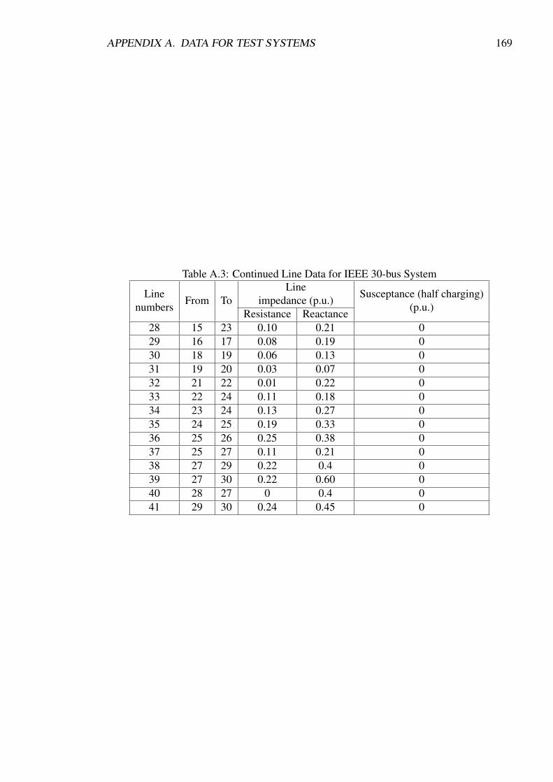
APPENDIX A. DATA FOR TEST SYSTEMS 169
Table A.3: Continued Line Data for IEEE 30-bus System
Linenumbers
From ToLine
impedance (p.u.) Susceptance (half charging)(p.u.)Resistance Reactance
28 15 23 0.10 0.21 029 16 17 0.08 0.19 030 18 19 0.06 0.13 031 19 20 0.03 0.07 032 21 22 0.01 0.22 033 22 24 0.11 0.18 034 23 24 0.13 0.27 035 24 25 0.19 0.33 036 25 26 0.25 0.38 037 25 27 0.11 0.21 038 27 29 0.22 0.4 039 27 30 0.22 0.60 040 28 27 0 0.4 041 29 30 0.24 0.45 0