distributed-memory programming with mpi 3 - elsevier · 2013-12-20 · 84 chapter 3...
TRANSCRIPT

CHAPTER
3Distributed-MemoryProgramming with MPI
Recall that the world of parallel multiple instruction, multiple data, or MIMD, com-puters is, for the most part, divided into distributed-memory and shared-memorysystems. From a programmer’s point of view, a distributed-memory system consistsof a collection of core-memory pairs connected by a network, and the memory asso-ciated with a core is directly accessible only to that core. See Figure 3.1. On the otherhand, from a programmer’s point of view, a shared-memory system consists of a col-lection of cores connected to a globally accessible memory, in which each core canhave access to any memory location. See Figure 3.2. In this chapter we’re going tostart looking at how to program distributed-memory systems using message-passing.
Recall that in message-passing programs, a program running on one core-memorypair is usually called a process, and two processes can communicate by calling func-tions: one process calls a send function and the other calls a receive function. Theimplementation of message-passing that we’ll be using is called MPI, which is anabbreviation of Message-Passing Interface. MPI is not a new programming lan-guage. It defines a library of functions that can be called from C, C++, and Fortranprograms. We’ll learn about some of MPI’s different send and receive functions.We’ll also learn about some “global” communication functions that can involve morethan two processes. These functions are called collective communications. In the pro-cess of learning about all of these MPI functions, we’ll also learn about some of the
CPU
Memory
CPU
Memory
CPU
Memory
CPU
Memory
Interconnect
FIGURE 3.1
A distributed-memory system
An Introduction to Parallel ProgrammingCopyright c© 2011 Elsevier Inc. All rights reserved.
83

84 CHAPTER 3 Distributed-Memory Programming with MPI
Interconnect
CPU CPU CPU CPU
Memory
FIGURE 3.2
A shared-memory system
fundamental issues involved in writing message-passing programs–issues such asdata partitioning and I/O in distributed-memory systems. We’ll also revisit the issueof parallel program performance.
3.1 GETTING STARTEDPerhaps the first program that many of us saw was some variant of the “hello, world”program in Kernighan and Ritchie’s classic text [29]:
#include <stdio.h>
int main(void) {printf("hello, world\n");
return 0;}
Let’s write a program similar to “hello, world” that makes some use of MPI. Insteadof having each process simply print a message, we’ll designate one process to do theoutput, and the other processes will send it messages, which it will print.
In parallel programming, it’s common (one might say standard) for the processesto be identified by nonnegative integer ranks. So if there are p processes, the pro-cesses will have ranks 0,1,2, . . . , p− 1. For our parallel “hello, world,” let’s makeprocess 0 the designated process, and the other processes will send it messages. SeeProgram 3.1.
3.1.1 Compilation and executionThe details of compiling and running the program depend on your system, so youmay need to check with a local expert. However, recall that when we need to beexplicit, we’ll assume that we’re using a text editor to write the program source, and

3.1 Getting Started 85
1 #include <stdio.h>2 #include <string.h> /∗ For strlen ∗/3 #include <mpi.h> /∗ For MPI functions, etc ∗/45 const int MAX STRING = 100;67 int main(void) {8 char greeting[MAX STRING];9 int comm sz; /∗ Number of processes ∗/
10 int my rank; /∗ My process rank ∗/1112 MPI Init(NULL, NULL);13 MPI Comm size(MPI COMM WORLD, &comm sz);14 MPI Comm rank(MPI COMM WORLD, &my rank);1516 if (my rank != 0) {17 sprintf(greeting, "Greetings from process %d of %d!",18 my rank, comm sz);19 MPI Send(greeting, strlen(greeting)+1, MPI CHAR, 0, 0,20 MPI COMM WORLD);21 } else {22 printf("Greetings from process %d of %d!\n", my rank,
comm sz);23 for (int q = 1; q < comm sz; q++) {24 MPI Recv(greeting, MAX STRING, MPI CHAR, q,25 0, MPI COMM WORLD, MPI STATUS IGNORE);26 printf("%s\n", greeting);27 }
28 }
2930 MPI Finalize();31 return 0;32 } /∗ main ∗/
Program 3.1: MPI program that prints greetings from the processes
the command line to compile and run. Many systems use a command called mpiccfor compilation:1
$ mpicc −g −Wall −o mpi hello mpi hello.c
Typically, mpicc is a script that’s a wrapper for the C compiler. A wrapper scriptis a script whose main purpose is to run some program. In this case, the programis the C compiler. However, the wrapper simplifies the running of the compiler bytelling it where to find the necessary header files and which libraries to link with theobject file.
1Recall that the dollar sign ($) is the shell prompt, so it shouldn’t be typed in. Also recall that, forthe sake of explicitness, we assume that we’re using the Gnu C compiler, gcc, and we always use theoptions -g, -Wall, and -o. See Section 2.9 for further information.

86 CHAPTER 3 Distributed-Memory Programming with MPI
Many systems also support program startup with mpiexec:
$ mpiexec −n <number of processes> ./mpi hello
So to run the program with one process, we’d type
$ mpiexec −n 1 ./mpi hello
and to run the program with four processes, we’d type
$ mpiexec −n 4 ./mpi hello
With one process the program’s output would be
Greetings from process 0 of 1!
and with four processes the program’s output would be
Greetings from process 0 of 4!Greetings from process 1 of 4!Greetings from process 2 of 4!Greetings from process 3 of 4!
How do we get from invoking mpiexec to one or more lines of greetings? Thempiexec command tells the system to start <number of processes> instances ofour <mpi hello> program. It may also tell the system which core should run eachinstance of the program. After the processes are running, the MPI implementationtakes care of making sure that the processes can communicate with each other.
3.1.2 MPI programsLet’s take a closer look at the program. The first thing to observe is that this is a Cprogram. For example, it includes the standard C header files stdio.h and string.h.It also has a main function just like any other C program. However, there are manyparts of the program which are new. Line 3 includes the mpi.h header file. Thiscontains prototypes of MPI functions, macro definitions, type definitions, and so on;it contains all the definitions and declarations needed for compiling an MPI program.
The second thing to observe is that all of the identifiers defined by MPI start withthe string MPI . The first letter following the underscore is capitalized for functionnames and MPI-defined types. All of the letters in MPI-defined macros and con-stants are capitalized, so there’s no question about what is defined by MPI and what’sdefined by the user program.
3.1.3 MPI Init and MPI FinalizeIn Line 12 the call to MPI Init tells the MPI system to do all of the necessary setup.For example, it might allocate storage for message buffers, and it might decide whichprocess gets which rank. As a rule of thumb, no other MPI functions should be calledbefore the program calls MPI Init. Its syntax is

3.1 Getting Started 87
int MPI Init(int∗ argc p /∗ in/out ∗/,char∗∗∗ argv p /∗ in/out ∗/);
The arguments, argc p and argv p, are pointers to the arguments to main, argc, andargv. However, when our program doesn’t use these arguments, we can just passNULL for both. Like most MPI functions, MPI Init returns an int error code, and inmost cases we’ll ignore these error codes.
In Line 30 the call to MPI Finalize tells the MPI system that we’re done usingMPI, and that any resources allocated for MPI can be freed. The syntax is quitesimple:
int MPI Finalize(void);
In general, no MPI functions should be called after the call to MPI Finalize.Thus, a typical MPI program has the following basic outline:
. . .#include <mpi.h>. . .int main(int argc, char∗ argv[]) {
. . ./∗ No MPI calls before this ∗/MPI Init(&argc, &argv);. . .MPI Finalize();/∗ No MPI calls after this ∗/. . .return 0;
}
However, we’ve already seen that it’s not necessary to pass pointers to argc and argvto MPI Init. It’s also not necessary that the calls to MPI Init and MPI Finalize bein main.
3.1.4 Communicators, MPI Comm size and MPI Comm rankIn MPI a communicator is a collection of processes that can send messages to eachother. One of the purposes of MPI Init is to define a communicator that consists ofall of the processes started by the user when she started the program. This commu-nicator is called MPI COMM WORLD. The function calls in Lines 13 and 14 are gettinginformation about MPI COMM WORLD. Their syntax is
int MPI Comm size(MPI Comm comm /∗ in ∗/,int∗ comm sz p /∗ out ∗/);
int MPI Comm rank(MPI Comm comm /∗ in ∗/,int∗ my rank p /∗ out ∗/);

88 CHAPTER 3 Distributed-Memory Programming with MPI
For both functions, the first argument is a communicator and has the special typedefined by MPI for communicators, MPI Comm. MPI Comm size returns in its secondargument the number of processes in the communicator, and MPI Comm rank returnsin its second argument the calling process’ rank in the communicator. We’ll oftenuse the variable comm sz for the number of processes in MPI COMM WORLD, and thevariable my rank for the process rank.
3.1.5 SPMD programsNotice that we compiled a single program—we didn’t compile a different programfor each process—and we did this in spite of the fact that process 0 is doing somethingfundamentally different from the other processes: it’s receiving a series of messagesand printing them, while each of the other processes is creating and sending a mes-sage. This is quite common in parallel programming. In fact, most MPI programsare written in this way. That is, a single program is written so that different processescarry out different actions, and this is achieved by simply having the processes branchon the basis of their process rank. Recall that this approach to parallel programming iscalled single program, multiple data, or SPMD. The if−else statement in Lines 16through 28 makes our program SPMD.
Also notice that our program will, in principle, run with any number of processes.We saw a little while ago that it can be run with one process or four processes, but ifour system has sufficient resources, we could also run it with 1000 or even 100,000processes. Although MPI doesn’t require that programs have this property, it’s almostalways the case that we try to write programs that will run with any number of pro-cesses, because we usually don’t know in advance the exact resources available tous. For example, we might have a 20-core system available today, but tomorrow wemight have access to a 500-core system.
3.1.6 CommunicationIn Lines 17 and 18, each process, other than process 0, creates a message it willsend to process 0. (The function sprintf is very similar to printf, except thatinstead of writing to stdout, it writes to a string.) Lines 19–20 actually send themessage to process 0. Process 0, on the other hand, simply prints its message usingprintf, and then uses a for loop to receive and print the messages sent by pro-cesses 1,2, . . . ,comm sz− 1. Lines 24–25 receive the message sent by process q, forq= 1,2, . . . ,comm sz− 1.
3.1.7 MPI SendThe sends executed by processes 1,2, . . . ,comm sz− 1 are fairly complex, so let’stake a closer look at them. Each of the sends is carried out by a call to MPI Send,whose syntax is

3.1 Getting Started 89
int MPI Send(void∗ msg buf p /∗ in ∗/,int msg size /∗ in ∗/,MPI Datatype msg type /∗ in ∗/,int dest /∗ in ∗/,int tag /∗ in ∗/,MPI Comm communicator /∗ in ∗/);
The first three arguments, msg buf p, msg size, and msg type, determine the con-tents of the message. The remaining arguments, dest, tag, and communicator,determine the destination of the message.
The first argument, msg buf p, is a pointer to the block of memory containingthe contents of the message. In our program, this is just the string containing themessage, greeting. (Remember that in C an array, such as a string, is a pointer.)The second and third arguments, msg size and msg type, determine the amount ofdata to be sent. In our program, the msg size argument is the number of characters inthe message plus one character for the ‘\0’ character that terminates C strings. Themsg type argument is MPI CHAR. These two arguments together tell the system thatthe message contains strlen(greeting)+1 chars.
Since C types (int, char, and so on.) can’t be passed as arguments to functions,MPI defines a special type, MPI Datatype, that is used for the msg type argument.MPI also defines a number of constant values for this type. The ones we’ll use (and afew others) are listed in Table 3.1.
Notice that the size of the string greeting is not the same as the size of the mes-sage specified by the arguments msg size and msg type. For example, when we runthe program with four processes, the length of each of the messages is 31 characters,
Table 3.1 Some Predefined MPIDatatypes
MPI datatype C datatype
MPI CHAR signed charMPI SHORT signed short intMPI INT signed intMPI LONG signed long intMPI LONG LONG signed long long intMPI UNSIGNED CHAR unsigned charMPI UNSIGNED SHORT unsigned short intMPI UNSIGNED unsigned intMPI UNSIGNED LONG unsigned long intMPI FLOAT floatMPI DOUBLE doubleMPI LONG DOUBLE long doubleMPI BYTEMPI PACKED

90 CHAPTER 3 Distributed-Memory Programming with MPI
while we’ve allocated storage for 100 characters in greetings. Of course, the sizeof the message sent should be less than or equal to the amount of storage in thebuffer—in our case the string greeting.
The fourth argument, dest, specifies the rank of the process that should receivethe message. The fifth argument, tag, is a nonnegative int. It can be used to dis-tinguish messages that are otherwise identical. For example, suppose process 1 issending floats to process 0. Some of the floats should be printed, while others shouldbe used in a computation. Then the first four arguments to MPI Send provide noinformation regarding which floats should be printed and which should be used in acomputation. So process 1 can use, say, a tag of 0 for the messages that should beprinted and a tag of 1 for the messages that should be used in a computation.
The final argument to MPI Send is a communicator. All MPI functions that involvecommunication have a communicator argument. One of the most important purposesof communicators is to specify communication universes; recall that a communica-tor is a collection of processes that can send messages to each other. Conversely, amessage sent by a process using one communicator cannot be received by a processthat’s using a different communicator. Since MPI provides functions for creating newcommunicators, this feature can be used in complex programs to insure that messagesaren’t “accidentally received” in the wrong place.
An example will clarify this. Suppose we’re studying global climate change, andwe’ve been lucky enough to find two libraries of functions, one for modeling theEarth’s atmosphere and one for modeling the Earth’s oceans. Of course, both librariesuse MPI. These models were built independently, so they don’t communicate witheach other, but they do communicate internally. It’s our job to write the interfacecode. One problem we need to solve is to insure that the messages sent by one librarywon’t be accidentally received by the other. We might be able to work out somescheme with tags: the atmosphere library gets tags 0,1, . . . ,n− 1 and the ocean librarygets tags n,n+ 1, . . . ,n+m. Then each library can use the given range to figure outwhich tag it should use for which message. However, a much simpler solution isprovided by communicators: we simply pass one communicator to the atmospherelibrary functions and a different communicator to the ocean library functions.
3.1.8 MPI RecvThe first six arguments to MPI Recv correspond to the first six arguments ofMPI Send:
int MPI Recv(void∗ msg buf p /∗ out ∗/,int buf size /∗ in ∗/,MPI Datatype buf type /∗ in ∗/,int source /∗ in ∗/,int tag /∗ in ∗/,MPI Comm communicator /∗ in ∗/,MPI Status∗ status p /∗ out ∗/);
Thus, the first three arguments specify the memory available for receiving themessage: msg buf p points to the block of memory, buf size determines the
3.1 Getting Started 91
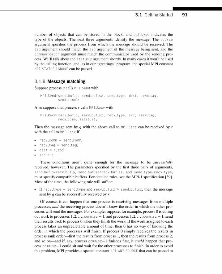
number of objects that can be stored in the block, and buf type indicates thetype of the objects. The next three arguments identify the message. The sourceargument specifies the process from which the message should be received. Thetag argument should match the tag argument of the message being sent, and thecommunicator argument must match the communicator used by the sending pro-cess. We’ll talk about the status p argument shortly. In many cases it won’t be usedby the calling function, and, as in our “greetings” program, the special MPI constantMPI STATUS IGNORE can be passed.
3.1.9 Message matchingSuppose process q calls MPI Send with
MPI Send(send buf p, send buf sz, send type, dest, send tag,send comm);
Also suppose that process r calls MPI Recv with
MPI Recv(recv buf p, recv buf sz, recv type, src, recv tag,recv comm, &status);
Then the message sent by q with the above call to MPI Send can be received by rwith the call to MPI Recv if
. recv comm = send comm,. recv tag = send tag,. dest = r, and. src = q.
These conditions aren’t quite enough for the message to be successfullyreceived, however. The parameters specified by the first three pairs of arguments,send buf p/recv buf p, send buf sz/recv buf sz, and send type/recv type,must specify compatible buffers. For detailed rules, see the MPI-1 specification [39].Most of the time, the following rule will suffice:
. If recv type = send type and recv buf sz ≥ send buf sz, then the messagesent by q can be successfully received by r.
Of course, it can happen that one process is receiving messages from multipleprocesses, and the receiving process doesn’t know the order in which the other pro-cesses will send the messages. For example, suppose, for example, process 0 is dolingout work to processes 1,2, . . . ,comm sz− 1, and processes 1,2, . . . ,comm sz− 1, sendtheir results back to process 0 when they finish the work. If the work assigned to eachprocess takes an unpredictable amount of time, then 0 has no way of knowing theorder in which the processes will finish. If process 0 simply receives the results inprocess rank order—first the results from process 1, then the results from process 2,and so on—and if, say, process comm sz−1 finishes first, it could happen that pro-cess comm sz−1 could sit and wait for the other processes to finish. In order to avoidthis problem, MPI provides a special constant MPI ANY SOURCE that can be passed to

92 CHAPTER 3 Distributed-Memory Programming with MPI
MPI Recv. Then, if process 0 executes the following code, it can receive the resultsin the order in which the processes finish:
for (i = 1; i < comm sz; i++) {MPI Recv(result, result sz, result type, MPI ANY SOURCE,
result tag, comm, MPI STATUS IGNORE);Process result(result);
}
Similarly, it’s possible that one process can be receiving multiple messages withdifferent tags from another process, and the receiving process doesn’t know the orderin which the messages will be sent. For this circumstance, MPI provides the specialconstant MPI ANY TAG that can be passed to the tag argument of MPI Recv.
A couple of points should be stressed in connection with these “wildcard”arguments:
1. Only a receiver can use a wildcard argument. Senders must specify a processrank and a nonnegative tag. Thus, MPI uses a “push” communication mechanismrather than a “pull” mechanism.
2. There is no wildcard for communicator arguments; both senders and receiversmust always specify communicators.
3.1.10 The status p argumentIf you think about these rules for a minute, you’ll notice that a receiver can receive amessage without knowing
1. the amount of data in the message,2. the sender of the message, or3. the tag of the message.
So how can the receiver find out these values? Recall that the last argument toMPI Recv has type MPI Status∗. The MPI type MPI Status is a struct with at leastthe three members MPI SOURCE, MPI TAG, and MPI ERROR. Suppose our programcontains the definition
MPI Status status;
Then, after a call to MPI Recv in which &status is passed as the last argument, wecan determine the sender and tag by examining the two members
status.MPI SOURCEstatus.MPI TAG
The amount of data that’s been received isn’t stored in a field that’s directlyaccessible to the application program. However, it can be retrieved with a call toMPI Get count. For example, suppose that in our call to MPI Recv, the type of thereceive buffer is recv type and, once again, we passed in &status. Then the call
MPI Get count(&status, recv type, &count)
3.1 Getting Started 93
will return the number of elements received in the count argument. In general, thesyntax of MPI Get count is
int MPI Get count(MPI Status∗ status p /∗ in ∗/,MPI Datatype type /∗ in ∗/,int∗ count p /∗ out ∗/);
Note that the count isn’t directly accessible as a member of the MPI Statusvariable simply because it depends on the type of the received data, and, conse-quently, determining it would probably require a calculation (e.g. (number of bytesreceived)/(bytes per object)). If this information isn’t needed, we shouldn’t waste acalculation determining it.
3.1.11 Semantics of MPI Send and MPI RecvWhat exactly happens when we send a message from one process to another? Manyof the details depend on the particular system, but we can make a few generaliza-tions. The sending process will assemble the message. For example, it will add the“envelope” information to the actual data being transmitted—the destination processrank, the sending process rank, the tag, the communicator, and some informationon the size of the message. Once the message has been assembled, recall fromChapter 2 that there are essentially two possibilities: the sending process can bufferthe message or it can block. If it buffers the message, the MPI system will place themessage (data and envelope) into its own internal storage, and the call to MPI Sendwill return.
Alternatively, if the system blocks, it will wait until it can begin transmittingthe message, and the call to MPI Send may not return immediately. Thus, if we useMPI Send, when the function returns, we don’t actually know whether the messagehas been transmitted. We only know that the storage we used for the message, thesend buffer, is available for reuse by our program. If we need to know that themessage has been transmitted, or if we need for our call to MPI Send to returnimmediately—regardless of whether the message has been sent—MPI provides alter-native functions for sending. We’ll learn about one of these alternative functionslater.
The exact behavior of MPI Send is determined by the MPI implementation. How-ever, typical implementations have a default “cutoff” message size. If the size of amessage is less than the cutoff, it will be buffered. If the size of the message is greaterthan the cutoff, MPI Send will block.
Unlike MPI Send, MPI Recv always blocks until a matching message has beenreceived. Thus, when a call to MPI Recv returns, we know that there is a messagestored in the receive buffer (unless there’s been an error). There is an alternate methodfor receiving a message, in which the system checks whether a matching message isavailable and returns, regardless of whether there is one. (For more details on the useof nonblocking communication, see Exercise 6.22.)
MPI requires that messages be nonovertaking. This means that if process q sendstwo messages to process r, then the first message sent by q must be available to r

94 CHAPTER 3 Distributed-Memory Programming with MPI
before the second message. However, there is no restriction on the arrival of mes-sages sent from different processes. That is, if q and t both send messages to r,then even if q sends its message before t sends its message, there is no require-ment that q’s message become available to r before t’s message. This is essentiallybecause MPI can’t impose performance on a network. For example, if q happensto be running on a machine on Mars, while r and t are both running on the samemachine in San Francisco, and if q sends its message a nanosecond before t sendsits message, it would be extremely unreasonable to require that q’s message arrivebefore t’s.
3.1.12 Some potential pitfallsNote that the semantics of MPI Recv suggests a potential pitfall in MPI programming:If a process tries to receive a message and there’s no matching send, then the processwill block forever. That is, the process will hang. When we design our programs, wetherefore need to be sure that every receive has a matching send. Perhaps even moreimportant, we need to be very careful when we’re coding that there are no inadvertentmistakes in our calls to MPI Send and MPI Recv. For example, if the tags don’t match,or if the rank of the destination process is the same as the rank of the source process,the receive won’t match the send, and either a process will hang, or, perhaps worse,the receive may match another send.
Similarly, if a call to MPI Send blocks and there’s no matching receive, then thesending process can hang. If, on the other hand, a call to MPI Send is buffered andthere’s no matching receive, then the message will be lost.
3.2 THE TRAPEZOIDAL RULE IN MPIPrinting messages from processes is all well and good, but we’re probably not tak-ing the trouble to learn to write MPI programs just to print messages. Let’s take alook at a somewhat more useful program—let’s write a program that implements thetrapezoidal rule for numerical integration.
3.2.1 The trapezoidal ruleRecall that we can use the trapezoidal rule to approximate the area between the graphof a function, y= f (x), two vertical lines, and the x-axis. See Figure 3.3. The basicidea is to divide the interval on the x-axis into n equal subintervals. Then we approxi-mate the area lying between the graph and each subinterval by a trapezoid whose baseis the subinterval, whose vertical sides are the vertical lines through the endpoints ofthe subinterval, and whose fourth side is the secant line joining the points where thevertical lines cross the graph. See Figure 3.4. If the endpoints of the subinterval arexi and xi+1, then the length of the subinterval is h= xi+1− xi. Also, if the lengths ofthe two vertical segments are f (xi) and f (xi+1), then the area of the trapezoid is
Area of one trapezoid =h
2[ f (xi)+ f (xi+1)].

3.2 The Trapezoidal Rule in MPI 95
y
a b x a b
y
x
(a) (b)
FIGURE 3.3
The trapezoidal rule: (a) area to be estimated and (b) approximate area using trapezoids
Since we chose the n subintervals so that they would all have the same length, wealso know that if the vertical lines bounding the region are x= a and x= b, then
h=b− a
n.
Thus, if we call the leftmost endpoint x0, and the rightmost endpoint xn, we have
x0 = a, x1 = a+ h, x2 = a+ 2h, . . . , xn−1 = a+ (n− 1)h, xn = b,
and the sum of the areas of the trapezoids—our approximation to the total area—is
Sum of trapezoid areas = h[ f (x0)/2+ f (x1)+ f (x2)+ ·· ·+ f (xn−1)+ f (xn)/2].
Thus, pseudo-code for a serial program might look something like this:
/∗ Input: a, b, n ∗/h = (b−a)/n;approx = (f(a) + f(b))/2.0;for (i = 1; i <= n−1; i++) {
x i = a + i∗h;approx += f(x i);
}
approx = h∗approx;
y
f (xi)y = f (x)
f (xi+1)
x
h
xi xi+1
FIGURE 3.4
One trapezoid

96 CHAPTER 3 Distributed-Memory Programming with MPI
3.2.2 Parallelizing the trapezoidal ruleIt is not the most attractive word, but, as we noted in Chapter 1, people who writeparallel programs do use the verb “parallelize” to describe the process of convertinga serial program or algorithm into a parallel program.
Recall that we can design a parallel program using four basic steps:
1. Partition the problem solution into tasks.2. Identify the communication channels between the tasks.3. Aggregate the tasks into composite tasks.4. Map the composite tasks to cores.
In the partitioning phase, we usually try to identify as many tasks as possible. For thetrapezoidal rule, we might identify two types of tasks: one type is finding the areaof a single trapezoid, and the other is computing the sum of these areas. Then thecommunication channels will join each of the tasks of the first type to the single taskof the second type. See Figure 3.5.
So how can we aggregate the tasks and map them to the cores? Our intuition tellsus that the more trapezoids we use, the more accurate our estimate will be. That is,we should use many trapezoids, and we will use many more trapezoids than cores.Thus, we need to aggregate the computation of the areas of the trapezoids into groups.A natural way to do this is to split the interval [a,b] up into comm sz subintervals. Ifcomm sz evenly divides n, the number of trapezoids, we can simply apply the trape-zoidal rule with n/comm sz trapezoids to each of the comm sz subintervals. To finish,we can have one of the processes, say process 0, add the estimates.
Let’s make the simplifying assumption that comm sz evenly divides n. Thenpseudo-code for the program might look something like the following:
1 Get a, b, n;2 h = (b−a)/n;3 local n = n/comm sz;4 local a = a + my rank∗local n∗h;5 local b = local a + local n∗h;6 local integral = Trap(local a, local b, local n, h);
Add areas
Compute areaof trap 0
Compute areaof trap 1
Compute areaof trap n − 1
FIGURE 3.5
Tasks and communications for the trapezoidal rule

3.3 Dealing with I/O 97
7 if (my rank != 0)8 Send local integral to process 0;9 else /∗ my rank == 0 ∗/
10 total integral = local integral;11 for (proc = 1; proc < comm sz; proc++) {12 Receive local integral from proc;13 total integral += local integral;14 }
15 }
16 if (my rank == 0)17 print result;
Let’s defer, for the moment, the issue of input and just “hardwire” the values for a,b, and n. When we do this, we get the MPI program shown in Program 3.2. The Trapfunction is just an implementation of the serial trapezoidal rule. See Program 3.3.
Notice that in our choice of identifiers, we try to differentiate between local andglobal variables. Local variables are variables whose contents are significant only onthe process that’s using them. Some examples from the trapezoidal rule program arelocal a, local b, and local n. Variables whose contents are significant to all theprocesses are sometimes called global variables. Some examples from the trapezoidalrule are a, b, and n. Note that this usage is different from the usage you learned in yourintroductory programming class, where local variables are private to a single functionand global variables are accessible to all the functions. However, no confusion shouldarise, since the context will usually make the meaning clear.
3.3 DEALING WITH I/OOf course, the current version of the parallel trapezoidal rule has a serious deficiency:it will only compute the integral over the interval [0,3] using 1024 trapezoids. We canedit the code and recompile, but this is quite a bit of work compared to simply typingin three new numbers. We need to address the problem of getting input from the user.While we’re talking about input to parallel programs, it might be a good idea to alsotake a look at output. We discussed these two issues in Chapter 2, so if you rememberthe discussion of nondeterminism and output, you can skip ahead to Section 3.3.2.
3.3.1 OutputIn both the “greetings” program and the trapezoidal rule program we’ve assumedthat process 0 can write to stdout, that is, its calls to printf behave as we mightexpect. Although the MPI standard doesn’t specify which processes have accessto which I/O devices, virtually all MPI implementations allow all the processes inMPI COMM WORLD full access to stdout and stderr, so most MPI implementationsallow all processes to execute printf and fprintf(stderr, ...).
However, most MPI implementations don’t provide any automatic scheduling ofaccess to these devices. That is, if multiple processes are attempting to write to,

98 CHAPTER 3 Distributed-Memory Programming with MPI
1 int main(void) {2 int my rank, comm sz, n = 1024, local n;3 double a = 0.0, b = 3.0, h, local a, local b;4 double local int, total int;5 int source;67 MPI Init(NULL, NULL);8 MPI Comm rank(MPI COMM WORLD, &my rank);9 MPI Comm size(MPI COMM WORLD, &comm sz);
1011 h = (b−a)/n; /∗ h is the same for all processes ∗/12 local n = n/comm sz; /∗ So is the number of trapezoids ∗/1314 local a = a + my rank∗local n∗h;15 local b = local a + local n∗h;16 local int = Trap(local a, local b, local n, h);1718 if (my rank != 0) {19 MPI Send(&local int, 1, MPI DOUBLE, 0, 0,20 MPI COMM WORLD);21 } else {22 total int = local int;23 for (source = 1; source < comm sz; source++) {24 MPI Recv(&local int, 1, MPI DOUBLE, source, 0,25 MPI COMM WORLD, MPI STATUS IGNORE);26 total int += local int;27 }
28 }
2930 if (my rank == 0) {31 printf("With n = %d trapezoids, our estimate\n", n);32 printf("of the integral from %f to %f = %.15e\n",33 a, b, total int);34 }
35 MPI Finalize();36 return 0;37 } /∗ main ∗/
Program 3.2: First version of the MPI trapezoidal rule
say, stdout, the order in which the processes’ output appears will be unpredictable.Indeed, it can even happen that the output of one process will be interrupted by theoutput of another process.
For example, suppose we try to run an MPI program in which each process simplyprints a message. See Program 3.4. On our cluster, if we run the program with fiveprocesses, it often produces the “expected” output:
Proc 0 of 5 > Does anyone have a toothpick?Proc 1 of 5 > Does anyone have a toothpick?Proc 2 of 5 > Does anyone have a toothpick?

3.3 Dealing with I/O 99
1 double Trap(2 double left endpt /∗ in ∗/,3 double right endpt /∗ in ∗/,4 int trap count /∗ in ∗/,5 double base len /∗ in ∗/) {6 double estimate, x;7 int i;89 estimate = (f(left endpt) + f(right endpt))/2.0;
10 for (i = 1; i <= trap count−1; i++) {11 x = left endpt + i∗base len;12 estimate += f(x);13 }
14 estimate = estimate∗base len;1516 return estimate;17 } /∗ Trap ∗/
Program 3.3: Trap function in the MPI trapezoidal rule
#include <stdio.h>#include <mpi.h>
int main(void) {int my rank, comm sz;
MPI Init(NULL, NULL);MPI Comm size(MPI COMM WORLD, &comm sz);MPI Comm rank(MPI COMM WORLD, &my rank);
printf("Proc %d of %d > Does anyone have a toothpick?\n",my rank, comm sz);
MPI Finalize();return 0;
} /∗ main ∗/
Program 3.4: Each process just prints a message
Proc 3 of 5 > Does anyone have a toothpick?Proc 4 of 5 > Does anyone have a toothpick?
However, when we run it with six processes, the order of the output lines isunpredictable:
Proc 0 of 6 > Does anyone have a toothpick?Proc 1 of 6 > Does anyone have a toothpick?Proc 2 of 6 > Does anyone have a toothpick?

100 CHAPTER 3 Distributed-Memory Programming with MPI
Proc 5 of 6 > Does anyone have a toothpick?Proc 3 of 6 > Does anyone have a toothpick?Proc 4 of 6 > Does anyone have a toothpick?
or
Proc 0 of 6 > Does anyone have a toothpick?Proc 1 of 6 > Does anyone have a toothpick?Proc 2 of 6 > Does anyone have a toothpick?Proc 4 of 6 > Does anyone have a toothpick?Proc 3 of 6 > Does anyone have a toothpick?Proc 5 of 6 > Does anyone have a toothpick?
The reason this happens is that the MPI processes are “competing” for access tothe shared output device, stdout, and it’s impossible to predict the order in which theprocesses’ output will be queued up. Such a competition results in nondeterminism.That is, the actual output will vary from one run to the next.
In any case, if we don’t want output from different processes to appear in a randomorder, it’s up to us to modify our program accordingly. For example, we can have eachprocess other than 0 send its output to process 0, and process 0 can print the outputin process rank order. This is exactly what we did in the “greetings” program.
3.3.2 InputUnlike output, most MPI implementations only allow process 0 in MPI COMM WORLDaccess to stdin. This makes sense: If multiple processes have access to stdin, whichprocess should get which parts of the input data? Should process 0 get the first line?Process 1 the second? Or should process 0 get the first character?
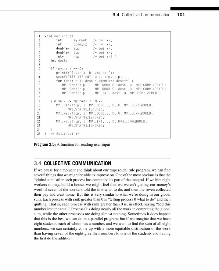
In order to write MPI programs that can use scanf, we need to branch onprocess rank, with process 0 reading in the data and then sending it to the otherprocesses. For example, we might write the Get input function shown in Pro-gram 3.5 for our parallel trapezoidal rule program. In this function, process 0 simplyreads in the values for a, b, and n and sends all three values to each process. Thisfunction uses the same basic communication structure as the “greetings” program,except that now process 0 is sending to each process, while the other processes arereceiving.
To use this function, we can simply insert a call to it inside our main function,being careful to put it after we’ve initialized my rank and comm sz:
. . .MPI Comm rank(MPI COMM WORLD, &my rank);MPI Comm size(MPI COMM WORLD, &comm sz);
Get data(my rank, comm sz, &a, &b, &n);
h = (b−a)/n;. . .
3.4 Collective Communication 101
1 void Get input(2 int my rank /∗ in ∗/,3 int comm sz /∗ in ∗/,4 double∗ a p /∗ out ∗/,5 double∗ b p /∗ out ∗/,6 int∗ n p /∗ out ∗/) {7 int dest;89 if (my rank == 0) {
10 printf("Enter a, b, and n\n");11 scanf("%lf %lf %d", a p, b p, n p);12 for (dest = 1; dest < comm sz; dest++) {13 MPI Send(a p, 1, MPI DOUBLE, dest, 0, MPI COMM WORLD);14 MPI Send(b p, 1, MPI DOUBLE, dest, 0, MPI COMM WORLD);15 MPI Send(n p, 1, MPI INT, dest, 0, MPI COMM WORLD);16 }
17 } else { /∗ my rank != 0 ∗/18 MPI Recv(a p, 1, MPI DOUBLE, 0, 0, MPI COMM WORLD,19 MPI STATUS IGNORE);20 MPI Recv(b p, 1, MPI DOUBLE, 0, 0, MPI COMM WORLD,21 MPI STATUS IGNORE);22 MPI Recv(n p, 1, MPI INT, 0, 0, MPI COMM WORLD,23 MPI STATUS IGNORE);24 }
25 } /∗ Get input ∗/
Program 3.5: A function for reading user input
3.4 COLLECTIVE COMMUNICATIONIf we pause for a moment and think about our trapezoidal rule program, we can findseveral things that we might be able to improve on. One of the most obvious is that the“global sum” after each process has computed its part of the integral. If we hire eightworkers to, say, build a house, we might feel that we weren’t getting our money’sworth if seven of the workers told the first what to do, and then the seven collectedtheir pay and went home. But this is very similar to what we’re doing in our globalsum. Each process with rank greater than 0 is “telling process 0 what to do” and thenquitting. That is, each process with rank greater than 0 is, in effect, saying “add thisnumber into the total.” Process 0 is doing nearly all the work in computing the globalsum, while the other processes are doing almost nothing. Sometimes it does happenthat this is the best we can do in a parallel program, but if we imagine that we haveeight students, each of whom has a number, and we want to find the sum of all eightnumbers, we can certainly come up with a more equitable distribution of the workthan having seven of the eight give their numbers to one of the students and havingthe first do the addition.

102 CHAPTER 3 Distributed-Memory Programming with MPI
3.4.1 Tree-structured communicationAs we already saw in Chapter 1 we might use a “binary tree structure” like thatillustrated in Figure 3.6. In this diagram, initially students or processes 1, 3, 5, and7 send their values to processes 0, 2, 4, and 6, respectively. Then processes 0, 2, 4,and 6 add the received values to their original values, and the process is repeatedtwice:
1. a. Processes 2 and 6 send their new values to processes 0 and 4, respectively.b. Processes 0 and 4 add the received values into their new values.
2. a. Process 4 sends its newest value to process 0.b. Process 0 adds the received value to its newest value.
This solution may not seem ideal, since half the processes (1, 3, 5, and 7) aredoing the same amount of work that they did in the original scheme. However, ifyou think about it, the original scheme required comm sz− 1= seven receives andseven adds by process 0, while the new scheme only requires three, and all the otherprocesses do no more than two receives and adds. Furthermore, the new scheme hasa property by which a lot of the work is done concurrently by different processes.For example, in the first phase, the receives and adds by processes 0, 2, 4, and 6 canall take place simultaneously. So, if the processes start at roughly the same time, thetotal time required to compute the global sum will be the time required by process0, that is, three receives and three additions. We’ve thus reduced the overall time bymore than 50%. Furthermore, if we use more processes, we can do even better. Forexample, if comm sz= 1024, then the original scheme requires process 0 to do 1023receives and additions, while it can be shown (Exercise 3.5) that the new schemerequires process 0 to do only 10 receives and additions. This improves the originalscheme by more than a factor of 100!
Processes
5 2 −1
−4 −5
−3 6 5 −7 2
0 1
7
3
9
6
11
2 3 4 5 6 7
FIGURE 3.6
A tree-structured global sum

3.4 Collective Communication 103
Processes
5 2 −1
−8 −1
−3 6 5 −7 2
0 1
11 7
3 6
9
2 3 4 5 6 7
FIGURE 3.7
An alternative tree-structured global sum
You may be thinking to yourself, this is all well and good, but coding this tree-structured global sum looks like it would take a quite a bit of work, and you’d beright. See Programming Assignment 3.3. In fact, the problem may be even harder.For example, it’s perfectly feasible to construct a tree-structured global sum that usesdifferent “process-pairings.” For example, we might pair 0 and 4, 1 and 5, 2 and 6,and 3 and 7 in the first phase. Then we could pair 0 and 2, and 1 and 3 in the second,and 0 and 1 in the final. See Figure 3.7. Of course, there are many other possibilities.How can we decide which is the best? Do we need to code each alternative andevaluate its performance? If we do, is it possible that one method works best for“small” trees, while another works best for “large” trees? Even worse, one approachmight work best on system A, while another might work best on system B.
3.4.2 MPI ReduceWith virtually limitless possibilities, it’s unreasonable to expect each MPI pro-grammer to write an optimal global-sum function, so MPI specifically protectsprogrammers against this trap of endless optimization by requiring that MPI imple-mentations include implementations of global sums. This places the burden ofoptimization on the developer of the MPI implementation, rather than the applica-tion developer. The assumption here is that the developer of the MPI implementationshould know enough about both the hardware and the system software so that she canmake better decisions about implementation details.
Now, a “global-sum function” will obviously require communication. However,unlike the MPI Send-MPI Recv pair, the global-sum function may involve more thantwo processes. In fact, in our trapezoidal rule program it will involve all the processesin MPI COMM WORLD. In MPI parlance, communication functions that involve all theprocesses in a communicator are called collective communications. To distinguish

104 CHAPTER 3 Distributed-Memory Programming with MPI
between collective communications and functions such as MPI Send and MPI Recv,MPI Send and MPI Recv are often called point-to-point communications.
In fact, global sum is just a special case of an entire class of collective communi-cations. For example, it might happen that instead of finding the sum of a collection ofcomm sz numbers distributed among the processes, we want to find the maximum orthe minimum or the product or any one of many other possibilities. MPI generalizedthe global-sum function so that any one of these possibilities can be implementedwith a single function:
int MPI Reduce(void∗ input data p /∗ in ∗/,void∗ output data p /∗ out ∗/,int count /∗ in ∗/,MPI Datatype datatype /∗ in ∗/,MPI Op operator /∗ in ∗/,int dest process /∗ in ∗/,MPI Comm comm /∗ in ∗/);
The key to the generalization is the fifth argument, operator. It has type MPI Op,which is a predefined MPI type like MPI Datatype and MPI Comm. There are a numberof predefined values in this type. See Table 3.2. It’s also possible to define your ownoperators; for details, see the MPI-1 Standard [39].
The operator we want is MPI SUM. Using this value for the operator argument, wecan replace the code in Lines 18 through 28 of Program 3.2 with the single functioncall
MPI Reduce(&local int, &total int, 1, MPI DOUBLE, MPI SUM, 0,MPI COMM WORLD);
One point worth noting is that by using a count argument greater than 1, MPI Reducecan operate on arrays instead of scalars. The following code could thus be used to
Table 3.2 Predefined Reduction Operators in MPI
Operation Value Meaning
MPI MAX MaximumMPI MIN MinimumMPI SUM SumMPI PROD ProductMPI LAND Logical andMPI BAND Bitwise andMPI LOR Logical orMPI BOR Bitwise orMPI LXOR Logical exclusive orMPI BXOR Bitwise exclusive orMPI MAXLOC Maximum and location of maximumMPI MINLOC Minimum and location of minimum

3.4 Collective Communication 105
add a collection of N-dimensional vectors, one per process:
double local x[N], sum[N];. . .MPI Reduce(local x, sum, N, MPI DOUBLE, MPI SUM, 0,
MPI COMM WORLD);
3.4.3 Collective vs. point-to-point communicationsIt’s important to remember that collective communications differ in several waysfrom point-to-point communications:
1. All the processes in the communicator must call the same collective function. Forexample, a program that attempts to match a call to MPI Reduce on one processwith a call to MPI Recv on another process is erroneous, and, in all likelihood, theprogram will hang or crash.
2. The arguments passed by each process to an MPI collective communication mustbe “compatible.” For example, if one process passes in 0 as the dest processand another passes in 1, then the outcome of a call to MPI Reduce is erroneous,and, once again, the program is likely to hang or crash.
3. The output data p argument is only used on dest process. However, allof the processes still need to pass in an actual argument corresponding tooutput data p, even if it’s just NULL.
4. Point-to-point communications are matched on the basis of tags and communica-tors. Collective communications don’t use tags, so they’re matched solely on thebasis of the communicator and the order in which they’re called. As an example,consider the calls to MPI Reduce shown in Table 3.3. Suppose that each pro-cess calls MPI Reduce with operator MPI SUM, and destination process 0. At firstglance, it might seem that after the two calls to MPI Reduce, the value of b will bethree, and the value of d will be six. However, the names of the memory locationsare irrelevant to the matching, of the calls to MPI Reduce. The order of the callswill determine the matching, so the value stored in b will be 1+ 2+ 1= 4, andthe value stored in d will be 2+ 1+ 2= 5.
A final caveat: it might be tempting to call MPI Reduce using the same buffer forboth input and output. For example, if we wanted to form the global sum of x on eachprocess and store the result in x on process 0, we might try calling
MPI Reduce(&x, &x, 1, MPI DOUBLE, MPI SUM, 0, comm);
Table 3.3 Multiple Calls to MPI Reduce
Time Process 0 Process 1 Process 2
0 a = 1; c = 2 a = 1; c = 2 a = 1; c = 2
1 MPI Reduce(&a, &b, ...) MPI Reduce(&c, &d, ...) MPI Reduce(&a, &b, ...)
2 MPI Reduce(&c, &d, ...) MPI Reduce(&a, &b, ...) MPI Reduce(&c, &d, ...)

106 CHAPTER 3 Distributed-Memory Programming with MPI
However, this call is illegal in MPI, so its result will be unpredictable: it might pro-duce an incorrect result, it might cause the program to crash, it might even producea correct result. It’s illegal because it involves aliasing of an output argument. Twoarguments are aliased if they refer to the same block of memory, and MPI prohibitsaliasing of arguments if one of them is an output or input/output argument. This isbecause the MPI Forum wanted to make the Fortran and C versions of MPI as sim-ilar as possible, and Fortran prohibits aliasing. In some instances, MPI provides analternative construction that effectively avoids this restriction. See Section 6.1.9 foran example.
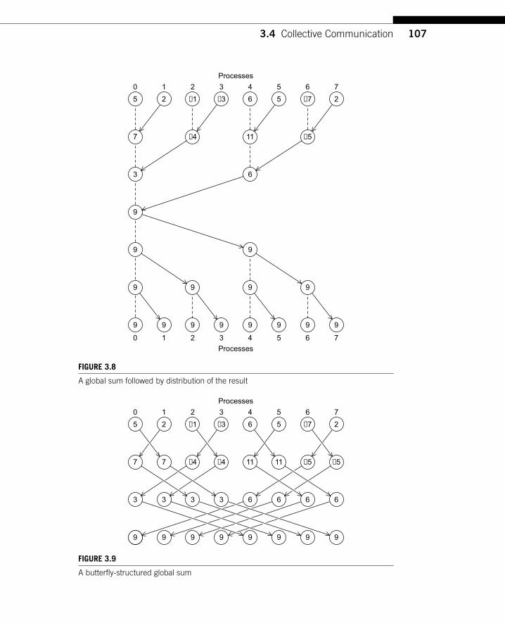
3.4.4 MPI AllreduceIn our trapezoidal rule program, we just print the result, so it’s perfectly natural foronly one process to get the result of the global sum. However, it’s not difficult toimagine a situation in which all of the processes need the result of a global sum inorder to complete some larger computation. In this situation, we encounter some ofthe same problems we encountered with our original global sum. For example, if weuse a tree to compute a global sum, we might “reverse” the branches to distributethe global sum (see Figure 3.8). Alternatively, we might have the processes exchangepartial results instead of using one-way communications. Such a communication pat-tern is sometimes called a butterfly (see Figure 3.9). Once again, we don’t want tohave to decide on which structure to use, or how to code it for optimal performance.Fortunately, MPI provides a variant of MPI Reduce that will store the result on all theprocesses in the communicator:
int MPI Allreduce(void∗ input data p /∗ in ∗/,void∗ output data p /∗ out ∗/,int count /∗ in ∗/,MPI Datatype datatype /∗ in ∗/,MPI Op operator /∗ in ∗/,MPI Comm comm /∗ in ∗/);
The argument list is identical to that for MPI Reduce except that there is nodest process since all the processes should get the result.
3.4.5 BroadcastIf we can improve the performance of the global sum in our trapezoidal rule programby replacing a loop of receives on process 0 with a tree-structured communication,we ought to be able to do something similar with the distribution of the input data.In fact, if we simply “reverse” the communications in the tree-structured global sumin Figure 3.6, we obtain the tree-structured communication shown in Figure 3.10,and we can use this structure to distribute the input data. A collective communicationin which data belonging to a single process is sent to all of the processes in thecommunicator is called a broadcast, and you’ve probably guessed that MPI provides
3.4 Collective Communication 107
Processes
Processes
5 2 −1
−4 −511
−3 6 5 −7 2
0 1
7
3 6
9
9
9
9 9 9 9 9 9 9 9
9 9
9
9
2 3 4 5 6 7
0 1 2 3 4 5 6 7
FIGURE 3.8
A global sum followed by distribution of the result
Processes
5 2 −1
−4 −4 −5 −5
−3 6 5 −7 2
0 1
7 7 11 11
3
9 9 9 9 9 9 9 9
3 3 3 6 6 6 6
2 3 4 5 6 7
FIGURE 3.9
A butterfly-structured global sum
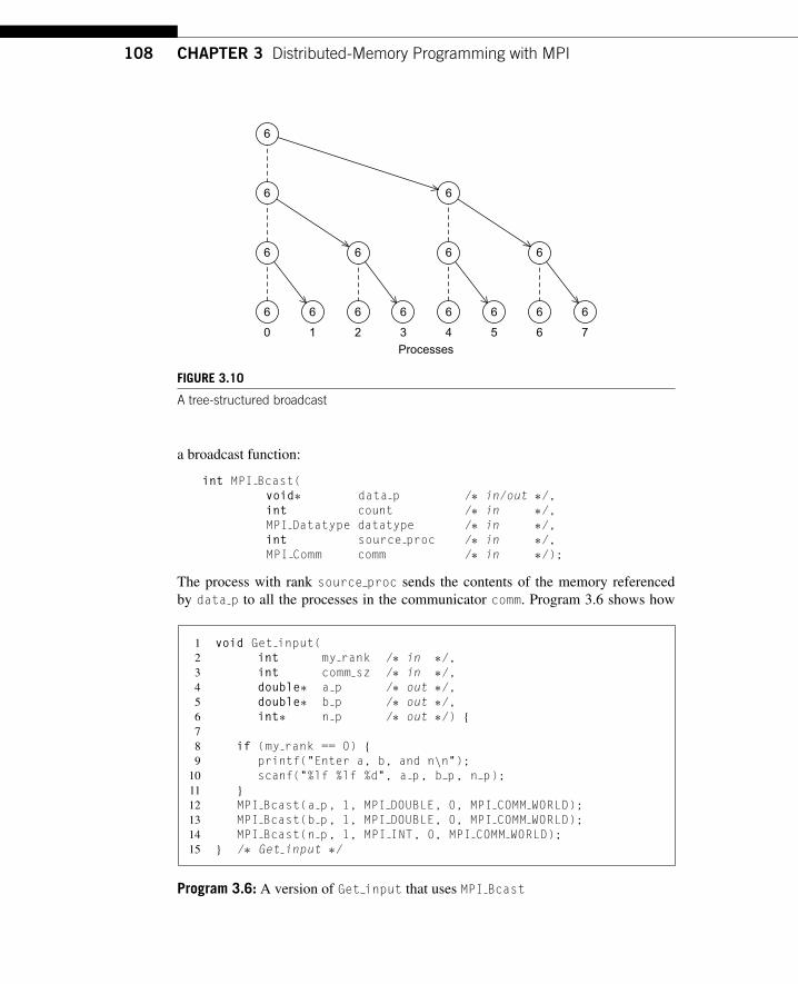
108 CHAPTER 3 Distributed-Memory Programming with MPI
Processes
6
6
6
6 6 6 6 6 6 6 6
6 6
6
6
0 1 2 3 4 5 6 7
FIGURE 3.10
A tree-structured broadcast
a broadcast function:
int MPI Bcast(void∗ data p /∗ in/out ∗/,int count /∗ in ∗/,MPI Datatype datatype /∗ in ∗/,int source proc /∗ in ∗/,MPI Comm comm /∗ in ∗/);
The process with rank source proc sends the contents of the memory referencedby data p to all the processes in the communicator comm. Program 3.6 shows how
1 void Get input(2 int my rank /∗ in ∗/,3 int comm sz /∗ in ∗/,4 double∗ a p /∗ out ∗/,5 double∗ b p /∗ out ∗/,6 int∗ n p /∗ out ∗/) {78 if (my rank == 0) {9 printf("Enter a, b, and n\n");
10 scanf("%lf %lf %d", a p, b p, n p);11 }
12 MPI Bcast(a p, 1, MPI DOUBLE, 0, MPI COMM WORLD);13 MPI Bcast(b p, 1, MPI DOUBLE, 0, MPI COMM WORLD);14 MPI Bcast(n p, 1, MPI INT, 0, MPI COMM WORLD);15 } /∗ Get input ∗/
Program 3.6: A version of Get input that uses MPI Bcast

3.4 Collective Communication 109
to modify the Get input function shown in Program 3.5 so that it uses MPI Bcastinstead of MPI Send and MPI Recv.
Recall that in serial programs, an in/out argument is one whose value is bothused and changed by the function. For MPI Bcast, however, the data p argument isan input argument on the process with rank source proc and an output argumenton the other processes. Thus, when an argument to a collective communication islabeled in/out, it’s possible that it’s an input argument on some processes and anoutput argument on other processes.
3.4.6 Data distributionsSuppose we want to write a function that computes a vector sum:
x+ y= (x0,x1, . . . ,xn−1)+ (y0,y1, . . . ,yn−1)
= (x0+ y0,x1+ y1, . . . ,xn−1+ yn−1)
= (z0,z1, . . . ,zn−1)
= z
If we implement the vectors as arrays of, say, doubles, we could implement serialvector addition with the code shown in Program 3.7.
1 void Vector sum(double x[], double y[], double z[], int n) {2 int i;34 for (i = 0; i < n; i++)5 z[i] = x[i] + y[i];6 } /∗ Vector sum ∗/
Program 3.7: A serial implementation of vector addition
How could we implement this using MPI? The work consists of adding the indi-vidual components of the vectors, so we might specify that the tasks are just theadditions of corresponding components. Then there is no communication betweenthe tasks, and the problem of parallelizing vector addition boils down to aggregat-ing the tasks and assigning them to the cores. If the number of components is n andwe have comm sz cores or processes, let’s assume that n evenly divides comm sz anddefine local n= n/comm sz. Then we can simply assign blocks of local n consec-utive components to each process. The four columns on the left of Table 3.4 show anexample when n= 12 and comm sz= 3. This is often called a block partition of thevector.
An alternative to a block partition is a cyclic partition. In a cyclic partition,we assign the components in a round robin fashion. The four columns in the mid-dle of Table 3.4 show an example when n= 12 and comm sz= 3. Process 0 getscomponent 0, process 1 gets component 1, process 2 gets component 2, process 0gets component 3, and so on.

110 CHAPTER 3 Distributed-Memory Programming with MPI
Table 3.4 Different Partitions of a 12-Component Vectoramong Three Processes
Components
Block-Cyclic
Process Block Cyclic Blocksize = 2
0 0 1 2 3 0 3 6 9 0 1 6 71 4 5 6 7 1 4 7 10 +6’ 3 8 92 8 9 10 11 2 5 8 11 4 5 10 11
A third alternative is a block-cyclic partition. The idea here is that insteadof using a cyclic distribution of individual components, we use a cyclic distri-bution of blocks of components, so a block-cyclic distribution isn’t fully spec-ified until we decide how large the blocks are. If comm sz= 3, n= 12, andthe blocksize b= 2, an example is shown in the four columns on the right ofTable 3.4.
Once we’ve decided how to partition the vectors, it’s easy to write a parallel vectoraddition function: each process simply adds its assigned components. Furthermore,regardless of the partition, each process will have local n components of the vec-tor, and, in order to save on storage, we can just store these on each process as anarray of local n elements. Thus, each process will execute the function shown inProgram 3.8. Although the names of the variables have been changed to emphasizethe fact that the function is operating on only the process’ portion of the vector, thisfunction is virtually identical to the original serial function.
1 void Parallel vector sum(2 double local x[] /∗ in ∗/,3 double local y[] /∗ in ∗/,4 double local z[] /∗ out ∗/,5 int local n /∗ in ∗/) {6 int local i;78 for (local i = 0; local i < local n; local i++)9 local z[local i] = local x[local i] + local y[local i];
10 } /∗ Parallel vector sum ∗/
Program 3.8: A parallel implementation of vector addition
3.4.7 ScatterNow suppose we want to test our vector addition function. It would be convenientto be able to read the dimension of the vectors and then read in the vectors x and y.

3.4 Collective Communication 111
We already know how to read in the dimension of the vectors: process 0 can promptthe user, read in the value, and broadcast the value to the other processes. We mighttry something similar with the vectors: process 0 could read them in and broadcastthem to the other processes. However, this could be very wasteful. If there are 10processes and the vectors have 10,000 components, then each process will needto allocate storage for vectors with 10,000 components, when it is only operatingon subvectors with 1000 components. If, for example, we use a block distribution,it would be better if process 0 sent only components 1000 to 1999 to process 1,components 2000 to 2999 to process 2, and so on. Using this approach, processes1 to 9 would only need to allocate storage for the components they’re actuallyusing.
Thus, we might try writing a function that reads in an entire vector that is onprocess 0 but only sends the needed components to each of the other processes. Forthe communication MPI provides just such a function:
int MPI Scatter(void∗ send buf p /∗ in ∗/,int send count /∗ in ∗/,MPI Datatype send type /∗ in ∗/,void∗ recv buf p /∗ out ∗/,int recv count /∗ in ∗/,MPI Datatype recv type /∗ in ∗/,int src proc /∗ in ∗/,MPI Comm comm /∗ in ∗/);
If the communicator comm contains comm sz processes, then MPI Scatter divides thedata referenced by send buf p into comm sz pieces—the first piece goes to process 0,the second to process 1, the third to process 2, and so on. For example, suppose we’reusing a block distribution and process 0 has read in all of an n-component vector intosend buf p. Then, process 0 will get the first local n= n/comm sz components,process 1 will get the next local n components, and so on. Each process should passits local vector as the recv buf p argument and the recv count argument shouldbe local n. Both send type and recv type should be MPI DOUBLE and src procshould be 0. Perhaps surprisingly, send count should also be local n—send countis the amount of data going to each process; it’s not the amount of data in the memoryreferred to by send buf p. If we use a block distribution and MPI Scatter, we canread in a vector using the function Read vector shown in Program 3.9.
One point to note here is that MPI Scatter sends the first block of send countobjects to process 0, the next block of send count objects to process 1, and so on,so this approach to reading and distributing the input vectors will only be suitableif we’re using a block distribution and n, the number of components in the vectors,is evenly divisible by comm sz. We’ll discuss a partial solution to dealing with acyclic or block-cyclic distribution in Exercise 18. For a complete solution, see [23].We’ll look at dealing with the case in which n is not evenly divisible by comm sz inExercise 3.13.

112 CHAPTER 3 Distributed-Memory Programming with MPI
1 void Read vector(2 double local a[] /∗ out ∗/,3 int local n /∗ in ∗/,4 int n /∗ in ∗/,5 char vec name[] /∗ in ∗/,6 int my rank /∗ in ∗/,7 MPI Comm comm /∗ in ∗/) {89 double∗ a = NULL;
10 int i;1112 if (my rank == 0) {13 a = malloc(n∗sizeof(double));14 printf("Enter the vector %s\n", vec name);15 for (i = 0; i < n; i++)16 scanf("%lf", &a[i]);17 MPI Scatter(a, local n, MPI DOUBLE, local a, local n,18 MPI DOUBLE, 0, comm);19 free(a);20 } else {21 MPI Scatter(a, local n, MPI DOUBLE, local a, local n,22 MPI DOUBLE, 0, comm);23 }
24 } /∗ Read vector ∗/
Program 3.9: A function for reading and distributing a vector
3.4.8 GatherOf course, our test program will be useless unless we can see the result of our vectoraddition, so we need to write a function for printing out a distributed vector. Ourfunction can collect all of the components of the vector onto process 0, and thenprocess 0 can print all of the components. The communication in this function can becarried out by MPI Gather,
int MPI Gather(void∗ send buf p /∗ in ∗/,int send count /∗ in ∗/,MPI Datatype send type /∗ in ∗/,void∗ recv buf p /∗ out ∗/,int recv count /∗ in ∗/,MPI Datatype recv type /∗ in ∗/,int dest proc /∗ in ∗/,MPI Comm comm /∗ in ∗/);
The data stored in the memory referred to by send buf p on process 0 is stored in thefirst block in recv buf p, the data stored in the memory referred to by send buf pon process 1 is stored in the second block referred to by recv buf p, and so on. So,if we’re using a block distribution, we can implement our distributed vector printfunction as shown in Program 3.10. Note that recv count is the number of dataitems received from each process, not the total number of data items received.

3.4 Collective Communication 113
1 void Print vector(2 double local b[] /∗ in ∗/,3 int local n /∗ in ∗/,4 int n /∗ in ∗/,5 char title[] /∗ in ∗/,6 int my rank /∗ in ∗/,7 MPI Comm comm /∗ in ∗/) {89 double∗ b = NULL;
10 int i;1112 if (my rank == 0) {13 b = malloc(n∗sizeof(double));14 MPI Gather(local b, local n, MPI DOUBLE, b, local n,15 MPI DOUBLE, 0, comm);16 printf("%s\n", title);17 for (i = 0; i < n; i++)18 printf("%f ", b[i]);19 printf("\n");20 free(b);21 } else {22 MPI Gather(local b, local n, MPI DOUBLE, b, local n,23 MPI DOUBLE, 0, comm);24 }
25 } /∗ Print vector ∗/
Program 3.10: A function for printing a distributed vector
The restrictions on the use of MPI Gather are similar to those on the use ofMPI Scatter: our print function will only work correctly with vectors using a blockdistribution in which each block has the same size.
3.4.9 AllgatherAs a final example, let’s look at how we might write an MPI function that multipliesa matrix by a vector. Recall that if A= (aij) is an m× n matrix and x is a vector withn components, then y= Ax is a vector with m components and we can find the ithcomponent of y by forming the dot product of the ith row of A with x:
yi = ai0x0+ ai1x1+ ai2x2+ ·· ·ai,n−1xn−1.
See Figure 3.11.Thus, we might write pseudo-code for serial matrix multiplication as follows:
/∗ For each row of A ∗/for (i = 0; i < m; i++) {
/∗ Form dot product of ith row with x ∗/y[i] = 0.0;for (j = 0; j < n; j++)
y[i] += A[i][j]∗x[j];}

114 CHAPTER 3 Distributed-Memory Programming with MPI
a00 a01 · · · a0,n−1
a10 a11 · · · a1,n−1...
......
ai0 ai1 · · · ai,n−1
......
...am−1,0 am−1,1 · · · am−1,n−1
x0
x1
...
xn−1
=
y0
y1...
yi = ai0x0+ ai1x1+ ·· ·ai,n−1xn−1
...ym−1
FIGURE 3.11
Matrix-vector multiplication
In fact, this could be actual C code. However, there are some peculiarities in theway that C programs deal with two-dimensional arrays (see Exercise 3.14), so Cprogrammers frequently use one-dimensional arrays to “simulate” two-dimensionalarrays. The most common way to do this is to list the rows one after another. Forexample, the two-dimensional array0 1 2 3
4 5 6 78 9 10 11
would be stored as the one-dimensional array
0 1 2 3 4 5 6 7 8 9 10 11.
In this example, if we start counting rows and columns from 0, then the element storedin row 2 and column 1 in the two-dimensional array (the 9), is located in position2× 4+ 1= 9 in the one-dimensional array. More generally, if our array has ncolumns, when we use this scheme, we see that the element stored in row i andcolumn j is located in position i× n+ j in the one-dimensional array. Using thisone-dimensional scheme, we get the C function shown in Program 3.11.
Now let’s see how we might parallelize this function. An individual task can bethe multiplication of an element of A by a component of x and the addition of thisproduct into a component of y. That is, each execution of the statement
y[i] += A[i∗n+j]∗x[j];
is a task. So we see that if y[i] is assigned to process q, then it would be convenientto also assign row i of A to process q. This suggests that we partition A by rows. Wecould partition the rows using a block distribution, a cyclic distribution, or a block-cyclic distribution. In MPI it’s easiest to use a block distribution, so let’s use a blockdistribution of the rows of A, and, as usual, assume that comm sz evenly divides m,the number of rows.
We are distributing A by rows so that the computation of y[i] will have all of theneeded elements of A, so we should distribute y by blocks. That is, if the ith row of

3.4 Collective Communication 115
1 void Mat vect mult(2 double A[] /∗ in ∗/,3 double x[] /∗ in ∗/,4 double y[] /∗ out ∗/,5 int m /∗ in ∗/,6 int n /∗ in ∗/) {7 int i, j;89 for (i = 0; i < m; i++) {
10 y[i] = 0.0;11 for (j = 0; j < n; j++)12 y[i] += A[i∗n+j]∗x[j];13 }
14 } /∗ Mat vect mult ∗/
Program 3.11: Serial matrix-vector multiplication
A, is assigned to process q, then the ith component of y should also be assigned toprocess q.
Now the computation of y[i] involves all the elements in the ith row of A andall the components of x, so we could minimize the amount of communication bysimply assigning all of x to each process. However, in actual applications—especiallywhen the matrix is square—it’s often the case that a program using matrix-vectormultiplication will execute the multiplication many times and the result vector y fromone multiplication will be the input vector x for the next iteration. In practice, then,we usually assume that the distribution for x is the same as the distribution for y.
So if x has a block distribution, how can we arrange that each process has accessto all the components of x before we execute the following loop?
for (j = 0; j < n; j++)y[i] += A[i∗n+j]∗x[j];
Using the collective communications we’re already familiar with, we could executea call to MPI Gather followed by a call to MPI Bcast. This would, in all likelihood,involve two tree-structured communications, and we may be able to do better byusing a butterfly. So, once again, MPI provides a single function:
int MPI Allgather(void∗ send buf p /∗ in ∗/,int send count /∗ in ∗/,MPI Datatype send type /∗ in ∗/,void∗ recv buf p /∗ out ∗/,int recv count /∗ in ∗/,MPI Datatype recv type /∗ in ∗/,MPI Comm comm /∗ in ∗/);
This function concatenates the contents of each process’ send buf p and stores thisin each process’ recv buf p. As usual, recv count is the amount of data being

116 CHAPTER 3 Distributed-Memory Programming with MPI
1 void Mat vect mult(2 double local A[] /∗ in ∗/,3 double local x[] /∗ in ∗/,4 double local y[] /∗ out ∗/,5 int local m /∗ in ∗/,6 int n /∗ in ∗/,7 int local n /∗ in ∗/,8 MPI Comm comm /∗ in ∗/) {9 double∗ x;
10 int local i, j;11 int local ok = 1;1213 x = malloc(n∗sizeof(double));14 MPI Allgather(local x, local n, MPI DOUBLE,15 x, local n, MPI DOUBLE, comm);1617 for (local i = 0; local i < local m; local i++) {18 local y[local i] = 0.0;19 for (j = 0; j < n; j++)20 local y[local i] += local A[local i∗n+j]∗x[j];21 }
22 free(x);23 } /∗ Mat vect mult ∗/
Program 3.12: An MPI matrix-vector multiplication function
received from each process, so in most cases, recv count will be the same assend count.
We can now implement our parallel matrix-vector multiplication function asshown in Program 3.12. If this function is called many times, we can improve per-formance by allocating x once in the calling function and passing it as an additionalargument.
3.5 MPI DERIVED DATATYPESIn virtually all distributed-memory systems, communication can be much moreexpensive than local computation. For example, sending a double from one nodeto another will take far longer than adding two doubles stored in the local memoryof a node. Furthermore, the cost of sending a fixed amount of data in multiple mes-sages is usually much greater than the cost of sending a single message with the sameamount of data. For example, we would expect the following pair of for loops to bemuch slower than the single send/receive pair:
double x[1000];. . .if (my rank == 0)
for (i = 0; i < 1000; i++)

3.5 MPI Derived Datatypes 117
MPI Send(&x[i], 1, MPI DOUBLE, 1, 0, comm);else /∗ my rank == 1 ∗/
for (i = 0; i < 1000; i++)MPI Recv(&x[i], 1, MPI DOUBLE, 0, 0, comm, &status);
if (my rank == 0)MPI Send(x, 1000, MPI DOUBLE, 1, 0, comm);
else /∗ my rank == 1 ∗/MPI Recv(x, 1000, MPI DOUBLE, 0, 0, comm, &status);
In fact, on one of our systems, the code with the loops of sends and receives takesnearly 50 times longer. On another system, the code with the loops takes more than100 times longer. Thus, if we can reduce the total number of messages we send, we’relikely to improve the performance of our programs.
MPI provides three basic approaches to consolidating data that might other-wise require multiple messages: the count argument to the various communicationfunctions, derived datatypes, and MPI Pack/Unpack. We’ve already seen the countargument—it can be used to group contiguous array elements into a single message.In this section we’ll discuss one method for building derived datatypes. In the exer-cises, we’ll take a look at some other methods for building derived datatypes andMPI Pack/Unpack
In MPI, a derived datatype can be used to represent any collection of data itemsin memory by storing both the types of the items and their relative locations inmemory. The idea here is that if a function that sends data knows the types and therelative locations in memory of a collection of data items, it can collect the items frommemory before they are sent. Similarly, a function that receives data can distributethe items into their correct destinations in memory when they’re received. As anexample, in our trapezoidal rule program we needed to call MPI Bcast three times:once for the left endpoint a, once for the right endpoint b, and once for the number oftrapezoids n. As an alternative, we could build a single derived datatype that consistsof two doubles and one int. If we do this, we’ll only need one call to MPI Bcast. Onprocess 0, a,b, and n will be sent with the one call, while on the other processes, thevalues will be received with the call.
Formally, a derived datatype consists of a sequence of basic MPI datatypestogether with a displacement for each of the datatypes. In our trapezoidal rule exam-ple, suppose that on process 0 the variables a, b, and n are stored in memory locationswith the following addresses:
Variable Address
a 24b 40n 48
Then the following derived datatype could represent these data items:
{(MPI DOUBLE,0),(MPI DOUBLE,16),(MPI INT,24)}.

118 CHAPTER 3 Distributed-Memory Programming with MPI
The first element of each pair corresponds to the type of the data, and the secondelement of each pair is the displacement of the data element from the beginning ofthe type. We’ve assumed that the type begins with a, so it has displacement 0, andthe other elements have displacements measured, in bytes, from a: b is 40− 24= 16bytes beyond the start of a, and n is 48− 24= 24 bytes beyond the start of a.
We can use MPI Type create struct to build a derived datatype that consists ofindividual elements that have different basic types:
int MPI Type create struct(int count /∗ in ∗/,int array of blocklengths[] /∗ in ∗/,MPI Aint array of displacements[] /∗ in ∗/,MPI Datatype array of types[] /∗ in ∗/,MPI Datatype∗ new type p /∗ out ∗/);
The argument count is the number of elements in the datatype, so for our example, itshould be three. Each of the array arguments should have count elements. The firstarray, array of block lengths, allows for the possibility that the individual dataitems might be arrays or subarrays. If, for example, the first element were an arraycontaining five elements, we would have
array of blocklengths[0] = 5;
However, in our case, none of the elements is an array, so we can simply define
int array of blocklengths[3] = {1, 1, 1};
The third argument to MPI Type create struct, array of displacements,specifies the displacements, in bytes, from the start of the message. So we want
array of displacements[] = {0, 16, 24};
To find these values, we can use the function MPI Get address:
int MPI Get address(void∗ location p /∗ in ∗/,MPI Aint∗ address p /∗ out ∗/);
It returns the address of the memory location referenced by location p. The specialtype MPI Aint is an integer type that is big enough to store an address on the sys-tem. Thus, in order to get the values in array of displacements, we can use thefollowing code:
MPI Aint a addr, b addr, n addr;
MPI Get address(&a, &a addr);array of displacements[0] = 0;MPI Get address(&b, &b addr);array of displacements[1] = b addr − a addr;MPI Get address(&n, &n addr);array of displacements[2] = n addr − a addr;

3.6 Performance Evaluation of MPI Programs 119
The array of datatypes should store the MPI datatypes of the elements, so wecan just define
MPI Datatype array of types[3] = {MPI DOUBLE, MPI DOUBLE, MPI INT};
With these initializations, we can build the new datatype with the call
MPI Datatype input mpi t;. . .MPI Type create struct(3, array of blocklengths,
array of displacements, array of types,&input mpi t);
Before we can use input mpi t in a communication function, we must firstcommit it with a call to
int MPI Type commit(MPI Datatype∗ new mpi t p /∗ in/out ∗/);
This allows the MPI implementation to optimize its internal representation of thedatatype for use in communication functions.
Now, in order to use new mpi t, we make the following call to MPI Bcast on eachprocess:
MPI Bcast(&a, 1, input mpi t, 0, comm);
So we can use input mpi t just as we would use one of the basic MPI datatypes.In constructing the new datatype, it’s likely that the MPI implementation had to
allocate additional storage internally. Therefore, when we’re through using the newtype, we can free any additional storage used with a call to
int MPI Type free(MPI Datatype∗ old mpi t p /∗ in/out ∗/);
We used the steps outlined here to define a Build mpi type function that ourGet input function can call. The new function and the updated Get input functionare shown in Program 3.13.
3.6 PERFORMANCE EVALUATION OF MPI PROGRAMSLet’s take a look at the performance of the matrix-vector multiplication program. Forthe most part we write parallel programs because we expect that they’ll be fasterthan a serial program that solves the same problem. How can we verify this? Wespent some time discussing this in Section 2.6, so we’ll start by recalling some of thematerial we learned there.
3.6.1 Taking timingsWe’re usually not interested in the time taken from the start of program executionto the end of program execution. For example, in the matrix-vector multiplication,we’re not interested in the time it takes to type in the matrix or print out the product.

120 CHAPTER 3 Distributed-Memory Programming with MPI
void Build mpi type(double∗ a p /∗ in ∗/,double∗ b p /∗ in ∗/,int∗ n p /∗ in ∗/,MPI Datatype∗ input mpi t p /∗ out ∗/) {
int array of blocklengths[3] = {1, 1, 1};MPI Datatype array of types[3] = {MPI DOUBLE, MPI DOUBLE, MPI INT};MPI Aint a addr, b addr, n addr;MPI Aint array of displacements[3] = {0};
MPI Get address(a p, &a addr);MPI Get address(b p, &b addr);MPI Get address(n p, &n addr);array of displacements[1] = b addr−a addr;array of displacements[2] = n addr−a addr;MPI Type create struct(3, array of blocklengths,
array of displacements, array of types,input mpi t p);
MPI Type commit(input mpi t p);} /∗ Build mpi type ∗/
void Get input(int my rank, int comm sz, double∗ a p, double∗ b p,int∗ n p) {
MPI Datatype input mpi t;
Build mpi type(a p, b p, n p, &input mpi t);
if (my rank == 0) {printf("Enter a, b, and n\n");scanf("%lf %lf %d", a p, b p, n p);
}
MPI Bcast(a p, 1, input mpi t, 0, MPI COMM WORLD);
MPI Type free(&input mpi t);} /∗ Get input ∗/
Program 3.13: The Get input function with a derived datatype
We’re only interested in the time it takes to do the actual multiplication, so we needto modify our source code by adding in calls to a function that will tell us the amountof time that elapses from the beginning to the end of the actual matrix-vector mul-tiplication. MPI provides a function, MPI Wtime, that returns the number of secondsthat have elapsed since some time in the past:
double MPI Wtime(void);
Thus, we can time a block of MPI code as follows:
double start, finish;. . .

3.6 Performance Evaluation of MPI Programs 121
start = MPI Wtime();/∗ Code to be timed ∗/. . .finish = MPI Wtime();printf("Proc %d > Elapsed time = %e seconds\n"
my rank, finish−start);
In order to time serial code, it’s not necessary to link in the MPI libraries. There isa POSIX library function called gettimeofday that returns the number of microsec-onds that have elapsed since some point in the past. The syntax details aren’t tooimportant. There’s a C macro GET TIME defined in the header file timer.h that canbe downloaded from the book’s website. This macro should be called with a doubleargument:
#include "timer.h". . .double now;. . .GET TIME(now);
After executing this macro, now will store the number of seconds since some time inthe past. We can get the elapsed time of serial code with microsecond resolution byexecuting
#include "timer.h". . .double start, finish;. . .GET TIME(start);/∗ Code to be timed ∗/. . .GET TIME(finish);printf("Elapsed time = %e seconds\n", finish−start);
One point to stress here: GET TIME is a macro, so the code that defines it is inserteddirectly into your source code by the preprocessor. Hence, it can operate directlyon its argument, and the argument is a double, not a pointer to a double. A finalnote in this connection: Since timer.h is not in the system include file directory,it’s necessary to tell the compiler where to find it if it’s not in the directory whereyou’re compiling. For example, if it’s in the directory /home/peter/my include,the following command can be used to compile a serial program that uses GET TIME:
$ gcc −g −Wall −I/home/peter/my include −o <executable><source code.c>
Both MPI Wtime and GET TIME return wall clock time. Recall that a timer like theC clock function returns CPU time—the time spent in user code, library functions,and operating system code. It doesn’t include idle time, which can be a significantpart of parallel run time. For example, a call to MPI Recv may spend a significantamount of time waiting for the arrival of a message. Wall clock time, on the otherhand, gives total elapsed time, so it includes idle time.

122 CHAPTER 3 Distributed-Memory Programming with MPI
There are still a few remaining issues. First, as we’ve described it, our parallelprogram will report comm sz times, one for each process. We would like to have itreport a single time. Ideally, all of the processes would start execution of the matrix-vector multiplication at the same time, and then, we would report the time that elapsedwhen the last process finished. In other words, the parallel execution time would bethe time it took the “slowest” process to finish. We can’t get exactly this time becausewe can’t insure that all the processes start at the same instant. However, we can comereasonably close. The MPI collective communication function MPI Barrier insuresthat no process will return from calling it until every process in the communicatorhas started calling it. It’s syntax is
int MPI Barrier(MPI Comm comm /∗ in ∗/);
The following code can be used to time a block of MPI code and report a singleelapsed time:
double local start, local finish, local elapsed, elapsed;. . .MPI Barrier(comm);local start = MPI Wtime();/∗ Code to be timed ∗/. . .local finish = MPI Wtime();local elapsed = local finish − local start;MPI Reduce(&local elapsed, &elapsed, 1, MPI DOUBLE,
MPI MAX, 0, comm);
if (my rank == 0)printf("Elapsed time = %e seconds\n", elapsed);
Note that the call to MPI Reduce is using the MPI MAX operator; it finds the largest ofthe input arguments local elapsed.
As we noted in Chapter 2, we also need to be aware of variability in timings:when we run a program several times, we’re likely to see a substantial variation in thetimes. This will be true even if for each run we use the same input, the same numberof processes, and the same system. This is because the interaction of the programwith the rest of the system, especially the operating system, is unpredictable. Sincethis interaction will almost certainly not make the program run faster than it wouldrun on a “quiet” system, we usually report the minimum run-time rather than the meanor median. (For further discussion of this, see [5].)
Finally, when we run an MPI program on a hybrid system in which the nodes aremulticore processors, we’ll only run one MPI process on each node. This may reducecontention for the interconnect and result in somewhat better run-times. It may alsoreduce variability in run-times.
3.6.2 ResultsThe results of timing the matrix-vector multiplication program are shown inTable 3.5. The input matrices were square. The times shown are in milliseconds,

3.6 Performance Evaluation of MPI Programs 123
Table 3.5 Run-Times of Serial and ParallelMatrix-Vector Multiplication (times are inmilliseconds)
Order of Matrix
comm sz 1024 2048 4096 8192 16,384
1 4.1 16.0 64.0 270 11002 2.3 8.5 33.0 140 5604 2.0 5.1 18.0 70 2808 1.7 3.3 9.8 36 140
16 1.7 2.6 5.9 19 71
and we’ve rounded each time to two significant digits. The times for comm sz= 1are the run-times of the serial program running on a single core of the distributed-memory system. Not surprisingly, if we fix comm sz, and increase n, the order of thematrix, the run-times increase. For relatively small numbers of processes, doubling nresults in roughly a four-fold increase in the run-time. However, for large numbers ofprocesses, this formula breaks down.
If we fix n and increase comm sz, the run-times usually decrease. In fact, for largevalues of n, doubling the number of processes roughly halves the overall run-time.However, for small n, there is very little benefit in increasing comm sz. In fact, ingoing from 8 to 16 processes when n= 1024, the overall run time is unchanged.
These timings are fairly typical of parallel run-times—as we increase the problemsize, the run-times increase, and this is true regardless of the number of processes.The rate of increase can be fairly constant (e.g., the one-process times) or it canvary wildly (e.g., the 16-process times). As we increase the number of processes, therun-times typically decrease for a while. However, at some point, the run-times canactually start to get worse. The closest we came to this behavior was going from 8 to16 processes when the matrix had order 1024.
The explanation for this is that there is a fairly common relation between therun-times of serial programs and the run-times of corresponding parallel programs.Recall that we denote the serial run-time by Tserial. Since it typically depends on thesize of the input, n, we’ll frequently denote it as Tserial(n). Also recall that we denotethe parallel run-time by Tparallel. Since it depends on both the input size, n, and thenumber of processes, comm sz= p, we’ll frequently denote it as Tparallel(n,p). As wenoted in Chapter 2, it’s often the case that the parallel program will divide the workof the serial program among the processes, and add in some overhead time, which wedenoted Toverhead:
Tparallel(n,p)= Tserial(n)/p+Toverhead.
In MPI programs, the parallel overhead typically comes from communication, and itcan depend on both the problem size and the number of processes.
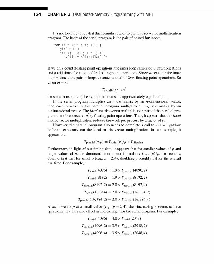
124 CHAPTER 3 Distributed-Memory Programming with MPI
It’s not too hard to see that this formula applies to our matrix-vector multiplicationprogram. The heart of the serial program is the pair of nested for loops:
for (i = 0; i < m; i++) {y[i] = 0.0;for (j = 0; j < n; j++)
y[i] += A[i∗n+j]∗x[j];}
If we only count floating point operations, the inner loop carries out n multiplicationsand n additions, for a total of 2n floating point operations. Since we execute the innerloop m times, the pair of loops executes a total of 2mn floating point operations. Sowhen m= n,
Tserial(n)≈ an2
for some constant a. (The symbol ≈ means “is approximately equal to.”)If the serial program multiplies an n× n matrix by an n-dimensional vector,
then each process in the parallel program multiplies an n/p× n matrix by ann-dimensional vector. The local matrix-vector multiplication part of the parallel pro-gram therefore executes n2/p floating point operations. Thus, it appears that this localmatrix-vector multiplication reduces the work per process by a factor of p.
However, the parallel program also needs to complete a call to MPI Allgatherbefore it can carry out the local matrix-vector multiplication. In our example, itappears that
Tparallel(n,p)= Tserial(n)/p+Tallgather.
Furthermore, in light of our timing data, it appears that for smaller values of p andlarger values of n, the dominant term in our formula is Tserial(n)/p. To see this,observe first that for small p (e.g., p= 2,4), doubling p roughly halves the overallrun-time. For example,
Tserial(4096)= 1.9×Tparallel(4096,2)
Tserial(8192)= 1.9×Tparallel(8192,2)
Tparallel(8192,2)= 2.0×Tparallel(8192,4)
Tserial(16,384)= 2.0×Tparallel(16,384,2)
Tparallel(16,384,2)= 2.0×Tparallel(16,384,4)
Also, if we fix p at a small value (e.g., p= 2,4), then increasing n seems to haveapproximately the same effect as increasing n for the serial program. For example,
Tserial(4096)= 4.0×Tserial(2048)
Tparallel(4096,2)= 3.9×Tparallel(2048,2)
Tparallel(4096,4)= 3.5×Tparallel(2048,4)

3.6 Performance Evaluation of MPI Programs 125
Tserial(8192)= 4.2×Tserial(4096)
Tparallel(8192,2)= 4.2×Tparallel(4096,2)
Tparallel(8192,4)= 3.9×Tparallel(8192,4)
These observations suggest that the parallel run-times are behaving much as the run-times of the serial program—that is, Tparallel(n,p) is approximately Tserial(n)/p—sothe overhead Tallgather has little effect on the performance.
On the other hand, for small n and large p these patterns break down. For example,
Tparallel(1024,8)= 1.0×Tparallel(1024,16)
Tparallel(2048,16)= 1.5×Tparallel(1024,16)
Thus, it appears that for small n and large p, the dominant term in our formula forTparallel is Tallgather.
3.6.3 Speedup and efficiencyRecall that the most widely used measure of the relation between the serial and theparallel run-times is the speedup. It’s just the ratio of the serial run-time to the parallelrun-time:
S(n,p)=Tserial(n)
Tparallel(n,p).
The ideal value for S(n,p) is p. If S(n,p)= p, then our parallel program withcomm sz= p processes is running p times faster than the serial program. In practice,this speedup, sometimes called linear speedup, is rarely achieved. Our matrix-vectormultiplication program got the speedups shown in Table 3.6. For small p and large n,our program obtained nearly linear speedup. On the other hand, for large p andsmall n, the speedup was considerably less than p. The worst case was n= 1024and p= 16, when we only managed a speedup of 2.4.
Table 3.6 Speedups of Parallel Matrix-VectorMultiplication
Order of Matrix
comm sz 1024 2048 4096 8192 16,384
1 1.0 1.0 1.0 1.0 1.02 1.8 1.9 1.9 1.9 2.04 2.1 3.1 3.6 3.9 3.98 2.4 4.8 6.5 7.5 7.916 2.4 6.2 10.8 14.2 15.5

126 CHAPTER 3 Distributed-Memory Programming with MPI
Table 3.7 Efficiencies of ParallelMatrix-Vector Multiplication
Order of Matrix
comm sz 1024 2048 4096 8192 16,384
1 1.00 1.00 1.00 1.00 1.002 0.89 0.94 0.97 0.96 0.984 0.51 0.78 0.89 0.96 0.988 0.30 0.61 0.82 0.94 0.9816 0.15 0.39 0.68 0.89 0.97
Also recall that another widely used measure of parallel performance is parallelefficiency. This is “per process” speedup:
E(n,p)=S(n,p)
p=
Tserial(n)
p×Tparallel(n,p).
Linear speedup corresponds to a parallel efficiency of p/p= 1.0, and, in general, weexpect that our efficiencies will be less than 1.
The efficiencies for the matrix-vector multiplication program are shown inTable 3.7. Once again, for small p and large n our parallel efficiencies are near linear,and for large p and small n, they are very far from linear.
3.6.4 ScalabilityOur parallel matrix-vector multiplication program doesn’t come close to obtaininglinear speedup for small n and large p. Does this mean that it’s not a good program?Many computer scientists answer this question by looking at the “scalability” of theprogram. Recall that very roughly speaking, a program is scalable if the problemsize can be increased at a rate so that the efficiency doesn’t decrease as the numberof processes increase.
The problem with this definition is the phrase “the problem size can be increasedat a rate . . . ” Consider two parallel programs: program A and program B. Suppose thatif p≥ 2, the efficiency of program A is 0.75, regardless of problem size. Also supposethat the efficiency of program B is n/(625p), provided p≥ 2 and 1000≤ n≤ 625p.Then according to our “definition,” both programs are scalable. For program A, therate of increase needed to maintain constant efficiency is 0, while for program B ifwe increase n at the same rate as we increase p, we’ll maintain a constant efficiency.For example, if n= 1000 and p= 2, the efficiency of B is 0.80. If we then double pto 4 and we leave the problem size at n= 1000, the efficiency will drop to 0.40, butif we also double the problem size to n= 2000, the efficiency will remain constantat 0.80. Program A is thus more scalable than B, but both satisfy our definition ofscalability.

3.7 A Parallel Sorting Algorithm 127
Looking at our table of parallel efficiencies (Table 3.7), we see that our matrix-vector multiplication program definitely doesn’t have the same scalability as programA: in almost every case when p is increased, the efficiency decreases. On the otherhand, the program is somewhat like program B: if p≥ 2 and we increase both pand n by a factor of 2, the parallel efficiency, for the most part, actually increases.Furthermore, the only exceptions occur when we increase p from 2 to 4, and whencomputer scientists discuss scalability, they’re usually interested in large values ofp. When p is increased from 4 to 8 or from 8 to 16, our efficiency always increaseswhen we increase n by a factor of 2.
Recall that programs that can maintain a constant efficiency without increas-ing the problem size are sometimes said to be strongly scalable. Programs thatcan maintain a constant efficiency if the problem size increases at the same rate asthe number of processes are sometimes said to be weakly scalable. Program A isstrongly scalable, and program B is weakly scalable. Furthermore, our matrix-vectormultiplication program is also apparently weakly scalable.
3.7 A PARALLEL SORTING ALGORITHMWhat do we mean by a parallel sorting algorithm in a distributed-memory envi-ronment? What would its “input” be and what would its “output” be? The answersdepend on where the keys are stored. We can start or finish with the keys distributedamong the processes or assigned to a single process. In this section we’ll look at analgorithm that starts and finishes with the keys distributed among the processes. InProgramming Assignment 3.8 we’ll look at an algorithm that finishes with the keysassigned to a single process.
If we have a total of n keys and p= comm sz processes, our algorithm will startand finish with n/p keys assigned to each process. (As usual, we’ll assume n is evenlydivisible by p.) At the start, there are no restrictions on which keys are assigned towhich processes. However, when the algorithm terminates,
. the keys assigned to each process should be sorted in (say) increasing order, and. if 0≤ q< r < p, then each key assigned to process q should be less than or equalto every key assigned to process r.
So if we lined up the keys according to process rank—keys from process 0 first, thenkeys from process 1, and so on—then the keys would be sorted in increasing order.For the sake of explicitness, we’ll assume our keys are ordinary ints.
3.7.1 Some simple serial sorting algorithmsBefore starting, let’s look at a couple of simple serial sorting algorithms. Perhaps thebest known serial sorting algorithm is bubble sort (see Program 3.14). The array astores the unsorted keys when the function is called, and the sorted keys when thefunction returns. The number of keys in a is n. The algorithm proceeds by comparing
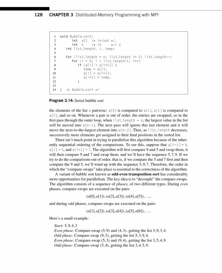
128 CHAPTER 3 Distributed-Memory Programming with MPI
1 void Bubble sort(2 int a[] /∗ in/out ∗/,3 int n /∗ in ∗/) {4 int list length, i, temp;56 for (list length = n; list length >= 2; list length−−)7 for (i = 0; i < list length−1; i++)8 if (a[i] > a[i+1]) {9 temp = a[i];
10 a[i] = a[i+1];11 a[i+1] = temp;12 }
1314 } /∗ Bubble sort ∗/
Program 3.14: Serial bubble sort
the elements of the list a pairwise: a[0] is compared to a[1], a[1] is compared toa[2], and so on. Whenever a pair is out of order, the entries are swapped, so in thefirst pass through the outer loop, when list length = n, the largest value in the listwill be moved into a[n−1]. The next pass will ignore this last element and it willmove the next-to-the-largest element into a[n−2]. Thus, as list length decreases,successively more elements get assigned to their final positions in the sorted list.
There isn’t much point in trying to parallelize this algorithm because of the inher-ently sequential ordering of the comparisons. To see this, suppose that a[i−1] = 9,a[i] = 5, and a[i+1] = 7. The algorithm will first compare 9 and 5 and swap them, itwill then compare 9 and 7 and swap them, and we’ll have the sequence 5,7,9. If wetry to do the comparisons out of order, that is, if we compare the 5 and 7 first and thencompare the 9 and 5, we’ll wind up with the sequence 5,9,7. Therefore, the order inwhich the “compare-swaps” take place is essential to the correctness of the algorithm.
A variant of bubble sort known as odd-even transposition sort has considerablymore opportunities for parallelism. The key idea is to “decouple” the compare-swaps.The algorithm consists of a sequence of phases, of two different types. During evenphases, compare-swaps are executed on the pairs
(a[0],a[1]),(a[2],a[3]),(a[4],a[5]), . . . ,
and during odd phases, compare-swaps are executed on the pairs
(a[1],a[2]),(a[3],a[4]),(a[5],a[6]), . . . .
Here’s a small example:
Start: 5,9,4,3Even phase: Compare-swap (5,9) and (4,3), getting the list 5,9,3,4.Odd phase: Compare-swap (9,3), getting the list 5,3,9,4.Even phase: Compare-swap (5,3) and (9,4), getting the list 3,5,4,9.Odd phase: Compare-swap (5,4), getting the list 3,4,5,9.

3.7 A Parallel Sorting Algorithm 129
This example required four phases to sort a four-element list. In general, it mayrequire fewer phases, but the following theorem guarantees that we can sort a listof n elements in at most n phases:
Theorem. Suppose A is a list with n keys, and A is the input to the odd-even transpositionsort algorithm. Then, after n phases A will be sorted.
Program 3.15 shows code for a serial odd-even transposition sort function.
1 void Odd even sort(2 int a[] /∗ in/out ∗/,3 int n /∗ in ∗/) {4 int phase, i, temp;56 for (phase = 0; phase < n; phase++)7 if (phase % 2 == 0) { /∗ Even phase ∗/8 for (i = 1; i < n; i += 2)9 if (a[i−1] > a[i]) {
10 temp = a[i];11 a[i] = a[i−1];12 a[i−1] = temp;13 }
14 } else { /∗ Odd phase ∗/15 for (i = 1; i < n−1; i += 2)16 if (a[i] > a[i+1]) {17 temp = a[i];18 a[i] = a[i+1];19 a[i+1] = temp;20 }
21 }
22 } /∗ Odd even sort ∗/
Program 3.15: Serial odd-even transposition sort
3.7.2 Parallel odd-even transposition sortIt should be clear that odd-even transposition sort has considerably more opportu-nities for parallelism than bubble sort, because all of the compare-swaps in a singlephase can happen simultaneously. Let’s try to exploit this.
There are a number of possible ways to apply Foster’s methodology. Here’s one:
. Tasks: Determine the value of a[i] at the end of phase j.. Communications: The task that’s determining the value of a[i] needs to commu-nicate with either the task determining the value of a[i−1] or a[i+1]. Also thevalue of a[i] at the end of phase j needs to be available for determining the valueof a[i] at the end of phase j+ 1.
This is illustrated in Figure 3.12, where we’ve labeled the tasks determining the valueof a[i] with a[i].

130 CHAPTER 3 Distributed-Memory Programming with MPI
a[i - 1]
a[i - 1] phase j + 1
phase ja[i]
a[i] a[i + 1]
a[i + 1]
FIGURE 3.12
Communications among tasks in an odd-even sort. Tasks determining a[i] are labeledwith a[i].
Now recall that when our sorting algorithm starts and finishes execution, eachprocess is assigned n/p keys. In this case our aggregation and mapping are at leastpartially specified by the description of the problem. Let’s look at two cases.
When n= p, Figure 3.12 makes it fairly clear how the algorithm should proceed.Depending on the phase, process i can send its current value, a[i], either to processi− 1 or process i+ 1. At the same time, it should receive the value stored on processi− 1 or process i+ 1, respectively, and then decide which of the two values it shouldstore as a[i] for the next phase.
However, it’s unlikely that we’ll actually want to apply the algorithm when n= p,since we’re unlikely to have more than a few hundred or a few thousand processorsat our disposal, and sorting a few thousand values is usually a fairly trivial mat-ter for a single processor. Furthermore, even if we do have access to thousands oreven millions of processors, the added cost of sending and receiving a message foreach compare-exchange will slow the program down so much that it will be useless.Remember that the cost of communication is usually much greater than the cost of“local” computation—for example, a compare-swap.
How should this be modified when each process is storing n/p> 1 elements?(Recall that we’re assuming that n is evenly divisible by p.) Let’s look at an example.Suppose we have p= 4 processes and n= 16 keys assigned, as shown in Table 3.8.In the first place, we can apply a fast serial sorting algorithm to the keys assignedto each process. For example, we can use the C library function qsort on each pro-cess to sort the local keys. Now if we had one element per process, 0 and 1 wouldexchange elements, and 2 and 3 would exchange. So let’s try this: Let’s have 0 and 1exchange all their elements and 2 and 3 exchange all of theirs. Then it would seemnatural for 0 to keep the four smaller elements and 1 to keep the larger. Similarly,2 should keep the smaller and 3 the larger. This gives us the situation shown in thethird row of the the table. Once again, looking at the one element per process case,in phase 1, processes 1 and 2 exchange their elements and processes 0 and 3 areidle. If process 1 keeps the smaller and 2 the larger elements, we get the distributionshown in the fourth row. Continuing this process for two more phases results in asorted list. That is, each process’ keys are stored in increasing order, and if q< r,

3.7 A Parallel Sorting Algorithm 131
Table 3.8 Parallel Odd-Even Transposition Sort
Process
Time 0 1 2 3
Start 15, 11, 9, 16 3, 14, 8, 7 4, 6, 12, 10 5, 2, 13, 1After Local Sort 9, 11, 15, 16 3, 7, 8, 14 4, 6, 10, 12 1, 2, 5, 13After Phase 0 3, 7, 8, 9 11, 14, 15, 16 1, 2, 4, 5 6, 10, 12, 13After Phase 1 3, 7, 8, 9 1, 2, 4, 5 11, 14, 15, 16 6, 10, 12, 13After Phase 2 1, 2, 3, 4 5, 7, 8, 9 6, 10, 11, 12 13, 14, 15, 16After Phase 3 1, 2, 3, 4 5, 6, 7, 8 9, 10, 11, 12 13, 14, 15, 16
then the keys assigned to process q are less than or equal to the keys assigned toprocess r.
In fact, our example illustrates the worst-case performance of this algorithm:
Theorem. If parallel odd-even transposition sort is run with p processes, then after pphases, the input list will be sorted.
The parallel algorithm is clear to a human computer:
Sort local keys;for (phase = 0; phase < comm sz; phase++) {
partner = Compute partner(phase, my rank);if (I’m not idle) {
Send my keys to partner;Receive keys from partner;if (my rank < partner)
Keep smaller keys;else
Keep larger keys;}
}
However, there are some details that we need to clear up before we can convert thealgorithm into an MPI program.
First, how do we compute the partner rank? And what is the partner rank whena process is idle? If the phase is even, then odd-ranked partners exchange withmy rank−1 and even-ranked partners exchange with my rank+1. In odd phases, thecalculations are reversed. However, these calculations can return some invalid ranks:if my rank = 0 or my rank = comm sz−1, the partner rank can be −1 or comm sz.But when either partner = −1 or partner = comm sz, the process should be idle.We can use the rank computed by Compute partner to determine whether a processis idle:
if (phase % 2 == 0) /∗ Even phase ∗/if (my rank % 2 != 0) /∗ Odd rank ∗/
partner = my rank − 1;else /∗ Even rank ∗/
partner = my rank + 1;

132 CHAPTER 3 Distributed-Memory Programming with MPI
else /∗ Odd phase ∗/if (my rank % 2 != 0) /∗ Odd rank ∗/
partner = my rank + 1;else /∗ Even rank ∗/
partner = my rank − 1;if (partner == −1 | | partner == comm sz)
partner = MPI PROC NULL;
MPI PROC NULL is a constant defined by MPI. When it’s used as the source or destina-tion rank in a point-to-point communication, no communication will take place andthe call to the communication will simply return.
3.7.3 Safety in MPI programsIf a process is not idle, we might try to implement the communication with a call toMPI Send and a call to MPI Recv:
MPI Send(my keys, n/comm sz, MPI INT, partner, 0, comm);MPI Recv(temp keys, n/comm sz, MPI INT, partner, 0, comm,
MPI STATUS IGNORE);
This, however, might result in the programs’ hanging or crashing. Recall that the MPIstandard allows MPI Send to behave in two different ways: it can simply copy themessage into an MPI-managed buffer and return, or it can block until the matchingcall to MPI Recv starts. Furthermore, many implementations of MPI set a thresholdat which the system switches from buffering to blocking. That is, messages that arerelatively small will be buffered by MPI Send, but for larger messages, it will block.If the MPI Send executed by each process blocks, no process will be able to startexecuting a call to MPI Recv, and the program will hang or deadlock, that is, eachprocess is blocked waiting for an event that will never happen.
A program that relies on MPI-provided buffering is said to be unsafe. Such aprogram may run without problems for various sets of input, but it may hang orcrash with other sets. If we use MPI Send and MPI Recv in this way, our programwill be unsafe, and it’s likely that for small values of n the program will run withoutproblems, while for larger values of n, it’s likely that it will hang or crash.
There are a couple of questions that arise here:
1. In general, how can we tell if a program is safe?2. How can we modify the communication in the parallel odd-even sort program so
that it is safe?
To answer the first question, we can use an alternative to MPI Send defined by the MPIstandard. It’s called MPI Ssend. The extra “s” stands for synchronous and MPI Ssendis guaranteed to block until the matching receive starts. So, we can check whethera program is safe by replacing the calls to MPI Send with calls to MPI Ssend. If theprogram doesn’t hang or crash when it’s run with appropriate input and comm sz,then the original program was safe. The arguments to MPI Ssend are the same as thearguments to MPI Send:

3.7 A Parallel Sorting Algorithm 133
int MPI Ssend(void∗ msg buf p /∗ in ∗/,int msg size /∗ in ∗/,MPI Datatype msg type /∗ in ∗/,int dest /∗ in ∗/,int tag /∗ in ∗/,MPI Comm communicator /∗ in ∗/);
The answer to the second question is that the communication must be restructured.The most common cause of an unsafe program is multiple processes simultaneouslyfirst sending to each other and then receiving. Our exchanges with partners is oneexample. Another example is a “ring pass,” in which each process q sends to theprocess with rank q+ 1, except that process comm sz− 1 sends to 0:
MPI Send(msg, size, MPI INT, (my rank+1) % comm sz, 0, comm);MPI Recv(new msg, size, MPI INT, (my rank+comm sz−1) % comm sz,
0, comm, MPI STATUS IGNORE).
In both settings, we need to restructure the communications so that some of the pro-cesses receive before sending. For example, the preceding communications could berestructured as follows:
if (my rank % 2 == 0) {MPI Send(msg, size, MPI INT, (my rank+1) % comm sz, 0, comm);MPI Recv(new msg, size, MPI INT, (my rank+comm sz−1) % comm sz,
0, comm, MPI STATUS IGNORE).} else {
MPI Recv(new msg, size, MPI INT, (my rank+comm sz−1) % comm sz,0, comm, MPI STATUS IGNORE).
MPI Send(msg, size, MPI INT, (my rank+1) % comm sz, 0, comm);}
It’s fairly clear that this will work if comm sz is even. If, say, comm sz= 4, thenprocesses 0 and 2 will first send to 1 and 3, respectively, while processes 1 and 3 willreceive from 0 and 2, respectively. The roles are reversed for the next send-receivepairs: processes 1 and 3 will send to 2 and 0, respectively, while 2 and 0 will receivefrom 1 and 3.
However, it may not be clear that this scheme is also safe if comm sz is odd (andgreater than 1). Suppose, for example, that comm sz= 5. Then, Figure 3.13 shows apossible sequence of events. The solid arrows show a completed communication, andthe dashed arrows show a communication waiting to complete.
MPI provides an alternative to scheduling the communications ourselves—wecan call the function MPI Sendrecv:
int MPI Sendrecv(void∗ send buf p /∗ in ∗/,int send buf size /∗ in ∗/,MPI Datatype send buf type /∗ in ∗/,int dest /∗ in ∗/,int send tag /∗ in ∗/,

134 CHAPTER 3 Distributed-Memory Programming with MPI
0
4 3
Time 0 Time 1
Time 2
1
2
0
4 3
1
2
0
4 3
1
2
FIGURE 3.13
Safe communication with five processes
void∗ recv buf p /∗ out ∗/,int recv buf size /∗ in ∗/,MPI Datatype recv buf type /∗ in ∗/,int source /∗ in ∗/,int recv tag /∗ in ∗/,MPI Comm communicator /∗ in ∗/,MPI Status∗ status p /∗ in ∗/);
This function carries out a blocking send and a receive in a single call. The destand the source can be the same or different. What makes it especially useful is thatthe MPI implementation schedules the communications so that the program won’thang or crash. The complex code we used earlier—the code that checks whether theprocess rank is odd or even—can be replaced with a single call to MPI Sendrecv. Ifit happens that the send and the receive buffers should be the same, MPI provides thealternative:
int MPI Sendrecv replace(void∗ buf p /∗ in/out ∗/,int buf size /∗ in ∗/,MPI Datatype buf type /∗ in ∗/,int dest /∗ in ∗/,int send tag /∗ in ∗/,int source /∗ in ∗/,int recv tag /∗ in ∗/,MPI Comm communicator /∗ in ∗/,MPI Status∗ status p /∗ in ∗/);
3.7.4 Final details of parallel odd-even sortRecall that we had developed the following parallel odd-even transposition sortalgorithm:

3.7 A Parallel Sorting Algorithm 135
Sort local keys;for (phase = 0; phase < comm sz; phase++) {
partner = Compute partner(phase, my rank);if (I’m not idle) {
Send my keys to partner;Receive keys from partner;if (my rank < partner)
Keep smaller keys;else
Keep larger keys;}
}
In light of our discussion of safety in MPI, it probably makes sense to implement thesend and the receive with a single call to MPI Sendrecv:
MPI Sendrecv(my keys, n/comm sz, MPI INT, partner, 0,recv keys, n/comm sz, MPI INT, partner, 0, comm,MPI Status ignore);
It only remains to identify which keys we keep. Suppose for the moment thatwe want to keep the smaller keys. Then we want to keep the smallest n/p keys in acollection of 2n/p keys. An obvious approach to doing this is to sort (using a serialsorting algorithm) the list of 2n/p keys and keep the first half of the list. However,sorting is a relatively expensive operation, and we can exploit the fact that we alreadyhave two sorted lists of n/p keys to reduce the cost by merging the two lists into asingle list. In fact, we can do even better, because we don’t need a fully generalmerge: once we’ve found the smallest n/p keys, we can quit. See Program 3.16.
To get the largest n/p keys, we simply reverse the order of the merge, that is, startwith local n−1 and work backwards through the arrays. A final improvement avoidscopying the arrays and simply swaps pointers (see Exercise 3.28).
Run-times for the version of parallel odd-even sort with the “final improvement”are shown in Table 3.9. Note that if parallel odd-even sort is run on a single processor,it will use whatever serial sorting algorithm we use to sort the local keys, so the timesfor a single process use serial quicksort, not serial odd-even sort, which would bemuch slower. We’ll take a closer look at these times in Exercise 3.27.
Table 3.9 Run-Times of Parallel Odd-EvenSort (times are in milliseconds)
Number of Keys (in thousands)
Processes 200 400 800 1600 3200
1 88 190 390 830 18002 43 91 190 410 8604 22 46 96 200 4308 12 24 51 110 22016 7.5 14 29 60 130

136 CHAPTER 3 Distributed-Memory Programming with MPI
void Merge low(int my keys[], /∗ in/out ∗/int recv keys[], /∗ in ∗/int temp keys[], /∗ scratch ∗/int local n /∗ = n/p, in ∗/) {
int m i, r i, t i;
m i = r i = t i = 0;while (t i < local n) {
if (my keys[m i] <= recv keys[r i]) {temp keys[t i] = my keys[m i];t i++; m i++;
} else {temp keys[t i] = recv keys[r i];t i++; r i++;
}
}
for (m i = 0; m i < local n; m i++)my keys[m i] = temp keys[m i];
} /∗ Merge low ∗/
Program 3.16: The Merge low function in parallel odd-even transposition sort
3.8 SUMMARYMPI, or the Message-Passing Interface, is a library of functions that can be calledfrom C, C++, or Fortran programs. Many systems use mpicc to compile MPI pro-grams and mpiexec to run them. C MPI programs should include the mpi.h headerfile to get function prototypes and macros defined by MPI.
MPI Init does the setup needed to run MPI. It should be called before other MPIfunctions are called. When your program doesn’t use argc and argv, NULL can bepassed for both arguments.
In MPI a communicator is a collection of processes that can send messages toeach other. After an MPI program is started, MPI always creates a communicatorconsisting of all the processes. It’s called MPI COMM WORLD.
Many parallel programs use the single program, multiple data, or SPMD,approach, whereby running a single program obtains the effect of running multipledifferent programs by including branches on data such as the process rank. Whenyou’re done using MPI, you should call MPI Finalize.
To send a message from one MPI process to another, you can use MPI Send. Toreceive a message, you can use MPI Recv. The arguments to MPI Send describe thecontents of the message and its destination. The arguments to MPI Recv describethe storage that the message can be received into, and where the message should bereceived from. MPI Recv is blocking, that is, a call to MPI Recv won’t return until the

3.8 Summary 137
message has been received (or an error has occurred). The behavior of MPI Send isdefined by the MPI implementation. It can either block, or it can buffer the message.When it blocks, it won’t return until the matching receive has started. If the messageis buffered, MPI will copy the message into its own private storage, and MPI Sendwill return as soon as the message is copied.
When you’re writing MPI programs, it’s important to differentiate between localand global variables. Local variables have values that are specific to the process onwhich they’re defined, while global variables are the same on all the processes. Inthe trapezoidal rule program, the total number of trapezoids n was a global variable,while the left and right endpoints of each process’ interval were local variables.
Most serial programs are deterministic, meaning if we run the same program withthe same input we’ll get the same output. Recall that parallel programs often don’tpossess this property—if multiple processes are operating more or less independently,the processes may reach various points at different times, depending on events outsidethe control of the process. Thus, parallel programs can be nondeterministic, thatis, the same input can result in different outputs. If all the processes in an MPI programare printing output, the order in which the output appears may be different each timethe program is run. For this reason, it’s common in MPI programs to have a singleprocess (e.g., process 0) handle all the output. This rule of thumb is usually ignoredduring debugging, when we allow each process to print debug information.
Most MPI implementations allow all the processes to print to stdout and stderr.However, every implementation we’ve encountered only allows at most one process(usually process 0 in MPI COMM WORLD) to read from stdin.
Collective communications involve all the processes in a communicator, sothey’re different from MPI Send and MPI Recv, which only involve two processes.To distinguish between the two types of communications, functions such as MPI Sendand MPI Recv are often called point-to-point communications.
Two of the most commonly used collective communication functions areMPI Reduce and MPI Allreduce. MPI Reduce stores the result of a global opera-tion (e.g., a global sum) on a single designated process, while MPI Allreduce storesthe result on all the processes in the communicator.
In MPI functions such as MPI Reduce, it may be tempting to pass the same actualargument to both the input and output buffers. This is called argument aliasing, andMPI explicitly prohibits aliasing an output argument with another argument.
We learned about a number of other important MPI collective communications:
. MPI Bcast sends data from a single process to all the processes in a communicator.This is very useful if, for example, process 0 reads data from stdin and the dataneeds to be sent to all the processes.. MPI Scatter distributes the elements of an array among the processes. If the arrayto be distributed contains n elements, and there are p processes, then the first n/pare sent to process 0, the next n/p to process 1, and so on.. MPI Gather is the “inverse operation” to MPI Scatter. If each process stores asubarray containing m elements, MPI Gather will collect all of the elements onto

138 CHAPTER 3 Distributed-Memory Programming with MPI
a designated process, putting the elements from process 0 first, then the elementsfrom process 1, and so on.. MPI Allgather is like MPI Gather except that it collects all of the elements ontoall the processes.. MPI Barrier approximately synchronizes the processes; no process can returnfrom a call to MPI Barrier until all the processes in the communicator havestarted the call.
In distributed-memory systems there is no globally shared-memory, so partition-ing global data structures among the processes is a key issue in writing MPI programs.For ordinary vectors and arrays, we saw that we could use block partitioning, cyclicpartitioning, or block-cyclic partitioning. If the global vector or array has n compo-nents and there are p processes, a block partition assigns the first n/p to process 0,the next n/p to process 1, and so on. A cyclic partition assigns the elements in a“round-robin” fashion: the first element goes to 0, the next to 1, . . . , the pth to p− 1.After assigning the first p elements, we return to process 0, so the (p+ 1)st goes toprocess 0, the (p+ 2)nd to process 1, and so on. A block-cyclic partition assignsblocks of elements to the processes in a cyclic fashion.
Compared to operations involving only the CPU and main memory, sending mes-sages is expensive. Furthermore, sending a given volume of data in fewer messagesis usually less expensive than sending the same volume in more messages. Thus, itoften makes sense to reduce the number of messages sent by combining the con-tents of multiple messages into a single message. MPI provides three methods fordoing this: the count argument to communication functions, derived datatypes, andMPI Pack/Unpack. Derived datatypes describe arbitrary collections of data by spec-ifying the types of the data items and their relative positions in memory. In thischapter we took a brief look at the use of MPI Type create struct to build a deriveddatatype. In the exercises, we’ll explore some other methods, and we’ll take a look atMPI Pack/Unpack
When we time parallel programs, we’re usually interested in elapsed time or “wallclock time,” which is the total time taken by a block of code. It includes time in usercode, time in library functions, time in operating system functions started by theuser code, and idle time. We learned about two methods for finding wall clock time:GET TIME and MPI Wtime. GET TIME is a macro defined in the file timer.h that canbe downloaded from the book’s website. It can be used in serial code as follows:
#include "timer.h" // From the book’s website. . .double start, finish, elapsed;. . .GET TIME(start);/∗ Code to be timed ∗/. . .GET TIME(finish);elapsed = finish − start;printf("Elapsed time = %e seconds\n", elapsed);

3.8 Summary 139
MPI provides a function, MPI Wtime, that can be used instead of GET TIME. In spiteof this, timing parallel code is more complex, since ideally we’d like to synchronizethe processes at the start of the code, and then report the time it took for the “slowest”process to complete the code. MPI Barrier does a fairly good job of synchronizingthe processes. A process that calls it will block until all the processes in the commu-nicator have called it. We can use the following template for finding the run-time ofMPI code:
double start, finish, loc elapsed, elapsed;. . .MPI Barrier(comm);start = MPI Wtime();/∗ Code to be timed ∗/. . .finish = MPI Wtime();loc elapsed = finish − start;MPI Reduce(&loc elapsed, &elapsed, 1, MPI DOUBLE, MPI MAX,
0, comm);if (my rank == 0)
printf("Elapsed time = %e seconds\n", elapsed);
A further problem with taking timings lies in the fact that there is ordinarilyconsiderable variation if the same code is timed repeatedly. For example, the oper-ating system may idle one or more of our processes so that other processes can run.Therefore, we typically take several timings and report their minimum.
After taking timings, we can use the speedup or the efficiency to evaluate theprogram performance. The speedup is the ratio of the serial run-time to the parallelrun-time, and the efficiency is the speedup divided by the number of parallel pro-cesses. The ideal value for speedup is p, the number of processes, and the ideal valuefor the efficiency is 1. We rarely achieve these ideals, but it’s not uncommon to seeprograms that get close to these values, especially when p is small and n, the prob-lem size, is large. Parallel overhead is the part of the parallel run-time that’s dueto any additional work that isn’t done by the serial program. In MPI programs, par-allel overhead will come from communication. When p is large and n is small, it’snot unusual for parallel overhead to dominate the total run-time and speedups andefficiencies can be quite low. If it’s possible to increase the problem size (n) so thatthe efficiency doesn’t decrease as p is increased, a parallel program is said to bescalable.
Recall that MPI Send can either block or buffer its input. An MPI program isunsafe if its correct behavior depends on the fact that MPI Send is buffering its input.This typically happens when multiple processes first call MPI Send and then callMPI Recv. If the calls to MPI Send don’t buffer the messages, then they’ll block untilthe matching calls to MPI Recv have started. However, this will never happen. Forexample, if both process 0 and process 1 want to send data to each other, and bothsend first and then receive, process 0 will wait forever for process 1 to call MPI Recv,since process 1 is blocked in MPI Send, and process 1 will wait forever for process 0.

140 CHAPTER 3 Distributed-Memory Programming with MPI
That is, the processes will hang or deadlock—they’ll block forever waiting for eventsthat will never happen.
An MPI program can be checked for safety by replacing each call to MPI Sendwith a call to MPI Ssend. MPI Ssend takes the same arguments as MPI Send, but italways blocks until the matching receive has started. The extra “s” stands for syn-chronous. If the program completes correctly with MPI Ssend for the desired inputsand communicator sizes, then the program is safe.
An unsafe MPI program can be made safe in several ways. The programmer canschedule the calls to MPI Send and MPI Recv so that some processes (e.g., even-ranked processes) first call MPI Send while others (e.g., odd-ranked processes) firstcall MPI Recv. Alternatively, we can use MPI Sendrecv or MPI Sendrecv replace.These functions execute both a send and a receive, but they’re guaranteed to schedulethem so that the program won’t hang or crash. MPI Sendrecv uses different argu-ments for the send and the receive buffers, while MPI Sendrecv replace uses thesame buffer for both.
3.9 EXERCISES
3.1. What happens in the greetings program if, instead of strlen(greeting) + 1,we use strlen(greeting) for the length of the message being sent by pro-cesses 1,2, . . . , comm sz−1? What happens if we use MAX STRING instead ofstrlen(greeting) + 1? Can you explain these results?
3.2. Modify the trapezoidal rule so that it will correctly estimate the integral evenif comm sz doesn’t evenly divide n. (You can still assume that n≥ comm sz.)
3.3. Determine which of the variables in the trapezoidal rule program are local andwhich are global.
3.4. Modify the program that just prints a line of output from each process(mpi output.c) so that the output is printed in process rank order: process0s output first, then process 1s, and so on.
3.5. In a binary tree, there is a unique shortest path from each node to the root. Thelength of this path is often called the depth of the node. A binary tree in whichevery nonleaf has two children is called a full binary tree, and a full binary treein which every leaf has the same depth is sometimes called a complete binarytree. See Figure 3.14. Use the principle of mathematical induction to provethat if T is a complete binary tree with n leaves, then the depth of the leavesis log2(n).
3.6. Suppose comm sz= 4 and suppose that x is a vector with n= 14 components.a. How would the components of x be distributed among the processes in a
program that used a block distribution?

3.9 Exercises 141
FIGURE 3.14
A complete binary tree
b. How would the components of x be distributed among the processes in aprogram that used a cyclic distribution?
c. How would the components of x be distributed among the processes in aprogram that used a block-cyclic distribution with blocksize b= 2?
You should try to make your distributions general so that they could be usedregardless of what comm sz and n are. You should also try to make your distri-butions “fair” so that if q and r are any two processes, the difference betweenthe number of components assigned to q and the number of componentsassigned to r is as small as possible.
3.7. What do the various MPI collective functions do if the communicator containsa single process?
3.8. Suppose comm sz= 8 and n= 16.a. Draw a diagram that shows how MPI Scatter can be implemented using
tree-structured communication with comm sz processes when process 0needs to distribute an array containing n elements.
b. Draw a diagram that shows how MPI Gather can be implemented usingtree-structured communication when an n-element array that has beendistributed among comm sz processes needs to be gathered onto process 0.
3.9. Write an MPI program that implements multiplication of a vector by a scalarand dot product. The user should enter two vectors and a scalar, all of whichare read in by process 0 and distributed among the processes. The results arecalculated and collected onto process 0, which prints them. You can assumethat n, the order of the vectors, is evenly divisible by comm sz.
3.10. In the Read vector function shown in Program 3.9, we use local n asthe actual argument for two of the formal arguments to MPI Scatter:send count and recv count. Why is it OK to alias these arguments?
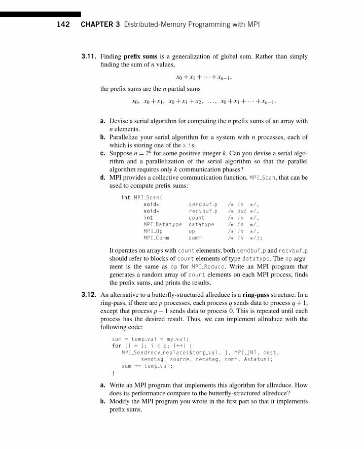
142 CHAPTER 3 Distributed-Memory Programming with MPI
3.11. Finding prefix sums is a generalization of global sum. Rather than simplyfinding the sum of n values,
x0+ x1+ ·· ·+ xn−1,
the prefix sums are the n partial sums
x0, x0+ x1, x0+ x1+ x2, . . . , x0+ x1+ ·· ·+ xn−1.
a. Devise a serial algorithm for computing the n prefix sums of an array withn elements.
b. Parallelize your serial algorithm for a system with n processes, each ofwhich is storing one of the x is.
c. Suppose n= 2k for some positive integer k. Can you devise a serial algo-rithm and a parallelization of the serial algorithm so that the parallelalgorithm requires only k communication phases?
d. MPI provides a collective communication function, MPI Scan, that can beused to compute prefix sums:
int MPI Scan(void∗ sendbuf p /∗ in ∗/,void∗ recvbuf p /∗ out ∗/,int count /∗ in ∗/,MPI Datatype datatype /∗ in ∗/,MPI Op op /∗ in ∗/,MPI Comm comm /∗ in ∗/);
It operates on arrays with count elements; both sendbuf p and recvbuf pshould refer to blocks of count elements of type datatype. The op argu-ment is the same as op for MPI Reduce. Write an MPI program thatgenerates a random array of count elements on each MPI process, findsthe prefix sums, and prints the results.
3.12. An alternative to a butterfly-structured allreduce is a ring-pass structure. In aring-pass, if there are p processes, each process q sends data to process q+ 1,except that process p− 1 sends data to process 0. This is repeated until eachprocess has the desired result. Thus, we can implement allreduce with thefollowing code:
sum = temp val = my val;for (i = 1; i < p; i++) {
MPI Sendrecv replace(&temp val, 1, MPI INT, dest,sendtag, source, recvtag, comm, &status);
sum += temp val;}
a. Write an MPI program that implements this algorithm for allreduce. Howdoes its performance compare to the butterfly-structured allreduce?
b. Modify the MPI program you wrote in the first part so that it implementsprefix sums.

3.9 Exercises 143
3.13. MPI Scatter and MPI Gather have the limitation that each process must sendor receive the same number of data items. When this is not the case, wemust use the MPI functions MPI Gatherv and MPI Scatterv. Look at theman pages for these functions, and modify your vector sum, dot product pro-gram so that it can correctly handle the case when n isn’t evenly divisible bycomm sz.
3.14. a. Write a serial C program that defines a two-dimensional array in the mainfunction. Just use numeric constants for the dimensions:
int two d[3][4];
Initialize the array in the main function. After the array is initialized, calla function that attempts to print the array. The prototype for the functionshould look something like this.
void Print two d(int two d[][], int rows, int cols);
After writing the function try to compile the program. Can you explainwhy it won’t compile?
b. After consulting a C reference (e.g., Kernighan and Ritchie [29]), modifythe program so that it will compile and run, but so that it still uses a two-dimensional C array.
3.15. What is the relationship between the “row-major” storage for two-dimensional arrays that we discussed in Section 2.2.3 and the one-dimensionalstorage we use in Section 3.4.9?
3.16. Suppose comm sz= 8 and the vector x= (0,1,2, . . . ,15) has been distributedamong the processes using a block distribution. Draw a diagram illustratingthe steps in a butterfly implementation of allgather of x.
3.17. MPI Type contiguous can be used to build a derived datatype from acollection of contiguous elements in an array. Its syntax is
int MPI Type contiguous(int count /∗ in ∗/,MPI Datatype old mpi t /∗ in ∗/,MPI Datatype∗ new mpi t p /∗ out ∗);
Modify the Read vector and Print vector functions so that they usean MPI datatype created by a call to MPI Type contiguous and a countargument of 1 in the calls to MPI Scatter and MPI Gather.
3.18. MPI Type vector can be used to build a derived datatype from a collectionof blocks of elements in an array as long as the blocks all have the same sizeand they’re equally spaced. Its syntax is
int MPI Type vector(int count /∗ in ∗/,int blocklength /∗ in ∗/,

144 CHAPTER 3 Distributed-Memory Programming with MPI
int stride /∗ in ∗/,MPI Datatype old mpi t /∗ in ∗/,MPI Datatype∗ new mpi t p /∗ out ∗/);
For example, if we had an array x of 18 doubles and we wanted to build atype corresponding to the elements in positions 0, 1, 6, 7, 12, 13, we couldcall
int MPI Type vector(3, 2, 6, MPI DOUBLE, &vect mpi t);
since the type consists of 3 blocks, each of which has 2 elements, and thespacing between the starts of the blocks is 6 doubles.
Write Read vector and Print vector functions that will allow process0 to read and print, respectively, a vector with a block-cyclic distribution. Butbeware! Do not use MPI Scatter or MPI Gather. There is a technical issueinvolved in using these functions with types created with MPI Type vector.(See, for example, [23].) Just use a loop of sends on process 0 in Read vectorand a loop of receives on process 0 in Print vector. The other processesshould be able to complete their calls to Read vector and Print vectorwith a single call to MPI Recv and MPI Send. The communication on process0 should use a derived datatype created by MPI Type vector. The calls onthe other processes should just use the count argument to the communica-tion function, since they’re receiving/sending elements that they will store incontiguous array locations.
3.19. MPI Type indexed can be used to build a derived datatype from arbitraryarray elements. Its syntax is
int MPI Type indexed(int count /∗ in ∗/,int array of blocklengths[] /∗ in ∗/,int array of displacements[] /∗ in ∗/,MPI Datatype old mpi t /∗ in ∗/,MPI Datatype∗ new mpi t p) /∗ out ∗/);
Unlike MPI Type create struct, the displacements are measured in units ofold mpi t—not bytes. Use MPI Type indexed to create a derived datatypethat corresponds to the upper triangular part of a square matrix. For example,in the 4× 4 matrix
0 1 2 34 5 6 78 9 10 11
12 13 14 15
the upper triangular part is the elements 0,1,2,3,5,6,7,10,11,15. Process0 should read in an n× n matrix as a one-dimensional array, create thederived datatype, and send the upper triangular part with a single call toMPI Send. Process 1 should receive the upper triangular part with a singlecall to MPI Recv and then print the data it received.

3.9 Exercises 145
3.20. The functions MPI Pack and MPI Unpack provide an alternative to deriveddatatypes for grouping data. MPI Pack copies the data to be sent, one block ata time, into a user-provided buffer. The buffer can then be sent and received.After the data is received, MPI Unpack can be used to unpack it from thereceive buffer. The syntax of MPI Pack is
int MPI Pack(void∗ in buf /∗ in ∗/,int in buf count /∗ in ∗/,MPI Datatype datatype /∗ in ∗/,void∗ pack buf /∗ out ∗/,int pack buf sz /∗ in ∗/,int∗ position p /∗ in/out ∗/,MPI Comm comm /∗ in ∗/);
We could therefore pack the input data to the trapezoidal rule program withthe following code:
char pack buf[100];int position = 0;
MPI Pack(&a, 1, MPI DOUBLE, pack buf, 100, &position, comm);MPI Pack(&b, 1, MPI DOUBLE, pack buf, 100, &position, comm);MPI Pack(&n, 1, MPI INT, pack buf, 100, &position, comm);
The key is the position argument. When MPI Pack is called, position shouldrefer to the first available slot in pack buf. When MPI Pack returns, it refersto the first available slot after the data that was just packed, so after process 0executes this code, all the processes can call MPI Bcast:
MPI Bcast(pack buf, 100, MPI PACKED, 0, comm);
Note that the MPI datatype for a packed buffer is MPI PACKED. Now the otherprocesses can unpack the data using: MPI Unpack:
int MPI Unpack(void∗ pack buf /∗ in ∗/,int pack buf sz /∗ in ∗/,int∗ position p /∗ in/out ∗/,void∗ out buf /∗ out ∗/,int out buf count /∗ in ∗/,MPI Datatype datatype /∗ in ∗/,MPI Comm comm /∗ in ∗/);
This can be used by “reversing” the steps in MPI Pack, that is, the data isunpacked one block at a time starting with position = 0.
Write another Get input function for the trapezoidal rule program. Thisone should use MPI Pack on process 0 and MPI Unpack on the other processes.
3.21. How does your system compare to ours? What run-times does your systemget for matrix-vector multiplication? What kind of variability do you see in
146 CHAPTER 3 Distributed-Memory Programming with MPI
the times for a given value of comm sz and n? Do the results tend to clusteraround the minimum, the mean, or the median?
3.22. Time our implementation of the trapezoidal rule that uses MPI Reduce. Howwill you choose n, the number of trapezoids? How do the minimum timescompare to the mean and median times? What are the speedups? What are theefficiencies? On the basis of the data you collected, would you say that thetrapezoidal rule is scalable?
3.23. Although we don’t know the internals of the implementation of MPI Reduce,we might guess that it uses a structure similar to the binary tree we discussed.If this is the case, we would expect that its run-time would grow roughly atthe rate of log2(p), since there are roughly log2(p) levels in the tree. (Here,p= comm sz.) Since the run-time of the serial trapezoidal rule is roughly pro-portional to n, the number of trapezoids, and the parallel trapezoidal rulesimply applies the serial rule to n/p trapezoids on each process, with ourassumption about MPI Reduce, we get a formula for the overall run-time ofthe parallel trapezoidal rule that looks like
Tparallel(n,p)≈ a×n
p+ b log2(p)
for some constants a and b.a. Use the formula, the times you’ve taken in Exercise 3.22, and your favorite
program for doing mathematical calculations (e.g., MATLABR©
) to get aleast-squares estimate of the values of a and b.
b. Comment on the quality of the predicted run-times using the formula andthe values for a and b computed in part (a).
3.24. Take a look at Programming Assignment 3.7. The code that we outlined fortiming the cost of sending messages should work even if the count argumentis zero. What happens on your system when the count argument is 0? Canyou explain why you get a nonzero elapsed time when you send a zero-bytemessage?
3.25. If comm sz= p, we mentioned that the “ideal” speedup is p. Is it possible todo better?a. Consider a parallel program that computes a vector sum. If we only time
the vector sum—that is, we ignore input and output of the vectors—howmight this program achieve speedup greater than p?
b. A program that achieves speedup greater than p is said to have super-linear speedup. Our vector sum example only achieved superlinearspeedup by overcoming certain “resource limitations.” What were theseresource limitations? Is it possible for a program to obtain superlinearspeedup without overcoming resource limitations?
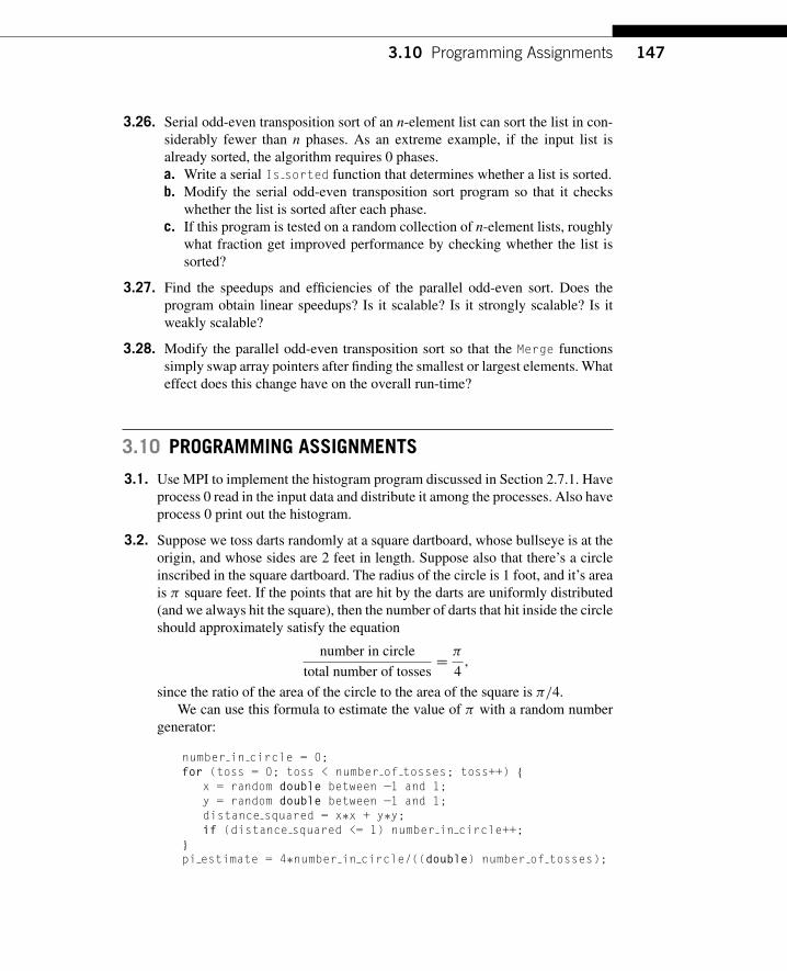
3.10 Programming Assignments 147
3.26. Serial odd-even transposition sort of an n-element list can sort the list in con-siderably fewer than n phases. As an extreme example, if the input list isalready sorted, the algorithm requires 0 phases.a. Write a serial Is sorted function that determines whether a list is sorted.b. Modify the serial odd-even transposition sort program so that it checks
whether the list is sorted after each phase.c. If this program is tested on a random collection of n-element lists, roughly
what fraction get improved performance by checking whether the list issorted?
3.27. Find the speedups and efficiencies of the parallel odd-even sort. Does theprogram obtain linear speedups? Is it scalable? Is it strongly scalable? Is itweakly scalable?
3.28. Modify the parallel odd-even transposition sort so that the Merge functionssimply swap array pointers after finding the smallest or largest elements. Whateffect does this change have on the overall run-time?
3.10 PROGRAMMING ASSIGNMENTS
3.1. Use MPI to implement the histogram program discussed in Section 2.7.1. Haveprocess 0 read in the input data and distribute it among the processes. Also haveprocess 0 print out the histogram.
3.2. Suppose we toss darts randomly at a square dartboard, whose bullseye is at theorigin, and whose sides are 2 feet in length. Suppose also that there’s a circleinscribed in the square dartboard. The radius of the circle is 1 foot, and it’s areais π square feet. If the points that are hit by the darts are uniformly distributed(and we always hit the square), then the number of darts that hit inside the circleshould approximately satisfy the equation
number in circle
total number of tosses=π
4,
since the ratio of the area of the circle to the area of the square is π/4.We can use this formula to estimate the value of π with a random number
generator:
number in circle = 0;for (toss = 0; toss < number of tosses; toss++) {
x = random double between −1 and 1;y = random double between −1 and 1;distance squared = x∗x + y∗y;if (distance squared <= 1) number in circle++;
}
pi estimate = 4∗number in circle/((double) number of tosses);

148 CHAPTER 3 Distributed-Memory Programming with MPI
This is called a “Monte Carlo” method, since it uses randomness (the darttosses).
Write an MPI program that uses a Monte Carlo method to estimate π .Process 0 should read in the total number of tosses and broadcast it to theother processes. Use MPI Reduce to find the global sum of the local variablenumber in circle, and have process 0 print the result. You may want to uselong long ints for the number of hits in the circle and the number of tosses,since both may have to be very large to get a reasonable estimate of π .
3.3. Write an MPI program that computes a tree-structured global sum. First writeyour program for the special case in which comm sz is a power of two. Then,after you’ve gotten this version working, modify your program so that it canhandle any comm sz.
3.4. Write an MPI program that computes a global sum using a butterfly. First writeyour program for the special case in which comm sz is a power of two. Can youmodify your program so that it will handle any number of processes?
3.5. Implement matrix-vector multiplication using a block-column distribution ofthe matrix. You can have process 0 read in the matrix and simply use a loopof sends to distribute it among the processes. Assume the matrix is square oforder n and that n is evenly divisible by comm sz. You may want to look at theMPI function MPI Reduce scatter.
3.6. Implement matrix-vector multiplication using a block-submatrix distributionof the matrix. Assume that the vectors are distributed among the diagonal pro-cesses. Once again, you can have process 0 read in the matrix and aggregatethe sub-matrices before sending them to the processes. Assume comm sz is aperfect square and that
√comm sz evenly divides the order of the matrix.
3.7. A ping-pong is a communication in which two messages are sent, first fromprocess A to process B (ping) and then from process B back to process A(pong). Timing blocks of repeated ping-pongs is a common way to estimatethe cost of sending messages. Time a ping-pong program using the C clockfunction on your system. How long does the code have to run before clockgives a nonzero run-time? How do the times you got with the clock functioncompare to times taken with MPI Wtime?
3.8. Parallel merge sort starts with n/comm sz keys assigned to each process. It endswith all the keys stored on process 0 in sorted order. To achieve this, it usesthe same tree-structured communication that we used to implement a globalsum. However, when a process receives another process’ keys, it merges thenew keys into its already sorted list of keys. Write a program that implementsparallel mergesort. Process 0 should read in n and broadcast it to the otherprocesses. Each process should use a random number generator to create alocal list of n/comm sz ints. Each process should then sort its local list, and

3.10 Programming Assignments 149
process 0 should gather and print the local lists. Then the processes should usetree-structured communication to merge the global list onto process 0, whichprints the result.
3.9. Write a program that can be used to determine the cost of changing the dis-tribution of a distributed data structure. How long does it take to change froma block distribution of a vector to a cyclic distribution? How long does thereverse redistribution take?