distributed imaging using an array of compressive cameras

Optics Communications 282 (2009) 185–197

Contents lists available at ScienceDirect

Optics Communications

journal homepage: www.elsevier .com/locate /optcom

Distributed imaging using an array of compressive cameras

Jun Ke a,*, Premchandra Shankar a, Mark A. Neifeld a,b

a Department of Electrical Computer Engineering, University of Arizona, Tucson, AZ 85721-0104, USAb College of Optical Sciences, University of Arizona, Tucson, AZ 85721-0094, USA

a r t i c l e i n f o

Article history:Received 17 February 2008Received in revised form 31 July 2008Accepted 24 September 2008

PACS:42.30.Va42.30.Wb

Keywords:Compressive imagingFeature specific imagingSensor networking

0030-4018/$ - see front matter � 2008 Elsevier B.V. Adoi:10.1016/j.optcom.2008.09.083

* Corresponding author.E-mail addresses: [email protected], junke@ema

a b s t r a c t

We describe a distributed computational imaging system that employs an array of feature specific sen-sors, also known as compressive imagers, to directly measure the linear projections of an object. Two dif-ferent schemes for implementing these non-imaging sensors are discussed. We consider the task ofobject reconstruction and quantify the fidelity of reconstruction using the root mean squared error(RMSE) metric. We also study the lifetime of such a distributed sensor network. The sources of energyconsumption in a distributed feature specific imaging (DFSI) system are discussed and compared withthose in a distributed conventional imaging (DCI) system. A DFSI system consisting of 20 imagers collect-ing DCT, Hadamard, or PCA features has a lifetime of 4.8� that of the DCI system when the noise level is20% and the reconstruction RMSE requirement is 6%. To validate the simulation results we emulate a dis-tributed computational imaging system using an experimental setup consisting of an array of conven-tional cameras.

� 2008 Elsevier B.V. All rights reserved.

1. Introduction

Imaging has become an important aspect of information gath-ering in many defense and commercial applications. Distributedsensor networks are used in many such applications. A sensor net-work employs a large number of sensors deployed in a distributedfashion [1]. For example distributed imaging sensor networkshave been deployed to monitor environmental phenomena [2]. Asensor networks of imaging devices have also been used for appli-cations of event detection [3] and event recognition [4]. Severalchallenges facing a data- and information-intensive sensor net-work are identified in Ref. [5]. Those authors argue that ‘‘resourcesincluding energy, computation, communication, and storage, willremain the key constraints of a sensor node in such networks,with the key reason being the concept of a large number of nodesand the resultant cost requirement”. In order to utilize the systemresources efficiently, an application-oriented methodology hasbeen proposed to design a smart camera network for the objecttracking problem [6]. Conventional high performance camerashave disadvantages for use in sensor networks because of theirlarge size, weight, and associated high operating power cost. Inan effort to combat some of these disadvantages Culurciello andAndreou [7] report designs of two customized image sensors withvery high dynamic range and ultra-low power operation. Mathuret al. [8] have studied the effect of ultra-low power data storage

ll rights reserved.

il.arizona.edu (J. Ke).

on the amount of energy consumption in a sensor network. Allof these previously reported conventional cameras however, per-form the task of capturing images of a scene, and then transmit-ting all captured data. This approach can lead to inefficientutilization of available bandwidth. Image compression can be usedto mitigate these high bandwidth costs at the expense of signifi-cant sensor node computation [9]. Energy efficient transmissionschemes have been devised using a multiresolution wavelet trans-form to trade-off image reconstruction quality and sensor nodelifetime [10]. A more interesting approach for applications inwhich the eventual use of imagery is recognition and/or trackingis described in Ref. [11], in which sensor nodes are customizedto process the captured images and directly select events of inter-est from a scene.

In this paper, we propose the deployment of feature specific (FS)imagers [12] in a sensor network. A FS imager as a sensor node hasseveral salient characteristics that are favorable in a resource-con-strained imaging sensor network. A FS sensor measures a set of lin-ear projections of an object directly in the optical domain.Therefore it avoids the computational burden of extracting fea-tures from a conventional image as a postprocessing step. FS sensorusually has the number of measurements much smaller than the objectdimensionality. Therefore, it can also be considered as a compressivecamera. A FS sensor is a non-imaging sensor because the capturedmeasurements do not visually resemble the object. The resultinglinear features (projections) can then be processed for applicationssuch as reconstruction or recognition. Feature specific imaging(FSI) systems have been studied extensively for tasks such as image

mailto:[email protected]

mailto:[email protected]

http://www.sciencedirect.com/science/journal/00304018

http://www.elsevier.com/locate/optcom

186 J. Ke et al. / Optics Communications 282 (2009) 185–197

reconstruction [12,13], and human face recognition [14]. Severaloptical implementations of FS sensors have been proposed [15]and the optimal features for minimizing reconstruction error inthe presence of noise have been reported [16]. This technique of di-rectly measuring linear projections in the optical domain has alsobeen discussed by researchers in the context of compressive imag-ing [17,18]. Also many signal/image processing methods have beendeveloped for reconstructing sparse objects from compressed mea-surements [19–22]. This compression capability of a FS imagersuggests that we can reduce the number of measurements andassociated processing complexity in a sensor network by employ-ing FS/compressive imagers instead of conventional imagers. Be-cause we measure only those linear projections that are requiredfor achieving a particular task the memory requirement and thetransmission cost at each sensor node can be kept low. FSI also pro-vides the potential benefit of increased measurement signal-to-noise ratio (SNR) [12]. These potential advantages make FS sensorsattractive alternatives for sensor nodes in a distributed imagingsensor network. Therefore, in this paper, we design a network ofFS sensors deployed in a distributed fashion each measuring a un-ique set of linear features from an object. These linear featurescould then be processed and transmitted to a base station forreconstructing the object.

The paper is organized as follows: Section 2 mathematically for-mulates the feature measurements and presents two optical archi-tectures for use in a distributed imaging system. In Section 3 westudy the task of object reconstruction and quantify the recon-struction fidelity. We consider measurements based on principalcomponent (PC), Discrete Cosine Transform (DCT), and Hadamardbases. In Section 4, we analyze the energy consumption of our dis-tributed FSI system and compare it with that of a traditional dis-tributed imaging system. Experimental validation of oursimulation results are presented in Section 5 before concludingthe paper in Section 6.

2. Distributed imaging system framework

2.1. Feature-specific sensor

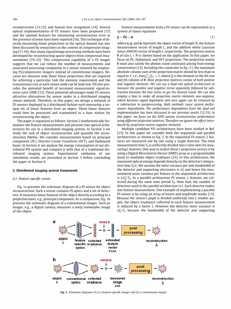
Fig. 1a presents the schematic diagram of a FS sensor for objectreconstruction. Such a sensor contains FS optics and a set of detec-tors. It measures linear features of the object directly according to aprojection basis, e.g., principal component. As a comparison, Fig. 1bpresents the schematic diagram of a conventional imager. Such animager, e.g., a digital camera, measures a noisy isomorphic imageof the object.

Fig. 1. Schematic diagrams of (a) a feature-spec

Feature measurements from a FS sensor can be represented as asystem of linear equations

y ¼ Fxþ n ð1Þ

where x, y, and n represent the object vector of length N, the featuremeasurement vector of length L, and the additive white Gaussiannoise (AWGN) vector of length L, respectively. The projection matrixF of size L � N is chosen based on the application. In this paper, wefocus on PC, Hadamard, and DCT projections. The projection matrixF must also satisfy the photon count constraint arising from energyconservation [12]. Including this constraint in Eq. (1), the maximumabsolute column sum of the projection matrix should be less than orequal to 1; i.e., maxj

Pijfijj 6 1, where fij is the element in the ith row

and jth column of F. Most projection matrices consist of both positiveand negative elements. We can use a dual-rail optical architecture tomeasure the positive and negative terms separately followed by sub-traction between the two terms to get the desired result. We can alsoemploy a bias to make all projection matrix elements non-negative,which becomes signal dependent and once again can be removed bya subtraction in postprocessing. Both methods cause system perfor-mance degradation. The performance degradation from the dual-railimplementation has been discussed in our previous works [12,15]. Inthis paper, we focus on the DFSI system reconstruction performanceusing different projection matrices. Therefore we ignore the effect intro-duced by projection matrix negative elements.

Multiple candidate FSI architectures have been studied in Ref.[15]. In this paper we consider both the sequential and parallelarchitectures as shown in Fig. 2. In the sequential FS sensor, L fea-tures are measured one by one using a single detector. The totalmeasurement time T0 is uniformly divided into L time slots for mea-suring L features. One way to realize these L projection vectors is byusing a Digital Micromirror Device (DMD) array as a programmablemask to modulate object irradiance [23]. In this architecture, themeasured optical energy depends linearly on the detector’s integra-tion time T0/L. We assume the noise variance per unit bandwidth ofthe detector and supporting electronics is r2

0 and hence the mea-surement noise variance per feature in the sequential architectureis Lr2

0=T0. In a parallel architecture FS sensor, L features are col-lected during the same time period T0. Note that, the number ofdetectors used in the parallel architecture is L. Each detector makesone feature measurement. One example of implementing a parallelFS sensor is by using an array of lenses and amplitude masks [15].Because the sensor’s pupil is divided uniformly into L smaller pu-pils, the object irradiance collected in each feature measurementis reduced by a factor L. However the detector noise variance isr2

0=T0 because the bandwidth of the detector and supporting

ific imager and (b) a conventional imager.

Fig. 2. Two implementations of a feature-specific imager using (a) sequential and (b) parallel architectures.

J. Ke et al. / Optics Communications 282 (2009) 185–197 187

electronics is 1=T0. Comparing the two architectures, the noise var-iance in the sequential architecture is L times larger than that in theparallel architecture. Therefore, we expect that the distributed FSI(DFSI) system using a parallel architecture will provide better per-formance than the sequential architecture.

In a conventional imager, optical resolution is often determinedusing the diffraction limit of the imaging optics and the camera’s sen-sor pixel size. However, in a FS sensor the concept of resolution is notwell-defined. The FS sensor makes non-conventional projective mea-surements as shown in Fig. 1a. Therefore the FS detector size doesnot have any direct impact on reconstruction resolution, hence wedo not define the measurement resolution. The reconstruction resolu-tion depends on the optics between the scene and the mask, the maskpixel size, and the number of feature measurements L. In this paper, weassume that this resolution is matched to the desired object pixel size.

2.2. Distributed Imaging System

Fig. 3 presents the schematic diagrams of two distributed imag-ing systems, each with K sensor units. A distributed conventional

Fig. 3. Schematic diagrams of (a) a distributed imaging system using conventional imageThe imagers in DCI measure different views of an object, whereas the imagers in DFSI m

imaging (DCI) system consisting of conventional imagers is shownin Fig. 3a. Each imager makes N measurements. Fig. 3b presents aDFSI system consisting of FS sensors. Each sensor makes L�N mea-surements. Therefore a total of, M = L � K features are measured in aDFSI system with K sensors. A sequential architecture DFSI system con-sists of K detectors, because features are measured one after the otherby the single detector in each sensor. A parallel architecture DFSI sys-tem consists of M detectors. Each sensor has L detectors to make fea-ture measurements during the same time period. In both DCI and DFSIsystems, sensor units send the measurements to a base stationafter some processing e.g. data compression. To simplify the prob-lem, we assume that the distance from object to sensor is large andthat the distances from different sensors to the base station areapproximately the same. However, the geometry of sensors mustbe taken into consideration during the design of the DFSI systemand during the postprocessing in a DCI system. Consider the DCIsystem as an example. Because each imager in the array of conven-tional imagers will have different positions and orientations, themeasured images will have different rotation angles, magnifica-tions, and translations. We choose one sensor as the reference.

rs (DCI), and (b) a distributed imaging system using feature-specific imagers (DFSI).easure different linear projections of the object.


Then the geometry of the kth sensor with respect to the referencecan be represented by a geometric transformation matrix Gk. Tocompensate for these geometric effects in a DFSI system, the samegeometric transformation is applied to the projection vectors dur-ing the system design and/or deployment. For example, in a DFSIsystem the feature measurements yk for the kth sensor can be writ-ten as

yk ¼ ðGkFTkÞ

T Gkxþ nk ) yk ¼ Fkxþ nk ð2Þ

where Gk is the N � N matrix representing the geometry of the kthimager, Fk is the L � N projection matrix required for measuring fea-tures in the kth imager, and nk is the L dimensional measurementnoise vector at the kth imager. In the next section, we discuss differ-ent types of Fk, a method to obtain an object estimate from the setof fyk; k ¼ 1;2; . . . ;Kg, and the reconstruction fidelity of the result-ing object estimates.

3. Reconstruction fidelity: simulation and analysis

We use the linear minimum mean squared error (LMMSE) esti-mation to reconstruct the object in a DFSI system. The LMMSE esti-mate is given by x̂ ¼Wy, where W is the Wiener operator definedas

W ¼ RxFTðFRxFT þ DnÞ�1 ð3ÞRx and Dn are the object and noise autocorrelation matrices,

respectively. Reconstruction fidelity is evaluated using of the root

mean squared error RMSE ¼ffiffiffiffiffiffiffiffiffiffiffiffiffiffiffiffiffiEfjx�x̂j2

N gq

where E is the ensembleaverage over many objects. Our fundamental object size is 32 � 32.We derive 1024-dimension projection vectors to work with the funda-mental object. However for training purpose we employ two hundred

0 20 40 60 80 100 120 140 1600.12

0.14

0.16

0.18

0.2

0.22

0.24

M

RM

SE

Parallel − PCAParallel − DCTParallel − HadamardSequential − PCASequential − DCTSequential − Hadamard

a

0 50 100 150 200 250 300 350 4000.1

0.11

0.12

0.13

0.14

0.15

0.16

M

RM

SE

c

Fig. 4. Plots of reconstruction RMSE versus the number of features M collected by sensimagers. The noise variance is r2

0 ¼ 0:1.

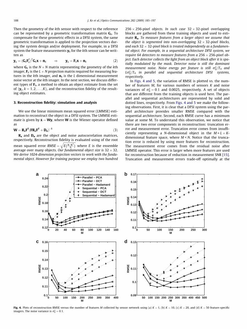
256 � 256-pixel objects. In such case 32 � 32-pixel overlappingblocks are gathered from these training objects and used to esti-mate Rx. To measure features from a larger object we assume thatthe object is segmented into non-overlapping 32 � 32-pixel blocks,and each 32 � 32-pixel block is treated independently as a fundamen-tal object. For example, in a sequential architecture DFSI system, werequire 64 detectors to measure features from a 256 � 256-pixel ob-ject. Each detector collects the light from an object block after it is spa-tially modulated by the mask. Detector noise is still the dominantmeasurement noise. Noise energy per feature is still r2

0=T0 andLr2

0=T0 in parallel and sequential architecture DFSI systems,respectively.

In Figs. 4 and 5, the variation of RMSE is plotted vs. the num-ber of features M, for various numbers of sensors K and noisevariances of r2

0 ¼ 0:1 and 0.0025, respectively. A set of objectsthat are different from the training objects is used here. The par-allel and sequential architectures are represented by solid anddotted lines, respectively. From Figs. 4 and 5 we make the follow-ing observations. First, it is clear that a DFSI system using the par-allel architecture provides smaller RMSE compared with thesequential architecture. Second, each RMSE curve has a minimumvalue at some M. To understand this observation, we notice thatthere are two error components in reconstruction: truncation er-ror and measurement error. Truncation error comes from insuffi-ciently representing a N-dimensional object in the M = L � K-dimensional feature space, where M < N. Notice that the trunca-tion error is reduced by using more features for reconstruction.The measurement error comes from the residual noise afterLMMSE operator. This error is larger when more features are usedfor reconstruction because of reduction in measurement SNR [15].Truncation and measurement errors trade-off optimally at the

0 50 100 150 200 250 3000.1

0.11

0.12

0.13

0.14

0.15

0.16

0.17

M

RM

SE

b

50 100 150 200 250 300 350 400 450 5000.09

0.1

0.11

0.12

0.13

M

RM

SE

d

or network using (a) K ¼ 1, (b) K ¼ 10, (c) K ¼ 20, and (d) K ¼ 50 feature-specific

0 20 40 60 80 100 120 140 160 180 2000.1

0.12

0.14

0.16

0.18

0.2

0.22

M

RM

SE


a

0 50 100 150 200 250 300 350 400 450 5000.09

0.1

0.11

0.12

0.13

0.14

0.15

M

RM

SE

b

0 100 200 300 400 500 6000.08

0.085

0.09

0.095

0.1

0.105

0.11

0.115

0.12

0.125

0.13

M

RM

SE

c

0 100 200 300 400 500 600 700 800 900 10000.06

0.07

0.08

0.09

0.1

0.11

0.12

M

RM

SE

d

Fig. 5. Plots of reconstruction RMSE versus the number of features M collected by sensor network using (a) K ¼ 1, (b) K ¼ 10, (c) K ¼ 20, and (d) K ¼ 50 feature-specificimagers. The noise variance is r2

0 ¼ 0:0025.

Fig. 6. Example reconstructions using PCA projections from K ¼ 10 number ofimagers at noise level of r2

0 ¼ 0:0001. (a) Object of size 32� 32. Reconstructionsusing sequential architecture with (b) M = 200, and (c) M = 500 features. Recon-struction using parallel architecture with (d) M = 200, and (e) M = 500 features.


minimum RMSE point. The third observation is that comparedwith the DCT and Hadamard bases, the PCA basis achieves smal-ler RMSE value when M is small. For example, the RMSE valuesusing PCA, Hadamard, and DCT features are 0.0974, 0.1022, and0.1055, respectively when M = 100, K = 50, and r2

0 ¼ 0:1. Becausethe PCA bases are derived from Rx which corresponds to objectprior knowledge, they can yield smaller truncation error andRMSE when M is small (i.e., when truncation error dominates).This also means that the PCA projection achieves its minimumRMSE value using a smaller M value. However, when M is large,reconstruction using the Hadamard features has smaller RMSE.For example, the RMSE values using PCA, Hadamard, and DCT fea-tures are 0.1102, 0.0984, and 0.1036, respectively when M is in-creased to 500, and keeping K = 50, and r2

0 ¼ 0:1. Becausemeasurement error dominates RMSE when M is large, it is morecritical to increase the signal energy (hence the measurementSNR) than to use a basis with a good data compaction property.Collecting more photons requires that all column sums of F bemade close to 1 after normalization in order to minimize photonloss. The Hadamard basis satisfies this requirement, and hencethe Hadamard based DFSI system has smaller measurement errorwith large M. We also observe that the minimum reconstructionRMSE reduces with increasing number of imagers, K. For examplefrom Fig. 4 we notice that the minimum RMSE decreased from0.124 to 0.095 when K is increased from 1 to 50 in case of parallelHadamard implementation. In fact this trend holds when K isincreased for a fixed M. Fig. 6 presents examples of an object andsome reconstructions. The projection method is PCA, the number ofimagers K = 10, and noise variance r2

0 ¼ 0:0001. The RMSE valuesobtained from the sequential architecture DFSI system are 0.1108and 0.1233 for M = 200 and 500, respectively. These values are higherthan the RMSE values obtained from the parallel architecture DFSI

system, which are 0.1027 and 0.0867 when M = 200 and 500,respectively.

We extract the minimum RMSE values from Figs. 4 and 5 andplot them as a function of noise variance in Fig. 7. The followingobservations are based on Fig. 7. 1) As expected, the parallel DFSIsystem exhibits better RMSE performance at all noise levels. 2)When the noise level is high, reconstruction using the PCA andHadamard features provide similar RMSE performance. 3) Whenthe noise level is small, e.g., r2

0 < 10�6 and K = 50 as in Fig. 7d,reconstruction using the PCA basis has slightly smaller RMSE,

10−8

10−6

10−4

10−2

100

0

0.02

0.04

0.06

0.08

0.1

0.12

0.14

0.16

σ02

min

imu

m R

MS

E


10−8

10−6

10−4

10−2

100

0

0.02

0.04

0.06

0.08

0.1

0.12

0.14

σ02

min

imu

m R

MS

E

10−8

10−6

10−4

10−2

100

0

0.02

0.04

0.06

0.08

0.1

0.12

σ02

min

imu

m R

MS

E

10−8

10−6

10−4

10−2

100

0.02

0.04

0.06

0.08

0.1

σ02

min

imu

m R

MS

E

a b

c d

Fig. 7. Minimum reconstruction RMSE versus the noise variance r20 for sensor network with (a) K ¼ 1, (b) K ¼ 10, (c) K ¼ 20, and (d) K ¼ 50 feature-specific imagers.


because the PCA is optimal in the absence of noise. 4) When thenoise level is in the moderate range, the Hadamard basis providessmaller minimum RMSE. As described before, this is because onaverage more object photons will be collected using Hadamard fea-tures. Therefore, making more Hadmard feature measurementswill reduce the truncation error with minimal increase in the mea-surement error.

0 5 10 15 200

100

200

300

400

500

600

700

800

900

1000

Mo

pt

PCA, σ02 = 0.8

DCT, σ02 = 0.8

Hadamard, σ02 = 0.8

PCA, σ02 = 0.01

DCT, σ02 = 0.01


PCA, σ02 = 0.0025

DCT, σ02 = 0.0025


Fig. 8. The number of features generating minimum RMSE, Mopt , versus the number of imand 0:0025.

Next we examine the optimal number of features Mopt requiredto achieve the minimum RMSE. Fig. 8 plots Mopt as a function of Kfor three different noise levels r2

0 ¼ 0:8, 0.01, and 0.0025. PCA,Hadamard, and DCT features are studied. Only the parallel DFSIarchitecture is discussed here onwards because of its superiorRMSE performance. From Fig. 8, it is clear that Mopt increases withincreasing K or decreasing r2

0. This is because increasing K and/or

25 30 35 40 45 50K

agers in a DFSI sensor network, K. Data is shown for three noise levels r20 = 0:8, 0:01,

0 5 10 15 20 25 30 35 40 45 500

0.02

0.04

0.06

0.08

0.1

0.12

0.14

0.16

0.18

K

min

inu

m R

MS

E

PCA, σ

02 = 0.8

DCT, σ02 = 0.8


PCA, σ02 = 10−4

DCT, σ02 = 10−4

Hadamard, σ02 = 10−4

PCA, σ02 = 10−6

DCT, σ02 = 10−6

Hadamard, σ02 = 10−6

Fig. 9. Minimum reconstruction error versus the number of imagers K in a DFSI sensor network. Data is shown for three noise levels r20 = 0:8, 10�4, and 10�6.

Fig. 10. Compression protocol used for FS imagers. The quantization table isdifferent for different types of measured features.


reducing r20 improves the measurement SNR. When measurement

SNR increases, a larger number of features can be measured beforebalance of noise and truncation error is reached. Fig. 8 also demon-strates that Hadamard basis vectors generally require the largestMopt values to achieve minimum RMSE.

The last aspect of DFSI reconstruction performance is the im-pact of the number of imagers K on reconstruction quality. Fig. 9presents the minimum RMSE versus K for high, moderate, andlow noise levels using PCA, DCT, and Hadamard features. As ex-pected, the minimum RMSE decreases as more FS imagers are usedand/or as the detector noise level r2

0 is reduced.

4. System lifetime: simulation and analysis

In this section we quantify the lifetime of a distributed imagingsystem by calculating its energy consumption. The system lifetimeis expected to be short when the energy consumption is high, andvice-versa. We define the DFSI system lifetime as the maximumtime period before any one FS imager runs out of battery. This def-inition is sensible because in a DFSI system, all sensors work in col-laboration to measure the scene. In a DCI system on the other hand,at any given time only one conventional imager is assumed to be inthe active mode for measuring, compressing, and transmittingdata. After one such imager runs out of battery, another imageris turned on. Therefore the DCI system lifetime is the time periodbefore all imagers run out of battery.

Three processes dominate the energy consumption in adistributed imaging system: the energy used for (1) measurementEmeas, (2) on-board processing/data compression Eproc, and (3)communication Ecomm. We calculate these three energy compo-nents by considering commercially available electronics and opti-cal devices for the proof of concept. The power consumptiondetails of these devices are discussed in the Appendix. Summingup all three values Emeas, Eproc, and Ecomm gives the total energyconsumption for one imager. Then, the lifetimes of DCI and DFSIsystems are defined as

DCI Lifetime ¼ Eb

Econv� K ðroundÞ ð4Þ

DFSI Lifetime ¼ Eb

maxkfEkFSg

ðroundÞ ð5Þ

where Eb is the sensor battery energy, Econv is the energy consump-tion for one conventional imager, and Ek

FS is the total energy con-sumption for the kth FS sensor. We assume that in each time unitsensors measure, process, and send data back to the base station forsingle object. In our study, we use a previously defined time unit ofround to quantify the system lifetime [24]. We assume that one Ener-gizer 186 button cell battery is used for the sensor power supply. Itcan provide roughly 500 J of energy before its working voltagedrops below the cut-off value 0.9 V.

We use 7 objects of size 480 � 640-pixels to evaluate DFSI andDCI energy consumption. They are processed block-wise using32 � 32-pixel blocks as described in Section 3. Both systems haveK = 20 imagers. We consider the noise level of r2

0 ¼ 0:04.Note that an important part of the on-board processing is the

compression of the measurements before sending them to the basestation. Fig. 10 presents the compression protocol used in our DFSIsystem. The details of the protocols used in both systems are in-cluded in the Appendix. Here we elaborate on the effect of quanti-zation on the DFSI reconstruction process. The measured features

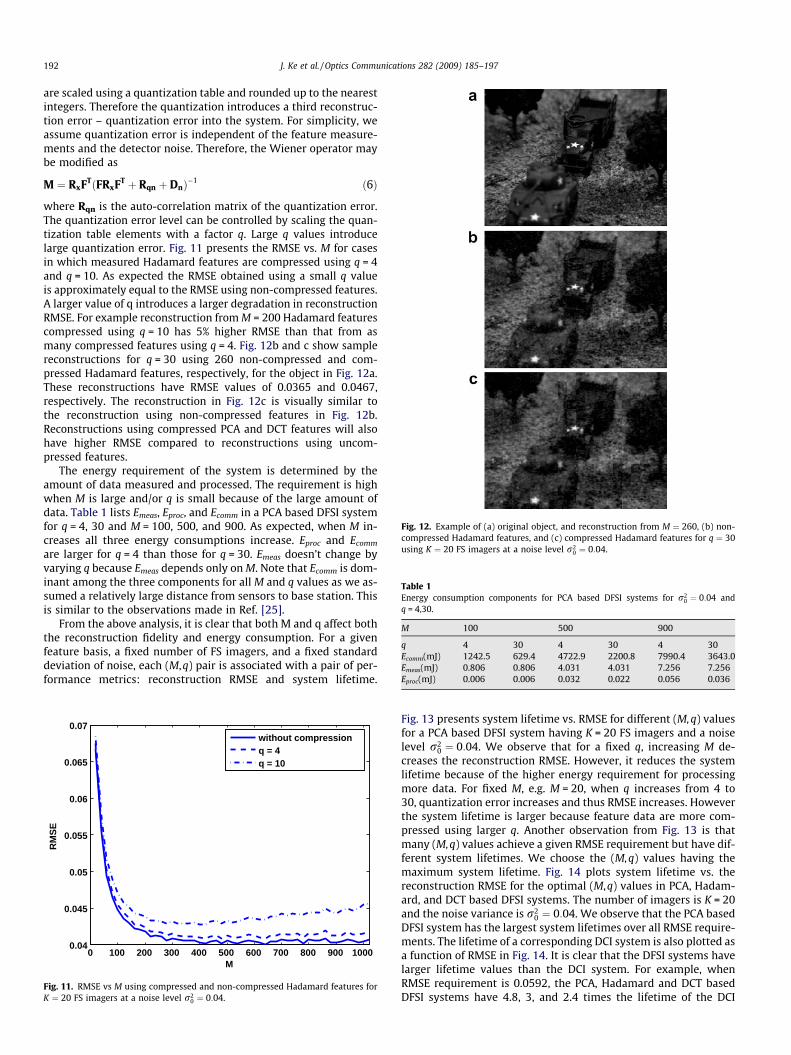
Fig. 12. Example of (a) original object, and reconstruction from M ¼ 260, (b) non-compressed Hadamard features, and (c) compressed Hadamard features for q ¼ 30using K ¼ 20 FS imagers at a noise level r2

0 ¼ 0:04.

Table 1Energy consumption components for PCA based DFSI systems for r2

0 ¼ 0:04 andq = 4,30.

M 100 500 900

q 4 30 4 30 4 30Ecomm(mJ) 1242.5 629.4 4722.9 2200.8 7990.4 3643.0Emeas(mJ) 0.806 0.806 4.031 4.031 7.256 7.256Eproc(mJ) 0.006 0.006 0.032 0.022 0.056 0.036


are scaled using a quantization table and rounded up to the nearestintegers. Therefore the quantization introduces a third reconstruc-tion error – quantization error into the system. For simplicity, weassume quantization error is independent of the feature measure-ments and the detector noise. Therefore, the Wiener operator maybe modified as

M ¼ RxFTðFRxFT þ Rqn þ DnÞ�1 ð6Þ

where Rqn is the auto-correlation matrix of the quantization error.The quantization error level can be controlled by scaling the quan-tization table elements with a factor q. Large q values introducelarge quantization error. Fig. 11 presents the RMSE vs. M for casesin which measured Hadamard features are compressed using q = 4and q = 10. As expected the RMSE obtained using a small q valueis approximately equal to the RMSE using non-compressed features.A larger value of q introduces a larger degradation in reconstructionRMSE. For example reconstruction from M = 200 Hadamard featurescompressed using q = 10 has 5% higher RMSE than that from asmany compressed features using q = 4. Fig. 12b and c show samplereconstructions for q = 30 using 260 non-compressed and com-pressed Hadamard features, respectively, for the object in Fig. 12a.These reconstructions have RMSE values of 0.0365 and 0.0467,respectively. The reconstruction in Fig. 12c is visually similar tothe reconstruction using non-compressed features in Fig. 12b.Reconstructions using compressed PCA and DCT features will alsohave higher RMSE compared to reconstructions using uncom-pressed features.

The energy requirement of the system is determined by theamount of data measured and processed. The requirement is highwhen M is large and/or q is small because of the large amount ofdata. Table 1 lists Emeas, Eproc, and Ecomm in a PCA based DFSI systemfor q = 4, 30 and M = 100, 500, and 900. As expected, when M in-creases all three energy consumptions increase. Eproc and Ecomm

are larger for q = 4 than those for q = 30. Emeas doesn’t change byvarying q because Emeas depends only on M. Note that Ecomm is dom-inant among the three components for all M and q values as we as-sumed a relatively large distance from sensors to base station. Thisis similar to the observations made in Ref. [25].

From the above analysis, it is clear that both M and q affect boththe reconstruction fidelity and energy consumption. For a givenfeature basis, a fixed number of FS imagers, and a fixed standarddeviation of noise, each (M,q) pair is associated with a pair of per-formance metrics: reconstruction RMSE and system lifetime.

0 100 200 300 400 500 600 700 800 900 10000.04

0.045

0.05

0.055

0.06

0.065

0.07

M

RM

SE

without compressionq = 4q = 10

Fig. 11. RMSE vs M using compressed and non-compressed Hadamard features forK ¼ 20 FS imagers at a noise level r2

0 ¼ 0:04.

Fig. 13 presents system lifetime vs. RMSE for different (M,q) valuesfor a PCA based DFSI system having K = 20 FS imagers and a noiselevel r2

0 ¼ 0:04. We observe that for a fixed q, increasing M de-creases the reconstruction RMSE. However, it reduces the systemlifetime because of the higher energy requirement for processingmore data. For fixed M, e.g. M = 20, when q increases from 4 to30, quantization error increases and thus RMSE increases. Howeverthe system lifetime is larger because feature data are more com-pressed using larger q. Another observation from Fig. 13 is thatmany (M,q) values achieve a given RMSE requirement but have dif-ferent system lifetimes. We choose the (M,q) values having themaximum system lifetime. Fig. 14 plots system lifetime vs. thereconstruction RMSE for the optimal (M,q) values in PCA, Hadam-ard, and DCT based DFSI systems. The number of imagers is K = 20and the noise variance is r2

0 ¼ 0:04. We observe that the PCA basedDFSI system has the largest system lifetimes over all RMSE require-ments. The lifetime of a corresponding DCI system is also plotted asa function of RMSE in Fig. 14. It is clear that the DFSI systems havelarger lifetime values than the DCI system. For example, whenRMSE requirement is 0.0592, the PCA, Hadamard and DCT basedDFSI systems have 4.8, 3, and 2.4 times the lifetime of the DCI

0.04 0.045 0.05 0.055 0.06500

1000

1500

2000

RMSE

Lif

etim

e (r

ou

nd

s)

q = 4q = 10q = 20q = 30M = 20M = 40M = 60

(20,30)

(M,q)

(60,4)

(60,30)

(60,20)

(60,10)

(20,4)

(20,10)

(20,20)

Fig. 13. Lifetimes of PCA based DFSI system with noise level r20 ¼ 0:04 for different

(M,q)).

0.03 0.04 0.05 0.06 0.07 0.08 0.090

500

1000

1500

2000

2500

RMSE

Lif

etim

e (r

ou

nd

s)

PCAHadamardDCTDCI

Fig. 14. Lifetimes of DCI system and DFSI system using PCA, DCT and Hadamardfeatures with noise level r2

0 ¼ 0:04 when (M; q) is optimized.

Fig. 15. A snapshot of DFSI experimental set-up.


system, respectively. More imagers can be used to further improvethe DFSI system lifetime.

5. Experiment

We used a conventional distributed imaging setup in order tovalidate the simulation results obtained from our DFSI systemmodel. Fig. 15 shows a snapshot of the experimental setup. Theplasma monitor is used to display an object at a distance of about1.5 m from an array of Firewire-based web-cameras and imageswith different views of the object are captured. The cameras areplaced at the same distance from the object and an affine geometryis assumed for their deployment. The rotation, magnification, andtranslation parameters of each camera are determined during the sys-tem calibration. A grid patterned image is shown on the monitor as acalibration object. The camera parameters are estimated by matchingthe image with respect the reference image. The image calibration isperformed by choosing a set of corresponding points in the image tobe aligned and reference image [26]. The difference between the refer-

ence and the calibration result is very small. The process of featuremeasurement is emulated numerically using these measuredimages. These features are further corrupted by additive whiteGaussian noise. We consider PCA, DCT, and Hadamard featuresassuming the parallel FSI architecture. The noise variance isr2

0 ¼ 0:09. In Fig. 16 we plot RMSE vs. M using K = 2,3, and 4 imag-ers and a 128 � 128-pixel object. As mentioned in Section 3, weprocess the object as a set of 32 � 32-pixel blocks. For each blockwe make L = M/K feature measurements. With accurate knowledgeof all camera geometries, the experimental RMSE curves can be ex-pected to behave in the same way as did the simulation RMSEcurves. From Fig. 16 we observe that the reconstruction RMSE re-duces with increasing K. The experimental data also exhibits aminimum RMSE at Mopt. The optimal number of features at whichthis minimum is achieved increases with increasing K as shown inTable 2. The table also lists the minimum RMSE values and the Mopt

values obtained by using only one captured image and simulatingthe remaining images by numerically performing the geometrictransformations. We find that the minimum RMSE values matchvery well and that the experimental system generally requires afew more features to achieve the same RMSE. Some examplereconstructions using PCA and Hadamard features are shown inFig. 17. Fig. 17a and e show images captured using two conven-tional cameras from which FSI performance is emulated. Theimages in Fig. 17b–d are reconstructed using 36 PCA features fromK = 2, 3, and 4 cameras, respectively. They have RMSE values of0.119, 0.111, and 0.105, respectively. The images in Fig. 17f–h arereconstructed using 120 Hadamard features using K = 2, 3, and 4cameras, respectively. These images have RMSE values of 0.151,0.136, and 0.126, respectively. As K increases both the RMSE andthe visual quality of reconstructions improve. As we discussed inthe previous section, the resolution concept is not well-defined in DFSIsystem. We assume that the optical resolution is matched to the de-sired object pixel size.

We extend our experiments to include evaluations of energyconsumption and lifetime as explained in Section 4. Fig. 18 showsreconstruction RMSE versus the total number of features usingK = 5 imagers with compressed and uncompressed PCA, Hadamard,and DCT features. In the case of compression we used a quantiza-tion table with a scaling factor q = 10. We observe that compres-sion degrades the reconstruction fidelity. For example thereconstruction RMSE increases by 7.8%, 11.4%, and 19.4% due tocompressing 200 DCT, Hadamard, and PCA features, respectively.Next we quantify the lifetime of the system. Because there aremany (M,q) values that achieve a required reconstruction RMSEwe conduct an exhaustive search to find the optimal pair for eachRMSE. Fig. 19 plots DFSI system lifetime obtained by using the

0 50 100 150 200 250 300 350 400 450 5000.1

0.12

0.14

0.16

0.18

0.2

0.22

0.24

0.26

0.28

M

K=2K=4

PCADCTHadamard

RM

SE

Fig. 16. The reconstruction RMSE versus the total number of PCA features and Hadamard features using K ¼ 2, 3, and 4 cameras. The noise variance is r20 ¼ 0:09.

Table 2Mopt for K = 2,3,4 using PCA, Hadamard, and DCT features.

Simulation Experiment

PCA Hadamard DCT PCA Hadamard DCT

min RMSE Mopt min RMSE Mopt min RMSE Mopt min RMSE Mopt min RMSE Mopt min RMSE Mopt

K = 2 0.114 22 0.150 114 0.163 86 0.114 22 0.150 98 0.163 88K = 3 0.108 22 0.134 117 0.150 87 0.109 30 0.136 135 0.150 90K = 4 0.104 22 0.125 124 0.140 92 0.104 32 0.126 164 0.140 98

Fig. 17. Example reconstructed images. Images obtained from two conventional cameras are shown in (a) and (e). The images in (b), (c), and (d) are reconstructed using 36PCA features and K ¼ 2, 3, and 4 cameras, respectively. The images in (f), (g), and (h) are reconstructed using 120 Hadamard features and K ¼ 2, 3, and 4 cameras. The noisevariance r2

0 ¼ 0:09.


optimal (M,q) values versus the achieved reconstruction RMSE forK = 5 imagers. We also compare the lifetimes of DFSI systems usingHadamard, PCA, DCT with that of a corresponding DCI system. The

DFSI system measuring PCA features has the highest lifetime for afixed reconstruction RMSE because of its lowest energy require-ment to achieve given reconstruction fidelity. The DCT and Hadam-

0 100 200 300 400 500 600 700 800 900 10000.1

0.12

0.14

0.16

0.18

0.2

0.22

0.24

0.26

0.28

0.3

M

RM

SE

PCA − no compressionPCA − compressionDCT − no compressionDCT − compressionHadamard − no compressionHadamard − compression

Fig. 18. RMSE versus the total number of features M with or without compressing PCA, DCT, and Hadamard features. The number of cameras K ¼ 5 and noise variancer2

0 ¼ 0:09. The compression scaling factor q ¼ 10.

0.12 0.13 0.14 0.15 0.16 0.17 0.18 0.19 0.2

103

104

RMSE

Lif

etim

e (r

ou

nd

s)

HadamardPCADCTDCI

Fig. 19. Lifetimes of DCI system and DFSI systems using Hadamard, PCA, and DCT features versus the achieved reconstruction RMSE. The optimal (M,q) pair is chosen at everyRMSE. The number of imagers K ¼ 5 and the noise variance r2

0 ¼ 0:09.

Table 3Energy consumption components for DCI and DFSI systems.

DCI DFSI

Featuremeasurement

Equipment OmniVision OV7141 Thorlab DET10A &TLC1541

Emeas 1.3 mJ/sensor 0:5375LlJ/sensorOn-board process Equipment ARM7TDMI ARM7TDMI

Ecomp ð1100N þ 4000NnÞ pJ/sensor

ð200Lþ 4000aÞ pJ/sensor

Transmission Ecomm 100;050c nJ/sensor 100; 050c nJ/sensor

* N is the number of object pixels; L is the number of features for each sensor; n isthe compression quality; a is the number of non-zeros coefficients after compres-sion; c is the amount of transmission data in bits.


ard features yield almost the same lifetime. The lifetimes of DFSIsystems using PCA, Hadamard, and DCT features are 20.2�, 8.4�and 7.2� higher than the lifetime of DCI system, respectively atRMSE of 0.149.

6. Conclusion

In this paper we present the concept of a distributed imagingsystem that consists of FS imagers to collect data for object recon-struction. We consider PCA, Hadamard, and DCT features usingeither the sequential or the parallel optical implementationschemes. Reconstruction fidelity quantified using RMSE, is


analyzed for systems with different numbers of imagers (K) formeasuring different total numbers of features (M) at several mea-surement noise levels, r0. We observe that the parallel architectureprovides better reconstruction fidelity than the sequential archi-tecture. We find that the RMSE of reconstructed images reducessignificantly for K > 1 imagers. PCA offers the best reconstructionfidelity for measuring small M at all noise levels, and also for largeM at very low noise level. At high noise levels, e.g., r0 > 0:1, bothPCA and Hadamard features perform equally well in terms of min-imum RMSE. At moderate noise levels measuring Hadamard fea-tures is beneficial.

We also analyze the lifetime of a distributed sensor network. Asimple communication protocol is assumed and data sheets fromcommercially available hardware are used to calculate energy con-sumption in the system. We compare energy consumption andlifetime of a DFSI system with those of a DCI system both havingthe same number of sensors. The measurement, computation,and transmission costs are calculated to obtain the total energyconsumption in both systems, and by using these data, lifetimesare determined. The lifetime of the DFSI system is 4.8� that ofthe DCI system when both systems have 20 imagers, reconstruc-tion RMSE requirement is 6%, and the noise level r0 ¼ 0:2. To val-idate reconstruction fidelity and lifetime observations from thesimulations, we emulate a DFSI system by using an array of 5 con-ventional cameras deployed in an affine geometry. We observesimilar trends in systems performance.

Appendix A. Energy consumption calculation

Here we discuss the computation of three energy consumptioncomponents: Emeas, Eproc, and Ecomm.

A.1. The measurement energy consumption Emeas

In a DCI system, we assume an OmniVision VGA camera chipOV7141 and conventional imaging optics to make an isomorphicmeasurement of the object. The chip has power consumption of40mW in active mode and frame rate of 30 fps. Therefore Emeas ina DCI system using OV7141 is 1.33 mJ per frame.

The calculation of Emeas in a DFSI system is different from that ina DCI system. A Thorlabs high speed silicon detector DET10A is as-sumed to collect feature values. Following this detector is a 10-bitsanalog-to-digital converter (ADC) TLC1541 from Texas InstrumentInc. The power consumption of DET10A is defined as P = I2R, where Iis the photocurrent of the detector, R is the resistance of the circuit.According to the manual of DET10A, there is a 1 kX equivalentresistor in the detector and a recommended 50X load resistor.We assume an average photocurrent I is 0.1 mA for visible light.Using the same data sampling rate of 30 fps as in the DCI system,the energy consumption for measuring one feature using a DET10Adetector is 0.35 lJ. Adding the ADC energy consumption from itsdata sheet, the total energy used to measure one feature in DFSIsystem is 0.5375 lJ. If one FS imager measures L features, thenEmeas for one FS imager is 0.5375L lJ.

A.2. The on-board processing energy consumption Eproc

Eproc is the energy required for compressing the measurements.We assume an ARM7TDMI microprocessor for implementing datacompression in both systems. The time period for accomplishing1 multiplication, addition, and comparison each is 4, 1, and 1microprocessor operation clock cycles, respectively. The energyused in one clock cycle is 50 pJ. In a DCI system, we use JPEG stan-dard [27,28] for data compression. The DCT-based compression inJPEG standard consists of 8 � 8 DCT transformation, quantization

and Huffman coding. According to Prisch et al. [29], the computa-tion requirement for l � l DCT is log2l multiplications and 2log2l

additions for each pixel using the fast algorithm. The computationcost for quantization is 1 multiplication per pixel. Therefore, theenergy for accomplishing 8 � 8 DCT transformation and quantiza-tion process for a

ffiffiffiffiNp�

ffiffiffiffiNp

-pixel object is (3 (multiplica-tion) � 4 + 6 (addition) + 1(multiplication) � 4) �N � 50 = 1100NpJ. The Huffman coding procedure is basically a search procedureover a lookup table. On average half of the table or 80 elementswill be searched to code one non-zero DCT coefficient [28].Therefore, the energy consumed for Huffman coding a

ffiffiffiffiNp�ffiffiffiffi

Np

-pixel object is 4000Nn pJ, where n is the compression qualityvarying from 0 to 1. Now we can formulate Eproc for one imager inDCI system as ð1100N þ 4000NnÞ pJ.

In a DFSI system, the measured data are feature values or trans-formation coefficients directly. Therefore, transformation compu-tation is saved in the DFSI system. However, the feature valuesneed to be quantized and coded before transmission. Fig. 10 showsthe proposed compression protocol for DFSI system. We use thesame Huffman coding procedure as in JPEG. The quantization ta-bles Q are designed individually for each transformation. For DCTfeatures, we interpolate the 8 � 8 DCT quantization table Q DCT

8 inJPEG to generate the 32 � 32 quantization table Q DCT

32 . For PCAand Hadamard features, we design the quantization tables Q PCA

32

and Q Hadamard32 based on the eigen-values of Rx. Eproc for one FS ima-

ger in a DFSI system is defined as ð200Lþ 4000aÞ pJ, where a is thenumber of non-zeros coefficients after compression.

A.3. The communication energy consumption Ecomm

Ecomm is modeled as Ecommðc; dÞ ¼ Eeleccþ eampcd2, where Eelec =50 nJ/bit is the radio dissipate, eamp ¼ 100pJ=ðbit �m2Þ is for thetransmitter amplifier, c is the number of data bits transmitted,and d is the transmission distance [30]. All imagers are assumed1 km away from the base station. Therefore to transmit c data bits,Ecomm is 100;050cnJ.

Table 3 summarizes the device part numbers and energy con-sumption values for DCI and DFSI systems.

References

[1] Y. Sankarasubramaniam, I. Akyildiz, W. Su, E. Cayirci, IEEE CommunicationMagazine 40 (2002) 102.

[2] M. Rahimi, Y. Yu, D. Estrin, G.J. Pottie, M. Srivastava, G. Sukhatme, R. Pon, M.Batalin W.J. Kaiser, in: Proceedings 10th IEEE International Workshop onFuture Trends of Distributed Computing Systems, 2004, p. 102.

[3] S. Hengstler, H. Aghajan, in: Testbeds and Research Infrastructures for theDevelopment of Networks and Communities, IEEE, 2006.

[4] W. Feng, W. Feng, E. Kaiser, M. Baillif, Communications and Applications 1(2005) 151.

[5] Y. Liu, S. Das, IEEE Communication Magazine 44 (2006) 142.[6] S. Hengstler, H. Aghajan, ACM/IEEE International Conference on Distributed

Smart Cameras 1 (2007) 12.[7] E. Culurciello, A.G. Andreou, Analog Integrated Circuits and Signal Processing

49 (2006) 39.[8] D. Ganesan, G. Mathur, P. Desnoyers, P. Shenoy, in: Proceedings of the Fifth

International Conference on Information Processing in Sensor Networks, 2006,p. 374.

[9] M.W. Marcellin, J.C. Dagher, M.A. Neifeld, IEEE Transaction on ImageProcessing 15 (2006) 1705.

[10] C. Duran-Faundez, V. Lecuire, N. Krommenacker, EURASIP Journal on Imageand Video Processing (2007) 1.

[11] A. Savvides, E. Culurciello, in: 2nd International Conference on BroadbandNetworks. IEEE, 2005.

[12] M.A. Neifeld, P.M. Shankar, Feature Specific Imaging Applied Optics 42 (2003)3379.

[13] H. Pal, M.A. Neifeld, Optics Express 11 (2003) 2118.[14] H. Pal, D. Ganotra, M.A. Neifeld, Applied Optics 44 (2005) 3784.[15] M.A. Neifeld, J. Ke, Applied Optics 46 (2007) 5293.[16] J. Ke, M. Stenner, M.A. Neifeld, in: Proceedings of SPIE, Visual Information

Processing XIV, vol. 5817. SPIE, 2005.[17] D.J. Brady, N.P. Pitsianis, X. Sun, in: Proceedings of SPIE, Visual Information

Processing XIV, vol. 5817. SPIE, 2005.


[18] A. Portnoy, X. Sun, T. Suleski, M.A. Fiddy, M.R. Feldman, N.P. Pitsianis, D.J.Brady, R.D. TeKolste, in: Proceedings of SPIE, Intelligent IntegratedMicrosystems, vol. 6232. SPIE, 2006.

[19] D. Donoho, IEEE Transaction on Information Theory 52 (2006) 1289.[20] J.K. Romberg, E.J. Candes, Proceedings of SPIE, Wavelet Applications in Signal

and Image Processing XI, vol. 5914. SPIE, 2004.[21] E.J. Candes, in: Proceedings of the International Congress of Mathematicians,

2006.[22] J.A. Tropp, IEEE Transactions on Information Theory 50 (2004) 2231.[23] D. Takhar, J. Laska, T. Sun, K. Kelly, M. Duarte, M. Davenport, R. Baraniuk, To

appear in IEEE Signal Processing Magazine (2008).[24] K. Dasgupta, K. Kalpakis, P. Namjoshi, Computer Networks 42 (2003) 697716.

[25] V. Paciello L. Ferrigno, S. Marano, A. Pietrosanto, in: IEEE InternationalConference on Virtual Environments, Human–Computer Interfaces, andMeasurement Systems, 2005.

[26] A. Goshtasby, Image Visbile Computation 6 (1988) 255.[27] G.K. Wallace, Communications of the ACM 34 (1991) 30.[28] CCITT. Information technology – digital compression and coding of

continuous-tone still images – requirements and guidelines. ISO/IEC 10918-1:1993(E).

[29] N. Demassieux, P. Pirsch, W. Gehrke, Proceedings of the IEEE 83 (1995)220.

[30] S.S. Iyengar, R.R. Brooks, Distributed Sensor Networks, Chapman & Hall/CRC,2005.

distributed imaging using an array of compressive cameras

Documents