DISTRIBUTED DETECTION AND DATA FUSION IN RESOURCE CONSTRAINED WIRELESS SENSOR NETWORKS

A Thesis by

Bhavani Garimella

Bachelor of Technology, JNT University, Kakinada, 2001

Submitted to the College of Engineering and the faculty of the Graduate School of

Wichita State University in partial fulfillment of the requirements for the degree of

Masters of Science

December 2005

DISTRIBUTED DETECTION AND DATA FUSION IN RESOURCE CONSTRAINED WIRELESS SENSOR NETWORKS

I have examined the final copy of this thesis for form and content and recommend that it be accepted in partial fulfillment of the requirements for the degree of Master of Science, with a major in Electrical Engineering. ------------------------------------------------------------------ Dr. Sudharman K. Jayaweera, Committee Chair We have read this thesis and recommend its acceptance: ------------------------------------------------------------------ Dr. Coskun Cetinkaya, Committee Member ------------------------------------------------------------------ Dr. Krishna Krishnan, Committee Member

ii

DEDICATION

Dedicated to My Beloved Parents

iii

ACKNOWLEDGEMENTS

I would like to extend my sincere thanks to my graduate advisor Dr. Sudharman K.

Jayaweera for all his guidance and motivation not just academically but also morally. I would

like to thank Dr. Coskun Cetinkaya and Dr. Krishna Krishnan for being on my committee and

taking the pains to go through the thesis.

I sincerely thank my parents, Suresh Kandula and Bapu Garimella for their

unconditional love and sustained support through all the times. I owe a special gratitude to

Mr. and Mrs. Chalapathi Emani for their affection. I appreciate all my friends and roommates

at Wichita State for their valuable suggestions and support.

iv

ABSTRACT

Wireless sensor networks have received immense attention in recent years due to their

possible applications in various fields like battery-field surveillance, disaster recovery etc.

Since these networks are mostly resource-constrained there is a need for efficient algorithms

in maximizing the network resources. In this thesis, energy and bandwidth-efficient detection

and fusion algorithms for such resource constrained wireless sensor systems are developed. A

Sequential Probability Ratio Test (SPRT) based detection algorithms for an energy-

constrained sensor network is proposed. Performance is evaluated in terms of number of

nodes required to achieve a given probability of detection. Simulation results show that a

network implementing the SPRT based model outperforms a network having a parallel fusion

detector. To implement distributed detection and fusion in energy and bandwidth constrained

networks, non-orthogonal communication is considered to be one of the possible solutions.

An optimal Bayesian data fusion receiver for a DS-CDMA based distributed wireless sensor

network having a parallel architecture is proposed. It is shown that the optimal Bayesian

receiver outperforms the partitioned receivers in terms of probability of error. But the

complexity of this optimal receiver is exponential in the number of nodes. In order to reduce

the complexity, partitioned receivers that perform detection and fusion in two stages are

proposed. Several well-known multi-user detectors namely, JML, matched filter, Decorrelator

and linear MMSE detectors are considered for the first stage detection and performance is

evaluated in terms of probability of error at the fusion center. Conventional detector based

fusion receiver has a performance close to that of optimal fusion receiver with quite less

complexity under specific channel conditions. Performance and complexity trade-offs should

be considered while designing the network.

v

TABLE OF CONTENTS

Page

1 Introduction and Preview 1

1.1 Wireless Sensor Networks 1

1.2 Need for Energy Conservation 2

1.3 Need for Distributed Detection 4

1.4 Thesis Contributions 8

1.5 Thesis Outline 9

2 Sequential Testing 10

2.1 Introduction 10

2.2 Wald’s Identity 12

2.3 Different Sequential Testing Scenarios 13

2.3.1 Distributed Detection with Fusion Center Performing the sequential

tests 13

2.3.2 Distributed Detection with Sensors Performing Sequential tests 14

2.3.3 Decentralized Quickest Change Detection 14

3 Sequential Fusion in Energy-constrained Sensor Networks 16

3.1 Introduction 16

3.2 System Model 17

3.3 Simulation Results 18

4 Distributed Detection in Energy and Bandwidth Constrained Sensor

Networks 23

4.1 Introduction 23

vi

4.2 System Model 24

4.3 Optimal Fusion Receiver for DS-CDMA Wireless Sensor Network 26

4.4 Low-complexity, Partitioned Fusion Receivers 29

4.4.1 Joint ML First Stage Based Partitioned Fusion Receiver 30

4.4.2 Conventional Detector Based Partitioned Fusion Receiver 32

4.4.3 Linear Multi-Sensor Detector First Stage Based Partitioned

Fusion Receivers 33

4.4.4 Simulation Results Optimal Fusion and Partitioned Detectors 33

5 Conclusions 37

Bibliography 39

vii

LIST OF FIGURES Page 1.1 Parallel Architecture Sensor Network Model 6

1.2 Serial Architecture Sensor Network Model 7

2.1 A Realization of Sequential Test 12

3.1 Probability of Detection vs Number of Nodes for Different False Alarm

Probabilities 19

3.2 Number of Nodes vs Probability of Detection for Different False Alarm

Probabilities 20

3.3 Number of Nodes vs Probability of Detection for Different SNRs 20

3.4 Probability of Detection vs Number of Nodes for Different SNRs 21

3.5 Probability of Detection vs Number of Nodes for Fixed Total Energy for

Different False Alarm Probabilities 22

4.1 Optimal Bayesian Data Fusion Receiver 24

4.2 Low-complexity Partitioned Receiver Model 30

4.3 Fusion Probability of Error vs Average Local SNR for Fixed Channel

SNR = 6dB for all k 34

4.4 Fusion Probability of Error vs Average Channel SNR for Fixed Local

SNR = 10dB for all k 35

viii

Chapter 1

Introduction and Preview

1.1 Wireless Sensor Networks

Recent advancements in wireless communications have enabled the development of

low-energy, low-cost sensor networks. These networks consist of sensor nodes that are

often equipped with the multiple parameter sensing, programmable computing and

communication capabilities. By integrating sensing, signal-processing and communi-

cation functions, a sensor network provides a platform for hierarchical information

processing.

The untethered nodes in these wireless sensor networks (WSNs) possess the self-

organizing capability and maintain a network without a fixed infrastructure [1]. These

WSNs are referred as Ad-hoc WSNs or Mobile Ad-hoc Networks (MANET) [2]. Since

the nodes self-organize into ad-hoc networks, deployment can be as easy as dropping

them by air or sprinkling nodes above the region of interest and setting up a base

station for communication with the nodes. These advantages and the cost and size

of the nodes make the sensor networks ideal for unreachable or inhospitable locations

where deployment is difficult and maintenance impossible.

1

The potential applications of WSNs are highly varied such as environmental sam-

pling, surveillance, equipment and health monitoring [3], habitat monitoring [4],

global positioning systems (GPS) [5], precision agriculture, military applications such

as target detection and tracking and so on. Due to ease-of-deployment and the flexi-

bility in operation, sensor networks find their way in various fields.

The applications of sensor networks in various fields’ demands that the protocols

and algorithms to be implemented on the WSNs must be designed to achieve fault-

tolerance and to provide robust mechanisms [6]. There are several research areas that

can be considered in WSNs like hardware aspects, algorithmic approaches, architec-

tural characteristics [7], physical and media-access control (MAC) layers [8], energy

and bandwidth efficiencies. Among these aspects, energy and bandwidth efficiencies

are of main focus in this thesis.

1.2 Need for Energy Conservation

The energy source provided to the sensors in WSNs is usually battery-operated as

application demands, which has not yet reached the stage for the sensors to operate

for a long-time without recharging. In some cases these networks may be required

to be solely operated on the energy drawn from the environment such as thermal,

photovoltaic or seismic conversion. The greatest challenge lies in the need for the

unprecedented lifetime of the sensor system. The sluggish progress in the energy

density improvements in the battery technologies adds to this challenge.

Moreover, sensor nodes are often intended to be deployed in adverse and remote

environment such as lands of extreme desert or arctic climates, surfaces of planets

or moons or in surveillance and military applications; it is unfavorable to recharge

2

or replace the battery power. Hence energy-efficient design without sacrificing the

reliability of the system is a vital challenge in the system design.

Energy-efficient design encompasses many areas of research like hardware design,

networking, algorithmic design etc. Hardware design requires low-energy component

design for maximization of network lifetime within the span of the network [9]. Net-

working aspect includes designing protocols for efficient communication and routing

of information between sensor nodes and to the data gathering node [10,11]. Various

algorithmic approaches and design strategies are also considered for energy-efficient

design of the networks.

In [12], several optimization and management strategies are proposed at node,

link and network levels for significant enhancement in network lifetime by studying

the trade-offs between performance, fidelity and energy consumption.

Algorithmic and hardware enablers are implemented in [13], for energy-efficient

micro sensor networks consisting of as many as 1000 nodes. The application program-

ming interface introduced by researchers allows the performance to be dynamically

adjusted allowing the network to manage energy consumption by trading-off quality

for energy.

A novel approach of computing energy-efficient sub-network given a communica-

tion network is proposed in [14], also called minimum-energy communication network

(MECN). Small MECN (SMECN) is proposed in [15] to provide a smaller network

than computed by MECN, provided the broadcast region is circular around a broad-

caster for a given power setting.

Threshold sensitive energy-efficient protocol is proposed for wireless sensor net-

works which act reactively to any changes in the relevant parameter of interest. The

3

trade-off in this design is that the nodes never communicate if the threshold is not

reached [16].

A clustering based protocol called low-energy adaptive clustering hierarchy (LEACH)

is proposed in [17], in order to minimize the energy dissipation in sensor networks.

The purpose of LEACH is to randomly select the cluster heads from the nodes, so

that the energy consumption while communicating with the fusion center is evenly

distributed to all the nodes in the network. The protocol is implemented in two

phases; setup phase and steady phase. During setup, a sensor node randomly gen-

erates a number and if it is less than a pre-computed threshold, it announces to the

rest of the network as cluster head. Based on the signal strength received from these

cluster heads each node decides to which cluster should it belong to. During the

steady phase, the nodes sense and communicate data to the cluster heads and from

them to the base station. These phases are repeated for optimal energy utilization.

In [18] a dynamic power management scheme for wireless sensor networks is dis-

cussed where different power-saving modes are proposed and inter-transition phases

are studied based on threshold times set. The threshold time is found to depend on

power consumption of individual nodes and the transition times.

1.3 Need for Distributed Detection

In classical sensor networks, the sensor nodes communicate among each other or with

the data aggregation node that performs detection and fusion. These nodes may have

to use the common communication channel in the normal circumstances for exchange

of information among each other. This process requires huge communication band-

width and energy consumption between sensor nodes and fusion center. This rises the

4

need for bandwidth-efficient algorithms to be implemented on the sensor networks.

Processing the sensor information as much as possible within the network, so as to

avoid large amounts of information communication is the key idea of distributed or

decentralized systems [19].

The literature on decentralized detection is vast and provides the insight into

various detection problems [20–24]. Pioneering effort of Tenney and Sandell [19] laid

the framework for distributed architecture in detection theory. In their architecture

each sensor implements a local likelihood ratio test as its optimum decision rule and

the threshold computations are coupled among the sensor nodes in order to achieve

joint optimization. As the sensor nodes increase, the complexity in the system increses

due to coupled threshold computations. Hence [21] considered the optimum fusion

rules given individual detector decision rules. Fusion of the local decisions in order

to arrive at a final decision at the fusion center can be implemented in several ways

such as AND, OR or exclusive-OR combining of the local decisions [25,26].

Several optimization criteria can be implemented to achieve system level perfor-

mance for these sensor networks. Criteria like Bayes, where cost function is mini-

mized, Neyman-Pearson (NP), where detection probability can be maximized given

fixed false-alarm probability, minimax detection which minimizes the maximum of

false alarm and miss probabilities, Shannon’s information, Ali-Silvey distance mea-

sures are some to choose from. The former two are the most widely implemented

formulations.

Distributed architecture can be applied to several topologies like parallel [21],

serial [23], tandem [27], tree [28] etc. Fig. 1.1 depicts a parallel topology network

where a data aggregation unit optimally processes all the local decisions from the

5

individual sensor nodes and yields a final decision [24].

z

z

N (i)

1 (i)

Final Decision

( i )

z 2 (i)

z 3 (i)

Sensor 1

Sensor 2

Sensor 3

Sensor N

Fusion Center

y

y

y

y

Figure 1.1: Parallel Architecture Sensor Network Model

Fig. 1.2 depicts a serial configuration where each sensor in the network sends its

quantized decision to the next node in the network and the decision at each node is

based on its observation and the quantized decision from the previous sensor. The

decision of the last sensor in the network is declared as the decision of the entire

network.

Sequential hypothesis testing is another detection technique where just enough data

can be collected to achieve a desired level of performance unlike other testing configu-

rations. Data acquisition can be discontinued and an end decision can be declared as

soon as enough data has been gathered for decision making. Two different scenarios

are possible in sequential hypothesis testing. One, in which each sensor performs a

6

z

N (i)

1 (i)

z 2 (i)

z 3 (i)

Sensor 1

Sensor 2

Sensor 3

Sensor N

y

y

y

y Final

Decision

Figure 1.2: Serial Architecture Sensor Network Model

sequential test and arrives at a local decision and the decisions are passed on to the

subsequent sensors until the end criteria is met [29]. In the other case, each sensor

sends a sequence of observations or quantized decisions to the fusion center where a

sequential test is performed for true hypothesis [30].

In all the detection procedures specified above it is assumed that the probability

distribution of the information received is known a-priori. In some real-time detection

problems, it might be impractical to assume that the probability distribution of the

data is known exactly. Though it can be approximated, it is not safe to assume that

the distribution is fixed over the time. For example, sensors collecting acoustic data

might experience time-varying background noise due to changing conditions. Non-

parametric and robust detection techniques provide solution to these kind of problems.

Non-parametric detection addresses the problem of detecting a signal in an unknown

noise scenario [31,32]. Usually false-alarm probability is the performance metric that

is kept constant which is why this is also referred as constant false-alarm rate (CFAR)

detection technique. The formulation of non-parametric parametric model yields the

7

sign test as the best detection rule [33]. The tests that cannot be modelled with

certainty due to minor variations in the design of noise density can be addressed by

robust detection techniques [34].

1.4 Thesis Contributions

Our approach to energy-consumption is based on the assumption that the quality of

the observations sent by the sensor nodes is based on the amount of energy available

at the nodes [35]. We further consider sequential testing which offers the possibility of

decision making when enough data has been gathered. An optimal trade-off between

quality of decisions and the energy involved in gathering the decisions can be achieved.

The performance of the proposed model is compared with that of a parallel fusion

architecture. It can be observed that the energy-conservation when combined with

sequential testing offers huge energy savings and better error probabilities.

In the case of sensor networks that are energy and bandwidth constrained, non-

orthogonal communication among sensor nodes has been proposed to avoid long-wait

times. Moreover with non-orthogonal communication like Direct-sequence code divi-

sion multiple access (DS-CDMA) sensors can simultaneously communicate with all

the available bandwidth as opposed to an orthogonal one. The performance of the

fusion center for a parallel architecture in the presence of multiple-access interference

and noise is investigated. An optimal Bayesian detector for such a DS-CDMA based

wireless sensor network has been proposed and it is shown that the complexity of

the detector is exponential in the number of sensor nodes in the network. In order

to provide a low-complex solution, partitioned multi-sensor detectors are proposed

where detection and fusion is divided into two stages. The multi-sensor detectors

8

considered for detection in the first stage are conventional detector, Joint maximim-

likelihood (JML), decorrelator, linear minimum-mean squared error (MMSE) detec-

tors. The second stage of the receiver performs Bayesian fusion based on the output of

these detectors. For simplicity sake, binary hypothesis testing problem is considered

throughout and the model can be safely extended to a multi-hypothesis testing.

1.5 Thesis Outline

The remainder of this thesis is organized as follows: Chapter 2 outlines some of the

sequential detection procedures implemented and approximations like Wald’s identity

that are required to establish sequential probability ratio test (SPRT).

Chapter 3 features the system model proposed for low-energy multi-sensor net-

works followed by the simulation results to validate the improved performance of the

proposed model under different channel conditions and performance criteria.

Chapter 4 details the proposed optimal Bayesian detector and low-complex par-

titioned detectors for resource aware sensor networks.

Conclusions and possible extension for the purpose of the future work are specified

in chapter 5.

9

Chapter 2

Sequential Testing

2.1 Introduction

Some of the distributed detection procedures discussed previously are fixed-sample

size detectors like serial, parallel and tree architectures etc. They operate with fixed

number of samples predetermined at the time of initial design. In many situations,

the observations may arrive sequentially. This problem can be addressed if we fix

the desired level of performance and allow variable number of samples to achieve this

performance [36, 37]. A detector that uses random number of samples depending on

the observation sequence is called a sequential detector. For some realizations of ob-

servation sequence it is possible to take a decision with fewer samples and for some

other realizations more samples may be required to achieve the desired performance.

The decision as to when to discontinue taking the samples is a part of the overall

detection process. The average number of nodes required by a sequential detector

are quite less compared to that of a fixed-sample size (FSS) detector with the same

performance [38]. Since we are considering the average samples for a sequential de-

tector, in certain cases it might take more samples than a FSS detector. But this

problem can be overcome by restricting the maximum number of nodes in a network

10

implementing sequential detector to be same as that of a network with FSS detector.

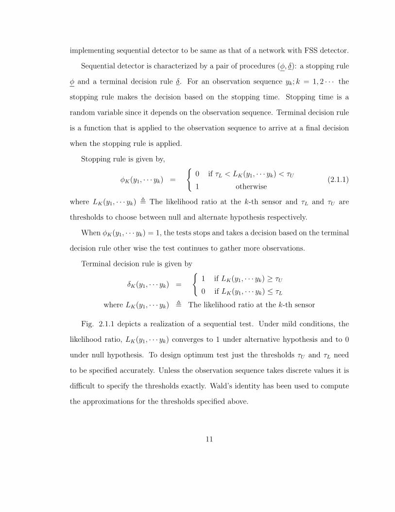
Sequential detector is characterized by a pair of procedures (φ, δ): a stopping rule

φ and a terminal decision rule δ. For an observation sequence yk; k = 1, 2 · · · the

stopping rule makes the decision based on the stopping time. Stopping time is a

random variable since it depends on the observation sequence. Terminal decision rule

is a function that is applied to the observation sequence to arrive at a final decision

when the stopping rule is applied.

Stopping rule is given by,

φK(y1, · · · yk) =

{

0 if τL < LK(y1, · · · yk) < τU

1 otherwise(2.1.1)

where LK(y1, · · · yk) , The likelihood ratio at the k-th sensor and τL and τU are

thresholds to choose between null and alternate hypothesis respectively.

When φK(y1, · · · yk) = 1, the tests stops and takes a decision based on the terminal

decision rule other wise the test continues to gather more observations.

Terminal decision rule is given by

δK(y1, · · · yk) =

{

1 if LK(y1, · · · yk) ≥ τU

0 if LK(y1, · · · yk) ≤ τL

where LK(y1, · · · yk) , The likelihood ratio at the k-th sensor

Fig. 2.1.1 depicts a realization of a sequential test. Under mild conditions, the

likelihood ratio, LK(y1, · · · yk) converges to 1 under alternative hypothesis and to 0

under null hypothesis. To design optimum test just the thresholds τU and τL need

to be specified accurately. Unless the observation sequence takes discrete values it is

difficult to specify the thresholds exactly. Wald’s identity has been used to compute

the approximations for the thresholds specified above.

11

Figure 2.1: A Realization of Sequential Test

2.2 Wald’s Identity

Wald’s identity has been a powerful tool in computing expected sample size and er-

ror probability performance of sequential tests in case of independent and identically

distributed observations [39]. The primary application of Wald’s identity is in the

sequential test analysis. It can also be applied to some sub-optimal sequential tests

and some other applications like providing Chernoff bound in the analysis of sequen-

tial algorithms for decoding trellis codes. Among all the sequential tests with the

specified error probabilities sequential probability ratio test is considered to be the

most efficient since it jointly minimizes the expected sample size for the statistical

hypotheses.

12

By applying Wald’s approximations [39], the thresholds in the equations 2.1.1 can

be given by,

τU∼=

Pd

Pf

τL∼=

1 − Pd

1 − Pf

where Pd is the probability of detection

and Pf is the probability of false-alarm

2.3 Different Sequential Testing Scenarios

As stated previously, sequential testing may be implemented in several ways based

on the system design. For instance, design in which sequential testing is implemented

at fusion or the one in which sequential testing is implemented at sensor level. Some

of the scenarios possible are briefly reviewed in this section.

2.3.1 Distributed Detection with Fusion Center Performing

the Sequential Tests

In this scenario, all the sensor nodes in the distributed architecture communicate their

local decisions or intermediate observations to the fusion center where a sequential

test is performed based on the information received from the sensors [30, 40–42] .

It can be viewed as a network analogous to a parallel network with N sensors and

the observations are independent at each sensor and from sensor to sensor. Though

the topology of the network can be compared to that of a parallel network specified

in Fig. 1.1, this detector is a variable sample-size detector as opposed to a fixed

sample-size detector of a parallel topology. At a given time, each sensor computes

13

a summary message and broadcasts that to the fusion center and all other nodes in

the network. The summary message is a function of its observation at that time and

all the previous summary messages from the other sensors. These summary messages

are communicated to the fusion center by all the sensors in the network from time to

time. Fusion center performs a sequential test based on these intermediate decisions

and decides whether to stop taking the observations and yield a final decision or

to continue taking more observations for better decision. Again the decision at the

fusion center is based on the stopping and terminal decision rules. Even though our

discussion is based on the sensors having access to all the summary messages of all

the sensors, there are various formulations which include the summary message from

a sensor based solely on its observation [42] or based on all the previous observations

at that particular sensor [40].

2.3.2 Distributed Detection with Sensors Performing Sequen-

tial Tests

In this scenario, sensor nodes perform the sequential test themselves. There is no

involvement of fusion center in this case. This topology can be compared to that of

a serial architecture depicted in Fig. 1.2 where the final decision of the network is

yielded by the last sensor in the network. But in this case the test gets stopped as soon

as enough information is gathered to decide upon a hypothesis. Joint performance

index between the sensors is achieved by coupled computations of observations [29,43].

2.3.3 Decentralized Quickest Change Detection

Decentralized quickest change detection involves detection of a brusque change in a

system based on the change in the probability distribution of the observations and

14

communicating it to the central entity with out any delay [44] . The stopping time

t is imposed based on the assumption that the observations till time t are indepen-

dent and identically distributed (i.i.d) with a specific probability distribution and the

observations after time t are i.i.d with another distribution [45], [46].

For simplicity’s sake most of the scenarios reviewed above consider binary hy-

pothesis testing for sequential detection. The problem of M-ary hypothesis testing

has been visited in [47,48].

Among these scenarios, distributed detection with sensors performing the sequen-

tial tests for a binary hypothesis testing problem has been considered in this thesis.

15

Chapter 3

Sequential Fusion in

Energy-constrained Sensor

Networks

3.1 Introduction

In classical multi-sensor systems it is a usual assumption that the data sent by sen-

sor nodes is reliably conveyed to the fusion center. But this might not be a safe

assumption considering the density of the network and noisy channels. While error

control coding can be used to minimize data corruption it might introduce extra

computational complexity over the sensor nodes and may add up to the delay as

well. A alternative framework has been introduced in [35] where the quality of the

information sent by the sensor nodes depends upon the amount of power available at

them. It has also been shown that a network having many low-cost, low-power sensor

nodes outperforms the network composed of few high-quality, high-power nodes [49],

provided the observations are conditionally independent. We explore this concept

of sensor networks to see if we can further reduce the energy consumption of these

low-power, low-cost sensor networks.

16

3.2 System Model

A binary hypothesis testing problem for a N -node wireless sensor network performing

a sequential detection is considered. Let H0 and H1 be the null and alternate hypoth-

esis respectively. Under the two hypotheses the observation yk at the k-th sensor, for

k = 1, 2, · · ·N , is assumed to be distributed as,

H0 : yk ∼ N(

−m,σ2v

)

H1 : yk ∼ N(

+m,σ2v

)

(3.2.1)

where N (m,σ2) denotes a Gaussian distribution with mean m and variance σ2. The

local observations are considered to be independent when conditioned on the hy-

pothesis. Each sensor runs a likelihood ratio test (LRT) based on its observation

and a relayed decision statistic from the previous sensor. The stopping rule specified

previously that is to be applied based on LRT is given by,

If zk =myk

σ2v

+mrk−1

rk−1

σ2rk−1

=

> τ ′U declare H1

< τ ′L declare H0

otherwise the test continues

where zk is the decision statistic at sensor k and rk−1 is the relayed decision statistic

from sensor k-1 distributed as N (mk−1, σk−1)

and τ ′U =

1

2log τU

τ ′L =

1

2log τL

If the test has to continue, the sensor k transmits its amplified decision statistic zk

to the next sensor in the network. The amplification factor a is based on the total

17

power constraint A, the K-node sensor network is subject to [35], and is given by,

a =

√

A

K(m2 + σv2)

The observation at sensor k+1 comprises of its observation, relayed decision statis-

tic from the previous sensor and the noise which can be indicated as, azk+yk+1+nk+1.

Since the sensor 1 doesn’t have a relayed decision statistic z0 is initialized to zero in

this case. Hence its LRT is purely based on its observation and noise.

It is known that SPRT is a variable sample size detection system. The performance

of the system is compared to that of a parallel architecture which is a fixed sample

size detection system. Under Neyman-Pearson (NP) criteria we compare the sample

size of both the systems required to achieve a desired level of performance.

3.3 Simulation Results

Assuming that a SPRT system requires K out of N nodes (K ≤ N) to achieve the

desired level of performance as a parallel network we explore two different scenarios

of energy consumption in the network; one in which energy per node is fixed i.e. each

node in the SPRT network has the same energy as each node in a parallel one. The

other one in which total energy of both the networks is fixed. Although SPRT network

is a N -node network it takes only K-nodes to achieve the desired performance level.

Hence this K-node energy is distributed among N -node parallel network to see the

level of performance it can achieve with the same energy as a SPRT network.

Our performance metric is the number of nodes required to achieve a desired level

of probability of detection (Pd). We investigate the performance with fixed false-

alarm probability and fixed signal-to-noise ratio (SNR). Throughout the simulations

18

0 0.1 0.2 0.3 0.4 0.5 0.6 0.7 0.8 0.9 10

5

10

15

20

25

30

35

40

45

50

No.

of S

enso

r N

odes

Probability of detection

Pd vs K

SPRT Pf = 0.1

Parallel Pf = 0.1

SPRT Pf = 0.01

Parallel Pf = 0.01

SPRT Pf = 0.001

Parallel Pf = 0.001

SPRT Pf = 0.0001

Parallel Pf = 0.0001

A=10, Observation SNR = 1 Per−node Energy is fixed

Figure 3.1: Probability of Detection vs Number of Nodes for Different False-alarmProbabilities

the total energy available to each network is fixed at 10 dB and number of nodes in

the parallel network (N) to 50.

Figs. 3.1 and 3.2 show the probability of detection achieved by the network as a

function of number of sensor nodes for different false-alarm probabilities. SNR of the

observation is fixed at 10 dB in this case. It can be observed that the average number

of nodes required to achieve the same level of performance is much less compared

to that of a parallel network. And this behavior is consistent with the increasing

false-alarm probability.

It is also expected that if more room is given for false-alarm probability i.e. if

the false-alarm increases, the number of nodes in the network can achieve greater

performance measure (Pd).

Number of nodes as a function of probability of detection for different SNRs is

19

0 5 10 15 20 25 30 35 40 45 500

0.1

0.2

0.3

0.4

0.5

0.6

0.7

0.8

0.9

1

No. of Sensor Nodes

Pro

babi

lity

of d

etec

tion

K vs Pd

SPRT Pf=0.0001

Parallel PF=0.0001

SPRT Pf=0.001

Parallel Pf=0.001

SPRT Pf=0.01

Parallel Pf=0.01

SPRT Pf=0.1

Parallel Pf=0.1

A=10, Observation SNR = 1 Per−node Energy is fixed

Figure 3.2: Number of Nodes vs Probability of Detection for Different False-alarmProbabilities

0 5 10 15 20 25 30 35 40 45 500

0.1

0.2

0.3

0.4

0.5

0.6

0.7

0.8

0.9

1

No. of Sensor Nodes

Pro

babi

lity

of d

etec

tion

K vs Pd

SPRT Obs.SNR=4Parallel Obs.SNR=4SPRT Obs.SNR=1Parallel Obs.SNR=1SPRT Obs.SNR=1/4Parallel Obs.SNR=1/4

A=10, P

f = 0.0001

Per−node Energy is fixed

Figure 3.3: Number of Nodes vs Probability of Detection for Different SNRs

20

0 0.1 0.2 0.3 0.4 0.5 0.6 0.7 0.8 0.9 10

5

10

15

20

25

30

35

40

45

50

No.

of S

enso

r N

odes

Probability of detection

K vs Pd

SPRT SNR = 1Parallel SNR = 1SPRT SNR = 1/4Parallel SNR = 1/4SPRT SNR = 4Parallel SNR = 4

A=10, P

f = 0.0001

Per−node Energy is fixed

Figure 3.4: Probability of Detection vs Number of Nodes for Different SNRs

shown in Figs. 3.3 and 3.4. The probability of false-alarm is fixed to 10−4 in this case.

It can be observed that for different SNRs the number of nodes required, to achieve

the same probability of detection as a parallel network, is less for a SPRT network.

It can also be observed that given a SPRT network, as the SNR increases the quality

of the observations also increase and hence a better probability of detection can be

achieved by the network.

Further we explore the performance achieved by the two networks by fixing the

total energy utilized by the effective number of nodes in the network. Performance

metric in this case is probability of detection as a function of number of nodes in the

network for fixed false-alarm probability. It can be observed from the figure that a

higher level of performance can be achieved by the SPRT network having the same

number of nodes as a parallel one.

21

10−2

10−1

2

3

4

5

6

7

8

9

Probability of detection

No.

of S

enso

r Nod

es

Pd vs K

SPRT Pf=0.0001

Parallel Pf=0.0001

SPRT Pf=0.001

Parallel Pf=0.001

SPRT Pf=0.01

Parallel Pf=0.01

A=10 Observation SNR=1 Total Energy Fixed Nodes In Parallel NW=50

Figure 3.5: Probability of Detection vs Number of Nodes for Fixed Total Energy forDifferent False-alarm probabilities

22

Chapter 4

Distributed Detection in Energy

and Bandwidth Constrained

Sensor Networks

4.1 Introduction

We consider dense low-power wireless sensor networks that are energy and bandwidth

constrained for distributed detection and data fusion. Current literature in distributed

detection and data fusion assumes orthogonal communication of sensors. Due to very

large number of sensors in the network, multiple sensors may have to transmit data

to the fusion center at the same time. In the case of orthogonal communication, sen-

sors need to wait for a long-time in an ”active mode” as in the case of time division

multiple access (TDMA) scheme. Moreover, total available bandwidth may be lim-

ited in orthogonal communication. This arouse the need to consider non-orthogonal

communication so that sensors can simultaneously access the channel at the same

time and go to sleep mode after transmission. So we consider Direct-sequence code-

division multiple-access (DS-CDMA) channel for sensor communication and propose

an optimal Bayesian detector for such a DS-CDMA based distributed wireless sensor

23

network having a parallel architecture in the presence of additive white gaussian noise

(AWGN). Figure 4.1 shows the proposed optimal detector for a DS-CDMA channel.

y = RA b + n

( i ) b 1

z

z 2 (i)

z 1 (i)

Final Decision

( i ) b 2

( i ) ( i ) ( i )

Sensor 2

L(z 2 (i))

Sensor 1

L(z 1 (i))

L( y (i))

Fusion Center

Detection + Fusion

L( y (i))

Figure 4.1: Optimal Bayesian Data Fusion Receiver

4.2 System Model

A binary hypothesis testing problem in a K-node wireless sensor network connected

to a data fusion center in a distributed parallel architecture [24] is considered. Let

H0 and H1 be the null and alternative hypotheses, respectively having corresponding

prior probabilities P (H0) = p0 and P (H1) = p1. Under the two hypotheses, the k-th

sensor observation zk, for k = 1, · · ·K, is assumed to be distributed as,

H0 : zk ∼ N(

0, σ2k

)

H1 : zk ∼ N(

µk, σ2k

)

(4.2.1)

where N (µ, σ2) denotes a Gaussian distribution with mean µ and variance σ2. The

local observations are considered to be independent of each other when conditioned on

24

the hypothesis. Each local sensor processes its observations independently to generate

a local decision uk ∈ {0, 1}. We assume identical likelihood ratio tests and decision

rules at all the sensors. Assuming a Bayesian approach, the decision uk of the k-th

sensor is computed as

uk =

1 ≥

if L (zk) τk

0 <

where L(zk) is the local likelihood ratio (llr) defined by

L (zk) =p(zk|H1)

p(zk|H0),

and τk is the threshold of the likelihood ratio test at the k-th sensor. Under the

Bayesian formulation, these sensor thresholds depend on the prior probabilities and

an assumed cost function [38]. Assuming independent local sensor decisions

τk =p0(C10 − C00)

p1(C01 − C11)

where Cij is the cost incurred by choosing hypothesis Hi when hypothesis Hj is true.

For the minimum probability of error detection at the local sensors, the cost function

can be chosen to be uniform:

Cij =

{

1 if i 6= j

0 if i = j

These local decisions uk’s, for k = 1, · · · , K, are next transmitted to the fusion

center over a multiple-access channel using DS-CDMA in which sensor k employs a

normalized signature waveform sk(t) of unit energy. It is assumed that local sensors

take a series of observations zk(i) corresponding to a series of true hypothesis denoted

by either H0(i) or H1(i). For simplicity, a binary phase shift keying (BPSK) system

25

is assumed, where the binary local decisions uk(i)’s, for k = 1, · · ·K, are first symbol

mapped to bk(i) ∈ {+1,−1} and then the resultant symbol stream of each sensor

k is modulated using the signature waveform sk(t) of that sensor. It is clear that

by sending the binary local decisions uk’s instead of the local observations zk’s, the

distributed detection and fusion system can reduce the transmission requirements

leading to considerable energy savings in a wireless sensor network.

Assuming symbol synchronism among the distributed sensors and an AWGN chan-

nel, the received signal at the data fusion center can be written as

r(t) =M−1∑

i=0

K∑

k=1

Akbk(i)sk(t − iT ) + n(t)

where M is the number of data symbols per sensor per frame, T is the symbol interval,

Ak is the received amplitude of sensor k, n(t) is the zero-mean AWGN receiver noise

with variance σ2 = N0

2and {sk(t); 0 ≤ t ≤ T} denotes the normalized signature

waveform of the k-th sensor.

4.3 Optimal Fusion Receiver for a DS-CDMA Wire-

less Sensor Network

Due to the assumed symbol synchronism, the Bayesian fusion problem can be for-

mulated as one of deciding between H0(i) and H1(i) based on the observed receiver

waveform {r(t) : t ∈ [iT, (i+1)T ]} in order to minimize a cost function. It can easily

be shown that a sufficient statistic for this fusion problem is given by the output of

a bank of K-matched filters each matched to a particular user signature waveform

sk(t) similar to in optimal multi-user detection. The vector of matched filter outputs

y = [y1, · · · yK ]T can then be shown to be given by [50],

y = RAb + n (4.3.1)

26

where R is the K × K normalized cross-correlation matrix of sensor signature wave-

forms, A = diag(A1 · · ·AK) is a diagonal matrix consisting of received sensor signal

amplitudes and n ∼ N (0, σ2R) is the K-vector of Gaussian receiver noise with mean

0 and covariance matrix σ2R. Note that in (4.3.1) we have dropped the time index i

since it is irrelevant due to the assumed symbol synchronism among the sensors.

The data fusion problem for the DS-CDMA wireless sensor network may be in-

terpreted as a binary-hypothesis testing based on the observation vector y. Thus, it

can be shown that the Bayesian optimal fusion rule is given by a likelihood ratio-test

(LRT) as below:

L(y) =p(y|H1)

p(y|H0)

H1

≷H0

τF

where τF is the threshold at the fusion center which depends on the prior probabilities

p0 and p1 and the cost function. In the case of minimum probability of error fusion

(uniform cost assignment) and equal a priori probabilities for two hypotheses, the

threshold for the likelihood ratio fusion becomes τF = 1.

Using the received signal model (4.3.1) the required likelihood ratio at the fusion

center can be expressed as,

L(y) =

∑

b∈{+1,−1}K p(y | b, H1) p(b | H1)∑

b∈{+1,−1}K p(y | b, H0) p(b | H0)

=

∑

b∈{+1,−1}K ebT Ay− 1

2bT ARAb p(b | H1)

∑

b∈{+1,−1}K ebT Ay− 1

2bT ARAb p(b | H0)

.

(4.3.2)

where the summations are over all possible 2K transmit symbol vectors.

Assuming that the local sensor decisions are independent we can compute the

27

conditional probabilities p(b | Hi), for i = 0, 1 as,

p(b | Hi) =K∏

k=1

p(bk | Hi)

where

p(bk | H1) =

{

1 − PMkif bk = +1

PMkif bk = 0

and

p(bk | H0) =

{

PFkif bk = +1

1 − PFkif bk = 0

with PFkand PMk

representing the false-alarm and miss probabilities of the k-th

sensor, respectively. It is assumed that fusion center knows these false-alarm and miss

probabilities associated with all sensors. Based on the local observation statistics in

(4.2.1) we may show that these local probabilities are given by

PFk= Q

(

τ ′k

σk

)

(4.3.3)

and

PMk= 1 −Q

(

τ ′k − µk

σk

)

(4.3.4)

where Q(x) denotes the Gaussian tail distribution (or Q-function) and the thresholds

τ ′k are given by,

τ ′k =

σ2k

µk

log(τk) +µk

2.

Then the optimal fusion receiver decisions are given by

δopt(y) =

1 ≥

if L (y) τF

0 <

28

where L(y) is given in (4.3.2).

As can be observed from (4.3.2), the computation of the optimal fusion rule can

be very high in complexity. For example, for the binary problem at hand, if we define

the required number of multiplications (NoM) as the time complexity of a receiver,

then the complexity of the optimal fusion scheme can be seen to be of the order of

(K + 2)2K , which is exponential in the number of users K.

4.4 Low-complexity, Partitioned Fusion Receivers

As noted above the optimal fusion receiver has a very high time complexity which is

exponential in the number of users. In order to reduce this complexity, a class of sub-

optimal fusion receivers which separate the multi-sensor detection and fusion into two

stages as shown in Fig. 4.2 are proposed. In these partitioned receivers, the multi-

sensor detection is performed at the first stage as in a traditional multiuser detector

in order to estimate the symbols bk’s transmitted by the local sensors. The estimated

symbol vector b̂ is the input to the second stage of the receiver that performs data

fusion. Next, the second stage of the receiver performs data fusion based on these

outputs as if they were the true local decisions. These partitioned receivers can be

designed so that they provide performance very close to that of the optimal fusion

receiver proposed but at a very low computational complexity.

Several well-known mulituser detectors are considered for the first stage of the par-

titioned receivers like Joint maximum likelihood (JML) detector, conventional single

user matched filter and two linear multiuser detectors namely decorrelator and mini-

mum mean square error detectors.

29

y = RA b + n

( i ) b 1

z

z 2 (i)

z 1 (i)

Final Decision

( i ) b 2

( i ) ( i ) ( i )

Sensor 2

L(z 2 (i))

Sensor 1

L(z 1 (i))

Multi -user Detector

Detection

b(i) ^ Fusion

L( b (i)) ^

Figure 4.2: Low Complexity Partitioned Receiver Model

4.4.1 Joint ML First Stage Based Partitioned Fusion Re-

ceiver

The joint ML multi-sensor detector at the first stage estimates the symbol vector b

by an estimate that maximizes the joint likelihood function of b. While JML does

not necessarily results in minimum probability of error for individual sensors it has

been shown that its performance very close to that of the minimum probability of

error detector for individual users [50]. The advantage of JML is that it is easier to

analyze than the minimum probability of error detector.

The output of the joint maximum likelihood (JML) multi-sensor detector is given

by [50]

b̂(JML)

= arg maxb∈{−1,+1}K

(2yTb − bTARAb). (4.4.1)

Next, the second stage of the partitioned receiver performs data fusion assuming

that the estimated values b̂(JML)

to be the true independent local decisions. It should

be observed that first stage decisions are not independent and the above assumption

is made to reduce the complexity at the second stage since our goal is to design

good low-complexity receivers compared to that of optimal fusion receiver. Thus, the

30

likelihood ratio employed at the second stage of the receiver is,

L(

b̂(JML)

)

=p(

b̂(JML)

| H1

)

p(

b̂(JML)

| H0

)

=K∏

k=1

p(

b̂(JML)k | H1

)

p(

b̂(JML)k | H0

) , (4.4.2)

where (due to the assumption that the first stage decisions are correct),

p(b̂(JML)k | H1) =

{

1 − PMkif b̂

(JML)k = +1

PMkif b̂

(JML)k = −1

,

and

p(b̂(JML)k | H0) =

{

PFkif b̂

(JML)k = +1

1 − PFkif b̂

(JML)k = −1

.

The required false-alarm and miss probabilities are computed as in (4.3.3) and (4.3.4).

Assuming minimum probability of error Bayesian fusion with uniform costs and equal

priors, the LRT at the fusion center is then given by,

δJML

(

b̂(JML)

)

=

1 ≥

if L(

b̂(JML)

)

1

0 <

(4.4.3)

Due to the exponential time complexity of the JML multiuser detection at the first

stage of the partitioned receiver, the time complexity for JML detector can be shown

to be of the order of K2K . Since this is not a significant improvement over the

optimal fusion receiver we look to replace the first stage with low-complexity multi-

sensor detectors.

31

4.4.2 Conventional Detector Based Partitioned Fusion Re-

ceiver

One of the simplest detectors for the multiple-access channel is the single-user matched

filter otherwise called conventional detector which, in the case of BPSK, directly quan-

tizes each component of the matched filter bank output y. Thus the output of the

single-user matched filter first stage is given by,

b̂(MF )

= sgn(y). (4.4.4)

The second stage of the receiver is exactly the same as that described above in

Section 4.4.1. i.e. the estimated bits b̂(MF )

are used to compute the likelihood ratio as

in (4.4.2) and the global decision is declared using (4.4.3). From (4.4.4) it can be seen

that time complexity for a conventional matched filter detector is greatly reduced. It

does not require any multiplications (note that likelihood-ratio computation in (4.4.2)

can be implemented as a table look-up operation).

It is known that in the presence of severe multiple-access interference the per-

formance of conventional detector can be very poor compared to the best possible

performance (however, as we will see in simulation results below in a distributed

detection based data fusion problem this may not always be true). Since linear mul-

tiuser detectors can provide a balance between performance and complexity, in the

following section two partitioned fusion receivers are considered in which the first

stage is a linear multi-sensor detector.

32

4.4.3 Linear Multi-sensor Detector First Stage Based Fusion

receivers

The first linear detector we used is the decorrelator:

b̂(decor)

= sgn(R−1y)

The decorrelator zero-forces the multiple-access interference for each user at the ex-

pense of noise enhancement. In order to minimize the combination of interference

and noise we may instead use the minimum mean square error (MMSE) multi-sensor

detector:

b̂(MMSE)

= sgn((R + σ2A−2)−1y)

In terms of number of required multiplications both these detectors has a time com-

plexity of K (note that matrix inverses can be pre-computed since they are fixed for

the synchronous channel). The fusion rule at the second stage is again exactly the

same as that in (4.4.2) and (4.4.3).

4.4.4 Simulation Results Optimal Fusion and Partitioned De-

tectors

The performance and complexity trade-offs of the optimal fusion receiver and the

partitioned low-complexity receivers are investigated via several representative nu-

merical examples. Although in all cases we limit ourselves to a binary hypothesis

testing problem and a BPSK-based synchronous DS-CDMA communications over

an AWGN channel, this model can be safely extended to fading channels [51]. The

Bayesian cost function considered is the minimum probability of error with equally

probable hypotheses. Thus, the performance metric is the probability of error at

33

the output of the fusion receiver. Considering a 4-node architecture the value of

cross-correlation coefficient is set at 0.7 for all the results shown. The performance

of different detectors as a function of signal-to-noise (SNR) is investigated . Fig. 4.3

shows the performance of the fusion receivers as a function of average local SNR for

fixed channel SNR value of 6 dB for all k.

−2 0 2 4 6 8 10 1210

−3

10−2

10−1

100

Local Sensor SNR in dB

Fu

sio

n P

e

Fusion Pe vs. Local Sensor SNR for DS−CDMA in AWGN

K = 4, rho = 0.7, Channel SNR = 6dB

conv. detector based fusionJML detector based fusionDecorrelator based fusionMMSE based fusionOptimal fusionsensor 1 local decisions

Figure 4.3: Fusion Probability of Error vs Average Local SNR for Fixed ChannelSNR = 6dB for all k

It is evident from Fig. 4.3, the performance of JML and conventional detector based

partitioned receivers are very close to that of optimal fusion receiver. It can also

be observed that the performance of decorrelator based partitioned receiver is poor

among all the fusion receivers and its performance is similar to that of individual

34

sensor’s probability of error. Although it is surprising that the performance of con-

ventional detector based partitioned receiver is close to that of optimal fusion receiver

in AWGN channel, its performance degrades severely in Rayleigh fading channel [51].

−4 −2 0 2 4 6 8 10 12 1410

−3

10−2

10−1

100

Channel SNR in dB

Fu

sio

n P

e

Fusion Pe vs.Channel SNR for DS−CDMA

K = 4, rho = 0.7, Local SNR = 10 dB

conv. detector based fusionJML detector based fusionDecorrelatorOptimal fusionsensor 1 local decisions

Figure 4.4: Fusion Probability of Error vs Average Channel SNR for Fixed LocalSNR = 10dB for all k

Fig. 4.4 shows the fusion probability of error performance as a function of the average

channel SNR for a fixed local sensor SNR value for all k sensor nodes at 10dB. It can

be observed from the figure that the performance of the receivers at the fusion center

are highly dependent on the local sensor SNR i.e. even though the channel SNR

improves, the fixed local SNR value limits the performance of the fusion receivers

and the performance of partitioned receivers converge to that of the optimal fusion

35

receiver. Moreover, it can also be observed that there is a clear channel SNR below

which single sensor performance is better than that of fusion receivers.

36

Chapter 5

Conclusions

The main focus of this thesis work is to explore various distributed detection and data

fusion strategies for energy and bandwidth constrained sensor networks. In the case

of networks which are energy-constrained SPRT based energy-efficient distributed

detection model has been proposed. From the numerical results it can be concluded

that the proposed network model achieves higher level of performance when compared

to that of fixed sample-size detector based networks. With fixed per-node energy the

proposed SPRT based detection model results in very less number of nodes required to

achieve the probability of detection compared to that of parallel architecture network.

With fixed total-energy in the network, the probability of detection achieved by a

SPRT based network is improved when compared to a parallel network having same

number of nodes.

In the case of energy and bandwidth constrained sensor networks optimal Bayesian

fusion receiver operating in non-orthogonal communication channel (DS-CDMA) is

proposed and it can observed that its complexity is exponential in the number of

local sensor nodes. In order to reduce this complexity, a class of sub-optimal fusion

receivers are proposed by partitioning the multi-sensor detection and data fusion

37

into two consecutive stages. For the first stage multi-sensor detection several well

known multiuser detectors such as joint maximum likelihood, conventional single-user

matched filter, decorrelator and minimum mean square error detector are investigated.

In the case of JML first stage based receiver which was found to perform very close to

the optimal fusion receiver in most cases has an exponential complexity. However, the

single-user matched filter first stage based fusion receiver also performs remarkably

well, and in particular close to the performance of optimal receiver, as long as there

is not a large power imbalance in the channel SNR values. Moreover, while fusion

performance is not limited by a fixed channel SNR value when the local SNR values

are increasing, for a fixed local SNR value we observed that the performance will

be limited by it for large channel SNR values. In this case, the performance of all

partitioned receivers approaches that of the optimal fusion receiver for large channel

SNR values.

As a possible extension for future work, the data dependency in the case of energy-

constrained sensor networks based on SPRT based detection model can be explored.

38

BIBLIOGRAPHY

39

[1] K. Sohrabi, J. Gao, V. Ailawadhi, and G. J. Pottie, “Protocols for self- organization of a

wireless sensor network,” IEEE. Pers. Comm., vol. 7, no. 5, pp. 16–27, Oct. 2000.

[2] J. Kahn, R. Katz, and K. Pister, “Next century challenges: Mobile networking for

‘smart dust’,” Proc. MOBICOM, 1999.

[3] L. Schwiebert, S. K. S. Gupta, and J.Weinmann, “Research challenges in wireless

networks of biomedical sensors,” Seventh Annual Intl. Conf. on Mobile Comp.and

networking, pp. 151–165, 2001.

[4] A. Cerpa, J. Elson, D. Estrin, L. Girod, M. Hamilton, and J. Zhao, “Habitat mon-

itoring: Application driver for wireless communications technology,” Proc. of Ist ACM

SIGCOMM Workshop on Data Comm. in Latin America and Caribbean, 2001.

[5] M. I. Selventoinen and T. Rantalainen, “Mobile station emergency locating in GSM,”

IEEE Intl. Conf. on Personal Wireless Communications, 1996.

[6] I. F. Akyildiz, W. Su, Y. Sankarasubramaniam, and E. Cayirci, “A survey on sensor

networks,” IEEE Comm. Magazine, Aug. 2002.

[7] W. B. Heinzelman, “Application-specific protocol architectures for wireless net-

works,” Ph.D. dissertation, Massachusetts Institute of Technology, 2000.

[8] A.Woo and D. E. Culler, “A transmission control scheme for media access in sensor

networks,” Seventh Annual Intl conf. on Mobile computing and networking, Jul. 2001.

[9] M. Dong, K. Yung, and W. Kaiser, “Low-power signal processing architectures for

network micro-sensors,” in Proc. of 1997 Intl. Symposium On Low Power Electronics

and Design, Aug. 1997, pp. 173–177.

40

[10] S. Patil, S. Das, and A. Nasipuri, “Serial data fusion using space-filling curves in

wireless sensor networks,” in Proc of 1st Intl. Conf On Sensor and Adhoc

Communications and Networks (SECON’04), Santa Clara, CA, USA, Oct. 2004.

[11] D. Ganesan, R. Govindan, S. Shenker, and D. Estrin, “High-resilient energy-efficient

multi-path routing in wireless sensor networks,” IEEE Infocom, 2002.

[12] V. Raghunathan, C. Schurgers, S. Park, and M. B. Srivastava, “Energy-aware wireless

microsensor networks,” IEEE Sig. Pro. Mag., pp. 40–50, Mar. 2002.

[13] R. Min, M. Bharadwaj, S. Cho, N. Ickes, E. Shih, A. Sinha, A. Wang, and A. P.

Chandrakasan, “Energy-centric enabling technologies for wireless sensor networks,”

IEEE Wireless Communications, no. 4, pp. 28–39, Aug. 2002.

[14] V. Rodoplu and T. H. Meng, “Minimum energy mobile wireless networks,” IEEE

JSAC, no. 8, pp. 28–39, Aug. 1999.

[15] L. Li and J. Y. Halpern, “Minimum energy mobile wireless networks revisited,” ICC,

Jun. 2001.

[16] A. Manjeshwar and D. P. Agrawal, “Teen : A protocol for enhanced efficiency in

wireless sensor networks,” Proceedings of the 1st International Workshop on Parallel

and Distributed Computing Issues in Wireless Networks and Mobile Computing, in

conjunction with 2001 IPDPS, Apr. 2001.

[17] W. R. Heinzelman, A. Chandrakasan, and H. Balakrishnan, “Energy efficient

communication protocol for wireless micro-sensor networks,” IEEE Proc. of

Intl.Hawaii. Conf. on Sys. Sci., pp. 1–10, Jan. 2000.

[18] A. Sinha and A. Chandrakasan, “Dynamic power management in wireless sensor

networks,” IEEE Design Test Comp., Mar/Apr. 2001.

41

[19] R. R. Tenney and N. R. S. Jr., “Detection with distributed sensors,” IEEE Trans.

Aerospace and Electronic Systems, vol. AES-17, pp. 501–510, Jul. 1981.

[20] R. S. Blum, S. A. Kassam, and H. V. Poor, “Distributed detection with multiple sensors

part ii - advanced topics,” Proc of IEEE, vol. 85-1, pp. 64–79, Jan. 1997.

[21] Z. Chair and P. K. Varshney, “Optimal data fusion in multiple sensor detection

systems,” IEEE Trans. Aerospace and Electronic Systems, vol. 22-1, pp. 98–101,1986.

[22] S. C. A. Thomopoulos, R. Viswanathan, and D. Bougoulias, “Optimal distributed

decision fusion,” IEEE Trans. Aerospace and Electronic Systems, vol. 25, pp. 761–765,

Sep. 1989.

[23] J. N. Tsistsiklis, “Decentralized detection,” Advances in Statistical Signal Processing,

Signal Detection.

[24] P. K. Varshney, Distributed Detection and Data Fusion. New York: Springer Verlag,

1996.

[25] G. Fedele, L. Izzo, and L. Paura, “Optimal and sub-optimal space-diversity detection of

weak signals in non-gaussian noise,” IEEE Trans. Commun., vol. COM-32, pp. 990–

997, Sept. 1984.

[26] R. Srinivasan, “The detection of weak signals using distributed sensors,” 24th Annual

Intl conf. on Informat. Sci. and Sys., Mar. 1990.

[27] Z. B. Tang, K. Pattipati, and D. L. Kleinman, “Optimization of detection networks: Part

1-tandem structures,” IEEE Trans. Syst. Man Cybern., vol. 21, pp.1044–1059, Sept.

1991.

42

[28] K. P. Z. B. Tang and D. L. Kleinman, “Optimization of distributed detection networks:

Part ii generalized tree structures,” IEEE Trans. Syst. Man Cybern., vol. 23, pp. 211–

221, Jan/Feb. 1993.

[29] V. V. Veeravalli, T. Basar, and H. V. Poor, “Decentralized sequential detection with

sensors performing sequential tests,” Journal on Math. of Contrl. Signals and Systems,

vol. 7-4, pp. 292–305, Dec. 1994.

[30] ——, “Decentralized sequential detection with a fusion center performing the

sequential test,” IEEE. Trans. on. Inform. Theory, vol. 39-2, pp. 433–442, Mar. 1993.

[31] S. Kassam and J. Thomas, Nonparametric detection - theory and applications. Dowden,

Hutchinson and Ross, 1980.

[32] M. Hollander and D. A. Wolfe, Nonparametric statistical methods (2nd Edition).

Wiley, New York, 1991.

[33] Y. Q. Yin and P. R. Krishnaiah, “On some nonparametric methods for detection of the

number of signals,” IEEE Trans. Acoustics, Speech, and Signal Processing, vol. ASSP-

35, no. 11, p. 1533, 1987.

[34] S. A. Kassam and H. V. Poor, “Robust techniques for signal processing: A survey,”

Proc. IEEE, vol. 73, pp. 433–481, 1985.

[35] J. F. Chamberland and V. V. Veeravalli, “Decentralized detection in wireless sensor

systems with dependent observations,” in Proc. of 2nd Intl. Conf. On. Computing,

Commun and Control Technologies(CCCT04), Austin, TX, USA, Aug. 2004.

[36] V. V. Veeravalli, “Sequential decision fusion: Theory and applications,” in Proc of

Workshop on Foundations of Information/Decision Fusion: Applications to

Engineering Problems.

43

[37] ——, “Comments on decentralized sequential detection,” IEEE Trans. on Information.

Theory, vol. 38-4, pp. 1428–1429, Jul. 1992.

[38] H. V. Poor, Introduction to Signal Detection and Estimation, Second Edition.New

York: Springer-Verlag, 1994.

[39] A. Wald, Sequential Analysis. New York: Wiley, 1947.

[40] H. R. Hashemi and I. B. Rhodes, “Decentralized sequential detection,” IEEE. Trans. on.

Inform. Theory, vol. 35-3, pp. 509–520, May. 1989.

[41] V. V. Veeravalli, “Sequential decision fusion,” Journal of the Franklin Institute, vol.

336-2, pp. 201–322, Feb. 1999.

[42] J. N. Tsitsiklis, “On threshold rules in decentralized detection,” Proc of 25th IEEE Conf.

Decision and Contr.,, pp. 232–236, 1986.

[43] D. Teneketzis and Y. C. Ho, “The decentralized wald problem,” Inform. Comput,1987.

[44] D. Teneketzis and P. Varaiya, “The decentralized quickest detection problem,” IEEE

Trans. Automatic Contr., vol. AC-29, pp. 641–644, Jul. 1984.

[45] R. W. Crow and S. C. Schwartz, “Quickest detection for sequential decentralized

decision systems,” IEEE Trans. Aerospace and Electronic Systems, vol. 32, pp.267–

283, Jan. 1996.

[46] V. V. Veeravalli, “Decentralized quickest change detection,” IEEE. Int. Symp. Inform.

Theory., p. 294, 1995.

[47] C. W. Baum and V. V. Veeravalli, “A sequential procedure for multihypothesis

testing,” IEEE Trans. on Information. Theory, vol. 40-6, pp. 1994–2007, Nov. 1994.

[48] V. V. Veeravalli and C. W. Baum, “New results in m-ary sequential hypothesis

testing,” in Proc. 27th Annual Conference on Information Sciences and Systems.

44

[49] J. F. Chamberland and V. V. Veeravalli, “Decentralized detection in sensor networks,”

IEEE. Trans. Signal. Processing, vol. 51-2, pp. 407–416, Feb. 2003.

[50] S. Verdu, Multiuser Detection. New York: Springer-Verlag, 1994.

[51] S. K. Jayaweera, “Optimal bayesian data fusion and low complexity approximations for

distributed ds-cdma wireless sensor networks in rayleigh fading,” in 2nd Int. Conf. on

Intelligent Sensing and Information Processing (ICISIP 05), Chennai, India, Jan. 2005.

45