distortions in resource allocation and bank lending
TRANSCRIPT

No.07-E-6 March 2007
DistortBank Financi
Akira Otaniakira.ootani@b
Shigenori Sshigenori.shira
Takeshi Yatakeshi.yamad
Bank of Japan 2-1-1 Nihonbas
* Financial Syst** Financial Sys*** Financial Sys
Papers in the Banand comments. VBank. If you have any cWhen making a Public Relationspermission. WhSeries, should ex
ions in Resource Allocation and Lending: The Malfunction of al Intermediation
* oj.or.jp
hiratsuka ** [email protected]
mada *** [email protected]
hi Hongoku-cho, Chuo-ku, Tokyo 103-8660
ems and Bank Examination Department tems and Bank Examination Department tems and Bank Examination Department
k of Japan Working Paper Series are circulated in order to stimulate discussion iews expressed are those of authors and do not necessarily reflect those of the
omment or question on the working paper series, please contact each author. copy or reproduction of the content for commercial purposes, please contact the Department ([email protected]) at the Bank in advance to request en making a copy or reproduction, the source, Bank of Japan Working Paper
plicitly be credited.
Bank of Japan Working Paper Series

Distortions in Resource Allocation and Bank Lending: the Malfunction of Financial Intermediation
Akira Otani*, Shigenori Shiratsuka**, and Takeshi Yamada***
March 2007
Abstract
In this paper, we empirically analyze the interaction between the distortions in the real side of the economy (real distortion) and those in the financial side of the economy (financial distortion) in Japan after the 1990s. We focus on protracted economic stagnation after the bursting of the asset price bubble, and the subsequent recovery in economic activity and restoration of financial system stability. We use the intersectoral differences in relative factor prices as an indicator for the real distortion, and use the gap between the actual and benchmark loan portfolios, based on the mean-variance approach to maximize risk adjusted returns from loan portfolios, as an indicator for financial distortion. We show that both distortions sharply deteriorated in the late 1990s and improved in the 2000s. In addition, we conduct panel data analyses using data at individual bank level as well as at industry level to examine the interaction between the two distortions: the interaction was negative in the late 1990s, but reversed to positive in the 2000s. Key Words: Efficiency in Resource Allocation, Interaction between Real and Financial
Distortions, Mean-Variance Approach JEL Classification Code: G21, G28, O47
* Financial Analysis and Research, Financial Systems and Bank Examination Department, Bank
of Japan (E-mail: [email protected]) ** Financial Analysis and Research, Financial Systems and Bank Examination Department, Bank
of Japan (E-mail: [email protected]) *** Financial Analysis and Research, Financial Systems and Bank Examination Department, Bank
of Japan (E-mail: [email protected]) The authors thank Kazuhito Ikeo, Kunio Okina, Masaaki Shirakawa, and staff of the Financial Systems and Bank Examination Department, Monetary Affairs Department, Research and Statistics Department, and Institute for Monetary and Economic Studies, Bank of Japan, for their helpful comments, and Mitsuru Katagiri, Yuko Suda, and Ryoko Tsurui for their helpful assistance. The views expressed in this paper are those of the authors and do not necessarily reflect the official views of the Bank of Japan or the Financial Systems and Bank Examination Department.
Table of Contents
I. Introduction ................................................................................................................ 1
II. Distortions in Resource Allocation in the Real Side of the Economy...................... 3
A. Distortions in Intersectoral Resource Allocation................................................ 4
B. Decomposition of GDP Growth Rate with Distortions in Resource Allocation 6
III. Distortions in the Financial Side of the Economy................................................... 8
A. Distortions in Bank Loan Portfolios................................................................... 8
B. Results of Estimating Distortions in Bank Loan Portfolios ............................. 10
C. Distortions in Bank Loan Portfolios and Functioning of Bank’s Financial
Intermediation............................................................................................................. 12
IV. Relation between Distortions in Resource Allocation and Distortions in Bank
Loan Portfolios ........................................................................................................... 14
A. Effect of Real Distortions on Financial Distortions .............................................. 14
B. Effect of Financial Distortions on Real Distortions............................................... 16
C. Summary of Empirical Results .............................................................................. 18
V. Concluding Remarks .............................................................................................. 18
References ...................................................................................................................... 21

1
I. Introduction
A number of theoretical and empirical studies have examined the causes of Japan’s
protracted economic stagnation after the 1990s.1
Focusing on the real economic factors, Hayashi and Prescott (2002) decompose
GDP growth rate, assuming complete factor markets, and show that declines in work
hours and TFP (total factor productivity) growth induced Japan’s long-lasting
stagnation in the 1990s.2 Nakakuki, Otani, and Shiratsuka (2004) and Miyagawa (2006)
point out that misallocations of productive resources due to incomplete factor markets
led to the long-lasting poor economic performance during the period of Japan’s
protracted economic stagnation after the 1990s.
Focusing alternatively on the financial factors, Hoshi and Kashyap (1999) show
that the malfunction of financial intermediation was caused by the non-performing loan
problem after the bursting of the asset price bubble against the background of financial
deregulations: on the one hand, large firms shifted from bank borrowing to
capital-market financing, and, on the other hand, banks were forced to make aggressive
lending to small and medium-sized firms as well as construction and real estate
industries. Sekine, Kobayashi, and Saita (2003), Hoshi (2003), and Peek and Rosengren
(2005) show that banks with impaired capital are likely to make additional loans to
troubled firms. This empirical evidence indicates that these firms keep employing
productive resources owing to the forbearance loan and thus this behavior of banks
could exert a negative effect on economic activity.
As for the relation between economic factors and financial factors, Nagahata and
1 Structural problems are pointed out as one of the major factors behind the long lasting economic stagnation. Maeda, Higo, and Nishizaki (2001) categorize causes of structural impediments into four: (i) rigid corporate governance; (ii) inefficiency of the non-manufacturing sector; (iii) the issue of non-performing assets with the generation and bursting of the asset price bubble; and (iv) the savings-investment imbalance. They argue that all of these are “impediments to the efficient allocation of resources.” In this paper, we focus on inefficient resource allocations due to distortions in the real side and the financial side of the economy, rather than individual factors behind the structural problems, from macroeconomic viewpoints.
2 Kawamoto (2005) estimates the pure technological progress by adjusting industrial return on scale, labor and capital utilization, and reallocation of productive resources among industries, and shows that it did not decelerate in the 1990s.

2
Sekine (2005) demonstrate that corporate investment of small enterprises which have
not issued corporate bonds decreased drastically owing to the deterioration in the main
banks’ balance sheet conditions. Caballero, Hoshi, and Kashyap (2006) show that
industries with many zombies (insolvent firms enjoying interest concession) exhibit
more depressed job creation and low productivity growth, suggesting that an increase in
loans to zombies exerts a negative impact on the real economy.
Okina and Shiratsuka (2002) suggest the mechanism behind the interaction
between real distortions and financial distortions.3 That is, they look back at Japan’s
experiences after the bursting of the asset price bubble, and argue that significant
declines in asset prices impaired banks’ capital positions and their intertemporal risk
smoothing function. Then, they conjecture that the resultant financial instability
amplified the adverse effects of the bursting of the asset price bubble on the real side of
the economy. 4 The previous studies on Japan’s prolonged economic stagnation
mentioned above, however, analyze the real economic factors and the financial factors
separately, and do not fully explore their interaction.
In this paper, we attempt to analyze the interaction between the distortions in the
real side of the economy (real distortion as misallocations in factor markets) and those
in the financial side of the economy (financial distortion as a deviation of banks’
behavior from profit maximization, including “forbearance lending” and “credit
crunch”) during the period of Japan’s protracted economic stagnation after the 1990s
and the subsequent recovery. We construct indicators to trace each distortion and then
empirically analyze their relation.
We use the intersectoral differences in relative factor prices as an indicator for
the real distortion, employed in Nakakuki, Otani, and Shiratsuka (2004). We also use
the gap between the actual and benchmark loan portfolios, based on the mean-variance
approach to maximize risk adjusted returns from loan portfolios, as the indicator for
financial distortion. The previous literature, including Sekine, Kobayashi, and Saita
3 Saito (2006) argues that macroeconomic policy which was intended to lower the real interest rate caused excess capital accumulation in the low productivity sector in the late 1980s, resulting in a decrease in capital productivity in the 1990s.
4 See Allen and Gale (1997) as literature which theoretically shows the banks’ intertemporal risk smoothing function.
3
(2003) and Peek and Rosengren (2005), regards the provision of additional loans to
troubled firms as a distortion in bank loan portfolios. Banks, however, try to keep
troubled firms alive not only by providing additional loans, but also by rolling
outstanding loans over, and providing financial assistance such as the forms of debt
forgiveness and debt equity swaps. The indicator for the financial distortion used in this
paper grasps more comprehensive distortions in bank loan portfolios including not only
forbearance lending but also other types of financial assistance and credit crunch.5
Our empirical evidence suggests two points. First, both distortions in factor
markets and banks’ loan portfolios drastically deteriorated in the late 1990s, followed
by remarkable improvement in the 2000s. Second, the panel data analyses show that the
interaction between the two distortions produced persistent adverse effects, triggered by
the bursting of the asset price bubble in the late 1990s, but such negative interaction
reversed to positive as the financial system has stabilized in the 2000s.
This paper is structured as follows. In Section II, we explain the indicator for the
distortions in factor markets, proposed in Nakakuki, Otani, and Shiratsuka (2004), and
examine the time-series movements of the estimates. In Section III, we formulate an
indicator for the distortions in bank loan portfolios using the gap between the actual and
benchmark loan portfolios, based on the mean-variance approach to maximize risk
adjusted returns from loan portfolios. In Section IV, we conduct panel data analysis to
investigate the relation between real and financial distortions, thereby showing the
interaction between the two. In Section V, we offer a concluding discussion by
examining implications for prudential policy.
II. Distortions in Resource Allocation in the Real Side of the Economy
Nakakuki, Otani, and Shiratsuka (2004) estimate the distortions in resource allocation
using the intersectoral differences in relative factor prices, proposed by Johnson (1966)
and Jones (1971). In this section, we explain the indicator for the distortions in factor
5 Caballero, Hoshi, and Kashyap (2006) and Hoshi (2006) identify zombies by classifying firms based on the assumption of whether their paying interest rate is less than the minimum required interest rate calculated by the prime rate. This identification measure includes not only forbearance lending conducted at low rates but also debt equity swaps and debt forgiveness.

4
markets, employed in Nakakuki, Otani, and Shiratsuka (2004), and examine the
time-series movements of the estimates. The estimates suggest that the distortions in
non-manufacturing industries, including construction and wholesale and retail trade,
dramatically worsened toward the end of the 1990s and are improving in the 2000s.
Then we carry out a growth accounting exercise, incorporating the effects of
misallocation in factor markets, to show that the recent economic recovery depends
partly on the improvement in resource allocation.
A. Distortions in Intersectoral Resource Allocation
Suppose that perfect competition holds and that the production function of each sector is
homogeneous to degree one and defined by the equation below,
),( iiiii LKFAY = ,
where the subscript i denotes sector and Y, A, K, and L represent output, TFP, capital
stock, and labor input, respectively. Dividing the above equation by labor input yields
labor productivity (y = Y/L), which can be expressed by the capital-labor ratio (k = K/L)
as follows:
)( iiii kfAy = ,
where )( ii kf is )1,/( iii LKF . Since the ratio of wages (wi) to the rate of return on
capital (ri) in sector i is equal to the ratio of labor’s marginal productivity to capital’s
marginal productivity, the equation below holds:
)(')(')(
ii
iiiii
i
i
kfkkfkf
rw −
=.
(1)
The labor share in sector i ( iα ) equals )(/)('1 iiiii kfkkf− and capital share ( iα−1 )
equals )(/)(' iiiii kfkkf .6 Using them, (1) can be transformed as follows:
6 Estimating the real distortion, we assume the labor share and capital share are constant during the sample period.
5
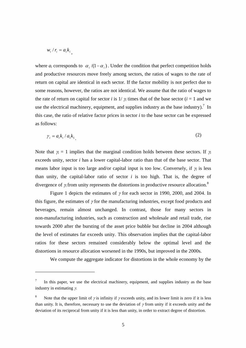
iiii karw =/ ,
where ai corresponds to )1/( ii αα − . Under the condition that perfect competition holds
and productive resources move freely among sectors, the ratios of wages to the rate of
return on capital are identical in each sector. If the factor mobility is not perfect due to
some reasons, however, the ratios are not identical. We assume that the ratio of wages to
the rate of return on capital for sector i is 1/ γi times that of the base sector (i = 1 and we
use the electrical machinery, equipment, and supplies industry as the base industry).7 In
this case, the ratio of relative factor prices in sector i to the base sector can be expressed
as follows:
11/ kaka iii =γ .
(2)
Note that γi = 1 implies that the marginal condition holds between these sectors. If γi
exceeds unity, sector i has a lower capital-labor ratio than that of the base sector. That
means labor input is too large and/or capital input is too low. Conversely, if γi is less
than unity, the capital-labor ratio of sector i is too high. That is, the degree of
divergence of γi from unity represents the distortions in productive resource allocation.8
Figure 1 depicts the estimates of γ for each sector in 1990, 2000, and 2004. In
this figure, the estimates of γ for the manufacturing industries, except food products and
beverages, remain almost unchanged. In contrast, those for many sectors in
non-manufacturing industries, such as construction and wholesale and retail trade, rise
towards 2000 after the bursting of the asset price bubble but decline in 2004 although
the level of estimates far exceeds unity. This observation implies that the capital-labor
ratios for these sectors remained considerably below the optimal level and the
distortions in resource allocation worsened in the 1990s, but improved in the 2000s.
We compute the aggregate indicator for distortions in the whole economy by the
7 In this paper, we use the electrical machinery, equipment, and supplies industry as the base industry in estimating γ.
8 Note that the upper limit of γ is infinity if γ exceeds unity, and its lower limit is zero if it is less than unity. It is, therefore, necessary to use the deviation of γ from unity if it exceeds unity and the deviation of its reciprocal from unity if it is less than unity, in order to extract degree of distortion.
6
average of γ weighted by the sector’s share of nominal GDP. The distortions worsened
in the 1990s and dramatically improved in 2001. Since 2001, they have continued to
improve gradually (see Figure 2)9.
B. Decomposition of GDP Growth Rate with Distortions in Resource Allocation
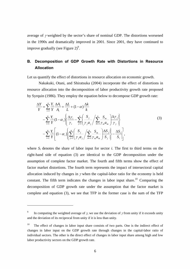
Let us quantify the effect of distortions in resource allocation on economic growth. Nakakuki, Otani, and Shiratsuka (2004) incorporate the effect of distortions in
resource allocation into the decomposition of labor productivity growth rate proposed
by Syrquin (1986). They employ the equation below to decompose GDP growth rate:
, )1(
)1(
)1(
1 1 1
1 1 1
1
∑ ∑ ∑
∑ ∑ ∑
∑
= = =
= = =
=
⎥⎥⎦
⎤
⎢⎢⎣
⎡ Δ−
⎪⎭
⎪⎬⎫
⎪⎩
⎪⎨⎧ Δ
⎟⎟⎠
⎞⎜⎜⎝
⎛−−
⎪⎭
⎪⎬⎫
⎪⎩
⎪⎨⎧ Δ
⎟⎟⎠
⎞⎜⎜⎝
⎛−
Δ−−
Δ−+
Δ+
Δ=
Δ
n
i i
in
j j
jn
m mm
m
jj
ji
i
n
i
n
j j
jn
m mm
m
jj
j
i
ii
i
n
i i
ii
SS
SS
aS
aS
YY
aS
aS
YY
kk
LL
AA
YY
YY
γγα
γγ
γγγγ
α
α
(3)
where Si denotes the share of labor input for sector i. The first to third terms on the
right-hand side of equation (3) are identical to the GDP decomposition under the
assumption of complete factor market. The fourth and fifth terms show the effect of
factor market distortions. The fourth term represents the impact of intersectoral capital
allocation induced by changes in γ when the capital-labor ratio for the economy is held
constant. The fifth term indicates the changes in labor input share.10 Comparing the
decomposition of GDP growth rate under the assumption that the factor market is
complete and equation (3), we see that TFP in the former case is the sum of the TFP
9 In computing the weighted average of γ, we use the deviation of γ from unity if it exceeds unity and the deviation of its reciprocal from unity if it is less than unity.
10 The effect of changes in labor input share consists of two parts. One is the indirect effect of changes in labor input on the GDP growth rate through changes in the capital-labor ratio of individual sectors. The other is the direct effect of changes in labor input share among high and low labor productivity sectors on the GDP growth rate.

7
growth rate and the effect of factor market distortions in equation (3). This indicates that
the TFP growth rate estimated under the assumption of complete factor market is not
the “true” TFP growth rate, because this assumption ignores the negative effect of factor
market distortions.
Table 1 shows the results of decomposing Japan’s GDP growth rate based on
equation (3).11,12 In the 1990s after the bursting of the bubble (1992–2000), the GDP
growth rate decelerates, since the positive contributions of both accumulation in capital
and TFP declined and the contribution of labor input turns negative. Moreover, the
effect of intersectoral differentials in factors’ marginal productivity turns negative.13
In the 2000s (2001–2004), the negative contribution of labor input expands, and
the positive contribution of capital accumulation declines. Moreover, the positive
contribution of changes in labor input share declines due to a shift of labor input to low
productivity sectors, including the service industry. The positive contribution of TFP,
however, increases and moreover the contribution of intersectoral differentials in
factors’ marginal productivity dramatically improves. This suggests that improvements
11 The following data are used in breaking down the GDP growth rate. Y: real GDP, L: product of workers and their average work hours, α: nominal employee compensation divided by nominal domestic factor income, and K: product of real capital stock and capacity utilization. The source for Y, L, and α is the Cabinet Office, National Account. The source for K is the JIP database. For details of the JIP database, see Fukao et al. (2003). Note that because data for capital stock and capacity utilization is released only up to 1998 in the JIP database, we use data in the Annual Report on Gross Capital Stock of Private Enterprises as those for capital stock since 1999 and estimate the data for capital utilization since 1999 using capital utilization in the Industrial Production Index for manufacturing industries and electric power consumption for non-manufacturing industries.
12 In breaking down the GDP growth rate, the qualities of labor input are assumed to be identical among every sector. It follows that labor reallocation from low labor productivity sectors to high productivity sectors results in increased labor productivity for the economy. In reality, however, the quality of labor input and expertise necessary for production activity varies among firms and sectors. Thus, the shift of labor allocation to sectors that require different expertise could lead to wasted human capital and a decrease in labor productivity. Some cautions are thus in order in interpreting the empirical results.
13 On the face of it, the negative contribution of factor market distortions may look small, compared with other factors. It should be noted, however, that the above result shows the estimate of the direct impacts of factor market distortions, so it ignores the indirect impacts, including deceleration in capital accumulation due to factor market distortions.

8
in productive resource allocation push up GDP growth rate, thereby strengthening the
momentum toward sustainable growth.
III. Distortions in the Financial Side of the Economy
In this section, we propose a framework to quantitatively evaluate distortions in loan
portfolios as distortions in resource allocation in the financial side of the economy. We
calculate the hypothetical loan portfolios based on the mean-variance approach to
maximize risk adjusted returns from loan portfolios as a benchmark and then estimate
the gap between actual and benchmark loan portfolios.14
Many previous studies employ the criterion of distortions in bank loan portfolios
to judge whether additional loans are to be provided to troubled firms just to avoid
bankruptcy. To keep insolvent firms alive, banks not only provide additional loans
(forbearance lending), but also maintain their loans, or even provide financial assistance
in the form of debt forgiveness and/or debt equity swaps to firms whose loans should be
called in from the standpoint of risk adjusted return. Moreover, banks do not provide
sufficient funds to growing firms (credit crunch), since an increase in non-performing
loans impairs banks’ capital and thus deteriorates their risk-taking ability. It is thus
deemed effective to use the gap between actual loan portfolios and benchmark ones,
instead of additional loans, in order to grasp the comprehensive distortions in bank loan
portfolios.
A. Distortions in Bank Loan Portfolios
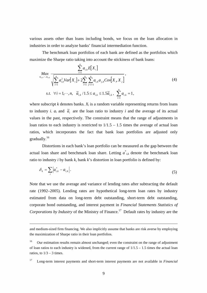
We define the benchmark bank loan portfolio as one that maximizes the Sharpe ratio, i.e.
return divided by risk, in the total loan portfolios (see Figure 3).15 Although banks hold
14 The mean-variance approach is widely used in estimating banks’ benchmark asset portfolios. For example, Buch, Driscoll, and Ostergaard (2004) estimate the gaps between actual banks’ portfolios in international investment and benchmark portfolios that maximize risk adjusted return. They then show that the gaps between actual and benchmark portfolios are attributable to information asymmetry between home and foreign countries and capital controls.
15 Note that we implicitly assume that banks are price-takers and are exogenously given the size of their loan portfolios. The benchmark loan portfolios estimated by the mean-variance approach in this paper are not necessarily equal to “true” optimal portfolios, considering banks’ specialty in small
9
various assets other than loans including bonds, we focus on the loan allocation in
industries in order to analyze banks’ financial intermediation function.
The benchmark loan portfolios of each bank are defined as the portfolios which
maximize the Sharpe ratio taking into account the stickiness of bank loans:
[ ]
[ ] [ ]∑ ∑ ∑
∑
= = +=
=
⋅⋅⋅
+n
i
n
i
n
ijjikjkiiki
n
iiki
aaXXCovaaXVara
XEaMax
knk
1 1 1,,
2,
1,
,,,2
,,1
,
s.t. ,,,1 ni ⋅⋅⋅=∀ kikiki aaa ,,,~5.15.1/~ ≤≤ , 1
1, =∑
=
n
ikia ,
(4)
where subscript k denotes banks. Xi is a random variable representing returns from loans
to industry i. ai and ia~ are the loan ratio to industry i and the average of its actual
values in the past, respectively. The constraint means that the range of adjustments in
loan ratios to each industry is restricted to 1/1.5 – 1.5 times the average of actual loan
ratios, which incorporates the fact that bank loan portfolios are adjusted only
gradually.16
Distortions in each bank’s loan portfolio can be measured as the gap between the
actual loan share and benchmark loan share. Letting a*i,k denote the benchmark loan
ratio to industry i by bank k, bank k’s distortion in loan portfolio is defined by:
∑ −=i
kikik aa ,*,δ . (5)
Note that we use the average and variance of lending rates after subtracting the default
rate (1992–2005). Lending rates are hypothetical long-term loan rates by industry
estimated from data on long-term debt outstanding, short-term debt outstanding,
corporate bond outstanding, and interest payment in Financial Statements Statistics of
Corporations by Industry of the Ministry of Finance.17 Default rates by industry are the
and medium-sized firm financing. We also implicitly assume that banks are risk averse by employing the maximization of Sharpe ratio in their loan portfolios.
16 Our estimation results remain almost unchanged; even the constraint on the range of adjustment of loan ratios to each industry is widened, from the current range of 1/1.5 – 1.5 times the actual loan ratios, to 1/3 – 3 times.
17 Long-term interest payments and short-term interest payments are not available in Financial

10
rate of private and legal bankruptcies calculated from the data in Metrics Data for
Estimation of Probability of Default of Teikoku Databank.18 We also use individual
banks’ loan and discounts outstanding by 13 industries and estimate each bank’s
distortion in its loan portfolio.19 The variance-covariance matrix is calculated by using
the standard deviations of lending rates after subtracting default rates and the correlation
matrix obtained from stock prices by industry (1985–2005, quarterly data).20
B. Results of Estimating Distortions in Bank Loan Portfolios
Figure 4 depicts the distortions in loan portfolios of the whole banking sector by the
average of δk, each bank’s distortions in its loan portfolio, weighted by its loans
outstanding. The figure demonstrates that the gaps between the benchmark and actual
portfolios increased towards 1998, then declined sharply to 2002, and then increased
again gradually. 21 The figure also plots the contributions of manufacturing and
Statements Statistics of Corporations by Industry. We therefore assume that the ratio of short-term loan rate to long-term loan rate including corporate bond rate is equal to the ratio of short-term prime rate to long-term prime rate, and estimate the hypothetical long-term loan rate.
18 We first estimate the default rates of large, medium, and small enterprises from the data in Metrics Data for Estimation of Probability of Default. Then, we compute the default rates by industry from the average default rates of each size of enterprise weighted by its debt outstanding.
19 Specifically, we use data for food products and beverages, textiles, chemicals, basic metals, machinery, electrical machinery, equipment and supplies, transport equipment, construction, electricity, gas and water supply, wholesale and retail trade, real estate, transport and communications, and service activities.
20 Lending rates after subtracting default rates are influenced largely by market interest rates, which are common to all industries, regardless of differences in default rates among industries. In the sample period including the end of the 1980s to the middle of the 1990s when the market interest rates significantly fluctuated, this tendency becomes clearer. If we use variance-covariance matrix from data of lending rates after subtracting default rates for the full sample period (1985-2005), the benefits of loan portfolio diversification are considered to be underestimated. It is, therefore, necessary to exclude the effects of fluctuations in market interest rates in estimating benchmark loan portfolios. In this paper, we use stock prices by industries because they are often used as a proxy for credit risks and are available on a high frequency basis for a long period.
21 We conduct three robustness checks on the estimation result. First, we divide the estimation period into three sub-sample periods and estimate the benchmark portfolios in each sub-sample period. The directions of the changes in the estimated distortions in loan portfolios over the

11
non-manufacturing industries and shows that the movements of the gap are attributable
largely to the gap in the non-manufacturing industry.
Next, Figure 5 depicts the distortions in loan portfolios of major banks and
regional banks, computed as a weighted average of individual banks’ distortions by
using the outstanding amount of their loans as a weighting factor. On the one hand,
distortions of major banks drastically increased during the period of financial crisis in
1997 and 1998 but drastically declined towards 2003, then increased afterwards. On the
other hand, distortions of regional banks were constant in the 1990s and declined
moderately towards 2003, but increased afterwards. This result demonstrates that the
significant deterioration in the distortions in the bank loan portfolios in the late 1990s
was largely brought about by major banks. That is, this observation suggests that the
distortions in loan portfolios of the banking sector were concentrated to major banks in
the course of the financial crises in 1997 and 1998.22
The figure also shows that the distortions in loan portfolios increased gradually
after 2003 for the banking sector as a whole as well as for major banks and regional
banks separately. This is attributable mainly to an increase in distortions in loans to the
real estate industry. In this context, it should be noted that the estimates are affected by
the inconsistency in the coverage of non-recourse loans between the outstanding amount
of loans to the real estate industry and lending rates after subtracting default rates.
That is, the data used in the estimation of benchmark loan portfolios are lending
rates and default rates of business enterprises in each industry, and SPC (special
purpose company), which is the borrower of the real estate non-recourse loans,23 is not
sub-sample periods remain almost unchanged. Second, we take the alternative assumption of maximizing returns while variance remains constant, instead of maximizing the Sharpe ratio. In this case, the directions of the changes in the estimated distortions remain almost unchanged. Third, we use ROAs by industries (1985 to 2005) instead of lending rates after subtracting default rates. The results also remain almost unchanged.
22 We should note that behind the difference between the distortions of major banks and those of regional banks in the late 1990s lies the fact that the major banks were forced to increase the loans outstanding to large enterprises with bad business conditions as main banks due to regional banks’ refusal to extend loans to them.
23 In non-recourse loans, repayments of principal and interest are secured solely on cash flow and the value of the real estate pledged as collateral, and the lender has no recourse against other assets

12
covered. The outstanding amount of such loans has increased recently. In the estimation
of benchmark loan portfolios, however, the risk-return balances for the non-recourse
loans to real estate related businesses are not considered. On the other hand, the
non-recourse loans to real estate related businesses are covered by the total outstanding
amount of loans to the real estate industry. Recent increases in the non-recourse loans to
real estate related businesses thus widen the gaps between benchmark and actual shares
of loans to the real estate industry.
As for recent changes in bank loans to the real estate industry, the non-recourse
loans have remarkably increased since 2003. We estimate the distortions in loan
portfolios on the additional assumption that the loan share to the real estate industry has
remained constant since 2003 in order to remove the effect of the non-recourse loans.
As a result, the distortions of major banks and regional banks have been broadly flat
since 2003, and the general trend of the figure remained unchanged before 2002 (Figure
6).
C. Distortions in Bank Loan Portfolios and Functioning of Bank’s Financial Intermediation
The gaps between benchmark loan portfolios, based on the mean-variance approach,
and actual loan portfolios correspond to the loans with insufficient returns relative to
their risks. Therefore, for an individual bank, a larger distortion in its loan portfolio
means a higher probability of suffering from non-performing loans in the future.
At the same time, however, if a bank actively takes risks in the form of a
distortion in its loan portfolio within its capital position during a recession, a bank can
be said to be playing an appropriate role in smoothing risks over time. Under a
bank-based financial system, a bank accumulates internal reserves when the economy is
sound and absorbs losses stemming from firms’ poor business performance or
bankruptcy during a recession, thereby acting as a buffer against short-term shocks.
It should be noted, however, that the risk-smoothing function of the banking
system, observed in normal times, will be suddenly lost if the system encounters a
shock that erodes banks’ net capital to the extent it threatens their soundness. That is, a
of the borrower.
13
bank with a large distortion in its loan portfolio compared with its capital position, is
more likely to be bounded by the capital constraint and lose their financial
intermediation function. Therefore, it is deemed effective to compare distortions in the
loan portfolios with the capital positions in order to detect whether banks’ financial
intermediation function is impaired.
Let us review the relation between distortions in loan portfolios and
non-performing loans in order to confirm our conjecture. Figure 7 depicts changes in
distortions in loan portfolios and non-performing loan ratios, indicating that distortions
in loan portfolios precede non-performing loans.
We further estimate the equation below using individual banks’ data to
investigate whether the above leads-and-lags relation exists between distortions in loan
portfolios and non-performing loan ratios at an individual bank level:
jtktktk accBadloan −++= ,, δ ,
where Badloank,t and δk,t are bank k’s non-performing loan ratio and the distortions in its
loan portfolio at time t, respectively. j represents a lag period. ck and ct denote dummy
variables representing fixed effects of individual banks and each period.
Table 2 shows the estimation results. In Table 2, distortions in loan portfolios
with one-year lag through three-year lag influence the non-performing loan ratio, and
the effect of distortions in loan portfolios with two-year lag is the largest. This result
demonstrates that the distortions in loan portfolios precede non-performing loans.
Let us next examine the relation between distortions in loan portfolios relative to
banks’ capital positions and possibility of bankruptcy. Concretely, we compare the
ratios of distortions to Tier I capital by splitting our sample into two: the ratios for
bankrupted and consolidated banks in the year before they disappear from the sample
and the highest ratios of existing banks (Table 3).24 The table shows that the former is
significantly higher than the latter. This result suggests that a comparison of distortions
in loan portfolios and bank’s capital positions enables us to assess the risk of
malfunction of banks’ financial intermediation and the capacity for fulfilling their
24 Many major banks are international standard banks and thus their required capital ratio is higher than that of regional banks (domestic standard banks). In the calculation, therefore, we do not utilize the data of major banks but those of regional banks and second regional banks.

14
financial intermediation function.
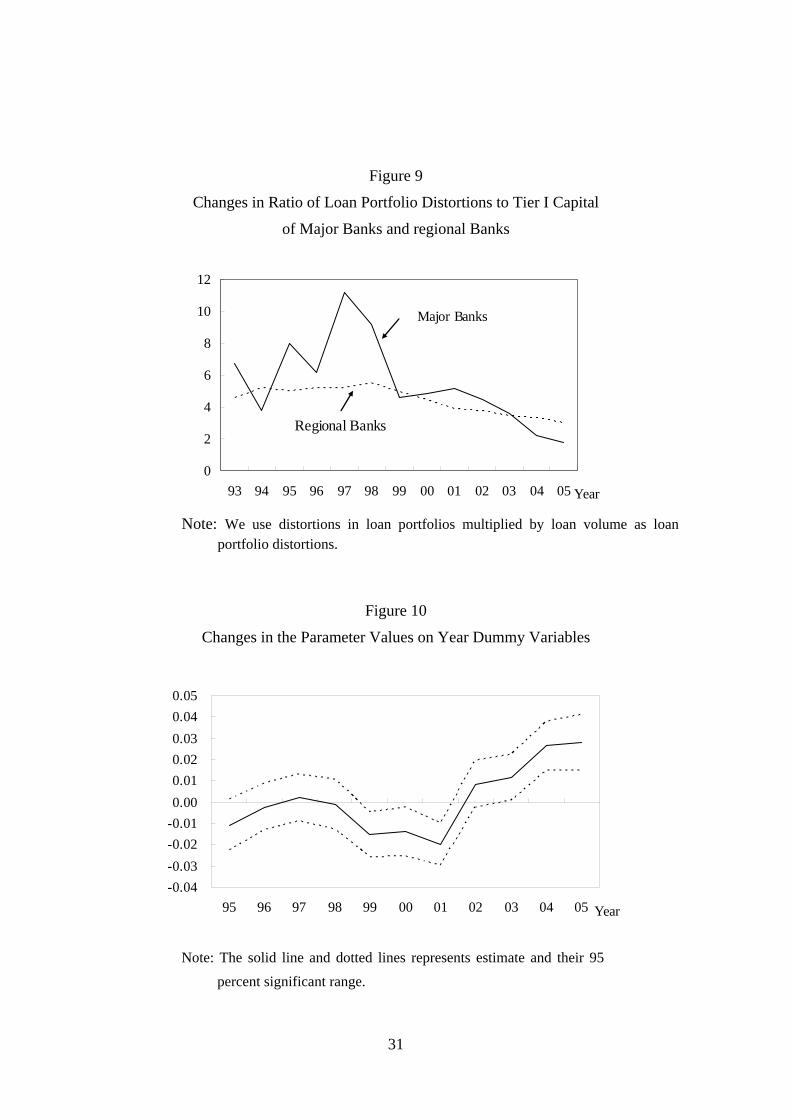
Then, we compare the distortions in loan portfolios and banks’ Tier I capital in
both major banks and regional banks to examine banks’ financial intermediation
functioning. On the one hand, the loan portfolio distortions for major banks drastically
worsened in the late 1990s and those for major banks and regional banks have improved
in the 2000s. On the other hand, Tier I capital held by major banks increased in 1999
owing to injection of public funds, followed by a decrease due to aggressive disposal of
non-performing loans, and increases since 2003, while Tier I capital of regional banks
remained almost unchanged (Figure 8). As a result, the ratios of loan portfolio
distortions to Tier I capital in regional banks were not that high and have declined
moderately since 1999. As for the major banks, the ratios sharply rose in the late 1990s
reflecting the drastic worsening of loan portfolio distortions, regardless of injection of
public funds. This observation suggests that potential imbalances accumulated
especially in major banks and thus the financial system was destabilized in the late
1990s, resulting in the malfunctioning of its financial intermediation function. In the
2000s, risks held by both major banks and regional banks have been contained and
banks have enough capacity to positively fulfill their financial intermediation function
(Figure 9).
IV. Relation between Distortions in Resource Allocation and Distortions in Bank Loan Portfolios
The real distortion estimated in Section II (see Figure 2) and the financial distortion
estimated in the previous section (see Figure 3) show similar movements, although both
distortions are estimated by completely different methods, suggesting a possible relation
between them. In this section, we empirically investigate whether any interaction exists
between them, using data at individual bank level as well as that at industry level.
A. Effect of Real Distortions on Financial Distortions
Below, we quantitatively investigate the effect of the real distortion on the financial
distortion, using individual banks’ data.
Peek and Rosengren (2005) empirically show that banks under a capital

15
constraint tend to provide additional loans to economically insolvent firms in order to
postpone loss realization into the future. We conduct an empirical analysis to confirm
their findings using the more comprehensive measure of loan portfolio distortions and
the mechanism behind the improvement in loan portfolio distortions in the 2000s. We
estimate the equation below:25
,,1,5
,41,31,21,1,
tktk
tktktktktktkCAPCCRa
CAPaCCRaROEaREADacc×+
+++++=−
−−−
δ
(6)
where subscript k denotes bank. δk and READk are each bank’s loan portfolio distortion
and the real distortion which the bank faces, respectively, and higher values mean
higher distortions.26 ROE is ROE based on net operating profits from the core
business27 and CCR is credit cost rate. CAP is a dummy variable that takes one if the
bank’s capital ratio is less than 2 percentage points above the required capital ratio and
zero if not, as is used in Peek and Rosengren (2005). The required capital ratios for
international standard banks and domestic standard banks are 8% and 4%, respectively.
Suppose that banks under capital constraint and with high credit cost are likely to delay
necessary responses to their loan portfolio distortions, resulting in an increase in loan
portfolio distortions. In this case, the parameter on the interaction term between CCR
and CAP is positive. In the estimation, we add year dummy variables as explanatory
variables and use the data for 129 banks that include bankrupted and consolidated banks
in the past for the period from 1993 to 2005.
Table 4 summarizes the estimation results for the fixed effect model.28 The
25 There may be an endogeneity problem. Since we do not have proper instrumental variables, we use a one-year lag in the estimation to avoid the problem.
26 We use the degree of divergence of indicator for distortions in the resource allocation estimated in Section II (γ) in calculating READk. That is, we use the degree of divergence of γ from unity if γ is larger than unity and the degree of divergence of its reciprocal from unity if γ is less than unity. As for READk, for major banks it is the weighted average using disaggregated industrial nominal GDP as weight. READk for regional banks is the weighted average with industrial nominal GDP in the prefecture where the bank’s headquarter is located as weight.
27 Net operating profits from core business are calculated as follows: net operating profits – net realized bond related gains/losses + net transfers to allowances for possible loan losses + loan write-offs in trust account. ROE represents profitability in the core business.
28 Since the Hausman test statistic is 28.30 and the corresponding p-value is 0.00, the fixed effect

16
estimated coefficient for READ is significantly positive, implying that larger real
distortions lead to larger loan portfolio distortions. The coefficient for ROE is
statistically insignificant, even though higher profitability implies larger funds for
disposing of non-performing loans, thus possibly inducing low loan portfolio distortions.
The coefficient for CCR is significantly negative, suggesting that higher credit cost
induces banks to restrain loans to firms with high default risk, thereby reducing loan
portfolio distortions. The coefficient for CAP is significantly negative, showing that
banks under a capital constraint tend to reduce distortions in their loan portfolio. The
coefficient for the interaction term between CCR and CAP is, as expected, significantly
positive. This result demonstrates that banks under capital constraint and with high
credit cost tend to delay disposing of their loans to insolvent firms in order to avoid
incurring additional credit costs.
Focusing on the parameters on the year dummies, they were negative from 1999
to 2001 and have been positive since 2003 (Figure 10). The reason why they have been
positive since 2003 is that distortions in loan portfolios have increased due to the recent
increase in real estate non-recourse loans.29 Negative parameter values from 1999 to
2001 suggest that banks’ behavior dramatically changed in the early 2000s.30
B. Effect of Financial Distortions on Real Distortions
We next estimate the equation below using industry level data to analyze whether an
increase in financial distortions worsens real distortions:31, 32
model was selected.
29 In order to confirm this result, we estimate equation (6) using the data for individual banks’ distortions estimated on the assumption that the loan share to the real estate industry is constant from 2003. In this case, the parameters on the year dummies were significantly negative in 2001 and have been positive but statistically insignificant since 2003.
30 In the early 2000s the Financial Services Agency introduced the Bank Examination Manual and began special inspections of major banks according to the Manual. This change in the stance of financial policy may affect the changes in banks’ behavior. More empirical examinations are needed to confirm this conjecture.
31 In the estimation, we use the data for 12 industries whose real economic and loan portfolio distortions are estimated: food products and beverages, textiles, chemicals, basic metals, machinery, transport equipment, construction, electricity, gas and water supply, wholesale and retail trade, real
17
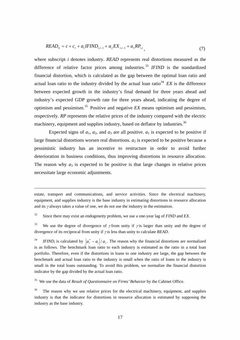
titititit RPaEXaIFINDaccREAD ,31,21,1 ++++= −− , (7)
where subscript i denotes industry. READ represents real distortions measured as the
difference of relative factor prices among industries.33 IFIND is the standardized
financial distortion, which is calculated as the gap between the optimal loan ratio and
actual loan ratio to the industry divided by the actual loan ratio34 EX is the difference
between expected growth in the industry’s final demand for three years ahead and
industry’s expected GDP growth rate for three years ahead, indicating the degree of
optimism and pessimism.35 Positive and negative EX means optimism and pessimism,
respectively. RP represents the relative prices of the industry compared with the electric
machinery, equipment and supplies industry, based on deflator by industries.36
Expected signs of a1, a2, and a3 are all positive. a1 is expected to be positive if
large financial distortions worsen real distortions. a2 is expected to be positive because a
pessimistic industry has an incentive to restructure in order to avoid further
deterioration in business conditions, thus improving distortions in resource allocation.
The reason why a3 is expected to be positive is that large changes in relative prices
necessitate large economic adjustments.
estate, transport and communications, and service activities. Since the electrical machinery, equipment, and supplies industry is the base industry in estimating distortions in resource allocation and its γ always takes a value of one, we do not use the industry in the estimation.
32 Since there may exist an endogeneity problem, we use a one-year lag of FIND and EX.
33 We use the degree of divergence of γ from unity if γ is larger than unity and the degree of divergence of its reciprocal from unity if γ is less than unity to calculate READ.
34 IFINDi is calculated by iii aaa /* − . The reason why the financial distortions are normalized is as follows. The benchmark loan ratio to each industry is estimated as the ratio in a total loan portfolio. Therefore, even if the distortions in loans to one industry are large, the gap between the benchmark and actual loan ratio to the industry is small when the ratio of loans to the industry is small in the total loans outstanding. To avoid this problem, we normalize the financial distortion indicator by the gap divided by the actual loan ratio.
35 We use the data of Result of Questionnaire on Firms’ Behavior by the Cabinet Office.
36 The reason why we use relative prices for the electrical machinery, equipment, and supplies industry is that the indicator for distortions in resource allocation is estimated by supposing the industry as the base industry.

18
Since industries with large distortions and small distortions may behave
differently, we split the data into two groups: 6 industries with the largest distortions in
resource allocation and the other 6 industries with the smallest distortions, and estimate
equation (7) for each group. We employ the pooled OLS estimation and incorporate
year dummies in estimating equation (7).
Table 5 shows the estimation results. First, the parameter on financial distortions
for industries both with large and small real distortions is positive and statistically
significant, demonstrating that financial distortions worsen real distortions. The
parameter value on financial distortions for industries with large real distortions is
larger than that with small real distortions. Second, the parameters on expectation on
future economic condition are negative for industries with large real distortions but
positive and statistically significant for those with small real distortions. This result
implies that sectors with small real distortions execute restructuring to reduce their
distortions when they become pessimistic about their future economic condition but
sectors with large real distortions do not execute sufficient restructuring even though
they are pessimistic. Third, the parameters on relative price are positive and statistically
significant for industries with large real distortions but statistically insignificant for
those with small distortions.
C. Summary of Empirical Results
The above empirical analyses confirm the existence of interaction between real and
financial distortions. The panel data analyses using data at individual bank level as well
as that at industry level show that negative interaction existed between real and financial
distortions in the late 1990s, but such negative interaction became positive, in which the
improvement of financial distortion induced a decrease in real distortions, after the end
of the 1990s. This finding suggests that in the 2000s, banks changed their lending
behavior, as did recipient firms such as by cutting excess debt and taking measures to
raise profitability.
V. Concluding Remarks
In this paper, we have empirically analyzed the interaction between the real and
19
financial distortions during the period of Japan’s protracted economic stagnation after
the 1990s. In doing so, we have focused on the protracted economic stagnation after the
bursting of the asset price bubble, and the subsequent recovery in economic activity and
restoration of financial system stability. Our empirical evidence suggests two points.
First, both distortions in factor markets and banks’ loan portfolios drastically
deteriorated in the late 1990s, followed by remarkable improvement in the 2000s.
Second, negative interaction existed between the two distortions in the late 1990s, but
such negative interaction reversed and became positive in the 2000s.
The real distortion induced a decline in trend growth rates for an extended
period of time due to a contraction of production possibility frontier by keeping troubled
firms alive, and inefficient resource allocation in an intertemporal dimension through a
slowdown in capital accumulation.37 In addition, the financial distortion, accumulated
in the banking sector as potential imbalances, suddenly materialized when a certain
threshold was reached. The risk-smoothing function of the banking system was then
suddenly lost when the system encountered a shock that eroded banks’ net capital to the
extent that it threatened their soundness. Moreover, the negative interaction between the
real and financial distortions exacerbated adverse effects on the economy: the
destabilized financial system worsened the misallocation of resources, thereby further
destabilizing the financial system.
The market mechanism alone, however, is unable to resolve the real and
financial distortions, since resolution of the distortions tends to put someone at a
disadvantage. As a result, resource misallocation is likely to continue to exist. In
particular, financial system instability makes it more difficult to resolve resource
misallocations by the market mechanism alone. That is, under the circumstances where
banks’ capital positions are deteriorated and the financial system become unstable, loans
to unprofitable firms become fixed and funds are not channeled to growing firms,
thereby producing downward pressure on economic activity. It is crucially important to
induce efficient resource allocation through macroeconomic policy including prudential
policy in order to achieve not only financial system stability but also sustained
37 See Okina and Shiratsuka (2005) on this point.

20
economic growth.38
38 Bhagwati (1971) argues that the basic policy response to structural problems is to attack directly their sources by transferring economic resources between agents gaining and those losing from structural reform.

21
References
Allen, Franklin, and Douglas Gale, “Financial Markets, Intermediaries, and
Intertemporal Smoothing,” The Journal of Political Economy 105(3), 1997, pp.
523–546.
Bhagwati, Jagdish, “The Generalized Theory of Distortion and Welfare,” in Jagdish
Bhagwati ed., Trade, Balance of Payments, and Growth: Papers in International
Economics in Honor of Charles P. Kindleberger, Amsterdam: North-Holland,
1971, pp. 98–116.
Buch, Claudia M., John C. Driscoll, and Charlotte Ostergaar, “Cross-Border
Diversification in Bank Asset Portfolios,” Finance and Economics Discussion
Paper Series 2004-26, Federal Reserve Board, 2004.
Caballero, Ricardo J., Takeo Hoshi, and Anil K. Kashyap, “Zombie Lending and
Depressed Restructuring in Japan,” NBER Working Paper 12129, National Bureau
of Economic Research, 2006.
Fukao, Kyoji, et al., “Sangyobetsu Seisansei to Keizaiseicho: 1970–1998 (Productivity
and Economic Growth by Industry: 1970-1998),” Keizai Bunseki (Economic
Analysis), 170, Economic and Social Research Institute, Cabinet Office, 2003 (in
Japanese).
Hayashi, Fumio, and Edward C. Prescott, “The 1990s in Japan: A Lost Decade,” Review
of Economic Dynamics, 5, 2002, pp. 206–235.
Hoshi, Takeo, “Economics of the Living Dead,” The Japanese Economic Review, 57(1),
2006, pp. 30–49.
______, and Anil K. Kashyap, “The Japanese Banking Crisis: Where Did It Come from
and How Will It End?” in Ben S. Bernanke and Julio Rotemberg, eds., NBER
Macroeconomics Annual 1999, Vol. 14, Cambridge, MA. and London: MIT Press,
2000, pp. 129–201.
Johnson, Harry G., “Factor Market Distortions and the Shape of the Transformation
Curve,” Econometrica, 34, 1966, pp. 686–698.
Jones, Ronald W., “Distortions in Factor Markets and the General Equilibrium Model of
Production,” The Journal of Political Economy, 79, 1971, pp. 437–459.
Kawamoto, Takuji, “What Do the Purified Solow Residuals Tell Us about Japan’s Lost
Decade?” Monetary and Economic Studies, 23(1), Institute for Monetary and

22
Economic Studies, Bank of Japan, 2005, pp. 113–148.
Maeda, Eiji, Masahiro Higo, and Kenji Nishizaki, “Wagakuni no ‘Keizai Kozo Chosei’
nitsuiteno Ichikosatsu (A Study on ‘Economic Structural Adjustments’ in Japan),”
Nippon Ginko Chousa Geppo (Bank of Japan Monthly Bulletin), July, 2001 (in
Japanese).
Miyagawa, Tsutomu, “Seisansei no Keizaigaku: Wareware no Rikai ha Dokomade
Susundaka (Economics on Productivity: How Far Do We Understand?),” Nippon
Ginkou Working Paper Series No. 60-J-06, Nippon Ginkou, 2006 (in Japanese).
Nagahata, Takashi, and Toshitaka Sekine, “Firm Investment, Monetary Transmission
and Balance-sheet Problems in Japan: An Investigation Using Micro Data.” Japan
and World Economy, 17, 2005, pp. 345–369. Nakakuki, Masayuki, Akira Otani, and Shigenori Shiratsuka, “Distortions in Factor
Markets and Structural Adjustments in the Economy,” Monetary and Economic
Studies, 22(2), Institute for Monetary and Economic Studies, Bank of Japan, 2004,
pp. 71–100.
Okina, Kunio, and Shigenori Shiratsuka, “Asset Price Bubbles, Price Stability, and
Monetary Policy: Japan’s Experience,” Monetary and Economic Studies, 20(S-1),
Institute for Monetary and Economic Studies, Bank of Japan, 2002, pp. 35–76.
______, and ______, “Asset Price Fluctuations, Structural Adjustments, and Sustained
Economic Growth: Lessons from Japan’s Experience since Late 1980s,” Monetary
and Economic Studies, 22(S-1), Institute for Monetary and Economic Studies,
Bank of Japan, 2004, pp. 143–177.
Peek, Joe, and Eric S. Rosengren, “Unnatural Selection: Perverse Incentives and the
Misallocation of Credit in Japan,” American Economic Review, 95(4), 2005, pp.
1144–1166.
Saito, Makoto, Seichou Shinkou no Shikkoku: Syouhi Jyoushi no Macro Keizaigaku
(Chain of Belief in Economic Growth: Macroeconomics Attaching Greater
Importance to Consumption), Keisoushobou, 2006 (in Japanese).
Sekine, Toshitaka, Keiichiro Kobayashi, and Yumi Saita, “Forbearance Lending: The
Case of Japanese Firms,” Monetary and Economic Studies, 21(2), Institute for
Monetary and Economic Studies, Bank of Japan, 2004, pp. 69–92.
Syrquin, Moshe, “Productivity and Factor Reallocation,” in H. Chenery, R. Sherman

23
and M. Syrquin eds., Industrialization and Growth: A Comparative Study, Oxford
University Press, 1986.
24
Table 1
Decomposition of Japan’s GDP Growth Rate
(%)
1986–91
(a)
1992–2000
(b)
2001–04
(c)
(b)-(a)
(c)-(b)
GDP growth rate 4.71 1.23 1.14 -3.48 -0.09
TFP 2.05 0.78 0.96 -1.27 0.18
Labor input 0.39 -0.67 -0.79 -1.06 -0.12
Capital accumulation 2.26 1.12 0.97 -1.14 -0.15
Distortions 0.42 0.10 0.17 -0.31 0.06
Factor’s marginal productivity (γ) 0.05 -0.19 0.12 -0.24 0.31
Labor input share 0.36 0.29 0.04 -0.07 -0.25
Table 2
Relation between Distortions in Loan Portfolios and Non-performing Loan Ratio
1-year lag 2-year lag 3-year lag
FIND-j 15.02***(9.94) 15.53***(6.35) 9.77***(3.39)
R2 0.63 0.63 0.61
Note: Estimation was conducted using the data for 138 banks. Estimation period is 1999–2005. *** denotes 1 percent significance level. Figures in parentheses are t-statistics.

25
Table 3
Comparison of Ratios of Loan Portfolio Distortions to
Tier I Capital of Bankrupted or Consolidated Banks with Those of Existing Banks
Average Std.
Bankrupted or Consolidated
Banks
10.17(a) 7.63
Existing Banks 5.70 (b) 7.97
t-statistic [Test on the null hypothesis that (a)
is equal to (b)]
14.78
Note: Data for bankrupted or consolidated banks (15 banks) are those of the year before they were bankrupted or consolidated. Data for existing banks (99 banks) are the maximum value from 1993 to 2005. Note that we use distortions in loan portfolios multiplied by loan volume as loan portfolio distortions.
Table 4
Estimation Results of Equation (6)
Dependent Variable: δ READ-1 9.579*** (4.11) ROE-1 -0.002 (0.11) CCR-1 -0.002** (2.51) CAP -1.392*** (2.92) CCR-1*CAP 0.005* (4.07) R2 0.51
Note: Estimation is conducted using data for 129 banks
(1993–2005). ***, **, and * represent 1 percent, 5 percent, and 10 percent significance level, respectively. Figures in parentheses are t-statistics.

26
Table 5
Estimation Results of Equation (7)
Dependent Variable: READ Industry with higher
distortion Industry with lower
distortion -10.78** 0.22 c
(2.22) (0.26) 0.72* 0.32*** IFIND-1 (1.82) (3.97) -0.35 0.19*** EX-1 (1.62) (4.61) 0.16*** -0.00 RP-1 (2.90) (0.12)
R2 0.23 0.53
Note: Industries with higher distortion are Food products and beverages, Mining, Construction, Electricity, gas and water supply, Wholesale and retail trade, and Transport and communications. Industries with lower distortion are Chemicals, Basic metals, Machinery, Transport equipment, Real estate, and Service activities. ***, **, and * represent 1 percent, 5 percent, and 10 percent significance level, respectively. Figures in parentheses are t-statistics.
27
Figure 1
Changes in Industrial Distortions in Resource Allocation
01
23
456
78
910
Agr
icul
ture
, for
estry
, and
fish
erie
s
Min
ing
Food
pro
duct
s and
bev
erag
es
Text
iles
Pulp
, pap
er, a
nd p
aper
pro
duct
s
Chem
ical
s
Petro
leum
and
coa
l pro
duct
s
Non
met
alic
min
eral
pro
duct
s
Basic
met
als
Fabr
icat
ed m
etal
pro
duct
s
Mac
hine
ry
Elec
trica
l mac
hine
ry, e
quip
mep
t, an
d
Tran
spor
t equ
ipm
ent
Prec
ision
instr
umen
ts
Oth
er m
anuf
actu
ring
Cons
truct
ion
Elec
trici
ty, g
as, a
nd w
ater
supp
ly
Who
lesa
le a
nd re
tail
trade
Fina
nce
and
insu
ranc
e
Real
esta
te
Tran
spor
t and
com
mun
icat
ions
Serv
ice
activ
ities
199020002004
Figure 2
Distortion in Resource Allocation in the Whole Economy
1.0
1.2
1.4
1.6
1.8
2.0
2.2
2.4
90 91 92 93 94 95 96 97 98 99 00 01 02 03 04Year
Note: In computing the weighted average of γs with nominal GDP, we use γs’ degree of divergence from unity if it exceeds unity and the degree of divergence of its reciprocal from unity if it is less than unity.
28
Figure 3
Benchmark Loan Portfolios and Actual Loan Portfolios
Figure 4
Changes in Distortions in Loan Portfolios
0.15
0.20
0.25
0.30
0.35
0.40
93 94 95 96 97 98 99 00 01 02 03 04 05
Gap in Loans toAll Industries
Gap in Loans toManufacturing industries
Year
Gap in Loans to Non-manufacturing industries
Return
Risk
Efficient frontier
Benchmark loan portfolio
Actual loan portfolio
29
Figure 5
Changes in Loan Portfolio Distortions in Major Banks and Regional Banks
0.20
0.25
0.30
0.35
0.40
93 94 95 96 97 98 99 00 01 02 03 04 05 Year
Major Banks
Regional Banks
Note: Weighted average using loan volume as weight.
Figure 6
Loan Portfolio Distortions Adjusting Loans to the Real Estate Industry
0.20
0.25
0.30
0.35
0.40
93 94 95 96 97 98 99 00 01 02 03 04 05 Year
Major Banks
Whole Banking Sector
Regional Banks

30
Figure 7
Relationship between Loan Portfolio Distortions and Non-performing Loan Ratio
0.20
0.22
0.24
0.26
0.28
0.30
0.32
0.34
92 93 94 95 96 97 98 99 00 01 02 03 04 050.01.02.03.04.05.06.07.08.09.010.0
Loan Distortions(left scale)
Nonperforming LoanRatio (right scale)
Year
%
Note: Non-performing loan ratio is defined as risk-monitored loans divided by total loans
outstanding. Data for risk-monitored loans are published by FSA. Before 1994, they are the sum of bankrupt assets and delinquent assets, and in 1995 and 1996 they are the sum of bankrupt assets, delinquent assets and restructured loans. Note that data for loan portfolio distortions are those by calendar year, and data for non-performing loans are by fiscal year.
Figure 8
Changes in Tier I Capital Held by Major Banks and Regional Banks
0.0
5.0
10.0
15.0
20.0
93 94 95 96 97 98 99 00 01 02 03 04 05
Major Banks
Regional Banks
Fiscal year
Trillion Yen
Note: Data for international standard banks are Tier I capital, and those for domestic standard
banks are the sum of common stock, capital surplus reserve, and earned surplus.
31
Figure 9
Changes in Ratio of Loan Portfolio Distortions to Tier I Capital
of Major Banks and regional Banks
0
2
4
6
8
10
12
93 94 95 96 97 98 99 00 01 02 03 04 05
Major Banks
Regional Banks
Year
Note: We use distortions in loan portfolios multiplied by loan volume as loan portfolio distortions.
Figure 10
Changes in the Parameter Values on Year Dummy Variables
-0.04-0.03-0.02-0.010.000.010.020.030.040.05
95 96 97 98 99 00 01 02 03 04 05 Year
Note: The solid line and dotted lines represents estimate and their 95 percent significant range.