Technical Report 2009-001

Distance to set operations in constructive modeling of

solids

Pierre-Alain Fayolle

August 19, 2009

Computer Graphics Laboratory

The University of AizuTsuruga, Ikki-Machi, Aizu-Wakamatsu City

Fukushima, 965-8580 Japan

Technical Report 2009-001

Title:

Authors:

Key Words and Phrases:

Abstract:

Report Date: Written Language:

Any Other Identifying Information of this Report:

Distribution Statement:

Supplementary Notes:

The University of Aizu

Aizu-Wakamatsu

Fukushima 965-8580

Japan

8/19/2009 English

First Issue: 10 copies

Pierre-Alain Fayolle

Distance to set operations in constructive modeling of solids

implicit surfaces, distance function, constructive modeling, set operations

We propose in this paper methods to compute the signed distance to surface obtained by theintersection (respectively union, difference) of two solids (in two and three dimensions). Theseimplementations can replace “min/max” or “R-functions” used to model set operations onimplicit surfaces.

Computer Graphics Laboratory

Distance to set operations in constructive modeling

of solids

Pierre-Alain Fayolle

08/04/2009

Contents

1 Introduction 2

1.1 Related works . . . . . . . . . . . . . . . . . . . . . . . . . . . 21.1.1 The distance function . . . . . . . . . . . . . . . . . . 21.1.2 Constructive geometry with real valued functions . . . 3

1.2 Overview and main contributions . . . . . . . . . . . . . . . . 4

2 Construction of the intersection in two dimensions 4

2.1 Intersection to two orthogonal halfspaces . . . . . . . . . . . . 52.2 Determination of the space where min does not give the exact

distance . . . . . . . . . . . . . . . . . . . . . . . . . . . . . . 52.3 Determination of the closest point . . . . . . . . . . . . . . . 62.4 Distance to the intersection . . . . . . . . . . . . . . . . . . . 72.5 Extension to union and difference . . . . . . . . . . . . . . . . 8

3 Construction of the intersection in three dimensions 8

3.1 Determination of the closest point . . . . . . . . . . . . . . . 83.2 Distance to the intersection . . . . . . . . . . . . . . . . . . . 9

4 Results and discussions 9

4.1 Visualization of distance fields . . . . . . . . . . . . . . . . . . 94.1.1 Contour field in two dimensions . . . . . . . . . . . . . 104.1.2 Contour field on planar section in three dimensions . . 104.1.3 Discussion . . . . . . . . . . . . . . . . . . . . . . . . . 11

5 Conclusion 13

Abstract

We propose in this paper methods to compute the signed distanceto surface obtained by the intersection (respectively union, difference)of two solids (in two and three dimensions). These implementationscan replace “min/max” or “R-functions” used to model set operationson implicit surfaces.

1

1 Introduction

In geometric modeling, a solid can be defined by the sign of a function:the set {p : f(p) ≥ 0} defines the interior and the boundary, and the set{p : f(p) < 0} the exterior (see [4] on implicit surfaces, [1] on FunctionRepresentation and the references therein). The case where f is the signedEuclidean distance to the boundary of the solid f = 0 is of special interest.Distance based models are extremely useful in many applications such as:constant-radius offsetting and blending operations [16], surface metamor-phosis and smoothing [13], object reconstruction from a set of cross-sections[10], rendering with sphere tracing [6], generation of skeletal shape repre-sentation [23], heterogeneous object modeling [3], and others. We proposein this paper methods for calculating the signed Euclidean distance froma point to the surface of a solid constructed by applying set-theoretic op-erations (union, intersection, difference) to primitives defined by distancefunctions. That is: if d1 and d2 represent the distance to the surface of twoprimitives S1 and S2, we propose algorithms to calculate the distance d tothe union (respectively intersection, difference) of S1 and S2.

1.1 Related works

1.1.1 The distance function

Let d(p), p ∈ R3 be the signed distance function to an oriented closedsurface M . The function d is the vanishing viscosity solution of the Eikonalequation [22, 21, 19]:

‖∇d‖2 = 1, d|M = 0 (1)

where ‖.‖2 is the Euclidean norm. Let c be the closest point of p in thesurface M , the signed distance is then ε‖p − c‖2, where ε = −1 if p isoutside M . If the surface is smooth, then p− c is orthogonal to the surface.The signed Euclidean distance function is at least C 0, and may be notdifferentiable at some points.

Expressions for the distance function to most of the classic surfaces of aCSG system (sphere, cylinder, cone) are known analytically [6] and distanceto general quadrics and ellipsoids can be computed by a numerical procedure[7].

In general, if the surface M is available as an oriented point-set or a meshof polygons, it is possible to solve the Eikonal equation (1) on a finite grid.There exists various optimal numerical algorithms such as the fast marchingmethod [19], the fast sweeping method [21, 22], or the characteristics / scanconversion algorithm [11]. Algorithms, that exploit the GPU, have also beendesigned in order to compute efficiently the Euclidean distance function[8, 20]. After a grid is obtained with the signed Euclidean distance to M

2

in each of its nodes, it is always possible to apply spline interpolation /approximation, to get an analytical expression [15].

1.1.2 Constructive geometry with real valued functions

In constructive geometry, complex solids are built by applying successivelyset-theoretic operations (union, intersection, difference) to primitives. Whensolids are described by real valued functions, like in implicit surfaces or F-Rep, expressions for set-theoretic operations have been proposed by Sabin[18], Ricci [14] and Rvachev [17]. Sabin [18] and Ricci [14], independentlyproposed the use of “min/max”. If d1 and d2 are the functions definingtwo solids, then the union is defined by the function max(d1, d2 and theintersection by min(d1, d2) (the difference is obtained from the intersectionby replacing d2 by −d2). Rvachev proposed the “R-functions” [17]:

d1 ∨α d2 = 11+α

(d1 + d2 +√

d21 + d2

2 − 2αd1d2)

d1 ∧α d2 = 11+α

(d1 + d2 −√

d21 + d2

2 − 2αd1d2)(2)

Neither ”min/max” nor the R-functions keep the distance to the con-structed solid. This is illustrated in Fig. 1, where the approximate distanceto the surface made by the intersection of the halfspaces: x ≥ 0 and y ≥ 0is computed with an ”R-function” on the left and ”min” on the right.

−2 −1.5 −1 −0.5 0 0.5 1 1.5 2−2

−1.5

−1

−0.5

0

0.5

1

1.5

2

−2 −1.5 −1 −0.5 0 0.5 1 1.5 2−2

−1.5

−1

−0.5

0

0.5

1

1.5

2

Figure 1: Approximate distance to the intersection of the halfspaces x ≥ 0and y ≥ 0. Left: R-function is used to implement the intersection. Right:Min is used.

”Min/max” tend however to keep a better approximation of the distancethan the ”R-functions”. This can be illustrated by computing the union ofa disk with itself and looking at the value of the function (union of thedisks) at the center. The distance to a circle of radius 1 and center [0, 0]is: d(p) = 1.0 −

√

p2, and the union of the disk with itself is defined by:

3

max(d(p), d(p)) or: d(p) ∨0 d(p). In the former case, the distance at thecenter is: 1.0 while in the latter it is: 3.41421.

The functions “min/max” are not differentiable on the set of points corre-sponding to the equality of their arguments. Because of this, “R-functions”are sometimes preferred; ”R-functions” are not differentiable only on the setof points where their arguments are both equal to 0. This property of the“R-functions” is used for example when implementing a blending effect [12].

Some works tried to address this issue by modifying the contour lines ofthe functions min(x, y) and max(x, y): functions proposed in the work [9, 2]were designed for blending, while [5] were designed for keeping the distanceapproximation of ”min/max” while removing the points where the functionis not C1.

1.2 Overview and main contributions

The main contributions of this paper are methods to compute in two andthree dimensions the distance to solids defined by the union (respectivelyintersection, difference) of solids defined by distance functions. That is: if S1

and S2 are solids defined by the distance functions d1 and d2, we describemethods to compute d the signed distance to S = S1 ∪ S2 (respectivelyS1 ∩ S2 and S1\S2). These expressions for the set-theoretic operations canbe used instead of ”min/max” or the ”R-functions” in implicit surfaces orF-Rep modeling systems.

Union and intersection are dual, and the difference is obtained from theintersection, so we will limit the discussion to the construction of an expres-sion for the intersection. We first describe the method in two dimensions,when d1 and d2 are functions in R2. Then, we explain how to modify themethod for the three dimensional case. Finally, we illustrate through exam-ples in two and three dimensions the behavior of these functions and howthey compare against ”min/max” or ”R-functions”.

2 Construction of the intersection in two dimen-

sions

In this section, we describe how to get an expression for computing theintersection of two shapes defined by signed distance functions. We start byan example: the intersection of two orthogonal halfspaces x ≥ 0 and y ≥ 0(as illustrated in Fig. 1), and explain how the scalar field constructed bymin(x, y) differs from the signed distance to the intersection. We generalizethe method to the intersection of any objects defined by their signed distancefields: d1(x, y) and d2(x, y).

4

2.1 Intersection to two orthogonal halfspaces

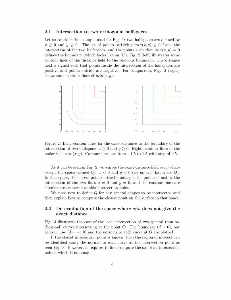
Let us consider the example used for Fig. 1: two halfspaces are defined byx ≥ 0 and y ≥ 0. The set of points satisfying min(x, y) ≥ 0 forms theintersection of the two halfspaces, and the points such that min(x, y) = 0defines the boundary (which looks like an ’L’). Fig. 2 (left) illustrates somecontour lines of the distance field to the previous boundary. The distancefield is signed such that points inside the intersection of the halfspaces arepositive and points outside are negative. For comparison, Fig. 2 (right)shows some contour lines of min(x, y).

−2 −1.5 −1 −0.5 0 0.5 1 1.5 2−2

−1.5

−1

−0.5

0

0.5

1

1.5

2

−2 −1.5 −1 −0.5 0 0.5 1 1.5 2−2

−1.5

−1

−0.5

0

0.5

1

1.5

2

Figure 2: Left: contour lines for the exact distance to the boundary of theintersection of two halfspaces x ≥ 0 and y ≥ 0. Right: contour lines of thescalar field min(x, y). Contour lines are from −1.5 to 1.5 with step of 0.5.

As it can be seen in Fig. 2, min gives the exact distance field everywhereexcept the space defined by: x < 0 and y < 0 (let us call that space Q).In that space, the closest point on the boundary is the point defined by theintersection of the two lines x = 0 and y = 0, and the contour lines arecircular arcs centered at this intersection point.

We need now to define Q for any general shapes to be intersected andthen explain how to compute the closest point on the surface in that space.

2.2 Determination of the space where min does not give the

exact distance

Fig. 3 illustrates the case of the local intersection of two general (non or-thogonal) curves intersecting at the point O. The boundary (d = 0), onecontour line (d = −1.0) and the normals to each curve at O are plotted.

If the closest intersection point is known, then the region of interest canbe identified using the normal to each curve at the intersection point asseen Fig. 3. However, it requires to first compute the set of all intersectionpoints, which is not easy.

5

−2 −1.5 −1 −0.5 0 0.5 1 1.5 2−2

−1.5

−1

−0.5

0

0.5

1

1.5

2

Figure 3: Local intersection of two general curves. Curve resulting of theintersection, one contour line at the distance −1.0 and the normals to eachcurve at the intersection point.

We will proceed in the reverse way by first determining the space ofinterest and then computing the closest intersection point in that space.

Given a point p ∈ R2 (see as an illustration Fig. 4), we first calculatesthe projection p1 of p on the first curve c1. Using the signed distance fieldd1 to the curve and its gradient, the projection is given by:

p1 ← p− d1(p)∇d1(p) (3)

Similarly, we calculate p2 the projection of p on the second curve c2.p belongs to the zone of interest Q, if d1(p2) < 0 and d2(p1) < 0.

2.3 Determination of the closest point

If the current point of evaluation p0 is in Q, then the next step is to computeits closest point p on the boundary of the intersection. The closest point isat the intersection of the two curves:

L(p) =

[

d1(p) = 0d2(p) = 0

]

(4)

This system is solved for p = (x, y) by using the damped Newton methodwith the initial guess p0. Eq. 5 is iterated until the residual L(pk) is small,and p is set to pk.

6

Figure 4: Two curves c1 and c2 (solid lines) defined by the distance fields d1

and d2. A given point p and the contour lines of d1 and d2 passing throughp. p1 and p2 the projections of p on c1 and c2.

pk+1 = pk − αJ−1(pk)L(pk) (5)

where α is the damping factor, and J is the Jacobian matrix of L.

J(p) =

(

∂d1

∂x(p) ∂d1

∂y(p)

∂d2

∂x(p) ∂d2

∂y(p)

)

(6)

Because p0 is close to p, pk converges relatively fast.

2.4 Distance to the intersection

Putting together the results of the previous subsections, a procedure forcalculating the distance to the intersection of two curves defined by thesigned distance functions is:

distInter Given a point p ∈ R2, and two (2D) solids defined by the signeddistance functions d1 ≥ 0 and d2 ≥ 0, compute the distance to the curve,boundary of the intersection of the two solids.

1. [distance to curve 1] d1 = d1(p)2. [distance to curve 2] d2 = d2(p)3. [normal to d1] n1 = ∇d1(p)4. [projection on curve 1] p1 = p− d1n1

7

5. [normal to d2] n2 = ∇d2(p)6. [projection on curve 2] p2 = p− d2n2

7. [in Q?] inQ? = d1(p2) < 0 AND d2(p1) < 08. if (inQ? is true) then:

(a) [closest point] pc = closestInter(p, d1(.), d2(.)) (see section 2.3)(b) [distance] d = −‖p− pc‖2

9. else:

(a) [distance] d = min(d1, d2)

10. [return] return d

2.5 Extension to union and difference

The distance to the union is similar except for:

• the section 2.2 (step 7 of the algorithm distInter in section 2.4), wherethe condition d1(p2) < 0 AND d2(p1) < 0 should be replaced by thecondition d1(p2) > 0 AND d2(p1) > 0,

• the step 8.b) of the algorithm distInter in section 2.4, which should bereplaced by: d = ‖p− pc‖2.

The distance to the set-theoretic difference is obtained by replacing thefunction d2(.) by the function −d2(.) in the algorithm distInter.

In the following section, we extend the method for working with threedimensional objects.

3 Construction of the intersection in three dimen-

sions

The construction of the distance to the intersection in three dimensions issimilar to the two dimensional case. The only difference is in determiningthe closest intersection point.

3.1 Determination of the closest point

In three dimensions, the system in eq. 4 has three unknowns (x, y and z)but only two equations. The third equation is obtained by observing thatthe closest intersection point is in the plane containing the gradient of eachfunction at the current point of evaluation (p0). Let n1 = ∇d1(p0) andn2 = ∇d2(p0) be the gradients of d1 and d2 at p0. The third equationbecomes: n(p−p0) = 0, where n = n1∧n2. We have to solve the followingsystem:

L(p) =

d1(p) = 0d2(p) = 0n(p− p0) = 0

(7)

8

This is solved with the damped Newton method as in section 2.3. TheJacobian of the system eq. 7 is:

J(p) =

∂d1

∂x(p) ∂d1

∂y(p) ∂d1

∂z(p)

∂d2

∂x(p) ∂d2

∂y(p) ∂d2

∂z(p)

nx ny nz

(8)

where nx, ny and nz are the components of n.

3.2 Distance to the intersection

Putting together the results of the previous subsections, a procedure forcalculating the distance to the intersection of two surfaces defined by signeddistance functions is:

distInter3D Given a point p ∈ R3, and two (3D) solids defined by thesigned distance functions d1 ≥ 0 and d2 ≥ 0, compute the distance to thesurface, boundary of the intersection of the two solids.

1. [distance to surface 1] d1 = d1(p)2. [distance to surface 2] d2 = d2(p)3. [normal to d1] n1 = ∇d1(p)4. [projection on surface 1] p1 = p− d1n1

5. [normal to d2] n2 = ∇d2(p)6. [projection on surface 2] p2 = p− d2n2

7. [in Q?] inQ? = d1(p2) < 0 AND d2(p1) < 08. if (inQ? is true) then:

(a) [closest point] pc = closestInter3D(p, d1(.), d2(.)) (see section3.1)

(b) [distance] d = −‖p− pc‖29. else:

(a) [distance] d = min(d1, d2)

10. [return] return d

4 Results and discussions

4.1 Visualization of distance fields

The distance field to the intersection and union of two solids is illustratedin two and three dimensions in the following examples.

9

4.1.1 Contour field in two dimensions

Fig. 5 illustrates the contour field of the signed distance functions resultingin the intersection of two non-orthogonal planes and two disks. Intersectionwas implemented using: “R-functions” (left), “min/max” (middle) and themethod proposed in this paper. The functions built using “R-functions”do not respect the Euclidean metric. The functions built using “min/max”failed to do so only in the space identified in section 2.2. Compare the resultswith the method proposed here and the circular arcs in the contour linesoutside of the constructed solids.

−2 −1.5 −1 −0.5 0 0.5 1 1.5 2−2

−1.5

−1

−0.5

0

0.5

1

1.5

2

−4

−3.5

−3

−2.5

−2

−1.5

−1

−0.5

0

0.5

−2 −1.5 −1 −0.5 0 0.5 1 1.5 2−2

−1.5

−1

−0.5

0

0.5

1

1.5

2

−2.5

−2

−1.5

−1

−0.5

0

0.5

1

−2 −1.5 −1 −0.5 0 0.5 1 1.5 2−2

−1.5

−1

−0.5

0

0.5

1

1.5

2

−2.5

−2

−1.5

−1

−0.5

0

0.5

1

−2 −1.5 −1 −0.5 0 0.5 1 1.5 2−2

−1.5

−1

−0.5

0

0.5

1

1.5

2

−6

−5

−4

−3

−2

−1

0

−2 −1.5 −1 −0.5 0 0.5 1 1.5 2−2

−1.5

−1

−0.5

0

0.5

1

1.5

2

−2

−1.5

−1

−0.5

0

−2 −1.5 −1 −0.5 0 0.5 1 1.5 2−2

−1.5

−1

−0.5

0

0.5

1

1.5

2

−2

−1.5

−1

−0.5

0

Figure 5: First row: Intersection of two halfplanes using for the intersection(from left to right): “R-functions”, “min”, the method proposed in thiswork. Second row: Intersection of two disks.

Fig. 6 illustrates the contour field of the distance to the union of twohalfplanes (left) and two disks (right) using the method introduced here.

4.1.2 Contour field on planar section in three dimensions

Visualizing scalar fields in three dimensions is more difficult. We visualizeinstead the fields in a planar section. Fig. 7 (right) illustrates the pro-posed method applied in three dimensions to compute the distance to theintersection of two spheres. This should be compared with the sections infig. 7 left and middle obtained with respectively “R-functions” and “min”.Additionally, fig. 8 illustrates the result of the proposed method to computethe distance to the union of two spheres by showing the distance field on asection by the plane y = 0.

10

−2 −1.5 −1 −0.5 0 0.5 1 1.5 2−2

−1.5

−1

−0.5

0

0.5

1

1.5

2

−1

−0.5

0

0.5

1

1.5

2

2.5

−2 −1.5 −1 −0.5 0 0.5 1 1.5 2−2

−1.5

−1

−0.5

0

0.5

1

1.5

2

−1.5

−1

−0.5

0

0.5

Figure 6: Left: distance to the union of two halfplanes with our method.Right: distance to the union of two disks.

Figure 7: Distance to the intersection of two spheres using for the intersec-tion (from left to right): “R-functions”, “min”, the method proposed in thiswork. Second row: Intersection of two disks.

4.1.3 Discussion

As mentioned earlier, the distance function is at least C 0 but not ev-erywhere differentiable; for example, the sphere is not differentiable at itscenter. Our algorithms, as described above, make use of the gradient of thefunctions passed as input. The question is what value of the gradient to usein these cases. The points where the distance function is not differentiablehave more than one closest point on the surface of the solid, and thereforemore than one gradient at that point. The easiest solution is to consistentlypick one gradient from the set of possible gradients. This is the solutionthat was used for the intersection / union of the disks and spheres in theexamples above.

An alternative solution is to use slightly modified versions of “min” and“max” that are C1. In the case of “min”, it is done by rewriting it as:

min(d1, d2) = 12(d1 + d2 + (d1−d2)2√

(d1−d2)2) and adding a small perturbation ε:

11

Figure 8: Distance to the union of two spheres with our method.

m̃in(d1, d2) = 12(d1 + d2 + (d1−d2)2√

(d1−d2)2+ε). This function has the advantage

of being C1 but it is also slightly displacing each iso-contour; for example,

if d1 = 0 and d2 > 0, then m̃in(d1, d2) = 12(d2 + (−d2)2√

(−d2)2+ε) < 0 instead of

min(d1, d2) = 0.

Successive applications of set operations It is possible to successivelyapply the proposed implementation of intersection, union or difference tosolids built with these operations. The gradient of the arguments is needed,which means the gradient of the function p → intersection(d1(p), d2(p))(respectively union, difference) needs to be calculated. The expression ofthe intersection is not differentiable for the point-set: {p : p /∈ Q ∧ d1(p) =d2(p)}. This set corresponds to the points with more than one gradient. Asdiscussed previously, it is possible to select consistently one of them and useit as the gradient at that point for the purpose of our algorithm.

The expressions of the set operations proposed here are slower than “min/max”or “R-functions”. The bottleneck is the loop computing the closest intersec-tion point in Q and the distance to it (step 8 in distInter and distInter3D).All the functions have been implemented in Matlab R©. With this imple-mentation, evaluation of the (2D) intersection on a 400 × 400 grid takes0.4 seconds against 0.03 for the “r-function”. For a 40 × 40 × 40 grid, the(3D) intersection takes the same time (0.4 seconds) against 0.015 for the“r-function”.

12

5 Conclusion

We have presented in this work functions in two and three dimensions thatimplement the distance to set operations (intersection, union or difference).Contrary to the existing implementations (“min/max”, “R-functions”), theproposed implementations correspond to the exact distance function to theresulting shape. The use of these functions should allow to implement easilyrolling blend.

References

[1] Pasko A., Adzhiev V., Sourin A., and Savchenko V. Function repre-sentation in geometric modeling: concepts, implementation and appli-cations. The Visual Computer, 8(11):429–446, 1995.

[2] L. Barthe, N. A. Dodgson, M. A. Sabin, B. Wyvill, and V. Gaildrat.Two-dimensional potential fields for advanced implicit modeling oper-ators. Computer Graphics Forum, 22(1):23–33, 2003.

[3] Arpan Biswas, Vadim Shapiro, and Igor Tsukanov. Heterogeneousmaterial modeling with distance fields. Comput. Aided Geom. Des.,21(3):215–242, 2004.

[4] Jules Bloomenthal, editor. Introduction to Implicit Surfaces. Morgan-Kaufmann, 1997.

[5] P.-A. Fayolle, A. Pasko, B. Schmitt, and N. Mirenkov. Constructiveheterogeneous object modeling using signed approximate real distancefunctions. Journal of Computing and Information Science in Engineer-

ing, 6(3):221–229, 2006.

[6] J. Hart. Sphere tracing: A geometric method for the antialiased raytracing of implicit surfaces. The Visual Computer, 12(10):527–545,1996.

[7] John C. Hart. Distance to an ellipsoid. In Paul Heckbert, editor,Graphics Gems IV, pages 113–119. Academic Press, Boston, 1994.

[8] K. Hoff, T. Culver, J. Keyser, M. Lin, and D. Manocha. Fast com-putation of generalized voronoi diagrams using graphics hardware. InProceedings of ACM SIGGRAPH, pages 277–286. ACM, 1999.

[9] P.-C. Hsu and C. Lee. The scale method for blending operations infunctionally-based constructive geometry. Computer Graphics Forum,22(2):143–158, 2003.

13

[10] M. Jones and M. Chen. A new approach to the construction of surfacesfrom contour data. Computer Graphics Forum, 13(3):75–84, 1994.

[11] S. Mauch. Efficient Algorithms for Solving Static Hamilton-Jacobi

Equations. PhD thesis, California Institute of Technology, 2003.

[12] A. Pasko and V. Savchenko. Blending operations for the functionallybased constructive geometry. In set-theoretic Solid Modeling: Tech-

niques and Applications, CSG 94 Conference Proceedings, pages 151–161. Information Geometers, 1994.

[13] B. Payne and A. Toga. Distance field manipulation of surface models.IEEE Computer Graphics and Applications, 12(1):65–71, 1992.

[14] A. Ricci. A constructive geometry for computer graphics. The Com-

puter Journal, 16(2):157–160, 1973.

[15] C. Roessl, F. Zeilfelder, G. Nurnberger, and H.-P. Seidel. Spline ap-proximation of general volumetric data. ACM Solid Modeling 2004,2004.

[16] J. Rossignac and A. Requicha. Constant-radius blending in solid mod-eling. Computers in Mechanical Engineering, 3(1):65–73, 1984.

[17] V. Rvachev. Theory of R-functions and Some Applications. NaukovaDumka, Kiev, 1982. In Russian.

[18] M. Sabin. The use of potential surfaces for numerical geometry. Tech-nical Report VTO/MS/153, 1968.

[19] J. Sethian. Level-Set Methods and Fast Marching Methods. CambridgeUniversity Press, 1999.

[20] A. Sud, A. Otaduy, and D. Manocha. Difi: Fast 3d distance field compu-tation using graphics hardware. Computer Graphics Forum, 23(3):557–566, 2004. Proceedings of Eurographics 2004.

[21] Y.R. Tsai. Rapid and accurate computation of the distance functionusing grids. J. Comput. Phys., 178(1):175–195, 2002.

[22] H. Zhao. A fast sweeping method for eikonal equations. Mathematics

of Computation, 2004.

[23] Y. Zhou, A. Kaufman, and A. Toga. 3d skeleton and centerline gen-eration based on an approximate minimum distance field. The Visual

Computer, 14(7):303–314, 1998.

14