Distance Oracle on Terrain Surface

Victor Junqiu Wei #, Raymond Chi-Wing Wong #, Cheng Long ∗, David M. Mount †# The Hong Kong University of Science and Technology, Hong Kong

∗Queen’s University Belfast, UK† University of Maryland, USA

# {jweiad,raywong}@cse.ust.hk,∗ cheng.long@qub.ac.uk, †mount@cs.umd.edu

ABSTRACTDue to the advance of the geo-spatial positioning and the com-puter graphics technology, digital terrain data become more andmore popular nowadays. Query processing on terrain data hasattracted considerable attention from both the academic commu-nity and the industry community. One fundamental and importantquery is the shortest distance query and many other applicationssuch as proximity queries (including nearest neighbor queries andrange queries), 3D object feature vector construction and 3D objectdata mining are built based on the result of the shortest distancequery. In this paper, we study the shortest distance query whichis to find the shortest distance between a point-of-interest and an-other point-of-interest on the surface of the terrain due to a varietyof applications. As observed by existing studies, computing theexact shortest distance is very expensive. Some existing studiesproposed ε-approximate distance oracles where ε is a non-negativereal number and is an error parameter. However, the best-known al-gorithm has a large oracle construction time, a large oracle size anda large distance query time. Motivated by this, we propose a novelε-approximate distance oracle called the Space Efficient distanceoracle (SE) which has a small oracle construction time, a small or-acle size and a small distance query time due to its compactnessstoring concise information about pairwise distances between anytwo points-of-interest. Our experimental results show that the or-acle construction time, the oracle size and the distance query timeof SE are up to two orders of magnitude, up to 3 orders of mag-nitude and up to 5 orders of magnitude faster than the best-knownalgorithm.

1. INTRODUCTIONWith the advance of geo-spatial positioning and computer graph-

ics technology, digital terrain data has become increasingly popularnowadays, and it has been used in many applications such as Mi-crosoft’s Bing Maps and Google Earth in the industry community.The terrain data has also attracted considerable attention from theacademic community [8, 10, 29, 35, 24, 36, 20, 19].

Terrain data is usually represented by a set of faces each of whichcorresponds to a triangle. Each face (or triangle) has three line

Permission to make digital or hard copies of all or part of this work for personal orclassroom use is granted without fee provided that copies are not made or distributedfor profit or commercial advantage and that copies bear this notice and the full cita-tion on the first page. Copyrights for components of this work owned by others thanACM must be honored. Abstracting with credit is permitted. To copy otherwise, or re-publish, to post on servers or to redistribute to lists, requires prior specific permissionand/or a fee. Request permissions from permissions@acm.org.

SIGMOD’17, May 14-19, 2017, Chicago, IL, USA© 2017 ACM. ISBN 978-1-4503-4197-4/17/05. . . $15.00

DOI: http://dx.doi.org/10.1145/3035918.3064038

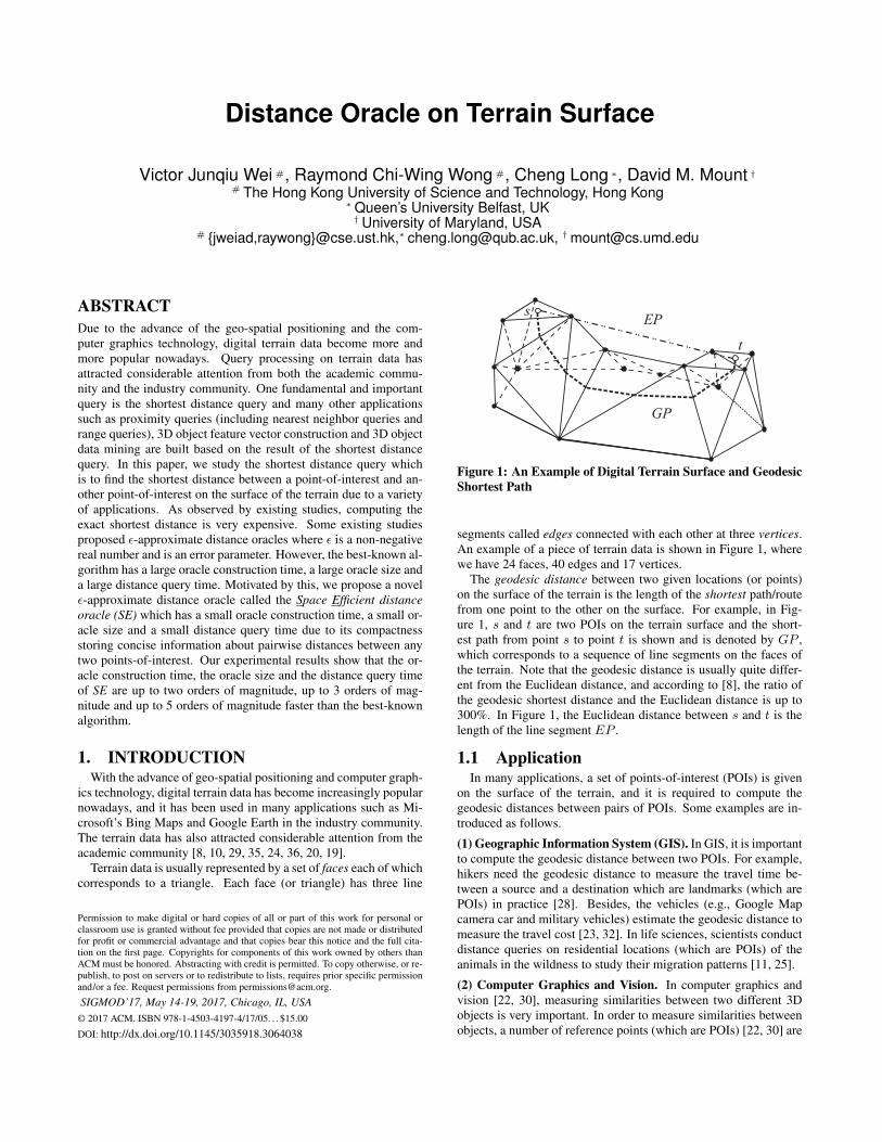
Figure 1: An Example of Digital Terrain Surface and GeodesicShortest Path

segments called edges connected with each other at three vertices.An example of a piece of terrain data is shown in Figure 1, wherewe have 24 faces, 40 edges and 17 vertices.

The geodesic distance between two given locations (or points)on the surface of the terrain is the length of the shortest path/routefrom one point to the other on the surface. For example, in Fig-ure 1, s and t are two POIs on the terrain surface and the short-est path from point s to point t is shown and is denoted by GP ,which corresponds to a sequence of line segments on the faces ofthe terrain. Note that the geodesic distance is usually quite differ-ent from the Euclidean distance, and according to [8], the ratio ofthe geodesic shortest distance and the Euclidean distance is up to300%. In Figure 1, the Euclidean distance between s and t is thelength of the line segment EP .

1.1 ApplicationIn many applications, a set of points-of-interest (POIs) is given

on the surface of the terrain, and it is required to compute thegeodesic distances between pairs of POIs. Some examples are in-troduced as follows.

(1) Geographic Information System (GIS). In GIS, it is importantto compute the geodesic distance between two POIs. For example,hikers need the geodesic distance to measure the travel time be-tween a source and a destination which are landmarks (which arePOIs) in practice [28]. Besides, the vehicles (e.g., Google Mapcamera car and military vehicles) estimate the geodesic distance tomeasure the travel cost [23, 32]. In life sciences, scientists conductdistance queries on residential locations (which are POIs) of theanimals in the wildness to study their migration patterns [11, 25].

(2) Computer Graphics and Vision. In computer graphics andvision [22, 30], measuring similarities between two different 3Dobjects is very important. In order to measure similarities betweenobjects, a number of reference points (which are POIs) [22, 30] are

selected on the surface of each object. These reference points playan important role in similarity measurement since they are invari-ant to transformations such as rotation and translation. For eachobject, geodesic distances between all pairs of reference points arecomputed and are stored as a feature vector for similarity measure-ment. In this application, multiple geodesic distance computationsare involved.(3) Scientific Data 3D Modeling. There is a need to model scien-tific data in 3D models in areas like biology, chemistry, anthropol-ogy and archeology [1, 17]. In neuroimaging, similar to computergraphics and vision, a 3D model of an organ is associated with aset of reference points [1, 17] (which are POIs) and these referencepoints correspond to functional units on the organ and the scientistsuse the geodesic distance between reference points to analyze tu-mor development with magnetic resonance imaging (MRI) images.In neuroscience, scientists conducted spatial queries on a 3D brainmodel to study the neuron density and the number of branches ina region of the brain [31]. Similarly, multiple geodesic distancecomputations are involved in this application.(4) Online 3D Virtual Game. In some online 3D virtual gameslike INGRESS, a city (e.g., San Francisco in game INGRESS) hasa terrain surface which consists of a number of portals (which arePOIs). For each portal, it is important to calculate the geodesicdistance from this portal to each of the other portals so that theinfluence of this portal is estimated. Here, multiple computationsfor geodesic distances are involved.(5) Spatial Data Mining. There are many data mining techniquesused in the spatial databases. For example, in the clustering tech-nique, the inner-cluster distance and the inter-cluster distance areneeded. In the co-location pattern mining, shortest distance queries,are also used frequently. In a city, buildings and parks can be POIsand in the wildness, radio-telemetry receivers set up for collect-ing animal movement data could be POIs. In the context of spatialdata mining, the number of geodesic distance computations is verylarge.

1.2 MotivationConsider a terrain T with N vertices. Let P be a set of n POIs

on the surface of the terrain.Due to a variety of applications in different domains as described

in Section 1.1, computing geodesic distances [26, 6, 34, 24, 20,19, 2, 3, 12] is very important and is very fundamental to otherproximity queries such as nearest neighbor queries [9, 10, 29, 35,20, 19], range queries [20, 19] and reverse nearest neighbor queries[36, 20].

Motivated by this, we aim to study three kinds of queries, namelyvertex-to-vertex (V2V) distance queries, POI-to-POI (P2P) dis-tance queries and arbitrary point-to-arbitrary point (A2A) distancequeries. Consider the first two types of queries. Each V2V distancequery returns the geodesic distance between a starting point s and adestination point t, where both s and t are vertices (from V ). EachP2P distance query returns the geodesic distance between a startingpoint s and a destination point t, where both s and t are POIs (fromP ). Since P2P distance queries, considering both the concept ofvertices and the concept of POIs, is more general than V2V dis-tance queries, considering only the concept of vertices without theconcept of POIs, P2P distance queries could be regarded as a gener-alization of V2V distance queries. Specifically, under the problemsetting for P2P distance queries, if for each vertex in the problemsetting for V2V distance queries, we create a POI which has thesame coordinate values as this vertex, then the P2P distance querieswill become the V2V distance queries. Thus, for clarity, in this pa-per, we focus on P2P distance queries. Consider the third type of

queries. Each A2A distance query returns the geodesic distance be-tween a starting point s and a destination point t, where both s andt are two arbitrary points on the surface of the terrain. Since A2Adistance queries allow all possible points on the surface of the ter-rain, A2A distance queries generalize both P2P and V2V distancequeries. For the ease of illustration, in the main body of this paper,we first study P2P distance queries. Later, in Appendix C, we studyA2A distance queries.

Our natural goal of answering each P2P distance query is to re-turn the corresponding distance in a short time. However, none ofthe existing studies [26, 6, 34, 24, 20, 19, 2, 3, 12] could achievethis goal satisfactorily.

Firstly, all existing algorithms [26, 6, 34] computing exactgeodesic distances on-the-fly are still slow even in the moderate-sized terrain data. The time complexities of the algorithms forcomputing exact geodesic distances proposed by [26, 6, 34], areO(N2 logN), O(N2), O(N log2N) and O(N2 logN), respec-tively, which is still very large whenN is large. In the literature [29,35, 20, 19], the algorithm proposed in [6] is recognized as a state-of-the-art fastest algorithm. Many existing papers [29, 35, 20, 19]adopt this for finding the geodesic distance. According to [19], thealgorithm proposed in [6] took more than 300 seconds on a terrainwith 200K vertices, which is very slow.

Secondly, although some existing algorithms [24, 20, 19] wereproposed to compute approximate geodesic distances on-the-fly forreducing the computation time, all of these algorithms are still notefficient enough for proximity queries and applications involvingmany distance queries. The algorithm in [24] computes the approx-imate geodesic distance/path satisfying a slope condition, the algo-rithm in [20] computes the lower and upper bounds of the geodesicdistances between two points, and it provides no guarantees on thequalities of the bounds found, and the algorithm in [19], which is animproved version of that in [20], runs inO((N+N ′) log(N+N ′))time where N ′ is the number of additional vertices introduced forthe sake of the guarantee on the qualities of the lower and upperbounds found.

1.3 Distance OracleMotivated by these, to efficiently process the geodesic distance

queries, especially for those cases where queries for many differ-ent pairs of points are issued, some existing studies [2, 3, 12] aimat designing geodesic distance (and/or the corresponding shortestpath) oracles. To the best of our knowledge, all existing studies fo-cused on building oracles for returning approximate geodesic dis-tances only but no existing studies focused on building oracles forreturning exact geodesic distances (which could be explained bythe high computation cost of computing the exact geodesic dis-tances). All of these studies [2, 3, 12] are based on auxiliarypoint-based oracles. Specifically, they first introduce a large num-ber of auxiliary points (edges), namely Steiner points (edges), onthe surface of the terrain where each Steiner edge connects twoSteiner points. Then, they construct a graph Gε whose vertices(edges) are either original vertices (edges) or the Steiner points(edges). The exact distance between any two vertices/points onGε is an ε-approximate geodesic distance between these two ver-tices/points. The ε-approximate geodesic distance oracles proposedin [2, 3, 12] indexes the exact distances on Gε. Among these stud-ies, the oracle in [12] is the best, where the space complexity ofthe oracle (called the oracle size) is O( N

sin(θ)·ε1.5 log2(Nε

) log2 1ε)

where θ is the minimum inner angle of any face of the terrainsurface. It can answer ε-approximate P2P distance queries inO( 1

sin(θ)·ε log 1ε

+ log logN) time.Unfortunately, these auxiliary point-based oracles have two

drawbacks. The first drawback is that each of these oracles hasa large oracle building time and a large oracle size. This is becausea large number of Steiner points (edges) are introduced during theoracle construction and the number of Steiner points could be sev-eral orders of magnitude larger than the number of vertices on thesurface of the terrain. Thus, each of these oracles has a poor em-pirical performance in terms of both the oracle building time andthe oracle size. The second drawback is that each of these oraclesis constructed based on the structure of the terrain without consid-ering the information about POIs. In other words, it is constructedbased on the set of vertices regardless of the set of POIs. For ex-ample, consider the case where there are only two POIs, a naiveoracle storing the geodesic distance for one pair (of POIs) occupiesaO(1) space only but the oracle in [12] could introduce millions ofSteiner points, resulting in a large oracle size and a large buildingtime.

Motivated by the drawbacks of the existing methods, we pro-pose a distance oracle called the Space-Efficient Distance Oracle(SE) such that for any point s and any point t in P , the oracle re-turns an ε-approximation of the geodesic distance between s and tefficiently, where ε is a non-negative real user parameter, called theerror parameter. Our SE has three good features: (1) low construc-tion time, (2) small size and (3) low query time (compared with thebest-known oracle [12]). This is because SE is space-efficient inthe sense that its size is linear to n (i.e., no of POIs). Due to thisspace-efficient property, it is much easier for us to design an effi-cient algorithm for constructing the SE and an efficient algorithmfor answering distance queries.

1.4 Contribution & OrganizationWe summarize our major contributions as follows. Firstly, we

propose a novel distance oracle called SE, which can be computedefficiently, has small size and can answer ε-approximate geodesicdistance queries efficiently. Secondly, our SE answers not onlyP2P distance queries but also V2V distance queries. Thirdly, inV2V distance queries, our experimental results show that the build-ing time, oracle size and query time of SE are, respectively, 5-100times, 10-100 times and more than 1000 times smaller than thoseof the best-known distance oracle [12] on benchmark real datasets.In P2P distance queries, the building time, oracle size and querytime of SE are 10-100 times, 10-1000 times and 100-10000 timessmaller than those of the best-known distance oracle [12] on bench-mark real datasets, respectively.

The remainder of the paper is organized as follows. Section 2provides the problem definition. Section 3 presents our distance or-acle, namely SE. Section 4 reviews the related work and introducessome baseline methods. Section 5 presents the experimental resultsand Section 6 concludes the paper.

2. PROBLEM DEFINITIONConsider a terrain T . Let V be the set of all vertices on the

surface of the terrain T , andE be the set of all edges on the surfaceof the terrain T . Let N be the size of T (i.e., N = |V |). Eachvertex v ∈ V has three coordinate values, denoted by xv, yv andzv .

Let P be a set of POIs on the surface of the terrain T and n be thesize of P (i.e., n = |P |). In the following discussion, we focus onthe case when n ≤ N . This is because in real-life applications, n ≤N . For example, in the BearHead dataset, one benchmark datasetused in the literature, n = 4k and N = 1.4M . In the EaglePeakdataset, the other benchmark dataset, n = 4k and N = 1.5M .The discussion about how we handle the case when n > N can befound in Appendix D. Each POI p ∈ P also has three coordinate

values, denoted by xp, yp and zp. In this paper, we assume thatP contains no duplicate points since any two co-located POIs canbe regarded as one POI in practice, and we can merge any two co-located POIs into one POI by a simple preprocessing step.

Given two points, s and t, on the surface of T , the geodesicshortest path between s and t, denoted by Πg(s, t), is defined tobe the shortest path between the two points on the surface of T .Note that the geodesic shortest path corresponds to a sequence ofline segments on the surface of the terrain. Consider the examplein Figure 1 where the geodesic shortest path between two points sand t is denoted by GP . Given two points, s and t, on the surfaceof T , the geodesic distance between s and t, denoted by dg(s, t),is defined to be the length of the geodesic shortest path betweenthe two points, i.e., Πg(s, t), where the length of a path is definedto be the sum of the lengths of all line segments of the path. Thegeodesic distance dg(·, ·) is a metric, and therefore it satisfies thetriangle inequality.

Note that a full materialization of geodesic distances for all pos-sible pairs of points in P is not feasible since the complexity ofthe oracle size and the complexity of the oracle building time areO(n2) and O(nN log2N), respectively, which are prohibitivelylarge.

3. DISTANCE ORACLEWe first present the overview of our distance oracle called SE in

Section 3.1. Then, we present the first component of SE, called thecompressed partition tree, in Section 3.2, the second componentof SE, called the node pair set, in Section 3.3, the query processingalgorithm based on SE in Section 3.4, the construction algorithm ofSE in Section 3.5, and some theoretical results of SE in Section 3.6.

3.1 OverviewBefore giving an overview, we first give the concept of a

disk. Given a point p ∈ P and a non-negative real numberr, a disk centered at p with radius equal to r on the terrainsurface, denoted by D(p, r), is defined to be a set of all pos-sible points on the terrain surface whose geodesic shortest dis-tance to p is at most r. That is, D(p, r) = {p′|dg(p′, p) ≤r and p′ is an arbitrary point on the terrain surface}.

With this concept, we are ready to describe our distance oracleSE which includes two major components, namely the compressedpartition tree and the node pair set.

The first component is the compressed partition tree in whicheach node corresponds to a disk containing a set of POIs. In theleaf level of the tree, there are n nodes each of which correspondsto a disk containing only one POI. Each node in this level has thesmallest radius (since each node contains only one POI). In thelevel just above the leaf level of the tree, there are fewer nodes eachof which corresponds to a disk containing one or more POIs. Eachnode in this level has a larger radius (since each node contains oneor more POIs). Similarly, each node in a higher level has a largerradius. At the root level of the tree, the (root) node has the largestradius since it contains all n POIs. Note that for different levels,the tree has different number of nodes (with different radius).

The second component is the node pair set which is a set of thepairs of nodes from the compressed partition tree. In this node pairset, each node pair in the form of 〈O,O′〉 is associated with thedistance between the centers of the corresponding disks of O andO′ where O and O′ are two nodes in the compressed partition tree.Besides, the node pair set satisfies one interesting property calledthe unique node pair match property which is the key to the queryefficiency of our SE. The unique node pair match property statesthat for any two points, namely p and q, in P , there exists exactly

one node pair 〈O,O′〉 in the node pair set such that O contains pand O′ contains q.

Consider a distance query with a source point s ∈ P and a des-tination point t ∈ P . Let h be the height of the tree. In all ofour experimental results on benchmark real terrain datasets, h issmaller than 30. We could answer this distance query in O(h) timeusing SE. The major idea is to find a node pair 〈O,O′〉 in the nodepair set efficiently such that O contains s and O′ contains t, and re-turn the distance associated with this node pair. Interestingly, eventhough the distance returned is associated to this node pair, it willbe shown later that the distance returned is an ε-approximation ofthe geodesic distance between s and t.

The major challenge here is how to design SE which achieves thespace-efficient property (mentioned in Section 1). We will describethe details of how we address this challenge.

3.2 Oracle Component 1: Compressed Parti-tion Tree

In this section, we first present a hierarchical structure called apartition tree to index all POIs in P , which is used for construct-ing the first component (i.e., the compressed partition tree) of ourdistance oracle SE.

A partition tree is defined to be a tree with the following compo-nents.• Each nodeO in the tree has two attributes, namely its center,

denoted by cO , and its radius, denoted by rO , where cO is apoint in P and rO is a non-negative real number.• For each leaf node O, D(cO, rO) contains only one point inP (which is cO) (and thus contains no objects in P other thancO). Note that there are n leaf nodes.• For each internal node O, the center of each child of nodeO is in D(cO, rO) and the radius of each child of node O isequal to 0.5 · rO .• Each node O in the tree is associated with its representative

set, denoted by RS(O), which is defined to be a set contain-ing the centers of all the leaf nodes in the subtree rooted atO.

Given two nodes, namely O and O′, the (geodesic) distancebetween O and O′, denoted by dg(O,O

′), is defined to bedg(cO, cO′).

Let h be the height of the partition tree. The partition tree hash + 1 layers, namely Layer 0, Layer 1, ..., Layer h. Layer 0 is thelayer containing the root node only. For each i ∈ [1, h], Layer i isthe layer containing all child nodes of each node in Layer (i − 1).Finally, Layer h is the layer containing all leaf nodes. If a node isin Layer i where i ∈ [0, h], we also say that the depth of this nodeis i. Note that all nodes in the same layer have the same radii. Theradius of Layer i, denoted by ri, is defined to be the radius of oneof the nodes in Layer i. For any i, j ∈ [0, h], we say that Layer i ishigher than Layer j (or Layer j is lower than Layer i) if and onlyif i < j.

Next, we give the three properties of this partition tree to be sat-isfied. We will describe how to construct a partition tree satisfyingthese three properties later.• Separation Property: For each i ∈ [0, h], the radius of each

node in Layer i is r02i

and the geodesic distance between anytwo nodes in this layer is at least r0

2i.

• Covering Property: For each layer where X denotes aset of all nodes in this layer, the region represented by⋃O∈X D(cO, rO) covers all points in P .

• Distance Property: For each nodeO in the tree, ifO′ is oneof the descendant nodes of O, then dg(cO, cO′) is at most2 · rO , i.e., cO′ is in the disk D(cO, 2 · rO).

Given a node O in the partition tree, the enlarged disk of nodeO is defined to be D(cO, 2 · rO). From the Distance Property,we deduce that for each node O in the partition tree, all points inRS(O) (which are points in P ) are in the enlarged disk of node O.

EXAMPLE 1 (PARTITION TREE). Consider the points on aterrain surface as shown in Figure 2. There are 12 pointsp1, p2, p3, ......, p12 in P .

Figure 3 shows three small disks, namely D(p1, r3), D(p2, r3)and D(p3, r3), one medium-small disk, namely D(p2, r2), onemedium-large disk, namely D(p2, r1), and one large disk, namelyD(p7, r0), where r0, r1, r2 and r3 are four non-negative real num-bers. Note that r0 is the radius of the large disk, r1 is the radius ofthe medium-large disk, r2 is the radius of the medium-small diskand r3 is the radius of one of the small disks. We also show alldisks to be used in this example in Figure 4.

There are 21 disks in the figure, each of which centers at a point.For example, the disk D(p7, r0) is a disk with its center equal top7 and its radius equal to r0 = dg(p7, p11).

Figure 5 shows a partition tree of height equal to 3 which isbuilt based on the 12 points shown in Figure 2. In this figure, eachblack dot corresponds to a node in the tree. By definition, any twonodes in the same layer have the same radii. In Layer 0, there isonly one node O21 (i.e., the root node) with its radius r0 equal todg(p7, p11). In Layer 1, there are three nodes, namely O18, O19

and O20, each with its radius r1 equal to 0.5r0. In Layer 2, thereare 5 nodes, namely O13, O14, O15, O16 and O17 each with its ra-dius r2 equal to 0.25r0. In Layer 3, there are 12 nodes (i.e., leafnodes), namely O1, O2, ..., O12, each with its radius r3 equal to0.125r0. In the figure, we list the center of each node below thelabel of the node. For example, there is a label p2 below the labelO13, which means that the center of O13 is p2.

Consider the leaf node O1 with its center equal to p1 and itsradius equal to r3. It is easy to see that diskD(p1, r3) contains onlyone point in P (i.e., p1) as shown in Figure 3. The representativeset of this node is a set containing only the center of this node (i.e.,p1). This holds as well for each of the other leaf nodes (e.g., nodeO2 and node O3).

Consider the internal node O13 with its center equal to p2 andits radius equal to r2. The center of each child of node O13 (i.e.,node O1, node O2 and node O3) is in disk D(p2, r2) as shown inFigure 3. Besides, the radius of each child of node O13 is equalto 0.5 · r2 (since the radius of each child is equal to 0.125r0 andr2 = 0.25r0). The representative set of this node is a set containingthe centers of all the leaf nodes in the subtree root at O13 (i.e., thecenter of node O1 (which is p1), the center of node O2 (which isp2) and the center of nodeO3 (which is p3)). This holds as well foreach of the other internal nodes.

It is easy to verify that the partition tree shown in this figuresatisfies the three properties described above.

Next, we present our top-down method for building the partitiontree.• Step 1 (Root Node Construction): We create the root node as

follows.– Step (a) (Initialization): We assign a variable i, denoting

the layer number, with 0.– Step (b) (Point Selection): We randomly select a point p in

P .– Step (c) (Radius Computation): We perform a single-

source all-destination (SSAD) exact shortest path algo-rithm [34, 6, 26] which takes p as an input of the sourcepoint and executes until the search region of the algo-rithm covers all points in P . When we terminate the

p10

p9

p8

p7

p6

p5

p4

p3

p2

p1

p12

p11

Figure 2: An Example

D p ,r( )2 2

p10

p9

p8

p7

p6p

5

p4

p3

p2

p1

p12

p11

D p ,r( )3 3

D p ,r( )1 3

D p ,r( )7 0

r =0.5r1 0

1r =0.5r

2

2r =0.5r

3

D p ,r( )2 1

D p ,r( )2 3

Figure 3: Some Disks Used in Our Example

p10

p9

p8

p7

p6p

5

p4

p3

p2

p1

p12

p11

D p ,r( )2 2

D p ,r( )7 0

r =0.5r1 0

1r =0.5r

2

2r =0.5r

3

D p ,r( )2 1

D p ,r( )5 2

D p ,r( )7 1

D p ,r( )10 1

D p ,r( )10 2

D p ,r( )12 2

D p ,r( )7 2

Figure 4: All Disks Used in Our Example

Layer 0:

Layer 1:

Layer 2:

Layer 3:

r r2 0=0.25

r =60

r r3 0=0.125

r1=0.5r

0

O1

O12

O11

O10O

9O8

O7

O6

O5

O4

O3

O2

O21

O18 O

19O

20

O17

O16

O15

O14O

13

p7

p7

p2

p12p

10p7

p5

p2

p12

p11

p10

p9

p8

p7p

6p

5p

4p

3p

2p

1

p10

Figure 5: An Example of Partition Tree

Layer 0:

Layer 1:

Layer 2:

Layer 3:

r r2 0=0.25

r =60

r3=0

r1=0.5r

0

O1

O12

O11

O10O

9O8

O7

O6

O5

O4

O3

O2

O21

O19 O

20

O16

O15

O14O

13

p12

p11

p10

p9

p8

p7p

6p

5p

4p

3p

2p

1

p10p

7p

5p

2

p7

p7

p10

Figure 6: An Example of Compressed Par-tition Tree

Layer 0:

Layer 1:

Layer 2:

Layer 3:

r r2 0=0.25

r =60

r3=0

r1=0.5r0

O O10 t( )O O1 s( )

O21

O20

O16O13

As At

O21 O21

O20

O13 O16

O1O10

Figure 7: An Example of DistanceQuery Processing

algorithm, we obtain the maximum distance d betweenp and a point in P .

– Step (d) (Node Construction): We create a root node Owhere its center is set to p and its radius is set to d.Note that in this layer, r0 = d.

• Step 2 (Non-Root Node Construction): We perform the follow-ing operations.

– Step (a) (Initialization): We increment variable i by 1. Weassign a variable P ′, denoting a set of remaining pointsin P to be “covered” by a node in Layer i, with P .

– Step (b) (Iterative Step): We perform the following itera-tive steps.

∗ Step(i) (Point Selection): Let C be a set containing thecenters of all nodes in Layer i − 1 and let PC bethe set of remaining points in P ′ each of which isone of the centers of all nodes in Layer i− 1 (i.e.,PC = P ′ ∩ C). We randomly select a point p fromPC if PC 6= ∅, and select a point p from P ′ basedon a point selection strategy (to be described later)otherwise.

∗ Step (ii) (Point Covering): We find a set S of all pointsin P ′ that are in D(p, r0

2i) by performing a single-

source all-destination (SSAD) exact shortest pathalgorithm which takes p as an input of the sourcepoint and executes the algorithm until the distancebetween the boundary of the search region and pis greater than r0

2i. We remove all points in S from

P ′.∗ Step (iii) (Node Creation): We create a node O where

its center is set to p and its radius is set to r02i

. Then,we find the node Oparent in Layer (i − 1) whosedistance to O is the minimum. We set the parentof O to Oparent .

∗ Step (iv) (Additional Node Creation): We repeat theabove steps (i.e., Steps (i)-(iii)) until P ′ is empty.

– Step (c) (Next Layer Processing): We repeat the abovesteps (i.e., Step (a) and Step (b)) until the number ofnodes in Layer i is equal to n.

LEMMA 1. The partition tree generated by the above proceduresatisfies the Separation, Covering and Distance Properties.

PROOF. For the sake of space, all the proofs in the paper can befound in Appendix B.

Some implementation details of this algorithm are given as fol-lows.Implementation Detail 1 (Point Selection Strategy in Step2(b)(i)): We propose two heuristic-based point selection strategiesas follows. The first one is called the random selection strategy.It randomly selects a point p from P ′. The second one is calledthe greedy selection strategy which is to select a point from P ′ inthe “densest” region (or formally cell) on the surface of the terrain.The major idea of this strategy is to select a point from P ′ in thedensest region (because if this point is selected as the “center” ofthe disk, then this disk can cover many points (which could comefrom the densest region)). Specifically, this strategy requires someadditional operations included in other steps, and we describe themas follows. (A) Between Step 2(a) and Step 2(b), we construct agrid on the x-y plane with the cell width equal to O( r0

2i). Then, we

insert all points from P ′ in corresponding cells, and all point IDsin each cell are indexed in a B+-tree. We also build a max-heapcontaining all non-empty cells whose keys are the sizes of theirB+-trees. (B) In Step 2(b)(i), in the case that PC = ∅, we select apoint p in P ′ by finding the cell with the greatest number of pointsin P ′ and randomly selecting a point p from P ′ in the cell. (C) InStep 2(b)(ii), for each point p′ in S, we remove p′ from the B+-tree of its corresponding cell and decrease the key of the cell in themax-heap by 1.Implementation Detail 2 (SSAD algorithm): Note that in Step1(c) and Step 2(b)(ii), we need to perform the SSAD algorithm [6,

26] which is a best-first search algorithm. There are two versions ofthis algorithm here, but the major principle is the same for each butwith different stopping criteria. The major principle is describedas follows. The algorithm performs a search that starts from s andexpands its search with the vertex in V which has not been pro-cessed and has its minimum geodesic distance dmin to s. For eachvertex expansion, all points in P on each face expanded togetherwith the vertex are computed with their geodesic distances. Notethat we know that for each vertex expansion, all vertices in V withtheir geodesic distances smaller than dmin have been processed.The first version of this algorithm (in Step 1(c)) has an input of asource point s only. For each vertex expansion, the first versionof the algorithm checks whether all points in P have been visited.If yes, this algorithm terminates. The second version of this algo-rithm (in Step 2(b)(ii)) takes as its inputs a source point s and adistance threshold d′ (denoting the boundary of the search regionstarting from s). For each vertex expansion, the second version ofthe algorithm checks whether dmin is larger than d′. If yes, thisalgorithm terminates. The time complexity of each of these twoversions is O(N logN + k), whereN is the number of vertices inV processed and k is the number of points in P processed.

Finally, we analyze the depth h of the partition tree. The follow-ing lemma presents the depth of the partition tree.

LEMMA 2. h ≤ log(maxp,q∈P dg(p,q)minp,q∈P dg(p,q)

) + 1

By our assumption of Section 2 that there are no duplicate POIs,it follows that minp,q∈P dg(p, q) is strictly positive. We want toemphasize that the upper bound of h (i.e., log(

maxp,q∈P dg(p,q)minp,q∈P dg(p,q)

) +

1) is a small value in practice. Firstly, in all of our experimentalresults, h is at most 30. Secondly, even in the extreme case wherethe minimum distance is one nanometer (= 10−9m) and the max-imum distance is the length of the Earth’s equator (≈ 4 × 107m),Lemma 2 yields an upper bound of only 56.

Consider the first component called the compressed partition treewhich is a variation of the partition tree.

We construct the compressed partition tree Tcompress based onthe original partition tree Torg as follows. Firstly, we generateTcompress by duplicating Torg . Secondly, whenever there is a nodeO in Tcompress containing only one child node Ochild , if there is aparent node Oparent of O, then we remove the parent-and-child re-lationship betweenO andOchild and then the parent ofOchild is setto Oparent . Then, we delete O. We repeat this step iteratively untilthere is no node in Tcompress containing only one child. Thirdly, foreach leaf node in Tcompress , we set its radius to 0.

Note that each leaf node (containing no child node) is still keptafter the above operation since each node removal operation in-volves a node containing only one child node. Note that for eachpoint p in P , there exists exactly one leaf node whose center is p.Given a point p in P , its corresponding leaf node, denoted byOp, isdefined to be the leaf node in the compressed partition tree whosecenter is p. Besides, given a node O in the compressed partitiontree, the layer number of the layer containing O in the compressedpartition tree is defined to be the layer number of the layer contain-ing O in the (original) partition tree.

EXAMPLE 2 (COMPRESSED PARTITION TREE). Considerthe partition tree (Figure 5) in Example 1. According to the aboveprocedure, since node O17 has only one child node (i.e., nodeO12), we remove the parent-and-child relationship between O17

and O12 and then we set the parent of O12 to node O20 (which isthe parent of O17 in the original partition tree). Then, we removenode O17. After this operation, we do a similar operation for node

O18 containing only one child node O13. After that, no node in theresulting tree contains only one child. Finally, for each leaf node inthe resulting tree, we set its radius (i.e., r3) to 0. The resulting treeis the compressed partition tree as shown in Figure 6. Note that thelayer number of the layer containing node O20 is 1 and the layernumber of the layer containing node O12 is 3 (although the nodeO17 in Layer 2 of the (original) partition tree (which connects O12

and O20) is removed).

As will be shown later, the space complexity of the compressedpartition tree is O(n) (which is linear to n).

3.3 Oracle Component 2: Node Pair SetConsider the second component of SE called the node pair set.

Before we define this, we give some definitions based on the com-pressed partition tree which will be used in the node pair set.

Given two nodes O and O′ in the compressed partition tree, Oand O′ are well-separated [5] if and only if dg(cO, cO′) ≥ ( 2

ε+

2) ·max{r, r′} where r is the radius of the enlarged disk of O andr′ is the radius of the enlarged disk of O′. Given two nodes O andO′ which are well-separated in the compressed partition tree, wesay that 〈O,O′〉 is a well-separated (node) pair.

Given a node pair 〈O,O′〉 and two nodes O and O′ in a treewhere (1) O is either O or a descendant node of O and (2) O′ iseither O′ or a descendant node of O′, we say that 〈O,O′〉 contains〈O,O′〉. Note that in our context, a node pair 〈O,O′〉 has an order.Specifically, even if 〈O,O′〉 contains 〈O,O′〉, it is possible that〈O′, O〉 does not contain 〈O,O′〉.

In practice, given two points p and q ∈ P with their correspond-ing leaf nodes Op and Oq in the compressed partition tree, we saythat 〈O,O′〉 contains 〈p, q〉 if 〈O,O′〉 contains 〈Op, Oq〉.

Next, we give a method of generating the node pair set given acompressed partition tree. We maintain a variable S storing a set ofnode pairs, initialized as {〈Oroot , Oroot〉} where Oroot is the rootnode of the compressed partition tree. At each iteration, we extracta pair 〈Oi, Oj〉 from S which is not well-separated. Then, we selectthe node in the pair 〈Oi, Oj〉whose radius is larger. Without loss ofgenerality, we assume that Oi is selected and let C1, C2, ......, Cmdenote its children. Next, we insert 〈C1, Oj〉, 〈C2, Oj〉, ..., and〈Cm, Oj〉 into S. For each x ∈ [1,m], 〈Cx, Oj〉 is said to be apair generated by 〈Oi, Oj〉 andOi is said to be split from 〈Oi, Oj〉.Note that if Oi and Oj have the same radius, then we select thenode with a smaller node ID in the pair 〈Oi, Oj〉 for processing. Werepeat the above procedure until each pair in S is well-separated.

Let S be the set of node pairs returned by the above procedure.S is called the node pair set of SE.

In the above procedure, note that whenever we check whethera node pair 〈Oi, Oj〉 is well-separated, we have to compute thedistance between Oi and Oj . Later in Section 3.5 as a part of theoracle construction, we will explain how we compute this distanceefficiently.

The following theorem shows a key property of the node pair setgenerated, namely the unique node pair match property.

THEOREM 1. Let S be the node pair set of SE. Each node pairin S is a well-separated pair and for any two points p and q in P ,there exists exactly one node pair 〈O,O′〉 in S containing 〈p, q〉and the distance associated with this node pair is an ε-approximatedistance of dg(p, q).

Next, we present the following theorem showing that there areO( nh

ε2β) node pairs considered in the procedure of generating the

node pair set (which is linear to n) where β is a real number and isin the range from 1.5 and 2 in practice.

THEOREM 2. There are only O( nhε2β

) node pairs considered inthe procedure of generating the node pair set and thus there areO( nh

ε2β) in the node pair set of SE.

Finally, we adopt a standard hashing technique, namely the per-fect hashing scheme [7], to index all node pairs in the node pair setof SE. The hashing technique takes a linear space and requires alinear preprocessing time in expectation in terms of the number ofthe node pairs in the node pair set of SE. Given two nodes O andO′ in the compressed partition tree, we could check whether thereexists a node pair 〈O,O′〉 in the node pair set of SE in constanttime and if so, it could also return the associated geodesic distancedg(O,O

′) in constant time.

3.4 Query ProcessingNext, we present how we use our distance oracle SE for a dis-

tance query with a source point s ∈ P and a destination pointt ∈ P .

We first present one naive method, whose time complexity isO(h2), for this distance query. Next, we present an efficient algo-rithm whose time complexity is O(h).Naive Method: Before we introduce the naive method, we givesome notations first. Let Oroot be the root node of the compressedpartition tree. By our notation convention, we know that Os de-notes the corresponding leaf node of point s in the compressed par-tition tree and Ot denotes the corresponding leaf node of point t inthe compressed partition tree. Let As be the array of size h + 1where As[i] is equal to the node in Layer i along the path from Osto Oroot in the compressed partition tree if there exists a node inLayer i and is equal to ∅ otherwise for each i ∈ [0, h]. We have an-other notation At which has a definition similar to As and involvesthe path starting from Ot instead of Os. We denote the Cartesianproduct between the set of all nodes in As and the set of all nodesinAt byAs×At. It is easy to have the following observation fromTheorem 1: there exists exactly one pair 〈O,O′〉 in As × At suchthat 〈O,O′〉 contains 〈s, t〉 and 〈O,O′〉 is in the node pair set ofour SE.

Based on this observation, we have the following naive methodfor a distance query. Firstly, we find a leaf node Os and a leafnode Ot. Then, we construct array As (At) by traversing from Os(Ot) to Oroot . Secondly, for each node O ∈ As and each nodeO′ ∈ At, we check whether node pair 〈O,O′〉 is in the node pairset of our SE. If so, we return the distance associated with 〈O,O′〉.Otherwise, we continue to check the next node pair.

Note that by this observation, the above naive method must re-turn one distance value (associated with one node pair) at the end.

The correctness of the naive method (i.e., the ε-approximation)comes naturally from Theorem 1.

It is easy to verify that the time complexity of the naive methodis O(h2) since the first step takes O(h) time and the second steptakes O(h2) time (because the second step involves O(h2) nodepairs and each node pair requires to be checked with its existencein the node pair set of our SE inO(1) time using the perfect hashingscheme).Efficient Method: Next, we will present our efficient algorithm forthe distance query which takes O(h) time. Before we present thealgorithm, we give some concepts first.

Let Layer(O) be the layer number of the layer containing nodeO.

We categorize node pairs 〈O,O′〉 into one of three types. Anode pair 〈O,O′〉 is said to be a same-layer node pair if Ohas the same layer as O′ in the compressed partition tree (i.e.,Layer(O) = Layer(O′)). A node pair 〈O,O′〉 is said to be

a first-higher-layer node pair if O has a higher layer than O′ inthe compressed partition tree (i.e., Layer(O) < Layer(O′)). Anode pair 〈O,O′〉 is said to be a first-lower-layer node pair if Ohas a lower layer than O′ in the compressed partition tree (i.e.,Layer(O) > Layer(O′)).

Consider the compressed partition tree as shown in Figure 6.The node pair 〈O14, O15〉 is a same-layer node pair. The nodepair 〈O14, O7〉 is a first-higher-layer node pair and the node pair〈O6, O15〉 is a first-lower-layer node pair.

By definition, in a same-layer node pair 〈O,O′〉, both node Oand node O′ are in the same layer. We know that in a first-higher-layer node pair 〈O,O′〉, since node O has a higher layer than nodeO′, we know that there exists a layer higher than the layer contain-ing node O′, and thus we deduce that O′ has a parent node in thecompressed partition tree. With the following lemma, interestingly,we know that the layer containing the parent of node O′ is equal toor higher than the layer containing nodeO. We could have a similarconclusion for a first-lower node pair.

LEMMA 3. Consider a node pair 〈O,O′〉 in the node pair setof our SE. If 〈O,O′〉 is a first-higher-layer node pair, then the layercontaining the parent of nodeO′ is equal to or higher than the layercontaining node O. If 〈O,O′〉 is a first-lower-layer node pair, thenthe layer containing the parent of nodeO is equal to or higher thanthe layer containing node O′.

Consider the compressed partition tree as shown in Figure 6.The error parameter ε is set to 2. Note that for illustration pur-pose, this error parameter is set to 2 but in practice, it should beset to a smaller value (e.g., 0.1) as what we did in our experimentalstudies. The node pairs 〈O14, O7〉 and 〈O16, O12〉 are both first-higher-layer node pairs in the node pair set of our SE. The parentof O7 (O12) is O15 (O20). The layer containing O15 is the sameas that containing O14 and the layer containing O20 is higher thanthat containing O16. Similar illustrations could be made to the twofirst-lower-layer node pairs in the node pair set of our SE, namely〈O6, O15〉 and 〈O13, O20〉, in a symmetric way.

Let parent(O) be the parent of node O in the compressed par-tition tree.

With Lemma 3, we have the following observation.

OBSERVATION 1. Consider a node pair 〈O,O′〉 in the nodepair set of our SE. If 〈O,O′〉 is a first-higher-layer node pair, thenLayer(parent(O′)) ≤ Layer(O) < Layer(O′). If 〈O,O′〉is a first-lower-layer node pair, then Layer(parent(O)) ≤Layer(O′) < Layer(O).

Consider the compressed partition tree as shown in Fig-ure 6. The node pairs 〈O14, O7〉 and 〈O16, O12〉 are bothfirst-higher-layer node pairs in the node pair set of our SE.parent(O7) (parent(O12)) is O15 (O20). It is clear thatLayer(parent(O7)) ≤ Layer(O14) < Layer(O7) andLayer(parent(O12)) ≤ Layer(O16) < Layer(O12). Similarillustrations could be made to the two first-lower-layer node pairsin the node pair set of our SE, namely 〈O6, O15〉 and 〈O13, O20〉,in a symmetric way.

Based on Observation 1, we give the major idea why we couldhave an efficient algorithm. Note that the naive method requiresthat O(h2) node pairs should be enumerated. However, our effi-cient method just needs to enumerate O(h) node pairs. Specifi-cally, our efficient method involves three steps. Roughly speaking,the first step handles same-layer node pairs in As ×At, the secondstep handles first-higher-layer node pairs in As ×At, and the thirdstep handles first-lower-layer node pairs in As ×At.

Specifically, the first step checks whether there exists a nodeO in As and a node O′ in At such that 〈O,O′〉 is a same-layernode pair and 〈O,O′〉 is in the node pair set of SE. If there ex-ists such a node pair 〈O,O′〉, we return the distance associatedwith 〈O,O′〉. This can be done in O(h) time by linearly scan-ning both arrays As and At from index 0 through h and checkingwhether 〈As[i], At[i]〉 is in the node pair set of SE where i ∈ [0, h](note that 〈As[i], At[i]〉 is a same-layer node pair). The secondstep is to check whether there exists a node N in As and a nodeN ′ in At such that 〈O,O′〉 is a first-higher-layer node pair and〈O,O′〉 is in the node pair set of SE. If there exists such a nodepair 〈O,O′〉, we return the distance associated with 〈O,O′〉. Thiscan be done in O(h) time by the following sub-steps. For eachi ∈ [1, h], if At[i] 6= ∅, then we obtain the layer number j ofthe layer containing the parent of At[i] (in O(1) time) and, foreach k ∈ [j, i), check whether 〈As[k], At[i]〉 is in the node pairset of SE (in O(j − i) time) (note that it is sufficient to scan tocheck 〈As[j], At[i]〉, 〈As[j + 1], At[i]〉, ..., 〈As[i − 1], At[i]〉 forone particular node At[i] in At based on Observation 1). It is easyto verify that the second step takes O(h) time since we can scanO(h) elements in As and O(h) elements in At. The third step issimilar to the second step, but this step focuses on the first-lower-layer node pairs instead of the first-higher-layer node pairs. Detailsare skipped here since similar descriptions are applied. Thus, theoverall time complexity of the efficient method is O(h).

EXAMPLE 3 (QUERY PROCESSING). The error parameter εis set to 2. Consider the example as shown at the left hand side inFigure 7, where Os is O1 and Ot is O10. It shows all edges and allnodes along the path from the leaf nodeO1 with its center p1 to theroot node and the path from the leaf nodeO10 with its center p10 tothe root node. The pair 〈O13, O16〉 containing 〈O1, O10〉 is the pairin the node pair set of SE. In this example, As = [O21, ∅, O13, O1]and At = [O21, O20, O16, O10]. Consider the figure at the righthand side in Figure 7. All node pairs processed in the query pro-cessing algorithm are shown in the form of node pairs connectedby lines (which are solid lines, thin dashed lines and thick dashedlines). Specifically, each node pair connected by a solid line is asame-layer node pair processed. Each node pair connected by a thindashed line is a first-higher-layer node pair processed. Each nodepair connected by a thick dashed line is a first-lower-layer node pairprocessed. Our query algorithm checks all the three types of nodepairs. When one of the node pairs processed is in the node pair setof SE, we return the distance associated with this node pair.

It is worth mentioning that the total number of lines in this figurecorresponds to the greatest number of node pairs processed, whichis equal to O(h) instead of O(h2) (denoting the total number oflines in a complete bipartite graph between As and At). Thus, thequery step is very efficient.

It is easy to verify that the distance returned by the efficientmethod is ε-approximate based on Theorem 1.

3.5 Oracle ConstructionIn this section, we first present a naive method of constructing

SE and then present an efficient method of constructing SE.

Naive Method: We first present a naive method of constructing SE.First, we build a partition tree Torg . Then, we build a compressedpartition tree Tcompress based on Torg and delete Torg . Next, wefollow the procedure described in Section 3.3 to generate all nodepairs for the node pair set. Note that for each node pair considered,we have to compute the distance between the two nodes in the node

pair. In the naive method, for each node pair considered, we per-form the SSAD algorithm, which takes the center of one node in thenode pair as an input of the starting point and performs the searchuntil it reaches the center of the other node in the node pair.

We proceed to analyze the running time of the naive method. Ittakes O(nhN log2N) to build Torg since there are O(nh) nodesin Torg and each node has to perform the SSAD algorithm whichtakes the center of this node as an input of the starting point andperforms the search until it reaches a certain radius inO(N log2N)time. It takes O(nh) time to construct Tcompress , since Tcompress

could be constructed with a postorder traversal of Torg and thereare O(nh) nodes in Torg . For each node pair 〈O,O′〉 generated,we need to perform the SSAD algorithm which takes the centerof one node in the node pair as an input of the starting point andperforms the search until it reaches the center of the other node inthe node pair to compute dg(cO, cO′). Thus, the total running timeof generating the node pair set is O( nh

ε2βN log2N). In conclusion,

the total running time of the naive method of constructing SE isO(nhN log2 N

ε2β).

Efficient Method: Since the naive method takes O(nhN log2 N

ε2β)

time to construct the SE distance oracle, which is very costly, wepropose an efficient algorithm of constructing SE next. The majorreason why the naive method is slow is that in the naive method,for each node pair considered in the procedure described in Sec-tion 3.3, the naive method has to perform an expensive SSAD al-gorithm, and thus the number of times that the SSAD algorithmis called is equal to the number of node pairs considered. How-ever, we will present an efficient algorithm which could reduce thenumber of times that the SSAD algorithm is called from the totalnumber of node pairs considered to the total number of nodes inthe (original) partition tree by using a new concept called an en-hanced node pair (which is a node pair involving two nodes in thesame layer of the (original) partition tree and satisfying a condition)(to be introduced later). Specifically, the efficient method has twomajor differences from the naive method. The first difference isthat the efficient method includes an additional (pre-computation)step of computing the distance between the two nodes involved ineach possible enhanced node pair. Although there areO(hn2) pos-sible enhanced node pairs and we have to compute the distancesof these pairs, the total number of times that the SSAD algorithmis called in this additional step is just equal to the total numberof nodes in the (original) partition tree (which is O(hn)). Thesecond difference is that the efficient method finds the distanceof each node pair 〈O,O′〉 considered in the procedure describedin Section 3.3 by searching one of the “pre-computed” distancesof the enhanced node pairs containing the node pair 〈O,O′〉 andassigning this distance (of the enhanced node pair found) to thedistance of the node pair 〈O,O′〉 (instead of performing the ex-pensive SSAD algorithm). Note that the time complexities of boththe search operation and the assignment operation are O(h) (to beshown later), which is much lower than the time complexity of theSSAD algorithm (i.e., O(N log2N)). Later, we will show thatfor each node pair 〈O,O′〉 considered in the procedure describedin Section 3.3, there exists one enhanced node pair containing thenode pair 〈O,O′〉, which is a key to the efficiency of the efficientmethod.

Before we present the efficient method, we define the concept ofthe enhanced node pair. Given two nodesO andO′ in the (original)partition tree, 〈O,O′〉 is said to be an enhanced node pair if Oand O′ are in the same layer of the (original) partition tree anddg(O,O

′) < l · rO where l = 8ε

+ 10. Note that l is about 4 timesthe well-separated factor (i.e., 2

ε+ 2). The ratio of 4 (= 2 × 2)

is split two parts. The first part (i.e., a ratio of 2) comes from theradius of the enlarged disk of a nodeO (defined in the definition ofthe well-separated pair) which is two times the radius of node O.The second part (i.e., another ratio of 2) comes from our design.

With the definition of the enhanced node pair, we give the fol-lowing lemma which is used in our efficient method.

LEMMA 4. Consider a node pair 〈O,O′〉 considered in theprocedure described in Section 3.3. There exists an enhanced nodepair 〈O,O′〉 such that (1) 〈O,O′〉 contains 〈O,O′〉, (2) cO = cOand (3) cO′ = cO′ .

The major idea why we can design an efficient method comparedwith the naive method is that the efficient method is designed basedon Lemma 4 using the concept of the enhanced node pair.

We present the efficient algorithm of constructing SE as follows.• Step 1 (Tree Construction): We build the partition tree Torg

and a compressed partition tree Tcompress based on Torg .Tcompress just constructed becomes the first component ofSE.• Step 2 (Enhanced Edge Creation): We insert all possible

enhanced edges into Torg . Specifically, for any two nodes Oand O′ in the same layer of the (original) partition tree Torg ,if 〈O,O′〉 is an enhanced node pair, then we add an edgeconnecting them. We call an edge added in this step an en-hanced edge. We associate a distance to each enhanced edgeadded. Specifically, for each enhanced edge connecting Oand O′, we associate the distance between these two nodes(i.e., dg(cO, cO′)) with this edge. To construct all the en-hanced edges together, for each node O in the partition tree,we perform the SSAD algorithm which takes cO as an in-put of the source point and performs the search until the diskD(cO, l · rO) is totally expanded.• Step 3 (Perfect Hash Construction): We insert all en-

hanced edges into the perfect hash [7] (with an oracle build-ing time and a space cost which are linear to the total numberof edges in expectation).• Step 4 (Node Pair Set Generation): We generate the node

pair set, the second component of SE, using Torg added withenhanced edges. Specifically, we follow the procedure de-scribed in Section 3.3 to generate all node pairs for the nodepair set. However, we present a detailed implementation ofhow to compute dg(cO, cO′) for each node pair 〈O,O′〉 gen-erated in the procedure. For each node pair 〈O,O′〉 gener-ated, we find an enhanced edge connecting a node O and anode O

′in Torg such that (1) 〈O,O′〉 is an enhanced node

pair, (2) 〈O,O′〉 contains 〈O,O′〉, (3) cO = cO and (4)cO′ = cO′ . (Note that by Lemma 4, there exists such anenhanced edge.) This step of finding an enhanced edge canbe done in O(h) time by

– (1) first obtaining cO fromO and cO′ fromO′ (inO(1)time),

– (2) then accessing the corresponding leaf node O of cOand the corresponding leaf node O′ of cO′ (in O(1)time),

– (3) traversing both the path P from O to the root nodeand the path P ′ from O′ to the root node together start-ing from Layer h to Layer 0 to check whether the nodeO being traversed along P and the node O

′being tra-

versed alongP ′ (in the same layer) have their node pair〈O,O′〉 found in the perfect hash (in O(h) time), and

– (4) returning the enhanced node edge connectingO and

O′

(if these two nodes have their node pair 〈O,O′〉found in the perfect hash) (in O(1) time).

Then, the distance associated with this enhanced edge corre-sponds to the distance we want (i.e., dg(cO, cO′)).

3.6 Theoretical AnalysisBefore analyzing SE, we introduce a well-known concept called

the largest capacity dimension originally defined on a metricspace [21, 13]. For the sake of space, the definition and the dis-cussion of the largest capacity dimension could be found in theappendix. In the appendix, we show that in an extreme case wherethe terrain surface is a 2D plane, the largest capacity dimension βis at most 1.3. In a general case, β is a little bit larger than 1.3(since the terrain surface could be regarded as a 2D surface withsome fluctuations in terms of height).

Our experimental results show that the largest capacity dimen-sion β of the terrain surface that we considered is between 1.3 and1.5.

Then, we present the oracle building time, oracle size, query timeand distance error bound of our SE in the following theorem.

THEOREM 3. The oracle building time, oracle size, query timeand distance error bound of SE areO(N log2 N

ε2β+nh logn+ nh

ε2β),

O( nhε2β

), O(h) and ε, respectively.

4. RELATED WORK AND BASELINESIn this section, we present the related work and baseline methods

in Section 4.1 and Section 4.2, respectively.

4.1 Related WorkThe existing studies of finding the exact geodesic distance be-

tween two vertices are [26, 6] and [34]. Their time complexitiesare O(N2 logN), O(N2), O(N log2N) and O(N2 logN), re-spectively, which are impractical even on moderate terrain data.

Motivated by the intrinsic expensive cost of computing exactgeodesic distances, many existing studies focus on computing ap-proximate geodesic distances [24, 20, 19]. In [24], the authors stud-ied the problem of finding an approximate geodesic shortest pathwhich satisfies a slope constraint. In [20], the authors proposed analgorithm for finding a geodesic path between two points satisfy-ing a condition on the terrain surface and computing the lower andupper bounds of the geodesic shortest distance based on the lengthof the path found, but the gap between the bounds depends on thestructure of the terrain surface, and thus it could be very large im-plying that there exists no guarantee on the qualities of the bounds.In [19], the authors proposed a Steiner point-based algorithm in-troducing additional points called Steiner points on the surface ofthe terrace for finding an ε-approximate geodesic shortest path be-tween two points, where ε is a user-specified parameter. The al-gorithm computes tighter lower and upper bounds of the geodesicdistance than those of [20], which do not depend on the underlyingterrain. According to the experimental results in [19], the algorithmran more than 300 seconds even for a setting with a very loose errorparameter ε = 0.25. All of these algorithms compute the approxi-mate geodesic distances on-the-fly, which is not efficient enough in(real-time) applications involving many distance queries.

In order to answer the geodesic shortest path/distance queriesmore efficiently, some existing studies aim at designing oracles [18,2, 3, 12]. [18] proposed a data structure for the Single-Source All-Destination (SSAD) approximate geodesic shortest path queries,where the source point of each shortest path query is already givenbefore the data structure is built. This data structure could answer

Algo. Oracle Building Time Oracle Size Query Time

SP-Oracle [12] O( Nsin(θ)·ε2

log3(Nε ) log2 1ε ) O( N

sin(θ)·ε1.5· log2(Nε ) log2 1

ε ) O( 1sin(θ)·ε log 1

ε + log log(N + n))

SE(Naive) O(nhN log2 N

ε2β) O( nh

ε2β) O(h2)

K-Algo [19] – – O(l3maxN

(lmin·ε·√

1−cos θ)3+ lmax·Nε·lmin·

√1−cos θ

log( lmax·Nε·lmin·

√1−cos θ

))

SE O(N log2 N

ε2β+ nh logn + nh

ε2β) O( nh

ε2β) O(h)

Table 1: Comparison of Different Methods with Error Bound ε (where β ∈ [1.3, 1.5] and h < 30 in practice)

Dataset No. ofVer-tices

Resolution RegionCovered

No. ofPOIs

BH 1.4M 10 meters 14km ×10km

4k

EP 1.5M 10 meters 10.7km×14km

4k

SF 170k 30 meters 14km ×11.1km

51k

Table 2: Dataset Statistics

SE(Greedy)SE(Random)

SE-NaiveSP-Oracle

K-AlgoTheoretical bound (ε)

101

102

103

104

0.05 0.1 0.15 0.2 0.25

(a)

Bu

ildin

g T

ime

(s)

ε

10-2

10-1

100

101

102

0.05 0.1 0.15 0.2 0.25

(b)

Siz

e (

MB

)

ε

10-410-310-210-1100101102103104105

0.05 0.1 0.15 0.2 0.25

(c)

Qu

ery

Tim

e (

ms)

ε

0.01

0.05

0.1

0.15

0.2

0.25

0.05 0.1 0.15 0.2 0.25

(d)

Err

or

ε

Figure 8: Effect of ε on SF dataset (Smaller Version) (P2P Distance Queries)

any shortest path query from this fixed source point to any desti-nation. However, this data structure is limited to a fixed sourcepoint. Even though different data structures from all possiblesource points could be built, the total space occupied by all thesedata structures is prohibitively large, which is not feasible in prac-tice. [2, 3] designed an oracle for approximate geodesic shortestpath queries and [12] designed an oracle for approximate geodesicshortest distance queries. These two oracles share similar ideas,and the one in [12] is better in terms of oracle size and query timemainly because geodesic distance queries are intrinsically easierthan geodesic path queries. Specifically, the oracle in [12] has itsspace complexity of O( N

sin(θ)·ε1.5 · log2(Nε

) log2 1ε) and its query

time complexity of O( 1sin(θ)·ε1 log 1

ε+ log logN), where θ is the

minimum inner angle of any face on the terrain surface.As will be introduced later, we use this oracle as a baseline or-

acle for comparison, and our experimental results show that thisoracle has a scalability issue due to its large oracle size, and its cor-responding query time is significantly larger than that of our oracle.

Some other related studies include those proximity queries re-lying on the geodesic shortest distance queries [9, 10, 29, 35,36]. Specifically, [9, 10, 29] studied k-NN queries, [35] studieddynamic kNN queries and [36] studied reverse nearest neighborqueries.

Besides, some studies [5, 14, 27] focused on studying well-separated pairs. [5] studied it in the Euclidean space, [14] studiedits dynamic case (e.g., insertion and deletion) and [27] studied it onroad networks. However, they are different from ours because westudied it in the terrain context and different contexts give differentchallenges (e.g., in the terrain context, how to build a distance or-acle involving many expensive geodesic distance computations isvery challenging).

4.2 Baseline MethodsIn this section, we first present two baseline oracles (Sec-

tion 4.2.1), then give one baseline on-the-fly algorithm (Sec-tion 4.2.2) and finally compare them with SE (Section 4.2.3).

4.2.1 Baseline OraclesIn this part, we first introduce two baseline oracles, namely the

Steiner point-based oracle (in short, SP-Oracle) and the naive im-plementation of SE (in short, SE(Naive)).Steiner Point-Based Oracle: The first baseline oracle is calledthe Steiner point-based oracle (in short, SP-Oracle) proposed in[12] which were originally proposed for vertex-to-vertex distancequeries and could also be adapted for both POI-to-POI (P2P)

distance queries and arbitrary point-to-arbitrary point (A2A) dis-tance queries. Next, we describe how this adapted distance oracle[12] could handle A2A distance queries only (since A2A distancequeries could be regarded as a general setting compared with P2Pdistance queries). Its major idea is as follows. It first introducesO( 1

sin(θ)·√ε

log 1ε) additional points called Steiner points on each

face of the terrain surface and O( Nsin(θ)·ε log 1

ε) Steiner edges con-

necting Steiner points on the same face, where θ is the minimuminner angle of any face on the terrain surface. It then constructsa graph, denoted by Gε, where the set of vertices in the graph isthe set containing all the Steiner points and all existing verticesand the set of edges in the graph is the set of all existing edgesand all the additional edges added each with its weight equal toits corresponding Euclidean distance. SP-Oracle indexes the exactdistances between any two Steiner points on Gε. Consider a A2Adistance query. Given two arbitrary points, namely s and t, on thesurface of the terrain, SP-Oracle finds (1) a setXs of Steiner pointson the face containing s and its adjacent faces, and (2) another setXt of Steiner points on the face containing t and its adjacent faces.Then, for each point ps in Xs and each point pt in Xt, it computesa distance equal to the sum of the Euclidean distance between s andps, the exact distance between ps and pt on Gε and the Euclideandistance between pt and t. Finally, it returns the smallest distancecomputed as the estimated geodesic distance between s and t. Wepresent the oracle building time, oracle size, query time, and dis-tance error bound of SP-Oracle in Table 1.

SE(Naive): The second baseline is called the naive method of SE(in short, SE(Naive)) which is exactly our SE with the naive methodfor the both the oracle construction and the query processing. Wepresent the oracle building time, oracle size, query time, and dis-tance error bound of SE(Naive) in Table 1.

4.2.2 Baseline On-the-fly AlgorithmThe Kaul’s algorithm (in short, K-Algo) recently proposed

in [19] could be used as the baseline algorithm which computesthe approximate geodesic distance on-the-fly (since it is the best-known algorithm in the literature). Although K-Algo is a non-distance oracle algorithm, it is interesting to compare it with ourSE. The time complexity of K-Algo is O(

l3maxN

(lmin·ε·√1−cos θ)3

+lmax·N

ε·lmin·√

1−cos θlog( lmax·N

ε·lmin·√1−cos θ

))1 where lmin (resp., lmax) is

1By Section 4.2 of [19], its running time is O((N +N ′)(log(N +N ′) + ( lmax·K

lmin√1−cos θ

)2) where N ′ = O( lmax·Klmin

√1−cos θ

N) and K

the length of the shortest (resp., longest) edge and θ is the minimuminner angle of any face.

4.2.3 ComparisonWe compare the oracle proposed in this paper, i.e., SE, and the

three baselines, i.e., SP-Oracle, SE(Naive) and K-Algo, in terms oferror bound, oracle building time, oracle size and query time, andthe results are shown in Table 1. We highlight some of the compar-ison results as follows. Consider the error bound. Our SE and allbaseline methods, namely SP-Oracle, SE(Naive) and K-Algo, havethe same error bound equal to ε. Consider the oracle building time.As described before, we know that SE has a lower oracle building(or oracle construction) time complexity than SE(Naive). Besides,in our experimental results, the empirical oracle building time ofSE is smaller than that of SP-Oracle. Consider the oracle size. Theoracle size of SE is the same as that of SE(Naive). Besides, in ourexperimental results, the empirical oracle size of SE is smaller thanthat of SP-Oracle. Consider the query time. Since h is very small(at most 30 in our experimental results), SE has the lowest querytime complexity compared with SE(Naive) and SP-Oracle. K-algohas the largest query time which is significantly larger than others.

5. EMPIRICAL STUDIES

5.1 Experimental SetupWe conducted our experiments on a Linux machine with

2.67 GHz CPU and 48GB memory. All algorithms were imple-mented in C++.Datasets. Following some existing studies on terrain data [29,9, 24], we used three real terrain datasets, namely BearHead(in short, BH), EaglePeak (in short, EP) and San FranciscoSouth (in short, SF) and these datasets can be downloaded fromhttp://data.geocomm.com/. For each of these terrain datasets, weextracted a set of POIs from the corresponding region in Open-StreetMap. Table 2 shows the dataset statistics. Besides, a smallerversion of SF dataset which corresponds to a small sub-region ofthe SF dataset and contains 1k vertices and 60 POIs was also usedsince one of the baselines, SE-Naive, is not feasible on any of thefull datasets due to its expensive cost of building an oracle.Algorithms. Our new oracle SE and three baselines, SP-Oracle [12], K-Algo [19] and SE-Naive, are studied in the exper-iments. For SE, we study two variations: one is SE(Greedy) whichis based on the greedy point selection strategy and the other isSE(Random) which is based on the random point selection strat-egy.Query Generation. Each P2P (V2V) query was generated by ran-domly sampling two POIs (vertices) on the surface of a terrain,one as a source and the other as a destination. Each A2A querywas generated by randomly selecting two arbitrary points, one asa source and the other as a destination. To randomly select an ar-bitrary point, we first generated a 2D coordinate (x, y) which isa point randomly selected in the 2D rectangular region covered bythe terrain and then computed the point on the terrain surface whoseprojection on the x-y plane is (x, y).

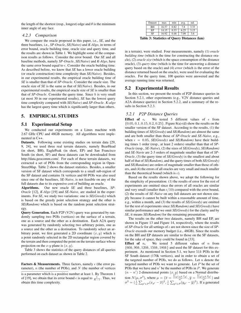
Table 3 shows the statistics of the query distances of all queriesperformed on each dataset as shown in Table 2.

Factors & Measurements. Three factors, namely ε (the error pa-rameter), n (the number of POIs), and N (the number of vertices

is a parameter which is a positive number at least 1. By Theorem 1of [19], we obtain that its error bound ε is equal to 1

K−1. Thus, we

obtain this time complexity.

Dataset max min avg. std.

BH 16.57 0.82 7.8 3.33EP 14.15 0.33 6.25 3.15SF 16.92 0.48 7.09 3.6

Table 3: Statistics of Query Distances (km)

in a terrain), were studied. Four measurements, namely (1) oraclebuilding time (which is the time for constructing the distance ora-cle), (2) oracle size (which is the space consumption of the distanceoracle), (3) query time (which is the time for answering a distancequery based on the oracle) and (4) error (which is the error of thedistance returned based on the oracle), were used for evaluating theoracles. For the query time, 100 queries were answered and theaverage running time was returned.

5.2 Experimental ResultsIn this section, we present the results of P2P distance queries in

Section 5.2.1, other experiments (e.g., V2V distance queries andA2A distance queries) in Section 5.2.2, and a summary of the re-sults in Section 5.2.3.

5.2.1 P2P Distance QueriesEffect of ε. We tested 5 different values of ε from{0.05, 0.1, 0.15, 0.2, 0.25}. Figure 8(a)-(d) show the results on thesmaller version of the SF dataset. According to the results, (1) thebuilding times of SE(Greedy) and SE(Random) are almost the sameand are both smaller than those of SP-Oracle and SE-Naive, e.g.,when ε = 0.05, SE(Greedy) and SE(Random) have their build-ing times 1 order (resp., at least 2 orders) smaller than that of SP-Oracle (resp., SE-Naive), (2) the sizes of SE(Greedy), SE(Random)and SE-Navie are 2-3 orders of magnitude smaller than that of SP-Oracle, (3) the query time of SE(Greedy) is the smallest and abouthalf of that of SE(Random), and the query times of both SE(Greedy)and SE(Random) are orders of magnitude smaller than those of oth-ers, and (4) the errors of all oracles are very small and much smallerthan the theoretical bound (which is ε).

Based on the results shown above, we adopt the following forthe simplicity of presentation: (1) the results of error for the rest ofexperiments are omitted since the errors of all oracles are similarand very small (smaller than ε/10) compared with the error bound,(2) the results of SE-Naive on any full datasets are not shown sim-ply because it cannot be built within a reasonable amount of time,e.g., within a month, and (3) the results of SE(Greedy) are omittedfor the rest of experiments since SE(Random) and SE(Greedy) havesimilar performance and we omit SE(Greedy) for the clarity and bySE, it means SE(Random) for the remaining presentation.

The results on the other two datasets, namely BH nad EP, areshown in Figure 13 and Figure 14, respectively, where the resultsof SP-Oracle for all settings of ε are not shown since the size of SP-Oracle exceeds our memory budget (i.e., 48GB). Since the resultson the BH and EP datasets are similar to those on the SF datasets,for the sake of space, they could be found in [33].Effect of n. We tested 5 different values of n from{60k, 90k, 120k, 150k, 180k} and used the SF dataset for this ex-periment. As mentioned in Section 5.1, we have 51k POIs in theSF South dataset (170k vertices), and in order to obtain a set ofthe targeted number of POIs, we do as follows. Let n denote thetargeted number of POIs we want to generate. Let P be the set ofPOIs that we have and n′ be the number of POIs in P . We generate(n − n′) 2-dimensional points (x, y) based on a Normal distribu-

tion N(µ, σ2), where µ = (x =∑p′∈P xp′n′ , y =

∑p′∈P yp′n′ ) and

σ2 = ( 1n

∑p′∈P (xp′ − x)2, 1

n

∑p′∈P (yp′ − y)2). If a generated

SE SP-Oracle K-Algo

105

106

107

60 90 120 150 180

(a)

Build

ing

Tim

e (s

)

n (k)

100

101

102

103

104

105

106

60 90 120 150 180

(c)

Que

ry T

ime

(ms)

n (k)

102

103

104

105

60 90 120 150 180

(b)

Size

(MB)

n (k)

Figure 9: Effect of n on SF dataset (P2P Distance Queries)

SE K-Algo

105

106

107

0.5 1 1.5 2 2.5

(a)

Build

ing

Tim

e (s

)

N (M)

103

104

105

106

107

0.5 1 1.5 2 2.5

(c)

Que

ry T

ime

(ms)

N (M)

100

101

102

103

0.5 1 1.5 2 2.5

(b)

Size

(MB)

N (M)

Figure 10: Effect of N on BH dataset (P2P Distance Queries)

SE SP-Oracle K-Algo

105

106

107

60 90 120 150 180

(a)

Bui

ldin

g Ti

me

(s)

n (k)

101

102

103

104

105

106

60 90 120 150 180

(c)

Que

ry T

ime

(ms)

n (k)

102

103

104

105

60 90 120 150 180

(b)

Siz

e (M

B)

n (k)

Figure 11: Effect of n on SF dataset (V2V Distance Queries)

point (x, y) is outside the range of the terrain, we simply discardit and re-do the process until a point within the range is generated.At the end, we project each generated point (x, y) to the surface ofthe terrain and take the projected point as a newly generated POI.The results are shown in Figure 9. According the these results, ouroracle SE outperforms SP-Oracle in terms of oracle building time,oracle size and query time and significantly outperforms K-Algo interms of query time.Effect of N . We tested 5 values of N from{0.5M, 1M, 1.5M, 2M, 2.5M} on synthetic datasets. Eachsynthetic dataset with N vertices is a terrain surface from anenlarged BH dataset (4.2M vertices) simplified by a surfacesimplification algorithm [24]. Note that each simplified terrainsurface covers the same region as the original BH dataset with adifferent simplification ratio and still has 4k POIs. The enlargedBH dataset was generated from the BH dataset as follows. On eachface of BH, we added a new vertex on its geometric center and adda new edge between the new vertex and each of the three verticeson the face. The results are shown in Figure 10, where the resultsof SP-Oracle are not shown since the size of SP-Oracle exceedsour memory budget (i.e., 48GB).

5.2.2 Other ExperimentsV2V Distance Queries: In V2V queries, the original POIs are dis-carded, and we treat all vertices as POIs. We varied n and ε forthe experiments. Consider the experiment studying the effect of n.Note that N = n in this experiment. We tested 5 values of n (i.e.,N ) from {60k, 90k, 120k, 150k, 180k} on synthetic datasets, andeach synthetic dataset with N vertices corresponds to a sub-regionof a SF dataset with a higher resolution (10m×10m resolution, 1Mvertices). The results are shown in Figure 11, and according to theresults, SE has its building time and size both at least 1 order ofmagnitude smaller than SP-Oracle and its query time 2-3 (resp.,5-6) orders of magnitude smaller than that of SP-Oracle (resp., K-Algo).

We also conducted the experiment studying the effect of ε withvalues in {0.05, 0.1, 0.15, 0.2, 0.25} on the smaller version of theSF dataset. The results are also similar. In particular, the querytime of SE is 5-6 orders (resp., 6-8 orders) of magnitude smallerthan that of SP-Oracle (resp., K-Algo).Arbitrary Point to Arbitrary Point (A2A) Queries. We testedthe A2A distance queries where the query point is not a POI but anarbitrary point on the terrain surface. We used the low resolution

SE SP-Oracle K-Algo

105

106

107

0.05 0.1 0.15 0.2 0.25

(a)

Build

ing T

ime (

s)

ε

103

104

105

0.05 0.1 0.15 0.2 0.25

(b)

Siz

e (

MB

)

ε

100

101

102

103

104

105

106

107

0.05 0.1 0.15 0.2 0.25

(c)

P2P

Query

Tim

e (

ms)

ε

100

101

102

103

104

105

106

107

0.05 0.1 0.15 0.2 0.25

(d)

A2A

Query

Tim

e (

ms)

ε

Figure 12: P2P Queries In The Case n > N and A2A Queries

BH (resolution: 30 meter, 150k vertices) dataset by varying ε from{0.05, 0.1, 0.15, 0.2, 0.25}. Figure 12(a), (b), and (c) shows thebuilding time, oracle size and query time, respectively. Accordingto the results, SE outperforms SP-Oracle by several times in termsof building time and size. The query time of SE is 2-3 (resp., 5-6)orders of magnitude smaller than that of SP-Oracle (resp., K-Algo).P2P Queries In The Case n > N . We tested P2P queries of thecase n > N on the low resolution BH (resolution: 30 meter, 150kvertices) dataset by varying ε from {0.05, 0.1, 0.15, 0.2, 0.25}. Wegenerated 1M POIs by the same method as mentioned in Sec-tion 5.2.1. Figure 12(a)(b)(d) shows the building time, oracle sizeand query time, respectively. The result is similar to that of A2Aquery. Note that the building time and space of P2P Queries in thecase n > N is the same as those of A2A queries since each testedoracle is the same in the two queries.

5.2.3 Experimental Result SummaryOur SE consistently outperforms the state-of-the-art oracle, i.e.,

SP-Oracle, in terms of all measurements (i.e., building time, oraclesize, and query time) and for any types of distance queries (i.e., P2Pqueries, V2V queries and A2A queries).

6. CONCLUSIONIn this paper, we studied an important spatial query, the shortest

distance query, which is fundamental to many other spatial queriesand many data mining applications. We proposed a distance or-acle called SE which have three good features: (1) low construc-tion time, (2) small size and (3) low query time (compared withthe best-known oracle [12]). Our experimental studies show thatSE consistently outperforms than the best-known algorithm, SP-Oracle, in terms of all measurements for P2P queries, V2V queriesand also A2A queries. There are several interesting research direc-tions. One of them is to study how to efficiently update the distanceoracle when there is an update on some POIs.Acknowledgements: We are grateful to the anonymous review-ers for their constructive comments on this paper. The researchof Victor Junqiu Wei and Raymond Chi-Wing Wong is supportedby HKRGC GRF 16219816. The research of David M. Mount issupported by NSF CCF-1618866.

7. REFERENCES[1] A. Al-Badarneh, H. Najadat, and A. Alraziqi. A classifier to detect

tumor disease in mri brain images. In ASONAM, 2012.[2] L. Aleksandrov, H. N. Djidjev, H. Guo, A. Maheshwari,

D. Nussbaum, and J.-R. Sack. Algorithms for approximate shortestpath queries on weighted polyhedral surfaces. In Discrete &Computational Geometry, 2010.

[3] L. Aleksandrov, A. Maheshwari, and J.-R. Sack. Determiningapproximate shortest paths on weighted polyhedral surfaces. JACM,2005.

[4] A. Beygelzimer, S. Kakade, and J. Langford. Cover trees for nearestneighbor. In ICML, 2006.

[5] P. B. Callahan and S. R. Kosaraju. A decomposition ofmultidimensional point sets with applications to k-nearest-neighborsand n-body potential fields. JACM, 1995.

[6] J. Chen and Y. Han. Shortest paths on a polyhedron. In SOCG, 1990.[7] T. H. Cormen, C. E. Leiserson, R. L. Rivest, and C. Stein.

Introduction to Algorithms. MIT Press and McGraw-Hill, 3rdedition, 2009.

[8] K. Deng, H. T. Shen, K. Xu, and X. Lin. Surface k-nn queryprocessing. In ICDE, 2006.

[9] K. Deng and X. Zhou. Expansion-based algorithms for finding singlepair shortest path on surface. In WWGIS. 2005.

[10] K. Deng, X. Zhou, H. T. Shen, Q. Liu, K. Xu, and X. Lin. Amulti-resolution surface distance model for k-nn query processing.VLDBJ, 2008.

[11] B. G. Dickson and P. Beier. Quantifying the influence of topographicposition on cougar (puma concolor) movement in southern california,usa. Journal of Zoology, 2007.

[12] H. N. Djidjev and C. Sommer. Approximate distance queries forweighted polyhedral surfaces. In ESA. 2011.

[13] M. Fan, H. Qiao, and B. Zhang. Intrinsic dimension estimation ofmanifolds by incising balls. Pattern Recognition, 2009.

[14] J. Fischer and S. Har-Peled. Dynamic well-separated pairdecomposition made easy. In CCCG, 2005.

[15] F. Fodor. The densest packing of 12 congruent circles in a circle.Contributions to Algebra and Geometry, 2000.

[16] J. Golay and M. Kanevski. A new estimator of intrinsic dimensionbased on the multipoint morisita index. Pattern Recognition, 2015.

[17] S. A. Huettel, A. W. Song, and G. McCarthy. Functional magneticresonance imaging. In Sinauer Associates, 2004.

[18] T. Kanai and H. Suzuki. Approximate shortest path on a polyhedralsurface based on selective refinement of the discrete graph and itsapplications. In GMPTA, 2000.

[19] M. Kaul, R. C.-W. Wong, and C. S. Jensen. New lower and upperbounds for shortest distance queries on terrains. VLDB, 2015.

[20] M. Kaul, R. C.-W. Wong, B. Yang, and C. S. Jensen. Finding shortestpaths on terrains by killing two birds with one stone. VLDB, 2013.

[21] B. Kégl. Intrinsic dimension estimation using packing numbers. InNIPS, 2002.

[22] M. Kortgen, G. J. Park, M. Novotni, and R. Klei. 3d shape matchingwith 3d shape contexts. In CESCG, 2003.

[23] J.-F. Lalonde, N. Vandapel, D. F. Huber, and M. Hebert. Naturalterrain classification using three-dimensional ladar data for groundrobot mobility. Journal of field robotics, 2006.

[24] L. Liu and R. C.-W. Wong. Finding shortest path on land surface. InSIGMOD, 2011.

[25] A. Mårell, J. P. Ball, and A. Hofgaard. Foraging and movement pathsof female reindeer: insights from fractal analysis, correlated randomwalks, and lévy flights. Canadian Journal of Zoology, 2002.

[26] J. S. Mitchell, D. M. Mount, and C. H. Papadimitriou. The discretegeodesic problem. SIAM Journal on Computing, 1987.

[27] J. Sankaranarayanan and H. Samet. Distance oracles for spatialnetworks. In ICDE, 2009.

[28] L. T. Sarjakoski, P. Kettunen, H.-M. Flink, M. Laakso,M. Rönneberg, and T. Sarjakoski. Analysis of verbal routedescriptions and landmarks for hiking. Personal and UbiquitousComputing, 2012.

[29] C. Shahabi, L.-A. Tang, and S. Xing. Indexing land surface forefficient knn query. VLDB, 2008.

[30] J. Shotton, J. Winn, C. Rother, and A. Criminisi. Textonboost: Joint

appearance, shape and context modeling for multi-class objectrecognition and segmentation. In ECCV, 2006.

[31] F. Tauheed, L. Biveinis, T. Heinis, F. Schurmann, H. Markram, andA. Ailamaki. Accelerating range queries for brain simulations. InICDE, 2012.

[32] N. Vandapel, R. R. Donamukkala, and M. Hebert. Unmanned groundvehicle navigation using aerial ladar data. The International Journalof Robotics Research, 2006.

[33] V. J. Wei, R. C.-W. Wong, C. Long, and D. M. Mount. Distanceoracle on terrain surface (technical report). Inhttp://www.cse.ust.hk/~raywong/paper/distanceOracle-technical.pdf.

[34] S.-Q. Xin and G.-J. Wang. Improving chen and han’s algorithm onthe discrete geodesic problem. ACM Trans. Graph., 2009.

[35] S. Xing, C. Shahabi, and B. Pan. Continuous monitoring of nearestneighbors on land surface. In VLDB, 2009.

[36] D. Yan, Z. Zhao, and W. Ng. Monochromatic and bichromaticreverse nearest neighbor queries on land surfaces. In CIKM, 2012.

APPENDIXA. LARGEST CAPACITY DIMENSION

Consider a metric spaceX with a distance metric d(·, ·). Given apositive real number r, a set Y ⊆ X is said to be r-separated if forany two distinct points x, y ∈ Y , d(x, y) ≥ r. Given a positive realnumber r and a set S ⊆ X , the r-packing number of S, denotedby M(r, S), is defined to be the maximum cardinality of an r-separated subset of S. Given a metric space X and a distance mea-sure d, a set S ⊆ X and two positive real numbers r1 and r2, thescale-dependent capacity dimension of S w.r.t. r1 and r2, denotedby D(S, r1, r2), is defined to be − logM(r1,S)−logM(r2,S)

log r1−log r2[21].

This dimension is used to measure the ‘intrinsic dimension’ of ametric space. Many high-dimensional data points are believed tobe distributed in a manifold with a low ‘intrinsic dimension’. In-tuitively, the ‘intrinsic dimension’ is the number of independentvariables needed to represent the whole dataset. A good estimateof the ‘intrinsic dimension’ could be used to set the input parame-ters of the dimension reduction algorithms (e.g., Principle Compo-nent Analysis). There are many different specific formulations ofthe ‘intrinsic dimension’ capturing certain properties [21, 13, 16,4]. The scale-dependent capacity dimension captures the geomet-ric property of the data and provides a multi-resolution dimension-ality which depends on the radius r. It measures the growth rate ofM(r, S) w.r.t. r of a subset S of X . In our context, the data spaceX is the set P of all the n POIs and the distance metric d(·, ·) isthe geodesic distance dg(·, ·). Then, we give the definition of a‘ball’ on a terrain surface. Given a point p ∈ P and a non-negativereal number r, a ball centered at p with radius equal to r, denotedby B(p, r), is defined to be a set of all POIs in the disk D(p, r).Then, we give the definition of the capacity dimension of a ballB(p, r) on the terrain surface which only measures the growth rateof M(r,B(p, r)) when r reduces from 2r to r

2.

DEFINITION 1. Given a ball B(p, r) on a terrain surface,where p is a point in P and r is a positive real number, the ca-pacity dimension of B(p, r) is defined to be D(B(p, r), 2r, r

2) =

− logM(2r,B(p,r))−logM( r2,B(p,r))

log 2r−log r2

= 0.5 logM( r

2,B(p,r))

M(2r,B(p,r)).

Consider a set of points whose pairwise geodesic distances areat least 2r. Since the disk D(p, r) could overlap with at most 2 ofthem, we obtain that M(2r,B(p, r)) = 2. Thus, for a given ballB(p, r), the capacity dimension is equal to 0.5 log

M( r2,B(p,r)

2).

Thus, we obtain that given a disk D(p, r), 2 · 22D(B(p,r),2r, r2) is

the maximum number of POIs whose pairwise geodesic distancesare at least r

2such that the disk D(p, r) contains them.

Next, we define the largest capacity dimension of a set P ofPOIs on a terrain surface to be maxp∈P,r∈(0,∞)D(B(p, r), 2r, r

2),

denoted by β. By the definition of the largest capacity dimension,any disk D(p, r), where p is a point in P and r is a positive realnumber, could contain at most 2 · 22β (i.e. O(22β)) POIs whosepairwise geodesic distance is at least r

2.

The definition of largest capacity dimension has an equivalentpresentation as follows. Given a set P of POIs on a terrain surface,its largest capacity dimension β is the largest positive real numbersuch that for any point p in P and any non-negative real number r,the disk D(p, r) overlaps with at most 2 · 22β disjoint disks eachwith radius at least r

4. [15] proved that in the 2D Euclidean space,

a disk with radius r overlaps with at most 12 disjoint disks withradii equal to r

4.029. Thus, in the 2D Euclidean space, a disk with

radius r overlaps with at most 12 disjoint disks with radii equalto r

4. Based on this, we obtain that in an extreme case where the

terrain surface is a 2D plane, the largest capacity dimension β isat most 1.3. In general cases, intuitively, β is a little bit larger than1.3, since the terrain surface could be regarded as a 2D surface withsome fluctuations in terms of height.

B. PROOF

LEMMA 5. Given disks D1(c1, r1) and D2(c2, r2) where (1)c1 and c2 are two points in P and (2) r1 and r2 are two non-negative real numbers, for any point p1 in D1 and any point p2in D2, dg(c1, c2) is an ε-approximate distance of dg(p1, p2) ifdg(c1, c2) ≥ ( 2

ε+ 2) ·max{r1, r2}.

PROOF. By Triangle Inequality, we obtain that dg(c1, c2) −dg(p1, c1)−dg(p2, c2) ≤ dg(p1, p2) ≤ dg(c1, c2) +dg(p1, c1) +dg(p2, c2). Thus, we obtain that dg(p1, p2) − r1 − r2 ≤dg(c1, c2) ≤ dg(p1, p2) + r1 + r2. We further obtain thatdg(p1, p2) ≥ ( 2

ε+ 2) · max{r1, r2} − r1 − r2 ≥ ( 2

ε+

2) · max{r1, r2} − 2 max{r1, r2} = 2ε· max{r1, r2}. By the

two inequalities obtained above, we obtain that dg(p1, p2) − ε ·dg(p1, p2) ≤ dg(c1, c2) ≤ dg(p1, p2) + ε · dg(p1, p2).

PROOF OF LEMMA 1. By Step (b) in the partition tree con-struction algorithm, the tree built satisfies Separation Property andCovering Property. Then, we prove that it also satisfies the dis-tance property: Consider a node O and any of its descendentsO′. Let (O,O1, O2, O3, ......, Ot, O

′) denote the path from Oto O′ in the partition tree. By Separation Property, we obtainthat rOi = rO

2i(1 ≤ i ≤ t), rOt = 2 · rO′ . By our build-

ing method, we obtain that dg(cOi , cOi+1) ≤ rOi(1 ≤ i ≤t − 1), dg(cO, cO1) ≤ rO, dg(cOt , cO′) ≤ rOt . By Trian-gle Inequality, we obtain that dg(cO, cO′) ≤ dg(cO, cO1) +∑t−1i=1 dg(cOi , cOi+1) + dg(cOt , cO′). By integrating all the in-

equalities above, we obtain that dg(cO, cO′) ≤∑ti=0

rO2i≤

2 · rO .

PROOF OF LEMMA 2. Since ∀i ∈ [0, h− 1], ri = 2 · ri+1, weobtain that h = log r0

rh. We obtain that r0 ≤ maxp,q∈P dg(p, q)

since r0 is a geodesic distance between two POIs (the center ofthe root and its farthest neighbor). It is obvious that rh−1 ≥minp,q∈P dg(p, q), since otherwise, ∀p ∈ P , the disk D(p, rh−1)contains only 1 POI and the construction algorithm stops at layerh-1. Since rh =

rh−1

2, we obtain that rh ≥ 0.5·minp,q∈P dg(p, q)

by contradiction.Finally, we obtain that h ≤ log

maxp,q∈P dg(p,q)0.5·minp,q∈P dg(p,q)

.

PROOF OF THEOREM 1. By the algorithm for generating S, weobtain that every pair in S is well-separated at the end. Then, we

prove that for any two points p and q in P , there is exactly one pair〈O,O′〉 containing 〈p, q〉 in S. Consider each iteration of the pro-cedure presented in Section 3.3. We proceed to prove the statement:there is exactly one node pair in S containing 〈p, q〉 at the end ofthe iteration if at the beginning of the iteration, there is exactly onenode pair, denoted by 〈O1, O2〉, in S containing 〈p, q〉. If 〈O1, O2〉is not extracted in the iteration, then 〈O1, O2〉 is still the only onecontaining 〈p, q〉 at the end of the iteration. Otherwise, 〈O1, O2〉 isextracted and w.l.o.g., we assume that O2 is split. Since only onechild of O2 is Oq or an ancestor of Oq , exactly one newly insertednode pair contains 〈p, q〉. Besides, it must be true that at the begin-ning of the first iteration, exactly one node pair (i.e. 〈Oroot , Oroot〉)contains 〈O1, O2〉. By induction, we obtain that at the end of thefinal iteration, exactly one node pair in S contains 〈p, q〉.

Consider the unique pair 〈O,O′〉 containing 〈p, q〉 in thenode pair set of our SE. Since 〈O,O′〉 is well-separated, thendg(O,O

′) ≥ ( 2ε+2)·max{r′O, r′O′}, where r′O (resp., r′O′ ) denote

the radius of the enlarged disk of O (resp., O′). Since the enlargeddisk of O (resp., O′) contains p and q by Distance Property, weobtain that dg(O,O′) = dg(cO, cO′) is an ε-approximate distanceof dg(p, q) by Lemma 5.

LEMMA 6. Consider a chain of node pairs〈O1, O

′1〉, 〈O2, O

′2〉, ..., 〈Oi, O′i〉, ..., 〈Om, O′m〉, where 〈Oi, O′i〉

is generated by 〈Oi−1, O′i−1〉 for each integer i ∈ [2,m]. Let rOi

denote max{rOi , rO′i} for each integer i ∈ [1,m]. ∀k, j ∈ [1,m],rOk ≥ rOj if and only if k < j.

PROOF OF LEMMA 6. It is easy to see that ∀k, j ∈ [1,m]where k < j, Ok (resp., O′k) is Oj (resp., O′j) or an ancestorof Oj (resp., O′j) in Tcompress . Thus, we obtain that rOk ≥ rOjand rO′

k≥ rO′j . Since rOk = max{rOk , rO′k} and rOj =

max{rOj , rO′j}, we obtain that rOk ≥ rOj .

PROOF OF LEMMA 3. Consider the chain of pairs〈O1, O

′1〉, 〈O2, O

′2〉, ..., 〈Oi, O′i〉, ..., 〈Om, O′m〉, where

O1 = O′1 = Oroot , Om = O, O′m = O′ and 〈Oi, O′i〉 isgenerated by 〈Oi−1, O

′i−1〉 for all integer i in [2,m] in our

method of constructing the node pair set of SE. Consider thecase that 〈O,O′〉 is a first-higher-layer node pair. We denotethe parent of O′ in Tcompress by parent(O′), there must existan integer k such that k ∈ [1,m − 1] and parent(O′) is splitfrom 〈Ok, O′k〉. This is because otherwise, 〈O,O′〉 would not begenerated. Consider the pair 〈Ok, O′k〉 from which parent(O′) issplit and thus, rparent(O′) = max{rOk , rO′k}. By Lemma 6, weobtain rparent(O′) ≥ max{rO, rO′} and thus the layer containingparent(O′) is higher than or equal to that containing O. Forthe case that 〈O,O′〉 is a first-lower-layer node pair, the proof issymmetric and we omit the details.

PROOF OF LEMMA 4. Consider a node pair 〈O,O′〉 consid-ered in the procedure described in Section 3.3, where 〈O,O′〉 6=〈Oroot , Oroot〉. Let parent(O) (resp., parent(O′)) denote the par-ent of O (resp., O′) in Tcompress if O (resp., O′) is not the rootnode. It is obvious that 〈O,O′〉 is generated by 〈O, parent(O′)〉or 〈parent(O), O′〉.

W.l.o.g., we assume that 〈O,O′〉 is generated by〈parent(O), O′〉. By Lemma 6, we obtain that rparent(O) ≤rparent(O′) since parent(O′) is split before 〈parent(O), O′〉 isgenerated. By Lemma 3, we obtain that rO′ ≤ rparent(O) andrO ≤ rparent(O′). Let O denote the child of parent(O) in theoriginal partition tree Torg which is on the path from parent(O)to O. There are two cases of O and we present that in both cases,it is true that cO = cO . If O = O, it is obvious that cO = cO .

Then, consider the case where O 6= O. Since any node on the pathfrom O to O excluding O must have only one child, we obtain thatcO = cO by Step (i) of the building algorithm of Torg . Similarly,the child Oc of parent(O′) in the original partition tree Torg

which is on the path from parent(O′) to O′ has the same centerwithO. Since rparent(O) ≤ rparent(O′), we obtain that rO ≤ rOc .Then, consider the node O

′on the path from Oc to O′ in Torg

which is on the same layer as O and has the same center as Oc (ByStep (i), we could always find such a node O). Since cO′ = cO′ ,we obtain that dg(O,O

′) = dg(O,O

′). Since 〈parent(O), O′〉is not a well-separated pair, we obtain that dg(parent(O), O′) ≤2( 2ε

+ 2) · max{rparent(O), rO′} = 2( 2ε

+ 2)rparent(O). Thus,we obtain that dg(parent(O), O

′) ≤ 2( 2

ε+ 2)rparent(O).

Since O is a child of parent(O) in the original par-tition tree Torg , we obtain that dg(parent(O), O) ≤rparent(O) = 2rO . By triangle inequality, we obtain thatdg(O,O

′) ≤ dg(parent(O), O

′) + dg(O, parent(O)) ≤

2( 2ε

+ 2)rparent(O) + 2rO = 4( 2ε

+ 2)rO + 2rO = ( 8ε

+ 10)rO .Thus, 〈O,O′〉 must be an enhanced node pair, where cO = cO andcO′ = cO′ .

LEMMA 7. The maximum number of child nodes of each nodeO in a partition tree or a compressed partition tree is O(22β).

PROOF. By the definition of the partition tree, the center of eachchildren of O must lie in the disk D(cO, rO). Besides, by the Sep-aration Property, the minimum pairwise distance of all its childrenmust be at most rO

2. Thus, by the definition of the largest capacity

dimension β, we obtain that the maximum number of children ofeach node O in a partition tree is O(22β). It is easy to see that theconverting from a partition tree to a compressed partition tree doesnot change the number of children of any undeleted node. Thus,we obtain that the maximum number of children of each node O ina compressed partition tree is O(22β).

LEMMA 8. Any disk D(c, r), where c ∈ P and r is a non-negative real number, can hold at most O((22β)i) points, the min-imum pairwise geodesic distance of which is at least r

2i.

PROOF. Consider a set PSET of points in D(c, r) such thattheir minimum pairwise geodesic distance is at least r

2i. We first

build a partition tree upon PSET as follows: first, we create theroot to be O(cO = c, rO = r) instead of following Step(a) and thebuilding procedure of other nodes is the same as Step(b). Since theradius of each non-root node is half of its parent’s radius, we obtainthat there are totally i layers in the tree. By Lemma 7, we obtainthat the number of children of any node in the compressed partitiontree is at most O(22β). Thus, the number of nodes in Layer i is atmost O(22β) times that in Layer i − 1, where 0 < i ≤ h. Thus,we obtain that there are at most O((22β)i) nodes in the Layer i. Inother words, PSET has at most O((22β)i) points.

LEMMA 9. The compressed partition tree Tcompress has O(n)nodes.

PROOF. Let m, k denote the number of nodes and edges inTcompress , respectively. By the construction of Tcompress , Tcompress

has n leaf nodes and every inner node in Tcompress has at least2 children. Thus, Tcompress has m − n inner nodes and at least2 · (m − n) edges. Since Tcompress is a tree, we obtain thatk = m − 1. Thus, we obtain that k = m − 1 ≥ 2(m − n).Finally, we obtain that m ≤ 2n− 1.

PROOF OF THEOREM 2. Proof Sketch. To give the intuitionof the proof, we present an intermediate node pair set S′ which is

conceptual. Let T ′ denote the tree which is the same as the orig-inal partition tree except that the radius of each leaf node is 0. S′

denote a node pair set built by the node pair generating algorithmpresented in Section 3.3 which takes T ′ as input instead of the com-pressed partition tree. It is clear from a high-level intuition that thenode pair set S of SE is not larger than S′ and the number of thenode pairs considered in the process of generating S is O(|S|) (seethe full proof for the details). In the following, we denote rOx asthe radius of a node Ox in the original partition tree. Consider anode O in T ′ and a set S ′(O) which is {O′|〈O,O′〉 or 〈O′, O〉is in S′ and rO ≥ rO′}. Note that ∪O∈TS ′(O) = S′. By thenode pair generating algorithm, we obtain that for each node O′

in S ′(O), 1. O′ is in the same layer as O or one layer lower thanO (see Lemma 10) 2. there is a upper bound on dg(O,O′), i.e.,O′ lies in a disk D centered at cO′ with a rO- and ε-related ra-dius (see Lemma 11). Then, together with a property (see Lemma8) derived from β, we obtain that |S ′(O)| = O(( 1

ε)2β) and thus

|S′| = O(( 1ε)2βnh).

Detailed Proof. Now, we delve into the detailed proof and adoptthe same notations as shown in the proof sketch.

LEMMA 10. ∀O′ ∈ S ′(O), rO′ ≤ rO ≤ 2 · rO′

PROOF. Since parent(O′) is split before the node pair 〈O,O′〉is generated, by Lemma 6, we obtain rparent(O′) ≥ rO .

Since rparent(O′) = 2 · rO′ , we obtain that rO′ ≤ rO ≤ 2 ·rO′ .

LEMMA 11. ∀O′ ∈ S ′(O), dg(cO, cO′) ≤ (4 2ε

+ 10) · rO .

PROOF. By our node pair set generating algorithm presentedin Section 3.3, 〈O,O′〉 is generated by 〈parent(O), O′〉 or〈O, parent(O′)〉 and the node pair which generated 〈O,O′〉 is notwell separated. Consider the case where 〈O,O′〉 is generated by〈O, parent(O′)〉 (the analysis of the case where 〈O,O′〉 is gen-erated by 〈parent(O), O′〉 is symmetric, i.e., just with O and O′

swapped, and has the same result and thus, we do not present thiscase for the sake of space). We obtain that dg(cO, cparent(O′)) ≤2 · ( 2

ε+ 2) · max{rO, rparent(O′)}, where rparent(O′) = 2rO′

by the definition of the partition tree. By Lemma 10, we obtainthat dg(cO, cparent(O′)) ≤ 2 · ( 2

ε+ 2) · rparent(O′). By Triangle

Inequality, we obtain that dg(cO, cO′) ≤ dg(cO, cparent(O′)) +dg(cO′ , cparent(O′)). By the definition of the partition tree, weobtain that dg(cO′ , cparent(O′)) ≤ rparent(O′). Thus, we obtainthat dg(cO, cO′) ≤ 2 · ( 2

ε+ 2) · rparent(O′) + rparent(O′). By

Lemma 10, we obtain that dg(cO, cO′) ≤ (4 2ε

+ 10) · rO .

Let S ′′ be a point set containing the centers of all nodes inS ′(O). By Lemma 10, we obtain thatO′ is either in the same layeras O in the partition tree or one layer lower than O in the partitiontree. Let S ′′1 (resp., S ′′2 ) denote {O′′|O′′ ∈ S ′′, O′′ is in the samelayer asO} (resp., {O′′|O′′ ∈ S ′′, O′′ is one layer lower thanO}).

By the Separation Property, we obtain that the minimum pair-wise geodesic distance of S ′′1 (resp., S ′′2 ) must be at least rO (resp.,rO2

). By Lemma 8, we obtain that the Disk D(rO, (42ε

+ 10) ·rO) can hold O((22β)log(4

2ε+10)) (resp., O((22β)log(2(4

2ε+10))))

points whose minimum pairwise geodesic distance is at leastrO (resp., rO

2). Thus, we obtain that |S ′(O)| ≤ 2 ·

(22β)log(2·(42ε+10)) = O(( 1

ε)2β). There are at most nh such node

O in T . Thus, we obtain that |S′| is O( nhε2β

) since ∪O∈TS ′(O) =

S′.Next, we prove that |S| is at most |S′| (i.e. O( nh

ε2β)), where S

is the node pair set of SE. Consider a node pair 〈O,O′〉 in S. We

SE K-Algo

105

106

107

0.05 0.1 0.15 0.2 0.25

(a)

Bui

ldin

g Ti

me

(s)

ε

101

102

103

104

0.05 0.1 0.15 0.2 0.25

(b)

Siz

e (M

B)

ε

100

101

102

103

104

105

106

107

0.05 0.1 0.15 0.2 0.25

(c)

Que

ry T

ime

(ms)

ε

Figure 13: Effect of ε on BearHead dataset (P2P Distance Queries)

SE K-Algo

105

106

107

0.05 0.1 0.15 0.2 0.25

(a)

Bui

ldin

g Ti

me

(s)

ε

101

102

103

104

105

0.05 0.1 0.15 0.2 0.25

(b)

Siz

e (M

B)

ε

10-1

100

101

102

103

104

105

106

107

0.05 0.1 0.15 0.2 0.25

(c)

Que

ry T

ime

(ms)

ε

Figure 14: Effect of ε on EaglePeak dataset (P2P Distance Queries)

denote the node in T ′ which comes from the same node in the par-tition tree Torg as O (resp., O′) by Ox (resp., Oy). Since 〈O,O′〉are well-separated, 〈Ox, Oy〉 are well-separated and thus, we couldfind a node pair 〈Ox, Oy〉 in S′ containing 〈Ox, Oy〉. We call〈Ox, Oy〉 the corresponding pair of 〈O,O′〉. Let Op (resp., O′p)denote the node in T ′ which comes from the same node in Torg asthe parent of O (resp., O′) in Tcompress . Op and O′p are not wellseparated, since otherwise, 〈O,O′〉 could not be generated. Ox(resp., Oy) must be on the path from Op (resp., O′p) to Ox (resp.,Oy) and any node on the path excluding Ox and Op (resp., Oy andO′p) must have only one child. Thus, we obtain that any two differ-ent node pairs in S must have different corresponding pairs. Thus,we obtain that |S| ≤ |S′| = O( nh

ε2β). Since in each iteration of

the procedure of generating S, we extract one pair and insert morethan one pair to S. The number of node pairs considered must beat most 2 times the size of the final S and thus it is O( nh

ε2β).

LEMMA 12. The oracle building time of SE is O(N log2 N

ε2β+

nh logn+ nhε2β

).

PROOF. The oracle building time of SE consists of the timetorg of building the original partition tree Torg , the time ttran oftransforming the partition tree to the compressed partition treeTcompressed , the time ten of creating all the enhanced edges andthe time tnp of generating the node pair set of SE. torg consists ofthe running time of B+-tree operations, the point selection algo-rithm and all SSAD algorithms invoked. Note that we index a setof points/nodes with a B+-tree and we find the parent of O in Step(iii) with a SSAD algorithm and dg(O,Oparent) is at most 2rO dueto the covering property. The running time of all the B+-tree opera-tions in torg is O(nh logn) since there are h layers and each layerneeds O(n) insertion/search operation in B+-tree. For the pointselection algorithm, the random selection algorithm takes O(nh)time since there are at most nh nodes in Torg and each takes atmostO(1) time. The greedy selection algorithm takesO(nh logn)time since in each layer since it takes O(n logn) time to create thegrid and corresponding B+-tree in each cell and there are at mostO(n) heap operations and B+-tree operations. It is obvious that theoverall running time of all SSAD algorithms performed in torg issmaller than ten . ttran is O(nh) time since the partition tree hasO(nh) nodes. By Theorem 2, there are at most O( nh

ε2β) node pairs

considered in the procedure described in Section 3.3 and thus, tnpis O( nh

ε2β). Next, we will analyze ten .

We introduce a new parameter of the terrain surface, denoted byθ. θ is defined to be the largest positive real number such that thenumber of vertices on the terrain surface in a diskD(c, r) is at least2θ times the number of vertices on the terrain surface contained inthe disk D(c, r

2), where c is a POI on the terrain surface and r is a

positive real number at most maxp∈V dg(c, p). Thus, the numberof vertices contained in a disk centered at any POI is at most 1

2θ

times that in a disk with double radius and the same center. For theroot nodeOroot , we expand the diskD(cOroot , r0). For any nodeOin other layers, we expand the diskD(cO, l·rO), where l = 8

ε+10.

Note that ∀i ∈ [dlog le, h], l · ri ≤ r0. Since D(c, r0) is a sub-region on the terrain surface, where c is any point on the surface,we obtain that the vertices of terrain visited by SSAD algorithm

invoked for each node in layer i is at mostN, if i ∈ [0, dlog le−1];otherwise, it is N

2θ(i−dlog le).

By Lemma 7, there are at most (22β)i nodes in Layer i. Thus,we obtain that ten is at most O(

∑dlog le−1i=0 (22β)iN log2N +∑h

i=dlog le(22β)iN log2 N

22θ(i−dlog le)) = O(N log2N (22β)dlog le−1

22β−1+

(22β)dlog le∑h−dlog lei=0

(22β)iN log2 N

22θi) =

O((22β)dlog leN log2N∑hi=0( 22β

22θ)i). Our empirical study

verified that θ ≥ β. Thus, we obtain that 22β

22θ< 1 and thus ten is

O((22β)dlog le−1N log2N) = O(N log2 N

ε2β). Thus, we obtain that

the oracle building time is O(N log2 N

ε2β+ nh logn+ nh

ε2β).

PROOF OF THEOREM 3. By Lemma 12, Theorem 2, and theanalysis in Section 3.4, we obtain the result.

C. A2A DISTANCE QUERY PROCESSINGWe present an oracle to answer the arbitrary point-to-arbitrary

point (A2A) distance query based on our proposed distance ora-cle SE. This oracle is the same as that presented in Section 3 ex-cept that it takes some Steiner points introduced as input instead ofall POIs, where Steiner points are introduced by the method pro-posed in [12] (there are O( N

sin(θ)·√ε

log 1ε) Steiner points, where

θ is the minimum inner angle of any face). Then, we present thequery processing. Given two arbitrary points s and t, we first findthe neighborhood of s (resp., t), denoted by N (s) (resp., N (t))(It is a set of Steiner points on the same face containing s (resp.,t) and its adjacent face(s) [12]. Finally, we return d̃g(s, t) =

minp∈N (s),q∈N (t)[dg(s, p) + d̃g(p, q) + dg(q, t)], where dg(s, p)and dg(q, t) could be computed in constant time by SSAD al-gorithm and d̃g(p, q) is the distance between p and q estimatedby the oracle constructed. By [12], |N (s)| · |N (t)| = 1

sin(θ)·ε

and if d̃g(p, q) is an ε-approximate distance of dg(p, q), thend̃g(s, t) is also an ε-approximate distance of dg(s, t). By Theo-rem 3, we obtain that for any two Steiner points p and q, d̃g(p, q)is an ε-approximate distance of dg(p, q) and it takes O(h) timeto compute d̃g(p, q) and the building time (resp., oracle size) is

O(N log2 N

ε2β+ Nh

sin(θ)√ε· log 1

ε· log

N log 1ε

sin(θ)√ε

+ Nhsin(θ)

√ε·ε2β · log 1

ε)

(resp., O( Nhsin(θ)

√ε·ε2β · log 1

ε)). Thus, we obtain that for any two

arbitrary points s and t, the oracle gives an ε-approximate distanceof dg(s, t) and the query time is O( h

sin(θ)·ε ).

D. DISCUSSION FOR CASE WHEN n > N

When n > N , we adopt the same distance oracle describedin Appendix C, which is POI-independent. This distance oraclecould answer not only A2A distance queries but also V2V distancequeries and P2P distance queries (because A2A distance queriescould be regarded as a general setting compared with V2V distancequeries and P2P distance queries).