distance-constrained vehicle routing...
TRANSCRIPT

DISTANCE-CONSTRAINED VEHICLE
ROUTING PROBLEM:
EXACT AND APPROXIMATE SOLUTION
(MATHEMATICAL PROGRAMMING)
A thesis submitted for the degree of Doctor of Philosophy
by
Samira Almoustafa
School of Information Systems, Computing and Mathematics
Brunel University
July 21, 2013
Abstract
The asymmetric distance–constrained vehicle routing problem (ADVRP) looks at finding ve-
hicle tours to connect all customers with a depot, such that the total distance is minimised;
each customer is visited once by one vehicle; every tour starts and ends at a depot; and the
travelled distance by each vehicle is less than or equal to the given maximum value.
We present three basic results in this thesis. In the first one, we present a general flow-
based formulation to ADVRP. It is suitable for symmetric and asymmetric instances. It has
been compared with the adapted Bus School Routing formulation and appears to solve the
ADVRP faster. Comparisons are performed on random test instances with up to 200 customers.
We reach a conclusion that our general formulation outperforms the adapted one. Moreover,
it finds the optimal solution for small test instances quickly. For large instances, there is a
high probability that an optimal solution can be found or at least improve upon the value
of the best feasible solution found so far, compared to the other formulation which stops
because of the time condition. This formulation is more general than Kara formulation since
it does not require the distance matrix to satisfy the triangle inequality.
The second result improves and modifies an old branch-and-bound method suggested by
Laporte et al. in 1987. It is based on reformulating a distance–constrained vehicle routing
problem into a travelling salesman problem and uses the assignment problem as a lower
bounding procedure. In addition, its algorithm uses the best-first strategy and new branching
rules. Since this method was fast but memory consuming, it would stop before optimality
is proven. Therefore, we introduce randomness in choosing the node of the search tree in
case we have more than one choice (usually we choose the smallest objective function). If an
optimal solution is not found, then restart is required due to memory issues, so we restart
our procedure. In that way, we get a multistart branch and bound method. Computational
experiments show that we are able to exactly solve large test instances with up to 1000
customers. As far as we know, those instances are much larger than instances considered
for other VRP models and exact solution approaches from recent literature. So, despite its
simplicity, this proposed algorithm is capable of solving the largest instances ever solved in
i
literature. Moreover, this approach is general and may be used in solving other types of
vehicle routing problems.
In the third result, we use VNS as a heuristic to find the best feasible solution for groups
of instances. We wanted to determine how far the difference is between the best feasible
solution obtained by VNS and the value of optimal solution in order to use the output
of VNS as an initial feasible solution (upper bound procedure) to improve our multistart
method. Unfortunately, based on the search strategy (best first search), using a heuristic to
find an initial feasible solution is not useful. The reason for this is because the branch and
bound is able to find the first feasible solution quickly. In other words, in our method using
a good initial feasible solution as an upper bound will not increase the speed of the search.
However, this would be different for the depth first search. However, we found a big gap
between VNS feasible solution and an optimal solution, so VNS can not be used alone unless
for large test instances when other exact methods are not able to find any feasible solution
because of memory or stopping conditions.
ii
Contents
Abstract i
List of Figures vii
List of Tables x
List of Algorithms xi
List of Abbreviations xii
Acknowledgments xiv
Related Publications xv
1 Introduction 1
1.1 Classification of Vehicle Routing Problems . . . . . . . . . . . . . . . . . . . . 3
1.1.1 Unconstrained Vehicle Routing Problems . . . . . . . . . . . . . . . . 4
1.1.2 Constrained Vehicle Routing Problems . . . . . . . . . . . . . . . . . 5
1.2 VRP Formulation Types . . . . . . . . . . . . . . . . . . . . . . . . . . . . . . 13
1.2.1 Vehicle Flow Formulation . . . . . . . . . . . . . . . . . . . . . . . . . 14
1.2.2 Commodity Flow Formulation . . . . . . . . . . . . . . . . . . . . . . 15
1.2.3 Set-Partitioning Formulation . . . . . . . . . . . . . . . . . . . . . . . 17
1.3 Distance-Constrained Vehicle Routing Problem . . . . . . . . . . . . . . . . . 18
1.3.1 History . . . . . . . . . . . . . . . . . . . . . . . . . . . . . . . . . . . 18
iii
1.3.2 Our Approach . . . . . . . . . . . . . . . . . . . . . . . . . . . . . . . 21
1.4 Thesis Overview . . . . . . . . . . . . . . . . . . . . . . . . . . . . . . . . . . 23
2 Solution Methods 25
2.1 Exact Algorithms . . . . . . . . . . . . . . . . . . . . . . . . . . . . . . . . . . 25
2.1.1 Branch and Bound (B&B) . . . . . . . . . . . . . . . . . . . . . . . . . 26
2.1.2 Cutting Planes . . . . . . . . . . . . . . . . . . . . . . . . . . . . . . . 30
2.1.3 Branch and Cut (B&C) . . . . . . . . . . . . . . . . . . . . . . . . . . 30
2.1.4 Other Approaches . . . . . . . . . . . . . . . . . . . . . . . . . . . . . 30
2.2 Classical Heuristics . . . . . . . . . . . . . . . . . . . . . . . . . . . . . . . . . 31
2.2.1 Constructive Heuristics . . . . . . . . . . . . . . . . . . . . . . . . . . 33
2.2.2 Two Phase Methods . . . . . . . . . . . . . . . . . . . . . . . . . . . . 33
2.2.3 Improvement Heuristics (Local Search) . . . . . . . . . . . . . . . . . 33
2.3 Metaheuristics . . . . . . . . . . . . . . . . . . . . . . . . . . . . . . . . . . . 33
2.3.1 Local Search Based Metaheuristics . . . . . . . . . . . . . . . . . . . . 36
2.3.2 Population Based Metaheuristics . . . . . . . . . . . . . . . . . . . . . 44
2.3.3 Hybrid Metaheuristics . . . . . . . . . . . . . . . . . . . . . . . . . . . 48
2.4 Variable Neighborhood Search Basic Schemes . . . . . . . . . . . . . . . . . . 49
2.4.1 Variable Neighborhood Descent (VND) . . . . . . . . . . . . . . . . . 50
2.4.2 Reduced Variable Neighborhood Search (RVNS) . . . . . . . . . . . . 52
2.4.3 Basic Variable Neighborhood Search (BVNS) . . . . . . . . . . . . . . 53
2.4.4 General Variable Neighborhood Search GVNS . . . . . . . . . . . . . . 54
2.4.5 Skewed Variable Neighborhood Search (SVNS) . . . . . . . . . . . . . 54
2.4.6 Variable Neighborhood Decomposition Search (VNDS) . . . . . . . . . 56
3 General Formulation for ADVRP 57
3.1 Introduction . . . . . . . . . . . . . . . . . . . . . . . . . . . . . . . . . . . . . 58
3.2 Adapted Formulation . . . . . . . . . . . . . . . . . . . . . . . . . . . . . . . . 59
3.3 Kara Formulation . . . . . . . . . . . . . . . . . . . . . . . . . . . . . . . . . . 60
3.4 General Formulation for ADVRP . . . . . . . . . . . . . . . . . . . . . . . . . 61
iv
3.4.1 Illustrative Example . . . . . . . . . . . . . . . . . . . . . . . . . . . . 62
3.5 Computational Results . . . . . . . . . . . . . . . . . . . . . . . . . . . . . . . 63
3.5.1 Tables of Detailed Results . . . . . . . . . . . . . . . . . . . . . . . . . 66
3.6 Conclusion . . . . . . . . . . . . . . . . . . . . . . . . . . . . . . . . . . . . . 69
4 Multistart Branch and Bound for ADVRP 70
4.1 Introduction . . . . . . . . . . . . . . . . . . . . . . . . . . . . . . . . . . . . . 71
4.2 Mathematical Programming Formulations for ADVRP . . . . . . . . . . . . . 72
4.2.1 Flow Based Formulation . . . . . . . . . . . . . . . . . . . . . . . . . . 73
4.2.2 TSP Formulation . . . . . . . . . . . . . . . . . . . . . . . . . . . . . . 74
4.3 Single Start Branch and Bound for ADVRP (RND-ADVRP) . . . . . . . . . . . 75
4.3.1 Upper Bound . . . . . . . . . . . . . . . . . . . . . . . . . . . . . . . . 76
4.3.2 Lower Bounds . . . . . . . . . . . . . . . . . . . . . . . . . . . . . . . 76
4.3.3 Branching Rules . . . . . . . . . . . . . . . . . . . . . . . . . . . . . . 77
4.3.4 Algorithm . . . . . . . . . . . . . . . . . . . . . . . . . . . . . . . . . 78
4.3.5 Illustrative Example . . . . . . . . . . . . . . . . . . . . . . . . . . . . 83
4.4 Multistart Method for ADVRP (MSBB-ADVRP) . . . . . . . . . . . . . . . . . . . 89
4.4.1 Algorithm . . . . . . . . . . . . . . . . . . . . . . . . . . . . . . . . . . 89
4.4.2 Illustrative Example . . . . . . . . . . . . . . . . . . . . . . . . . . . . 91
4.5 An efficient Implementation - Data Structure . . . . . . . . . . . . . . . . . . 92
4.6 Computational Results . . . . . . . . . . . . . . . . . . . . . . . . . . . . . . 94
4.6.1 Methods Compared. . . . . . . . . . . . . . . . . . . . . . . . . . . . . 96
4.6.2 Numerical Analysis . . . . . . . . . . . . . . . . . . . . . . . . . . . . . 102
4.7 Conclusion . . . . . . . . . . . . . . . . . . . . . . . . . . . . . . . . . . . . . 109
5 Variable Neighborhood Search for ADVRP 111
5.1 Initialization Algorithms . . . . . . . . . . . . . . . . . . . . . . . . . . . . . . 111
5.1.1 INIT-TSP algorithm . . . . . . . . . . . . . . . . . . . . . . . . . . . . 112
5.1.2 INIT-ADVRP Algorithm . . . . . . . . . . . . . . . . . . . . . . . . . . . 112
5.2 VNS-ADVRP Algorithm for ADVRP . . . . . . . . . . . . . . . . . . . . . . . . 114
v
5.2.1 Shaking Agorithms . . . . . . . . . . . . . . . . . . . . . . . . . . . . . 116
5.2.2 Local Search Algorithm . . . . . . . . . . . . . . . . . . . . . . . . . . 117
5.2.3 Illustrative Example . . . . . . . . . . . . . . . . . . . . . . . . . . . . 119
5.3 Computational Results . . . . . . . . . . . . . . . . . . . . . . . . . . . . . . . 127
5.3.1 Data Structure . . . . . . . . . . . . . . . . . . . . . . . . . . . . . . . 128
5.3.2 Numerical Analysis . . . . . . . . . . . . . . . . . . . . . . . . . . . . . 128
5.4 Conclusion . . . . . . . . . . . . . . . . . . . . . . . . . . . . . . . . . . . . . 129
6 Conclusions 131
6.1 Overview . . . . . . . . . . . . . . . . . . . . . . . . . . . . . . . . . . . . . . 131
6.2 Contribution . . . . . . . . . . . . . . . . . . . . . . . . . . . . . . . . . . . . 132
6.3 Future Research . . . . . . . . . . . . . . . . . . . . . . . . . . . . . . . . . . 133
Bibliography 134
Appendix A MSBB Tables of Results 148
.1 Tables of Results for Group 1 . . . . . . . . . . . . . . . . . . . . . . . . . . . 149
.2 Tables of Results for Group 2 . . . . . . . . . . . . . . . . . . . . . . . . . . . 160
.3 Tables of Results for Group 3 . . . . . . . . . . . . . . . . . . . . . . . . . . . 170
Appendix B VNS Tables of Results 179
.4 Tables of Results in Stage 1 . . . . . . . . . . . . . . . . . . . . . . . . . . . . 179
.5 Tables of some Results in Stage 2 . . . . . . . . . . . . . . . . . . . . . . . . . 191
vi
List of Figures
3.1 Optimal solution (n=8, m=2, Dmax =23) . . . . . . . . . . . . . . . . . . . . 63
4.1 Solutions at node 1 (root node), node 2, node 3, and node 4 . . . . . . . . . . 85
4.2 TOL-ADVRP Tree . . . . . . . . . . . . . . . . . . . . . . . . . . . . . . . . . . 87
4.3 Solution at node 5 and 9 . . . . . . . . . . . . . . . . . . . . . . . . . . . . . . 88
4.4 First two iterations . . . . . . . . . . . . . . . . . . . . . . . . . . . . . . . . . 92
4.5 Third iteration . . . . . . . . . . . . . . . . . . . . . . . . . . . . . . . . . . . 94
4.6 % of solved and % of (Feas=Opt) of Group 1 in all stages . . . . . . . . . . . 103
4.7 % of solved and % of (Feas=Opt) of Group 2 in all stages . . . . . . . . . . . 103
4.8 % of solved and % of (Feas=Opt) of Group 3 in all stages . . . . . . . . . . . 104
4.9 Average time for instances in Group 1 . . . . . . . . . . . . . . . . . . . . . . 105
4.10 Average time for instances in Group 2 . . . . . . . . . . . . . . . . . . . . . . 106
4.11 Average time for instances in Group 3 . . . . . . . . . . . . . . . . . . . . . . 107
4.12 Effectiveness and efficiency for instances of all groups in all stages . . . . . . 108
5.1 Current solution before and after insertion (A,B,C) . . . . . . . . . . . . . . . 125
5.2 Solutions after insertion (D,E,F) . . . . . . . . . . . . . . . . . . . . . . . . . 126
vii
List of Tables
3.1 Original distance matrix for ADVRP with n=8 and m=2 . . . . . . . . . . . 62
3.2 Summary results on small test instances . . . . . . . . . . . . . . . . . . . . . 64
3.3 Summary results on large test instances . . . . . . . . . . . . . . . . . . . . . 65
3.4 Table of small instances . . . . . . . . . . . . . . . . . . . . . . . . . . . . . . 66
3.5 Table of small instances (continue) . . . . . . . . . . . . . . . . . . . . . . . . 67
3.6 Table of small instances (continue) . . . . . . . . . . . . . . . . . . . . . . . . 68
3.7 Table of small instances (continue) . . . . . . . . . . . . . . . . . . . . . . . . 69
4.1 Original distance matrix for ADVRP with n=8 and m=2 . . . . . . . . . . . 83
4.2 New distance matrix . . . . . . . . . . . . . . . . . . . . . . . . . . . . . . . . 84
4.3 Results for instances from group 1 with Dmax(1) = ∞ . . . . . . . . . . . . . . 97
4.4 Results for instances from group 1 with Dmax(2) = 0.90× LT (1) . . . . . . . . 98
4.5 Results for instances from group 1 with Dmax(3) = 0.90× LT (2) . . . . . . . . 99
4.6 Results for instances from group 2 with Dmax(1) = ∞ . . . . . . . . . . . . . . 99
4.7 Results for instances from group 2 with Dmax(2) = 0.90× LT (1) . . . . . . . . 100
4.8 Results for instances from group 2 with Dmax(3) = 0.90× LT (2) . . . . . . . . 100
4.9 Results for instances from group 3 with Dmax(1) = ∞ . . . . . . . . . . . . . . 101
4.10 Results for instances from group 3 with Dmax(2) = 0.90× LT (1) . . . . . . . . 101
4.11 Results for instances from group 3 with Dmax(3) = 0.90× LT (2) . . . . . . . . 102
5.1 Distance matrix for ADVRP with n=8 and m=2 . . . . . . . . . . . . . . . 120
5.2 Summary results for instances from group 1, 2, 3 with Dmax(1) = ∞ . . . . . 129
viii
1 Table of results for instances from group 1 with Dmax(1) = ∞ . . . . . . . . . 149
2 Table of results for instances from group 1 with Dmax(1) = ∞ (continue) . . . 150
3 Table of results for instances from group 1 with Dmax(1) = ∞ (continue) . . . 151
4 Table of results for instances from group 1 with Dmax(1) = ∞ (continue) . . . 152
5 Table of results for instances from group 1 with Dmax(2) = 0.90× LT (1) . . . 153
6 Table of results for instances from group 1 with Dmax(2) (continue) . . . . . . 154
7 Table of results for instances from group 1 with Dmax(2) (continue) . . . . . . 155
8 Table of results for instances from group 1 with Dmax(2) (continue) . . . . . . 156
9 Table of results for instances from group 1 with Dmax(3) = 0.90× LT (2) . . . 157
10 Table of results for instances from group 1 with Dmax(3) (continue) . . . . . . 158
11 Table of results for instances from group 1 with Dmax(3) (continue) . . . . . . 159
12 Table of results for instances from group 2 with Dmax(1) = ∞ . . . . . . . . . 160
13 Table of results for instances from group 2 with Dmax(1) = ∞ (continue) . . . 161
14 Table of results for instances from group 2 with Dmax(1) = ∞ (continue) . . . 162
15 Table of results for instances from group 2 with Dmax(1) = ∞ (continue) . . . 163
16 Table of results for instances from group 2 with Dmax(2) = 0.90× LT (1) . . . 164
17 Table of results for instances from group 2 with Dmax(2) (continue) . . . . . . 165
18 Table of results for instances from group 2 with Dmax(2) (continue) . . . . . . 166
19 Table of results for instances from group 2 with Dmax(2) (continue) . . . . . . 167
20 Table of results for instances from group 2 with Dmax(3) = 0.90× LT (2) . . . 168
21 Table of results for instances from group 2 with Dmax(3) (continue) . . . . . . 169
22 Table of results for instances from group 3 with Dmax(1) = ∞ . . . . . . . . . 170
23 Table of results for instances from group 3 with Dmax(1) = ∞ (continue) . . . 171
24 Table of results for instances from group 3 with Dmax(1) = ∞ (continue) . . . 172
25 Table of results for instances from group 3 with Dmax(1) = ∞ (continue) . . . 173
26 Table of results for instances from group 3 with Dmax(2) = 0.90× LT (1) . . . 174
27 Table of results for instances from group 3 with Dmax(2) (continue) . . . . . . 175
28 Table of results for instances from group 3 with Dmax(2) (continue) . . . . . . 176
29 Table of results for instances from group 3 with Dmax(3) = 0.90× LT (2) . . . 177
ix
30 Table of results for instances from group 3 with Dmax(3) (continue) . . . . . 178
31 Table of results for instances from group 1 with Dmax(1) = ∞ . . . . . . . . . 179
32 Table of results for instances from group 1 with Dmax(1) = ∞ (Continue) . . 180
33 Table of results for instances from group 1 with Dmax(1) = ∞ (Continue) . . 181
34 Table of results for instances from group 1 with Dmax(1) = ∞ (Continue) . . 182
35 Table of results for instances from group 2 with Dmax(1) = ∞ . . . . . . . . . 183
36 Table of results for instances from group 2 with Dmax(1) = ∞ (Continue) . . 184
37 Table of results for instances from group 2 with Dmax(1) = ∞ (Continue) . . 185
38 Table of results for instances from group 2 with Dmax(1) = ∞ (Continue) . . 186
39 Table of results for instances from group 3 with Dmax(1) = ∞ . . . . . . . . . 187
40 Table of results for instances from group 3 with Dmax(1) = ∞ (Continue) . . 188
41 Table of results for instances from group 3 with Dmax(1) = ∞ (Continue) . . 189
42 Table of results for instances from group 3 with Dmax(1) = ∞ (Continue) . . 190
43 Table of results for instances from group 1 with Dmax(2) = 0.90× LT (1) . . . 191
44 Table of results for instances from group 1 with Dmax(2) (continue) . . . . . . 192
45 Table of results for instances from group 1 with Dmax(2) (continue) . . . . . . 193
x
List of Algorithms
1 Algorithm of Neighborhood Change . . . . . . . . . . . . . . . . . . . . . . . . 50
2 Algorithm of Best Improvement . . . . . . . . . . . . . . . . . . . . . . . . . . 50
3 Algorithm of First Improvement . . . . . . . . . . . . . . . . . . . . . . . . . . 51
4 Basic VND Algorithm . . . . . . . . . . . . . . . . . . . . . . . . . . . . . . . 52
5 RVNS Algorithm . . . . . . . . . . . . . . . . . . . . . . . . . . . . . . . . . . 53
6 BVNS Algorithm . . . . . . . . . . . . . . . . . . . . . . . . . . . . . . . . . . 53
7 GVNS Algorithm . . . . . . . . . . . . . . . . . . . . . . . . . . . . . . . . . . 54
8 SVNS Algorithm . . . . . . . . . . . . . . . . . . . . . . . . . . . . . . . . . . 55
9 Algorithm of Neighborhood Change for SVNS . . . . . . . . . . . . . . . . . . 55
10 VNDS Algorithm . . . . . . . . . . . . . . . . . . . . . . . . . . . . . . . . . . 56
11 (TOL-ADVRP) Algorithm (β = 0) and (RND-ADVRP) Algorithm (β = 1) . . . . . 81
12 Algorithm of Multistart B&B (MSBB-ADVRP) . . . . . . . . . . . . . . . . . . . 90
13 Algorithm of INIT-TSP for initial solution to TSP . . . . . . . . . . . . . . . . 113
14 Algorithm of INIT-ADVRP . . . . . . . . . . . . . . . . . . . . . . . . . . . . . . 114
15 Algorithm of VNS for ADVRP . . . . . . . . . . . . . . . . . . . . . . . . . . 115
16 Algorithm of Shaking . . . . . . . . . . . . . . . . . . . . . . . . . . . . . . . . 116
17 Algorithm of Shake1 . . . . . . . . . . . . . . . . . . . . . . . . . . . . . . . . 116
18 Algorithm of Shake2 . . . . . . . . . . . . . . . . . . . . . . . . . . . . . . . . 117
19 Algorithm of Local Search . . . . . . . . . . . . . . . . . . . . . . . . . . . . . 118
xi
List of Abbreviations
LP : Linear Program
IP : Integer Linear Program
MIP : Mixed Integer Linear Program
COP : Combinatorial Optimization Problem
VRP : Vehicle Routing Problem
CVRP : Capacitated Vehicle Routing Problem
DVRP : Distance-Constrained Vehicle Routing Problem
ADVRP : Asymmetric Distance-Constrained Vehicle Routing Problem
DCVRP : Distance-Constrained Capacitated Vehicle Routing Problem
VRPTW : Vehicle Routing Problem with Time Windows
VRPB : Vehicle Routing Problem with Backhauls
VRPPD : Vehicle Routing Problem with Pickup and Delivery
NP-hard : Non-Deterministic Polynomial-time hard
TSP : Travelling Salesman Problem
m-TSP : Multiple Travelling Salesman Problem
AP : Assignment Problem
BSRP : Bus School Routing Problem
ABSRP : Adapted Bus School Routing Problem
B&B : Branch and Bound
B&C : Branch and Cut
UB : Upper Bound
LB : Lower Bound
Dmax : Maximum Possible Distance Travelled
N : Number of Customers
V : Set of Vertices
xii
SA : Simulated Annealing
DA : Deterministic Annealing
TS : Tabu Search
GRASP : Greedy Randomized Adaptive Search Procedure
NN : Neural Networks
GLS : Guided Local Search
GAs : Genetic Algorithms
SS : Scatter Search
ACO : Ant Colony Optimization
EA : Evolutionary Algorithm
PR : Path Relinking
VNS : Variable Neighborhood Search
VND : Variable Neighborhood Descent
RVNS : Reduced VNS
BVNS : Basic VNS
GVNS : General VNS
SVNS : Skewed VNS
VNDS : Variable Neighborhood Decomposition Search
MSBB-ADVRP : Multistart B&B Method for ADVRP
RND-ADVRP : Single Start of B&B Method for ADVRP
TOL-ADVRP : Tolerance Based B&B for ADVRP
CPLEX-ADVRP : Commercial software for solving ADVRP
VNS-ADVRP : Variable Neighborhood Search for solving ADVRP
xiii

Acknowledgments
Thank GOD for having a chance to do the research and for being with me in difficult times.
I would like to thank my supervisor Dr Nenad Mladenovic who deserve my sincere thanks
for his great discussion, help and comments during my research. In addition, I want to thank
Professor Dr Said Hanafi for his valuable suggestions and comments. I am grateful to my
colleagues in the department of mathematical sciences in Brunel University for a nice time
and support during my research.
I am warmly thank my husband Talal Dairani for his invaluable support and patient
during the research (Talal, you are great!), and my daughters Nour and Hiba (your smile at
the end of every day encourage me to continue).
The final debts, are:
To my country ”SYRIA” who bore the burden.
To my Father and Mother for unconditional support and encouragement (I did it for
you!).
To my brothers and sisters for believing in me.
To my friends who always support me.
Samira Almoustafa
xiv
Related Publications
• Conference Papers:
– S. Almoustafa, B. Goldengorin, M. Tso, and N. Mladenovic. Two new exact meth-
ods for asymmetric distance-constrained vehicle routing problem. Proceedings of
SYM-OP-IS, pages 297-300, September 2009 [Chapter 4].
– S. Almoustafa, S. Hanafi, and N. Mladenovic. Multistart approach for exact
vehicle routing; Proceedings of Balcor, pages 162-170, 2011 [Chapter 4].
– S. Almoustafa, S. Hanafi, and N. Mladenovic. New formulation for the distance-
constrained vehicle routing problem. Proceedings of SYM-OP-IS, pages 383-387,
2011 [Chapter 3].
• Other Publications:
– S. Almoustafa, S. Hanafi, and N. Mladenovic. Multistart Branch and Bound for
Large Asymmetric Distance-Constrained Vehicle Routing Problem. Les Cahiers
du GERAD. G-2011-29. June 2011.
– S. Almoustafa, S. Hanafi, and N. Mladenovic. Multistart branch and bound for
large asymmetric distance-constrained vehicle routing problem. In: A. Migdalas
and A. Sifaleras and C.K. Georgiadis and J. Papathanasiou and E. Stiakakis, eds.,
Optimization Theory, Decision Making, and Operational Research Applications.
Chapter 2, pages 15–38. Springer, 2012.
– S. Almoustafa, S. Hanafi, and N. Mladenovic. New exact method for large asym-
metric distance-constrained vehicle routing problem. European Journal of Oper-
ational Research, 226(3): 386-394, 2013.
xv
Chapter 1
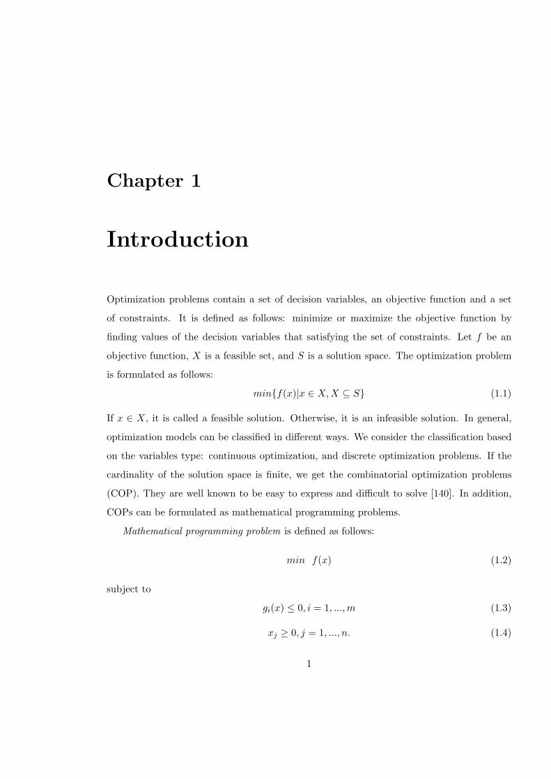
Introduction
Optimization problems contain a set of decision variables, an objective function and a set
of constraints. It is defined as follows: minimize or maximize the objective function by
finding values of the decision variables that satisfying the set of constraints. Let f be an
objective function, X is a feasible set, and S is a solution space. The optimization problem
is formulated as follows:
min{f(x)|x ∈ X, X ⊆ S} (1.1)
If x ∈ X, it is called a feasible solution. Otherwise, it is an infeasible solution. In general,
optimization models can be classified in different ways. We consider the classification based
on the variables type: continuous optimization, and discrete optimization problems. If the
cardinality of the solution space is finite, we get the combinatorial optimization problems
(COP). They are well known to be easy to express and difficult to solve [140]. In addition,
COPs can be formulated as mathematical programming problems.
Mathematical programming problem is defined as follows:
min f(x) (1.2)
subject to
gi(x) ≤ 0, i = 1, ..., m (1.3)
xj ≥ 0, j = 1, ..., n. (1.4)
1
Introduction CHAPTER 1. INTRODUCTION
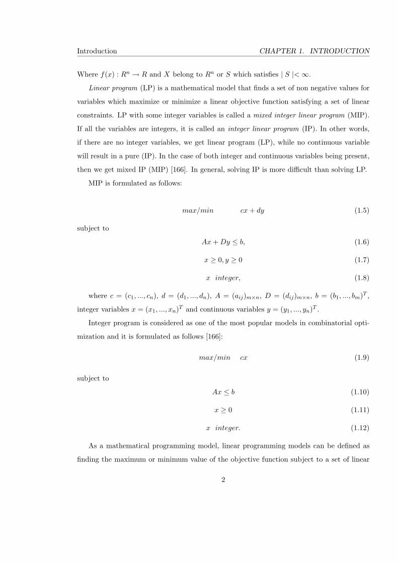
Where f(x) : Rn → R and X belong to Rn or S which satisfies | S |< ∞.
Linear program (LP) is a mathematical model that finds a set of non negative values for
variables which maximize or minimize a linear objective function satisfying a set of linear
constraints. LP with some integer variables is called a mixed integer linear program (MIP).
If all the variables are integers, it is called an integer linear program (IP). In other words,
if there are no integer variables, we get linear program (LP), while no continuous variable
will result in a pure (IP). In the case of both integer and continuous variables being present,
then we get mixed IP (MIP) [166]. In general, solving IP is more difficult than solving LP.
MIP is formulated as follows:
max/min cx + dy (1.5)
subject to
Ax + Dy ≤ b, (1.6)
x ≥ 0, y ≥ 0 (1.7)
x integer, (1.8)
where c = (c1, ..., cn), d = (d1, ..., dn), A = (aij)m×n, D = (dij)m×n, b = (b1, ..., bm)T ,
integer variables x = (x1, ..., xn)T and continuous variables y = (y1, ..., yn)T .
Integer program is considered as one of the most popular models in combinatorial opti-
mization and it is formulated as follows [166]:
max/min cx (1.9)
subject to
Ax ≤ b (1.10)
x ≥ 0 (1.11)
x integer. (1.12)
As a mathematical programming model, linear programming models can be defined as
finding the maximum or minimum value of the objective function subject to a set of linear
2
Introduction Classification of VRP
constraints. In other words, find the values of n decision variables xi to maximize or minimize
the objective function z. It can be written as follows where ci, aij , bi are constants.:
max/min z =n∑
i=1
cixi (1.13)
subject ton∑
j=1
aijxj ≤ bi ∀ i = 1, ..., m (1.14)
xi ≥ 0 ∀ i = 1, ..., n. (1.15)
When the decision variables satisfy the linear constraints, they produce feasible solutions
to the linear programming problem. The feasible region contains all feasible solutions, where
the optimal solution is a feasible solution that optimizes the objective function.
An example of practical combinatorial optimization problem is Vehicle routing problem
(VRP) which is considered as a pure IP problem. In this thesis we are interested in finding
the optimal solution or an approximate solution to one type of VRPs. In the next section
there are definitions, classifications, and formulations for VRPs.
1.1 Classification of Vehicle Routing Problems
Vehicle routing problem (VRP) is defined as planning least cost tours to serve a set of
customers (collection, delivery or both) by using a set of vehicles provided that some con-
straints are satisfied [158]. The objective is to minimize the cost (time or distance) for all
tours. The cost of the tours can be fuel cost, driver wages and so on. It is an NP–hard
problem [75, 141, 168], for information on computational complexity see [96].
Real world applications may be mail delivery, solid waste collection, street cleaning,
distribution of commodities, design telecommunication, transportation networks, school bus
routing, dial–a–ride systems, transportation of handicapped persons, and routing of sales
people and maintenance units. A survey of real–world applications is in [160].
The first article on VRP was published in 1959 by Dantzig and Ramser [40]. Since then,
many researchers have studied various VRP models, mainly driven by the great potential
of its applications as well as its limitations. For a summary about developments of VRP
3
Introduction Classification of VRP
in the last 50 years see [107], which shows the solved instances with up to 135 customers.
Moreover, there are some books for VRPs see [68, 69, 160]. In addition, for an overview of
VRPs we refer to [38, 49, 69, 160, 169].
The VRP can be considered as a generalization of the Multiple Travelling Salesman
Problem (m–TSP), which is also an NP–hard problem. Lenstra and Rinnooy Kan [120]
suggested transforming VRP into m–TSP by adding (m − 1) dummy vertices (where m is
the number of vehicles). The number of vehicles in the VRP corresponds to the number of
salesmen.
There are many different classification principles to VRPs: based on data (static and
dynamic); based on constraints (constrained and unconstrained). In this thesis we classify
VRP problems based on constraints: unconstrained VRP and constrained VRP.
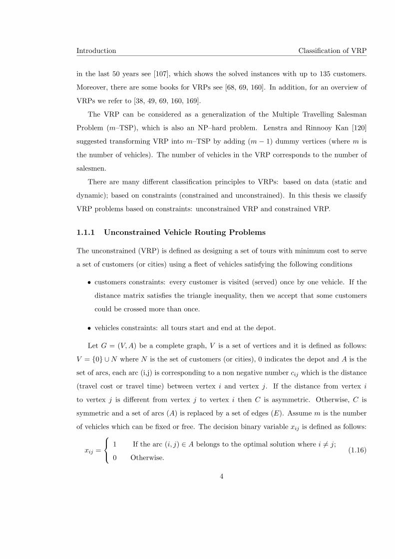
1.1.1 Unconstrained Vehicle Routing Problems
The unconstrained (VRP) is defined as designing a set of tours with minimum cost to serve
a set of customers (or cities) using a fleet of vehicles satisfying the following conditions
• customers constraints: every customer is visited (served) once by one vehicle. If the
distance matrix satisfies the triangle inequality, then we accept that some customers
could be crossed more than once.
• vehicles constraints: all tours start and end at the depot.
Let G = (V, A) be a complete graph, V is a set of vertices and it is defined as follows:
V = {0} ∪N where N is the set of customers (or cities), 0 indicates the depot and A is the
set of arcs, each arc (i,j) is corresponding to a non negative number cij which is the distance
(travel cost or travel time) between vertex i and vertex j. If the distance from vertex i
to vertex j is different from vertex j to vertex i then C is asymmetric. Otherwise, C is
symmetric and a set of arcs (A) is replaced by a set of edges (E). Assume m is the number
of vehicles which can be fixed or free. The decision binary variable xij is defined as follows:
xij =
1 If the arc (i, j) ∈ A belongs to the optimal solution where i 6= j;
0 Otherwise.(1.16)
4
Introduction Classification of VRP
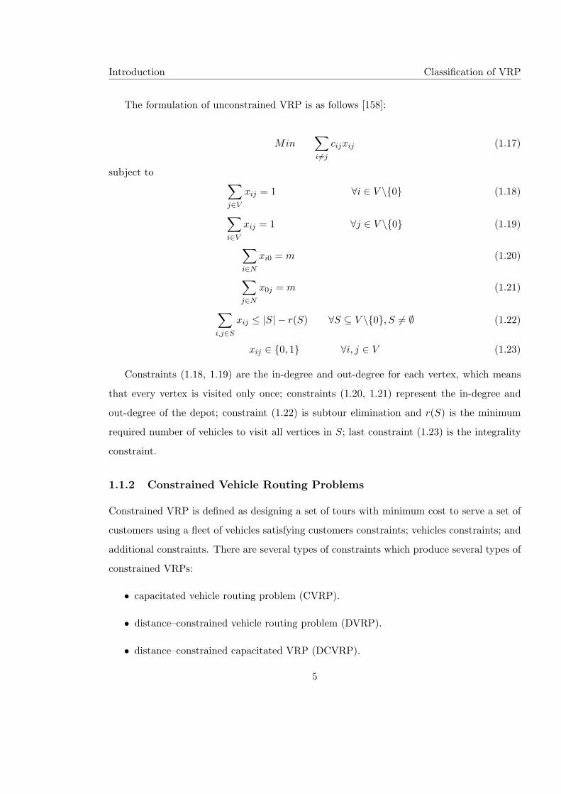
The formulation of unconstrained VRP is as follows [158]:
Min∑
i6=j
cijxij (1.17)
subject to∑
j∈V
xij = 1 ∀i ∈ V \{0} (1.18)
∑
i∈V
xij = 1 ∀j ∈ V \{0} (1.19)
∑
i∈N
xi0 = m (1.20)
∑
j∈N
x0j = m (1.21)
∑
i,j∈S
xij ≤ |S| − r(S) ∀S ⊆ V \{0}, S 6= ∅ (1.22)
xij ∈ {0, 1} ∀i, j ∈ V (1.23)
Constraints (1.18, 1.19) are the in-degree and out-degree for each vertex, which means
that every vertex is visited only once; constraints (1.20, 1.21) represent the in-degree and
out-degree of the depot; constraint (1.22) is subtour elimination and r(S) is the minimum
required number of vehicles to visit all vertices in S; last constraint (1.23) is the integrality
constraint.
1.1.2 Constrained Vehicle Routing Problems
Constrained VRP is defined as designing a set of tours with minimum cost to serve a set of
customers using a fleet of vehicles satisfying customers constraints; vehicles constraints; and
additional constraints. There are several types of constraints which produce several types of
constrained VRPs:
• capacitated vehicle routing problem (CVRP).
• distance–constrained vehicle routing problem (DVRP).
• distance–constrained capacitated VRP (DCVRP).
5
Introduction Classification of VRP
• vehicle routing problem with time windows (VRPTW).
• vehicle routing problem with backhauls (VRPB).
• vehicle routing problem with pickup and delivery (VRPPD).
We will provide the definitions and formulations for each type of VRP, although we will focus
on Asymmetric DVRP in more detail later in this thesis.
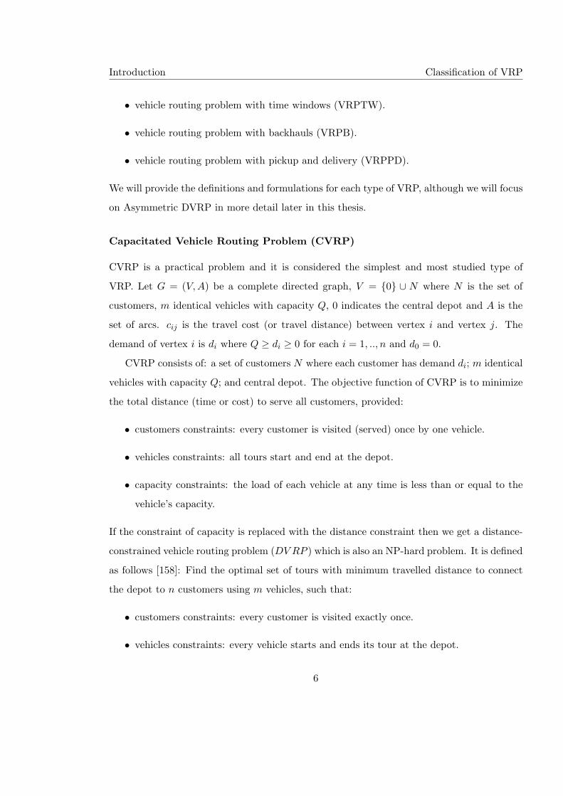
Capacitated Vehicle Routing Problem (CVRP)
CVRP is a practical problem and it is considered the simplest and most studied type of
VRP. Let G = (V, A) be a complete directed graph, V = {0} ∪ N where N is the set of
customers, m identical vehicles with capacity Q, 0 indicates the central depot and A is the
set of arcs. cij is the travel cost (or travel distance) between vertex i and vertex j. The
demand of vertex i is di where Q ≥ di ≥ 0 for each i = 1, .., n and d0 = 0.
CVRP consists of: a set of customers N where each customer has demand di; m identical
vehicles with capacity Q; and central depot. The objective function of CVRP is to minimize
the total distance (time or cost) to serve all customers, provided:
• customers constraints: every customer is visited (served) once by one vehicle.
• vehicles constraints: all tours start and end at the depot.
• capacity constraints: the load of each vehicle at any time is less than or equal to the
vehicle’s capacity.
If the constraint of capacity is replaced with the distance constraint then we get a distance-
constrained vehicle routing problem (DV RP ) which is also an NP-hard problem. It is defined
as follows [158]: Find the optimal set of tours with minimum travelled distance to connect
the depot to n customers using m vehicles, such that:
• customers constraints: every customer is visited exactly once.
• vehicles constraints: every vehicle starts and ends its tour at the depot.
6
Introduction Classification of VRP
• distance constraints: the total travelled distance by each vehicle in the solution is less
than or equal to the maximum possible travelled distance.
It is an asymmetric DVRP if the distance from vertex i to vertex j is different from vertex
j to vertex i. Otherwise, the symmetric DVRP is defined. When the problem of VRP
has distance constraints and capacity constraints, it is called Distance-constrained CVRP
(DCVRP).
If we have only one vehicle with unlimited capacity or no distance constraint, the CVRP
(DVRP, or DCVRP) will be equivalent to the TSP. The solution in this case entails looking
for one tour over all customers with minimum cost or minimum travelled distance [158].
Different types of formulations for CVRP can be found in this thesis in Section (1.2).
Vehicle Routing Problem with Time Windows (VRPTW)
VRPTW is considered as an extension to CVRP with time window constraint and it is also
an NP-hard problem. It is defined as optimizing a set of least cost tours to serve a set of
customers within a time window interval by using a set of vehicles satisfying:
• customers constraints: every customer is visited (served) once by one vehicle. If the
distance matrix satisfies the triangle inequality, then a customer could be crossed more
than once.
• vehicles constraints: all tours start and end at the depot.
• capacity constraints: the load of each vehicle is less than or equal the vehicle’s capacity.
• service time constraints: each customer has to be served within a time window [ai, bi].
That means it is not acceptable to serve customers before or after a time window
interval, and in the case that the vehicle arrives before the start time then it has to
wait [34].
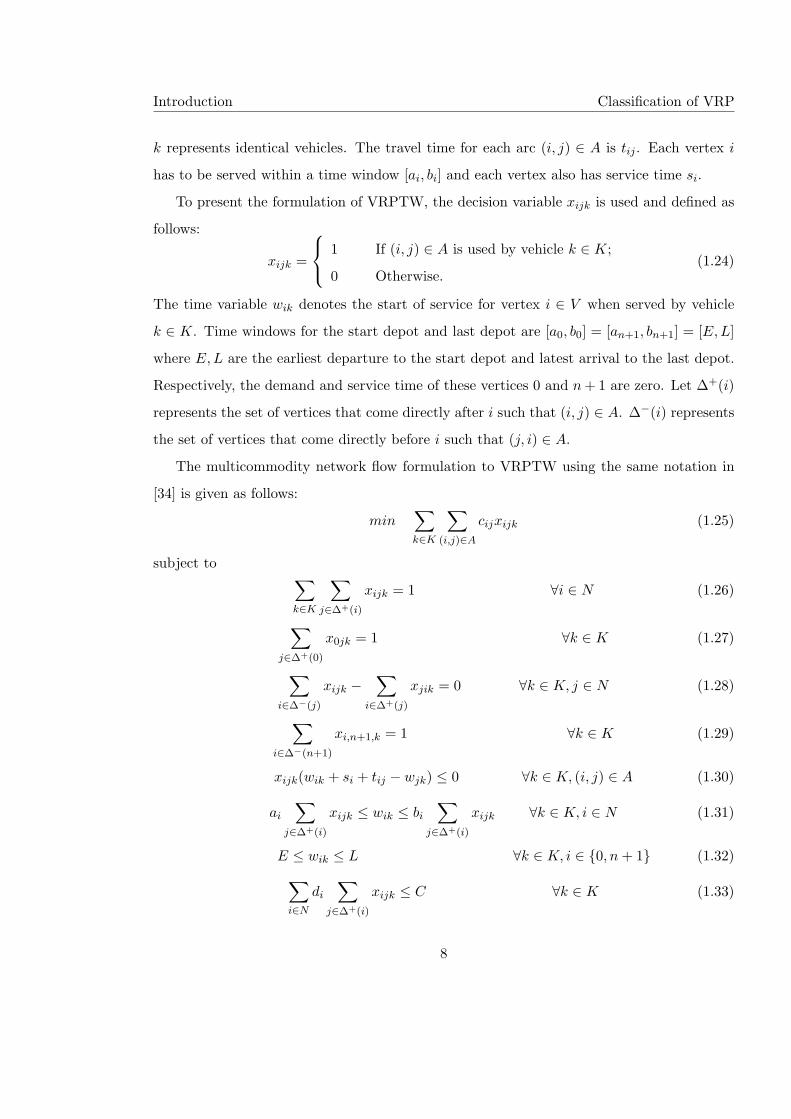
Let G = (V, A) be a complete directed graph, where V = {0, n+1}∪N and N = {1, ..., n}is a set of customers; 0, n + 1 represent the first and the last depot; A is the set of arcs; and
7
Introduction Classification of VRP
k represents identical vehicles. The travel time for each arc (i, j) ∈ A is tij . Each vertex i
has to be served within a time window [ai, bi] and each vertex also has service time si.
To present the formulation of VRPTW, the decision variable xijk is used and defined as
follows:
xijk =
1 If (i, j) ∈ A is used by vehicle k ∈ K;
0 Otherwise.(1.24)
The time variable wik denotes the start of service for vertex i ∈ V when served by vehicle
k ∈ K. Time windows for the start depot and last depot are [a0, b0] = [an+1, bn+1] = [E,L]
where E,L are the earliest departure to the start depot and latest arrival to the last depot.
Respectively, the demand and service time of these vertices 0 and n + 1 are zero. Let ∆+(i)
represents the set of vertices that come directly after i such that (i, j) ∈ A. ∆−(i) represents
the set of vertices that come directly before i such that (j, i) ∈ A.
The multicommodity network flow formulation to VRPTW using the same notation in
[34] is given as follows:
min∑
k∈K
∑
(i,j)∈A
cijxijk (1.25)
subject to∑
k∈K
∑
j∈∆+(i)
xijk = 1 ∀i ∈ N (1.26)
∑
j∈∆+(0)
x0jk = 1 ∀k ∈ K (1.27)
∑
i∈∆−(j)
xijk −∑
i∈∆+(j)
xjik = 0 ∀k ∈ K, j ∈ N (1.28)
∑
i∈∆−(n+1)
xi,n+1,k = 1 ∀k ∈ K (1.29)
xijk(wik + si + tij − wjk) ≤ 0 ∀k ∈ K, (i, j) ∈ A (1.30)
ai
∑
j∈∆+(i)
xijk ≤ wik ≤ bi
∑
j∈∆+(i)
xijk ∀k ∈ K, i ∈ N (1.31)
E ≤ wik ≤ L ∀k ∈ K, i ∈ {0, n + 1} (1.32)∑
i∈N
di
∑
j∈∆+(i)
xijk ≤ C ∀k ∈ K (1.33)
8
Introduction Classification of VRP
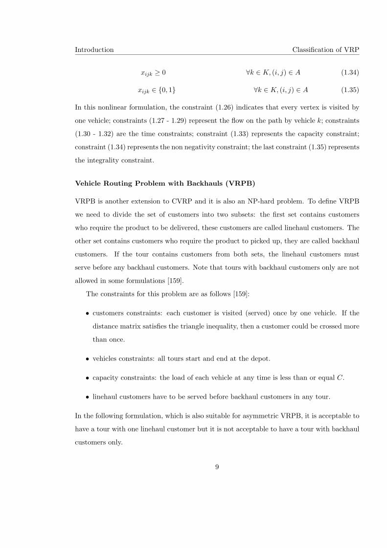
xijk ≥ 0 ∀k ∈ K, (i, j) ∈ A (1.34)
xijk ∈ {0, 1} ∀k ∈ K, (i, j) ∈ A (1.35)
In this nonlinear formulation, the constraint (1.26) indicates that every vertex is visited by
one vehicle; constraints (1.27 - 1.29) represent the flow on the path by vehicle k; constraints
(1.30 - 1.32) are the time constraints; constraint (1.33) represents the capacity constraint;
constraint (1.34) represents the non negativity constraint; the last constraint (1.35) represents
the integrality constraint.
Vehicle Routing Problem with Backhauls (VRPB)
VRPB is another extension to CVRP and it is also an NP-hard problem. To define VRPB
we need to divide the set of customers into two subsets: the first set contains customers
who require the product to be delivered, these customers are called linehaul customers. The
other set contains customers who require the product to picked up, they are called backhaul
customers. If the tour contains customers from both sets, the linehaul customers must
serve before any backhaul customers. Note that tours with backhaul customers only are not
allowed in some formulations [159].
The constraints for this problem are as follows [159]:
• customers constraints: each customer is visited (served) once by one vehicle. If the
distance matrix satisfies the triangle inequality, then a customer could be crossed more
than once.
• vehicles constraints: all tours start and end at the depot.
• capacity constraints: the load of each vehicle at any time is less than or equal C.
• linehaul customers have to be served before backhaul customers in any tour.
In the following formulation, which is also suitable for asymmetric VRPB, it is acceptable to
have a tour with one linehaul customer but it is not acceptable to have a tour with backhaul
customers only.
9
Introduction Classification of VRP
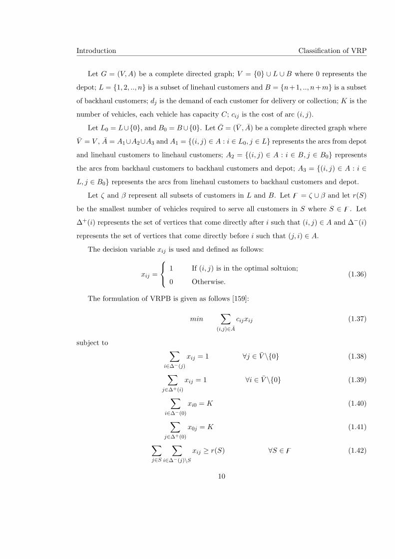
Let G = (V, A) be a complete directed graph; V = {0} ∪ L ∪ B where 0 represents the
depot; L = {1, 2, .., n} is a subset of linehaul customers and B = {n+1, .., n+m} is a subset
of backhaul customers; dj is the demand of each customer for delivery or collection; K is the
number of vehicles, each vehicle has capacity C; cij is the cost of arc (i, j).
Let L0 = L∪{0}, and B0 = B∪{0}. Let G = (V , A) be a complete directed graph where
V = V , A = A1∪A2∪A3 and A1 = {(i, j) ∈ A : i ∈ L0, j ∈ L} represents the arcs from depot
and linehaul customers to linehaul customers; A2 = {(i, j) ∈ A : i ∈ B, j ∈ B0} represents
the arcs from backhaul customers to backhaul customers and depot; A3 = {(i, j) ∈ A : i ∈L, j ∈ B0} represents the arcs from linehaul customers to backhaul customers and depot.
Let ζ and β represent all subsets of customers in L and B. Let z = ζ ∪ β and let r(S)
be the smallest number of vehicles required to serve all customers in S where S ∈ z. Let
∆+(i) represents the set of vertices that come directly after i such that (i, j) ∈ A and ∆−(i)
represents the set of vertices that come directly before i such that (j, i) ∈ A.
The decision variable xij is used and defined as follows:
xij =
1 If (i, j) is in the optimal soltuion;
0 Otherwise.(1.36)
The formulation of VRPB is given as follows [159]:
min∑
(i,j)∈A
cijxij (1.37)
subject to∑
i∈∆−(j)
xij = 1 ∀j ∈ V \{0} (1.38)
∑
j∈∆+(i)
xij = 1 ∀i ∈ V \{0} (1.39)
∑
i∈∆−(0)
xi0 = K (1.40)
∑
j∈∆+(0)
x0j = K (1.41)
∑
j∈S
∑
i∈∆−(j)\Sxij ≥ r(S) ∀S ∈ z (1.42)
10
Introduction Classification of VRP
∑
i∈S
∑
j∈∆+(i)\Sxij ≥ r(S) ∀S ∈ z (1.43)
xij ∈ {0, 1} ∀(i, j) ∈ A (1.44)
Constraints (1.38, 1.39) are the in-degree and out-degree for each customer, which means
that every customer is visited only once; constraints (1.40, 1.41) represent the in-degree
and out-degree of the depot; constraints (1.42, 1.43) represent the connectivity and capacity
constraints; the last constraint (1.44) represents the integrality constraint.
Vehicle Routing Problem with Pickup and Delivery (VRPPD)
VRPPD is an NP-hard problem. In the basic version of VRPPD, each customer i requests
two demands, di to be delivered and pi to be picked up. In addition, we need to add for each
customer i two new variables, Oi which denotes the vertex where the source of delivery exists
and Di which denotes the customer where the destination of the pick up exists. Assuming
at each customer the delivery is implemented before the pick up, so the constraints of the
basic VRPPD are as follows [43]:
• customers constraints: each customer is visited (served) once by one vehicle. If the
distance matrix satisfies the triangle inequality, then a customer could be crossed more
than once.
• vehicles constraints: all tours start and end at the depot.
• capacity constraints: The load of each vehicle must be less than or equal to Q and
should be satisfied all the time.
• each customer i must be served after the customer Oi and before customer Di in the
same tour in case both Oi and Di are not the depot.
Clearly, the customers who are required demand to be picked up only have to be served before
other customers including the customers who are required demand only to be delivered. The
formulation of VRPPD use three variables:
11
Introduction Classification of VRP
1. The time variable Tik determines the time when the service for customer i starts by
vehicle k.
2. The load variable Lik determines the load of vehicle k when the service for customer i
is finished.
3. The decision variable xijk is defined as follows:
xijk =
1 If (i, j) ∈ Ak is used by vehicle k ∈ K;
0 Otherwise.(1.45)
Let N = P ∪ D where P = {1, .., n} represents the set of pick up vertices, and D =
{n + 1, .., 2n} represents the set of delivery vertices. Assume vertex i requires demand di to
pick up and deliver to vertex n + i, let li = di and ln+i = −di.
Let K represents the set of vehicles, each vehicle with capacity Ck and serves a set of
vertices Nk = Pk ∪Dk where Nk, Pk, Dk are subsets of N, P, D. In addition, for each vehicle
there is a network Gk = (Vk, Ak) where Vk = Nk ∪ {o(k), d(k)} represents a set of vertices
including the source and destination depots for vehicle k. The travel time and cost between
two vertices using vehicle k is tijk and cijk respectively. The formulation of VRPPD is given
as follows [43]:
min∑
k∈K
∑
(i,j)∈Ak
cijkxijk (1.46)
subject to∑
k∈K
∑
j∈Nk∪{d(k)}xijk = 1 ∀i ∈ P (1.47)
∑
j∈Nk
xijk −∑
j∈Nk
xj,n+i,k = 0 ∀k ∈ K, i ∈ Pk (1.48)
∑
j∈Pk∪{d(k)}xo(k),j,k = 1 ∀k ∈ K (1.49)
∑
i∈Nk∪{o(k)}xijk −
∑
i∈Nk∪{d(k)}xjik = 0 ∀k ∈ K, j ∈ Nk (1.50)
∑
i∈Dk∪{o(k)}xi,d(k),k = 1 ∀k ∈ K (1.51)
12
Introduction Formulations
xijk(Tik + si + tijk − Tjk) ≤ 0 ∀k ∈ K, (i, j) ∈ Ak (1.52)
ai ≤ Tik ≤ bi ∀k ∈ K, i ∈ Vk (1.53)
Tik + ti,n+i,k ≤ Tn+i,k ∀k ∈ K, i ∈ Pk (1.54)
xijk(Lik + lj − Ljk) = 0 ∀k ∈ K, (i, j) ∈ Ak (1.55)
li ≤ Lik ≤ Ck ∀k ∈ K, i ∈ Pk (1.56)
0 ≤ Ln+i,k ≤ Ck − li ∀k ∈ K,n + i ∈ Dk (1.57)
Lo(k),k = 0 ∀k ∈ K (1.58)
xijk ≥ 0 ∀k ∈ K, (i, j) ∈ Ak (1.59)
xijk ∈ {0, 1} ∀k ∈ K, (i, j) ∈ Ak (1.60)
Constraints (1.47, 1.48) force each vertex requirement (pick up or delivery) to be served
once by the same vehicle; constraints (1.49 - 1.51) impose that each vehicle starts from its
origin depot o(k) and terminates at its destination depot d(k); nonlinear constraint (1.52)
is responsible for the suitability of the requirements between tours and schedules; constraint
(1.53) is the time window constraint where [ai, bi] is the time window interval for a vertex
i; constraint (1.54) forces each vehicle to visit the pick up vertex before the delivery vertex;
nonlinear constraint (1.55) is responsible for the suitability of the requirements between tours
and vehicle loads; constraints (1.56, 1.57) represent the vehicle capacity interval at the pick
up vertex and delivery vertex for each vehicle; constraint (1.58) represents the initial load for
each vehicle; the last constraints (1.59) and (1.60) are nonnegativity and binary constraints.
1.2 VRP Formulation Types
There are two types of integer programming formulations based on the constraints, [99]:
• polynomial size formulation: the number of constraints increase polynomially with the
number of vertices.
13
Introduction Formulations
• exponential size formulation: the number of constraints increase exponentially with
the number of vertices.
Polynomial size formulation can contain two types of formulations based on the type of
additional variables [99]:
• vertex based formulation: the additional variables are related to the vertices of the
graph.
• flow based formulation: the additional variables are related to the arcs of the graph.
There are three basic types of formulations used to represent VRPs [158]: vehicle flow
formulation; Commodity flow formulation; and set-partitioning formulation.
1.2.1 Vehicle Flow Formulation
In this formulation each arc or edge corresponds to an integer variable which represents how
many times this arc is used by a vehicle. Two-index vehicle flow formulation uses a variable
x(i, j) to represent whether arc (i, j) is used in the optimal solution or not. The three-index
vehicle flow formulation uses a variable x(i, j, k) to represent how many times the arc (i, j)
is used by vehicle k in the optimal solution, where the last index distinguishes between the
vehicles.
As an example we will present two-index vehicle flow formulation of CVRP as given in
[14] which was originally proposed by Laporte in 1985. Let G = (V,E) be an undirected
graph, V = {0} ∪N where N is the set of customers, m identical vehicles with capacity Q,
0 indicates to the central depot and E is the set of edges. Cij is the travel cost (or travel
distance) between vertex i and vertex j. The demand of vertex i is di where Q ≥ di ≥ 0 for
each i = 1, .., n and d0 = 0.
Let ϕ = {S : S ⊆ V \{0}, |S| ≥ 2} and let S = V \S be the complementary set of S.
Assume d(S) =∑
i∈S di is the whole demand of the vertices in S, k(S) is the minimum
number of vehicles required to serve all vertices in S.
14
Introduction Formulations
Let xij be an integer variable defined as follows:
xij =
2 If i = 0 and route with one vertex exists in the solution;
1 If {i, j} belongs to an optimal solution where (i 6= 0 and j 6= 0)
or (i = 0 and j 6= 0);
0 Otherwise.
(1.61)
The two-index vehicle flow formulation for CVRP is as follows:
min∑
{i,j}∈E
cijxij (1.62)
subject to:∑
j∈V,i<j
xij +∑
j∈V,i>j
xji = 2 ∀i ∈ N (1.63)
∑
i∈S
∑
j∈S,i<j
xij +∑
i∈S
∑
j∈S,i<j
xij ≥ 2k(S) ∀S ∈ ϕ (1.64)
∑
j∈N
x0j = 2m (1.65)
xij ∈ {0, 1, 2} ∀{i, j} ∈ E (1.66)
The constraint (1.63) represents the degree of each vertex (each vertex that is served); con-
straint (1.64) represents the capacity constraint (subtour elimination constraint); constraint
(1.65) represents the depot degree (m vehicles leave and m vehicles return to the depot);
and finally constraint (1.66) is integrality constraint.
1.2.2 Commodity Flow Formulation
This formulation was proposed originally by Garvin et. al in 1957 (see [52]). It requires two
continuous variables to be connected with each arc (or edge). These continuous variables
represent the flow of commodities on the arcs (or edges) used by the vehicles in the tour.
In other words, commodity flow formulation requires two flow variables yij and yji, both
represent the load of vehicles of a feasible solution in two sides. Suppose the vehicle travels
from vertex i to vertex j then yij denotes the load of the vehicle, while yji denotes the empty
15
Introduction Formulations
space in the vehicle, where yij +yji = Q (vehicle capacity). This has to satisfied for all routes
in the feasible solution.
Another copy of the depot has to be added. There are one, two, and multi-commodity
flow formulations. Any route in a feasible solution to CVRP has two paths, the first path
from the depot 0 to the depot (n + 1) and uses yij , while the second path starts from the
depot (n + 1) to the depot 0 and uses yji. Let d(N) denotes to the demand of all vertices.
Let S = V \S be the complement of S where S ⊆ V \{0}. This formulation needs to add
one vertex n+1 as a copy of the depot 0 to the graph. Therefore, the extended graph contains
two depots and it is denoted by G = (V , E) where V = V ∪ {n + 1}, N = V \{0, n + 1}, and
E is given: E = E ∪ {{i, n + 1}|i ∈ N}, cin+1 = c0i where i ∈ N .
In this formulation xij is a binary variable defined as follows:
xij =
1 If {i, j} ∈ E belongs to the optimal solution ;
0 Otherwise.(1.67)
The two commodity flow formulation for CV RP which was proposed by Baldacci in 2004
(see [14]) is as follows:
min∑
{i,j}∈E
cijxij (1.68)
subject to:∑
j∈V
(yji − yij) = 2di ∀i ∈ N (1.69)
∑
j∈N
y0j = d(N) (1.70)
∑
j∈N
yj0 = mQ− d(N) (1.71)
∑
j∈N
yn+1j = mQ (1.72)
∑
j∈V ,i<j
xij +∑
j∈V ,i>j
xji = 2 ∀i ∈ N (1.73)
yij + yji = Qxij ∀{i, j} ∈ E (1.74)
yij ≥ 0, yji ≥ 0 ∀{i, j} ∈ E (1.75)
16
Introduction Formulations
xij ∈ {0, 1} ∀{i, j} ∈ E (1.76)
The constraint (1.69) represents the difference between the inflow and the outflow for each
vertex which is equal to the double of the demand of that vertex. Constraint (1.70) shows that
the outflow at the depot 0 is equal to the demand of all vertices. Constraint (1.71) indicates
the inflow at the depot 0 which is equal to the difference between the vehicle capacity and
the total vertices demand. Constraint (1.72) represents the outflow at the depot (n+1) to be
equal to the total capacity of all vehicles. Constraint (1.73) forces the degree of each vertex to
be 2. Constraint (1.74) defines the edges of a feasible solution. Finally, the constraint (1.75)
represents the non-negative constraint and the constraint (1.76) is the integrality constraint.
1.2.3 Set-Partitioning Formulation
This formulation was proposed in 1964 by Balinski and Quandt (see [18]) with the model
containing an exponential number of binary variables. It is necessary to define one variable
for every feasible tour that is used by a single vehicle [121], so that when the size of the
problem increases polynomially, the number of variables grows exponentially. For this reason
using column generation becomes necessary [121]. In addition, this formulation needs a huge
number of variables.
Let R be the set of all possible routes, each route has cost cl corresponding to the sum
of costs of edges in that route, xl is a binary variable defined as follows:
xl =
1 If route l ∈ R belongs to an optimal solution;
0 Otherwise.(1.77)
ail is a binary coefficient defined as follows:
ail =
1 If vertex i ∈ V belongs to route l ∈ R;
0 Otherwise.(1.78)
The Set-Partitioning formulation of CVRP is as follows [121]:
min∑
l∈R
clxl (1.79)
17
Introduction ADVRP
subject to:∑
l∈R
xl = m (1.80)
∑
l∈R
ailxl = 1 ∀i ∈ V (1.81)
xl ∈ {0, 1} ∀l ∈ R (1.82)
The constraint (1.80) shows that m routes are chosen, constraints (1.81) shows that each
vertex has to be on one route. The final constraint (1.82) is integrality constraint. If
the distance matrix satisfies the triangle inequality, then set partitioning formulation is
transformed to set covering formulation [26].
1.3 Distance-Constrained Vehicle Routing Problem
In general if we relax the distance constraints from DVRP, then it will become M-TSP. In
addition, if there is only one vehicle then DVRP will become TSP [108]. Solving TSP or M-
TSP is easier than solving VRPs [108]. A real world application can be sales representative
visits customers without pick up or delivery requirements but with distance constraints [108].
1.3.1 History
The literature is rich for symmetric VRPs and poor for asymmetric VRPs, although the
symmetric VRPs is considered as a special case of asymmetric VRPs. The exact methods of
asymmetric VRPs have a weak performance on symmetric VRPs. Furthermore, the methods
designed for symmetric VRP instances may not be adapted easily to solve asymmetric VRPs
[70].
Surprisingly, ADVRP is not studied like other types of VRPs. There are a few papers
that discuss this problem see [99, 113].
• The first paper was in 1984 by Laporte, Desrochers and Nobert [108]. It presents two
exact algorithms for DVRP. One of them is based on Gomory cutting planes and the
other one is based on branch and bound. They deal with symmetric instances (Eu-
clidean and non-Euclidean) where Euclidean means that the distance matrix satisfies
18
Introduction ADVRP
the triangle inequality. They conclude that solving non-Euclidean instances is easier
than solving Euclidean, where both algorithms are able to find the optimal solution
with up to 50 customers in Euclidean cases and 60 in non-Euclidean instances. In
addition, the cutting plane algorithm performs better than branch and bound algo-
rithm. Moreover, in both algorithms, solving instances become more difficult when the
maximum distance allowed is decreased.
• Laporte, Nobert and Desrochers in 1985 present an integer linear programming al-
gorithm to solve VRP with distance and capacity constraints. They use relaxation
constraints and subtour elimination constraints. They solve the model with up to 60
customers [112] using Euclidean and non-Euclidean instances.
• The third paper was in 1987 by Laporte et. al [113]. It is considered as the first
paper with Asymmetric DVRP in the operations research literature. They use similar
techniques to Laporte et. al (see [110]) which is originally considered as an extension
to the algorithm of Carpaneto and Toth for TSP [28].
An exact algorithm for solving ADVRP is developed in [113]. It uses the branch and
bound method where the relaxation problem is the modified assignment problem. They
extend the distance matrix based on the technique of Lenstra and Rinnooy (see [120])
by adding (m − 1) dummy depots where m represents the number of vehicles. The
solution is feasible to ADVRP if two conditions are satisfied:
– the solution contains m hamiltonian circuits.
– the length for each of them is less than or equal to the maximum distance allowed.
In the case that the infeasible solution is obtained, the infeasible circuit is eliminated
by adding a new constraint. This means the illegal subtour is eliminated by branching
this infeasible subproblem into subproblems.
They find the first feasible solution by adapting Clarke and Wright’s algorithm (see
[32]). If this is not able to provide a feasible solution then the upper bound (UB) is
set to: UB = m × Dmax where Dmax represents the maximum distance allowed. If
19
Introduction ADVRP
the total length of a subtour is greater than Dmax, then it has to be eliminated. They
eliminate illegal tours by excluding arcs.
They use randomly generated instances, with two types of distance matrices, those
satisfying and not satisfying the triangle inequality. This method is able to solve up to
100 customer problems for ADVRP. They conclude that solving tighter problems are
more difficult.
• The forth paper published in 1992 by Li et. al, see [122], considers two objective func-
tions to DVRP: minimize total distance and minimize the number of vehicles used.
They transform the DVRP into a multiple traveling salesman problem with time win-
dows (mTSPTW), where the time window constraint [ai, bi] for any customer i means
that it is not allowed to serve customer i before ai or after bi. In other words, the
vehicle has to wait until time ai to start before dealing with customer i. For details on
time windows with VRP see Section 1.1.
In order to enable the transformation, the distance constraint is used as a time window
constraint [0, Dmax] for all customers, and another copy of the depot is added to the
graph. The time window for the first depot is [0, 0] (departure depot), and the time
window for the last depot is [0, Dmax] (arrival depot). It is solved using a column
generation approach. They present and analyze the worst case performance for DVRP
with a heuristic and provide results with up to 100 customers. The comparison includes
the length of the initial tour and the value of the lower bound.
• Conference paper by Almoustafa et.al in 2009 [7]. An old branch-and-bound method
(suggested by Laporte et al. in 1987) is revised and modified. This method is based on
reformulating the distance–constrained vehicle routing problem into a traveling sales-
man problem and use of the assignment problem (AP) as a lower bounding procedure.
The Hungarian algorithm is used to find the solution to AP (an efficient implementa-
tion of Hungarian method for AP). In [7] branching based on tolerances and costs are
used in two algorithms.
Computational results indicate that according to how many times the optimal solution
20
Introduction ADVRP
is found, the performance of tolerance-based algorithms is better than the performance
of cost-based algorithms. On the other hand, the opposite is held when the CPU time
is considered. Both algorithms are able to find optimal solution up to 200 customers.
• Kara emphasized in 2011 that there are still a limited number of published papers on
DVRP in this area of literature [98, 99, 100]. Kara’s technical report [99] displayed the
existing formulations and presented new formulations for DVRP:
– flow based formulation.
– vertex based formulation.
All new formulations have O(n2) binary variables and O(n2) constraints and it can
be used by commercial solvers such as CPLEX. The flow based formulation performs
better than vertex based formulation according to the computational times. On the
other hand, the vertex based formulation provides better lower bounds than flow based
formulation [98].
Kara recommends flow based formulation to solve small and moderate-sized cases, while
vertex based formulation to be used to improve heuristic procedures for DVRP [98].
Finally the proposed formulations by Kara can be adapted by adding other constraints
to DVRP.
1.3.2 Our Approach
Our target is to increase the size of instances that can be solved exactly by our approach to
solve ADVRP. In addition, our target is to propose a simple and robust algorithm. In this
thesis we propose three results.
Firstly, we present a general flow-based formulation to solve ADVRP. This formulation
is more general than Kara formulation [98], since it does not require the distance matrix to
satisfy the triangle inequality. It produces a solution faster than the adapted formulation.
In addition, we are able to improve the quality of the objective function in case the optimal
solution is not reached because of stopping conditions.
21
Introduction Thesis Overview
Secondly, we use tolerance based branching rules [6] and try to improve it in different
ways. First of all by using CPLEX as a lower bounding procedure to solve AP and comparing
that with the Hungarian algorithm. We find that the Hungarian algorithm produces a
solution in shorter CPU time when compared with CPLEX for solving AP. In other words,
there is a big gap, in terms of time, between using the Hungarian algorithm and CPLEX to
solve AP.
Tolerance based branching rules method is fast but memory consuming, and could stop
before optimality is proven. Therefore, we introduce randomness in choosing the node of the
search tree in cases where we have more than one choice. If an optimal solution is not found
and restart is required due to memory issues, we restart our procedure. In this way, we get
a multistart branch and bound method.
Computational experiments show that we are able to exactly solve large test instances
with up to 1000 customers. So, despite the simplicity, this proposed algorithm is capable of
solving the largest instances ever solved in literature. As far as we know, those instances are
much larger than instances considered for other VRP models and exact solution approaches
from recent literature. For example CVRP is not always able to solve instances optimally
with more than 200 customers [48].
In order to compare our approach we use a commercial IP solver (CPLEX) to get the
optimal solution of the ADVRP. Using CPLEX solver to obtain the optimal solution to
ADVRP faces some difficulties for two reasons. The first reason is related to the CPU time
which is too long and the second reason is related to the larger instances which can’t be
uploaded due to lack of memory.
Thirdly, we develop heuristic based on VNS to find a good feasible solution in case our
exact multistart branch and bound method stops because of memory or stopping conditions.
We use the route-first-cluster-second approach to transfer TSP solution to ADVRP solution.
Unsatisfactory results are obtained. The reason for not getting expected good results could
be the route-first-cluster-second approach.
22
Introduction Thesis Overview
1.4 Thesis Overview
The structure of this thesis is as follows:
• Chapter 1 we present classification of VRPs based on constraints (unconstrained VRP
and constrained VRP), then we explain in more detail definitions and formulations of
the main constrained VRPs: Capacitated VRP; distance-constrained VRP; VRP with
time windows; VRP with backhauls; and VRP with pickup and delivery. In addition,
basic formulation types for VRPs are presented.
• Chapter 2 we provide basic information about the solution methods: Exact methods
that find the optimal solution such as: branch and bound, cutting plane, branch and
cut, column generation, cut and solve; branch-and-cut-and-price, branch-and-price,
and dynamic programming; Classical Heuristics that find approximate solution such
as: constructive heuristics, two phase methods, improvement heuristics; Metaheuristics
are classified into three groups, and are presented with basic information as follows:
1. Local search based metaheuristics: such as multi-start method, simulated an-
nealing (SA), tabu search (TS), greedy randomized adaptive search procedure
(GRASP), neural networks (NN), variable neighborhood search (VNS), and guided
local search (GLS).
2. Population Based (natural inspired): genetic algorithm (GA), evolutionary al-
gorithm (EA), scatter search (SS), Ant colony optimization (ACO), and Path
Relinking (PR).
3. Hybrid metaheuristics.
In addition, we provide more information on VNS, since it is used in Chapter 5 to find
feasible solutions to ADVRP. We propose different variants of VNS types and their
algorithms.
• Chapter 3 we present three formulations for ADVRP: adapted bus school routing prob-
lem (ABSRP), Kara formulation, and our general formulation. We explain the differ-
ence between Kara formulation and our general formulation then we compare between
23
Introduction Thesis Overview
adapted formulation and our general formulation with an illustrative example. Finally,
we present computational results and the conclusion.
• Chapter 4 Multistart Branch and Bound for ADVRP (MSBB− ADVRP): a simple intro-
duction is presented in section 4.1, then mathematical programming formulations of
ADVRP is in section 4.2. We discuss in section 4.3 single start branch and bound for
ADVRP and most of the relevant basic concepts which are used later: upper bound,
lower bound, branching rules, the algorithm, and an illustrative example. A descrip-
tion of the multi start method used to solve ADVRP is given in section 4.4 with the
algorithm and an example. An efficient implementation and data structure are given in
section 4.5. Computational results are provided in section 4.6 with methods compared,
numerical analysis and summary tables of results. Section 4.7 contains the conclusion
and future research directions. For more information on the detailed tables of results
see Appendix A.
• Chapter 5 Variable neighborhood search (VNS), we explain our VNS based heuristic
for solving ADVRP. The initialization algorithms are presented in section 5.1, and the
main algorithm VNS-ADVRP is explained with more detail in section 5.2 and illustrated
with an example. The last two sections present the obtained results and the analysis
beyond them, conclusion and future research. For more information on the detailed
tables of results see Appendix B.
• Chapter 6 contains a summary of thesis conclusions and possible future research where
we suggest some ideas for further research.
• Appendix A contains tables of results for Multistart Branch and Bound for ADVRP
in Chapter 4.
• Appendix B contains tables of results for Variable Neighborhood Search in Chapter 5.
24
Chapter 2
Solution Methods
Three types of algorithms are used to solve any VRP:
• Exact algorithms which look for an optimal solution. Such methods include branch
and bound, cutting plane, branch and cut, column generation, cut and solve, branch-
and-cut-and-price, branch-and-price, and dynamic programming.
• Classical heuristics which search for a good feasible solution without guarantee of opti-
mality. Such methods include constructive heuristics, two phase methods, improvement
heuristics.
• Metaheuristics or framework for building heuristics. They are classified in this the-
sis into three groups: local search based metaheuristics, population based (natural
inspired), and hybrid metaheuristics.
For surveys of solution methods for VRPs we refer to [49, 106, 111, 114, 160].
2.1 Exact Algorithms
These type of methods are able to find an optimal solution to any instance with a proof
of optimality [144]. This has been studied by many authors [16, 31, 106, 111, 120]. When
the size of the problem increases polynomially, the CPU time which is required to solve the
problem increases exponentially [144]. We will explain some of these exact methods:
25
Solution Methods Exact Algorithms
2.1.1 Branch and Bound (B&B)
B&B was introduced in 1960s and usually used to solve discrete optimization problems
defined as an integer program, and it has been used as an exact method to solve most
types of VRPs. The B&B uses a relaxation of the original problem. The most important
components in B&B are:
• The quality of the bounds (upper bound (UB) and lower bound (LB)): UB is the value
of the best feasible solution found so far and it is called incumbent. LB is the value of
the objective function to the current node, which is not possible to reach any successor
node with smaller value than LB in case the current node is expanded further. When
a good UB is found early in the search tree, pruning becomes more effective.
• The search strategy: it defines how the next node is chosen for branching. There are
three basic strategies [128]:
1. Breadth first search: Expand the search tree by one level, then examine all nodes
in this level before the next level is expanded until the solution is found. It is not
possible to solve large problems using this strategy because the number of nodes
in the search tree increases exponentially at each level.
2. Depth first search: Expand the search tree by choosing the last generated node
and continue until you find a solution or you find a node without children, then
backtrack to the recent generated node which is not explored yet. It requires
polynomial memory space but the solution times and the search tree are large.
Finding a good upper bound will be useful in this strategy to reduce the size of the
search tree by fathoming large numbers of nodes since their lower bound values
are greater than the values of the upper bounds.
The negative point of this strategy appears when the value of the incumbent is not
close to the value of the optimal solution, which means unnecessary computations
could be made with undesirable extra CPU times. According to the observation
in [124] this search strategy performs weakly in practice even if a heuristic is used
to find an initial solution.
26
Solution Methods Exact Algorithms
3. Hybrid search: Suppose a minimization problem. The hybrid search strategy
chooses the node with the smallest lower bound to branch and it is a good strategy
in minimizing the total number of nodes in the search tree, which have to be
explored before the optimal solution is found [144]. This strategy focuses on
looking for proof of optimality, which means that there is no solution better than
the incumbent [124]. This is also known as best first search strategy.
Best first search strategy is the fastest but it requires exponential memory space.
It is considered more efficient than breadth first search because it branches less
subproblems [170]. However, compared with the depth first search, it is less
affected by using an initial upper bound.
In this thesis we use the best first search strategy because it is the fastest and
we expect it to be useful in solving larger instances. However, we are not using
any heuristic to find an initial upper bound because there will be no observable
benefit based on the fact that B&B is able to find a feasible solution early in the
search tree [47].
The search tree initially contains a root node which represents the original problem. During
the search it will be increased by adding new nodes. All other nodes in the search tree
represent subproblems, where every new generated node is numbered. At each iteration, a
node from a list of active nodes (unexplored nodes) is chosen based on the search strategy
to expand. Each new node is checked. If it produces a feasible solution then the value of the
upper bound is updated. Otherwise, the node produces an unfeasible solution. Once again,
if its value is larger than the current incumbent then it will be fathomed. If not, then it will
be added to the list of active nodes to be expanded further during the search.
The new generated nodes (children) are tightened more than parent nodes because they
have more constraints. Relaxation of the original problem is solved at each node in the
search tree. Fathoming (or pruning) is an important feature of the B&B tree in helping to
minimize the number of generated nodes in the search tree.
The search in any branch will stop in one of these cases: a feasible solution is found, or
the value of the objective function is worse than the value of the UB (best feasible solution
27
Solution Methods Exact Algorithms
found so far) [166]. When there are no more unexplored nodes in the search tree, the search
in the whole B&B tree terminates and the optimal solution (if it exists) is the value of the
current upper bound.
When B&B procedure is used for solving a problem, we have to decide [13]:
• what constraints to relax? (in order to solve the problem easily).
• what branching rules to use? (a rule to split the feasible set to subsets).
• what lower bounding procedure to be used? (it is a procedure to find the value of the
objective function for the relaxation problem at each subproblem).
• what search strategy to be used? (it is a rule to choose the next subproblem to be
processed).
• what upper bounding procedure will be used?
• how to fathom? and when to stop?.
The initial (good) feasible solution is usually obtained by heuristic. The value obtained is
used as the initial UB, which helps fathoming nodes and reduces the size of the search tree.
If there is no known heuristic solution then the upper bound UB = ∞.
Relaxation in general means some or all constraints are dropped. There are two kinds of
relaxations: basic combinatorial relaxation and sophisticated relaxation, such as Lagrangian
relaxation [157]. Lagrangian relaxation is defined as taking some constraints out and adding
them to the objective function [166]. It provides tight lower bounds but demands more
computational time. To have a relaxed model that is easier to solve, you are recommended
to choose difficult constraints (complicating constraints) to relax and add to the objective
function [166].
The effectiveness of B&B is based on the strategy used to choose the next node in the
search tree to branch [3]. In addition, it is based on the quality of the upper bounds that
are used to minimize the size of the search tree [13]. In other words, to keep the B&B tree
small, a good upper bound is required [144]. In order to get a good upper bound, you need
28
Solution Methods Exact Algorithms
to apply heuristic or metaheuristic at some nodes in the search tree [144]. Therefore, the
efficiency of B&B is based on the rapid convergence of the lower and upper bounds [124].
There are two methods to improve the B&B algorithm [70]:
• tight the bounds: enlarge lower bound or use heuristic to get good upper bound.
• improve the branching rules: use different branching rules to improve the algorithm.
Note that a feasible solution is often found early in the B & B search tree but the
confirmation of optimality requires longer CPU time to be proved [47]. In addition, B&B
can be used as heuristic to produce feasible solutions during a given time [47].
Survey of Branch and Bound
B&B algorithm is one of the most successful methods to solve MIPs. It is based on two
principles, branching and selecting the node from the search tree. There are several types of
branching such as (for more information see [3]):
• Most infeasible branching: it is not good enough because its results are similar to
random branching.
• Pseudocost branching: it is effective but not strong at the beginning.
• Strong branching: it is effective if evaluated based on the number of nodes in the
search tree, while it is inefficient if evaluated based on time [3]. In case the full set of
candidates is used, it is called full strong branching.
• Reliability branching: it is a generalization of pseudocost and strong branching, and
its performances are better than hybrid strong/pseudocost branching.
Our branching rules, which are based on tolerances, are similar to strong branching.
Strong branching proposed in CPLEX 7.5 checks the candidates (fractional variables) to
calculate the extra cost of giving an integer value to a fractional variable in order to decide
which variable to choose for branching [3]. Tolerance calculates the extra cost of removing
the infeasibility of the current solution (destroying an infeasible tour by removing one arc)
before selecting which subproblem to develop further.
29
Solution Methods Exact Algorithms
2.1.2 Cutting Planes
This technique is used when there is a large number of linear constraints of IP, or when
the linear relaxation becomes stronger by adding some valid inequalities [137]. It generates
Gomory Cuts [166]. Gomory cuts are used to tighten the relaxed problem by deleting part
of the solution space [73]. The added cuts will not affect the original problem but will affect
the relaxed problem by increasing the chance of finding a solution. The method should be
applied as follows: Add cuts then solve the relaxation problem, continue until the solution
at the current relaxation problem equals the incumbent (current upper bound), then stop
with the value of the incumbent as the optimal solution [73].
2.1.3 Branch and Cut (B&C)
It is an incorporation of the branch and bound algorithm and cutting plane method. Cutting
plane can be applied at the root node (global cuts) or at every node (local cuts) in the search
tree. This will produce a smaller sized tree (i.e. reduce the size tree) [129, 166]. B&C adds
cutting plane to a tight relaxed subproblem by deleting a set of solutions for the relaxed
subproblem. The deleted solutions are not feasible to the unrelaxed subproblem [90].
The positive point of B&C is that it reduces the size of the search tree which helps to
increase the size of solvable instances, while the negative point is that it increases the time
at each node in the search tree [90]. In branch and cut the enumeration benefits from cutting
plane, where the lower bound obtained from the enumeration tree is better than the bound
obtained from the branch and bound tree [137]. On the other hand, cutting plane benefits
from enumeration, where the separation algorithm can be more active when it is used with
branching [137].
2.1.4 Other Approaches
In the literature there are also exact methods such as:
• Cut and Solve: Cut and Solve uses a path tree instead of search tree. It solves two
easy subproblems at each node: a relaxed problem and a spare problem, and it adds a
30
Solution Methods Classical Heuristics
constraint to a relaxed problem. The positive points of this method are that the search
will not choose the wrong branch because it has only one branch, and the memory
requirements are reasonable [33].
• Column Generation: This technique adds more variables to the problem in order to
avoid increasing the number of constraints [166]. It is considered as a dual of cutting
plane [144]. For example in [29] the original linear program is divided into a linear
restricted master problem and a pricing subproblem. For more details on column
generation we refer to [44, 74, 118].
• Branch-and-Cut-and-Price: It is defined as a combination of B&B, cutting plane
method and column generation, and produces influential algorithms [51, 144].
• Branch-and-Price: It is defined as a combination of B&B and column generation. New
columns are generated at each node from the search tree [144].
• Dynamic Programming: Dynamic programming was proposed by Bellman [22]. It is a
procedure used to solve optimization problems, and is also called multistage program-
ming [47]. Dynamic programming has four elements: stages, states, decisions, and
policies [47].
2.2 Classical Heuristics
Not all problems can be solved by exact method for many reasons. For example, if a problem
has a large number of constraints, or a huge search space, then the number of feasible
solutions will be enormous, so it will be difficult to find the optimal solution [128]. As we
mentioned before VRP is an NP hard problem, for this reason it can sometimes be difficult to
find the optimal solution during an acceptable computational time even for small instances.
Consequently we have to accept the best feasible solution that is found in a reasonable
computational time, rather than concentrate on finding the optimal solution [102]. Therefore,
we need to use other methods such as heuristics or metaheuristics.
31
Solution Methods Classical Heuristics
Heuristics have been studied by many researchers [32, 116, 160] and developed between
1960 and 1990 [109]. It is defined as techniques to find approximate solution, namely a
procedure which produces a good feasible solution (not optimal) [89]. This produces an
approximate solution, but without guarantee of optimality. Heuristics such as local search
can find near optimal solutions in reasonable running times. It begins with an initial solution
trying to search in its neighborhood to find a solution that is better than the current one.
This will continue until no better solution is found, then local search will stop presenting the
current solution as locally optimal. Empirical results emphasize that local search is able to
find acceptable solutions in acceptable CPU times [1].
The effectiveness of heuristics is measured by the running time (CPU) and the quality
of the solution, which is measured by calculating the ratio between the value of the final
solution obtained by the heuristic and the optimal solution or best known feasible solution
obtained from the literature [1].
According to [35] heuristics can be compared using four criteria: accuracy, speed, sim-
plicity and flexibility. They report the best known heuristics for VRP: Clarke and Wright’s
algorithm [32] is one of the best known algorithm in the last decade because of its simplicity
and speed [35], the Sweep algorithm (less simple, more speedy) [61], and Fisher and Jaiku-
mar algorithm [50]. Greedy algorithm is popular because it is simple, easy and fast but it is
not sufficient [128].
The weakness of heuristics is that each heuristic is designed for a specific problem [128].
Some of the traveling salesman problem heuristics may be used with minor modifications for
solving VRP such as: nearest neighbor heuristic, insertion heuristic, and tour improvement
heuristic. Besides these there are many other heuristics [106].
In [102] they consider heuristics with two stages, the first is called construction stage
and builds an initial solution; the second is called local search stage and develops the initial
solution by searching the neighborhood. In this thesis, based on [115], the classical heuristics
are divided into three groups as follows: constructive heuristics; two phase methods; and
Improvement heuristics.
32
Solution Methods Metaheuristic
2.2.1 Constructive Heuristics
These heuristics focus on constructing a feasible solution with a main interest on the cost
and not improvement [115]. There are two main techniques used to construct a feasible solu-
tion. The first technique is insertion heuristics, which constructs a solution by inserting one
customer each time. Greedy algorithms are a good example of this class, it uses construction
to get feasible solutions [128]. The second technique is savings heuristics, which uses the
idea of merging the routes where each customer is served.
As an example is Clark and Wright Savings Algorithm [32].
2.2.2 Two Phase Methods
Two models exist: first is cluster-first, route-second: cluster the vertices to get feasible
clusters then construct a feasible route for each cluster. In other words, gather the customers
into subsets, then build a route for each subset e.g Fisher and Jaikumar algorithm [50]. The
second model is route-first, cluster-second: construct one route for all vertices then separate
it into feasible routes (see [19]).
This type of heuristics provide good quality feasible solutions compared with constructive
heuristics [115].
2.2.3 Improvement Heuristics (Local Search)
The search starts from any initial feasible solution and attempts to improve it in the neigh-
borhood of the initial solution. The improvement can be exchanging an arc or a vertex in a
route or exchanging between the routes [115].
2.3 Metaheuristics
Metaheuristics are considered a powerful approach applied to difficult combinatorial opti-
mization problems and achieve great results [57]. It consists of heuristics that are based on
some metaheuristic rules.
33
Solution Methods Metaheuristic
The motivation behind metaheuristics is to explore the search space in an effective and
efficient way [25]. Such metaheuristics (or framework for building heuristics) are Multi-
start local search [125, 126], Simulated annealing [2, 89, 128, 138], Tabu search [12, 54, 88,
162], Greedy randomized adaptive search procedure [151], Neural networks [128], Variable
neighborhood search [85], Guided local search [164], Genetic algorithms [41, 160], Scatter
search [65], Ant colony optimization [46], Evolutionary algorithm [25], Path relinking [65],
etc. For more information on the best known metaheuristics and some of their applications
see these books [58, 63, 146].
Metaheuristic methods combine sophisticated rules in a neighborhood search, the struc-
ture of memory, and recombination of solutions. By this combination metaheuristics aim
to improve the quality of solutions compared with classical heuristics but with higher com-
puting time [109]. In addition, metaheuristics use different methods to escape from local
optima such as iterate local search (Multistart local search, GRASP), change the neighbor-
hood (VNS), move to non-improving neighbors (TS, SA). For an overview of metaheuristics
see [55, 140] and for developments in the field of metaheuristics applied to VRP see [23, 57].
Local search indicates that there is a relationship between the effectiveness of the search
and the search space [128]:
• If the search space is chosen to be small then the search will finish quickly and the
local optimum will be found. In this case the quality of the optimum solution is poor.
It is recommended to increase the search space in order to improve the quality of the
solution.
• If the search space is large then we would not complete the search because of time,
memory or anything else.
For such reasons the search space should not be established randomly [128]. Metaheuristics
can be compared based on the following principles [83]:
1. Simplicity: simple to implement, to explain, or to analyze.
2. Coherence: the steps of heuristics for a specific problem should logically follow the
metaheuristic’s rule.
34
Solution Methods Metaheuristic
3. Effectiveness in finding optimal or near optimal.
4. Efficiency in finding a good (or an approximate) solution in a reasonable CPU time.
5. Robustness for different instances not only for specific instances.
6. User-friendliness: the metaheuristics are preferred to be easy to understand and easy
to implement, which requires the metaheuristics to have just a few parameters.
7. Generality: this means they have to be suitable for several types of problems.
8. Interactivity by allowing the user to improve the process.
9. Multiplicity: the ability to present some near optimal solutions.
For more details on how to compare metaheuristics we refer to [155]. There are several types
of classification such as nature-inspired (ACO) vs non-nature inspired metaheuristics (TS)
[25]; constructive versus iterative; deterministic versus stochastic; memory usage (TS, GA)
versus no-memory (SA).
Metaheuristics classified in this thesis based on the number of solutions used by a meta-
heuristic at any time as follows:
1. Local Search Based Metaheuristics: this class of metaheuristics use one solution to
get another. For example, simulated annealing (SA), tabu search (TS), determinis-
tic annealing (DA), greedy randomized adaptive search procedure (GRASP), neural
networks (NN), variable neighborhood search (VNS), guided local search (GLS), and
iterated local search (ILS).
The stopping conditions for most of them can be maximum CPU time, maximum
number of iterations, or maximum number of iterations without improvement [25].
2. Population Based (natural inspired): This uses more than one solution to find a new
solution. For example, genetic algorithm (GA), evolutionary algorithm (EA), scatter
search (SS), ant colony optimization (ACO), particle swarm optimization (PSO), and
Path relinking (PR).
35
Solution Methods Metaheuristic
3. Hybrid Metaheuristics: The combination between metaheuristics and the techniques
of optimization (Artificial intelligence (AI) and Operation research (OR)) is known as
hybrid metaheuristic and it produces efficient results [25].
2.3.1 Local Search Based Metaheuristics
Multi-start Local Search
Multi-start procedure is designed to diversify the search and to escape local optima [125].
The method has two stages: first stage generates a solution and second stage improves it
[126]. The output of Multi-start algorithm is the best local optima found [126].
The classification of Multi-start methods can be based on one of these factors: memory
(use memory or memoryless), randomization (systematic or randomized), degree of rebuild
(built from scratch or fix some elements in the previous generated solutions) [126].
The main steps of Multi-start algorithm is as follows [125]:
• first iteration i = 1;
• while stopping condition is not satisfied do
– construct solution si;
– improve the solution si to get s′i;
– update the best solution found so far;
– i = i + 1;
Simulated Annealing (SA)
SA is well studied in literature [138]. It provides a method to avoid the local optimum in
order to find the global optimum by accepting moves that are not necessarily better than
the current value of the objective function [138]. SA needs four main components: brief
representation to the problem, a neighborhood function, a transition method, and a cooling
schedule (static and dynamic schedules) [2].
36
Solution Methods Metaheuristic
Let z be the objective function of the current solution, zi is the objective function of the
current candidate solution, T is a parameter used to determine acceptance of the candidate
solution, in case its value is not better than the value of the current solution [89]. SA starts
randomly from an initial solution in the feasible region, then it uses move selection rules to
move to the next solution. The move selection rule is:
• accept movement to the next solution if its value is better than the current one;
• otherwise, if no better solution is found in the neighborhood of the current solution:
– move to the immediate neighbor only if a random number is less than the proba-
bility of acceptance, since
Prob{acceptance} = ex where x =zi − z
T(2.1)
– otherwise keep the current solution (do not move).
During the search, the value of T decreases and each value of T can be used with a determined
number of iterations. When the number of iterations is assigned with the smallest value of
T (or if the move selection rule can’t accept any immediate neighbor) then stop to get the
best solution found so far, at any iteration, as the final solution [89]. SA is different from
local search in three aspects [128]:
1. the way that SA stops: it stops when the stopping conditions are satisfied.
2. the way that SA moves: it not only moves to better solutions but also to accepted
solutions based on the parameter T .
3. the value of T is updated frequently during the search: this affects the output of SA.
SA uses the probabilistic rule which is: if the neighborhood found solution is better than the
current one, accept it. Otherwise, there are two options, first option is accept this solution
anyway, second option is search again in the same neighborhood for another solution [128].
In the case that deterministic principles are applied to SA, we get Deterministic Annealing
(DA) [56].
37
Solution Methods Metaheuristic
Stopping conditions can be the maximum number of iterations in general, or the maxi-
mum number of iterations if there is no improvement in the current value of the objective
function [55]. The last point about SA is that rerunning the same instance under the same
conditions produces different solutions because SA depends on probabilistic rules [128].
SA has applied to CVRP by Alfa. et.al in 1991 [5]. The performance of SA was poor. The
reason being that a route first-cluster second algorithm was used to find an initial solution.
Another example is Osman’s simulated annealing algorithm in 1993 [139]. This performed
well but was not considered a strong algorithm. Moreover, SA is a popular approach because
it is simple and easy to apply [138], for more information on SA see [2, 105].
Tabu Search (TS)
TS is considered an extension of a classical local search by adding short term memory [59].
The first proposition for TS method was in 1986 by Glover, see [62], and it was one of the
most popular and successful metaheuristics for VRP [36]. The main idea of TS is to start
from an initial solution and to accept movement to non-improving moves if local search (LS)
reaches a local optima [53].
The basic components of any TS is the search space, the neighborhood structure, the
short-term tabu lists, and aspiration criteria. Aspiration criteria states that tabus can be
ignored if there is no chance of cycling. In other words, it accepts movement to tabu moves
if it produces solutions that are better than the current solution [59]. TS uses a local search
procedure to find a local optimum and then moves to any point in the neighborhood. If
a better solution is found then apply the local search procedure again to find a new local
optimum. Otherwise apply another move [89].
In order to avoid repetition of the same local optimum, tabu lists will record each move
in tabu moves, so that a tabu list is updated during the running of the algorithm [64]. For
the best use of memory in a tabu search, the tabu list should be used efficiently.
There are three principles to manage the tabu list [88]:
• tabu list size: A short list will be useless because cycling could have occurred, whilst on
other hand, a long tabu list will expand the search and increase the number of visited
38
Solution Methods Metaheuristic
solutions. Unfortunately, it is not easy to determine the size of a tabu list, and so the
most useful way is to fluctuate the size of the tabu list [88].
• intensification: It is defined as searching in the promising neighborhood, implying the
part of the neighborhood that contains very good solutions [89]. To intensify the search,
the size of the tabu list should be decreased for some iterations [88].
• diversification: Indicates searching in a new neighborhood (unexplored areas) [89]. To
diversify the search, randomly execute restart several times [88].
Different stopping criteria can be used such as a maximum number of iterations in general,
a maximum number of iterations if there is no improvement in the value of the objective
function, or maximum CPU time [89]. The simple pattern for TS is given below [59]:
Initialization:
build an initial solution S0;
set S = S0, f∗ = f(S0), S∗ = S0, T = ∅;
Search: while stopping criteria is not satisfied do
select S from the acceptable subset (non tabu) to the neighborhood of S;
if f(S) < f∗, then :
• set f∗ = f(S), S∗ = S,
• update T by adding the current move (delete the oldest one if it is necessary);
TS keeps the best solution found so far and tries to improve it by using updated history of
the search as a parameter to control the search. The method is as follows: accept the best
solution in the neighbor regardless if its value is better than the current solution or not, but
it should not be in the tabu list [128]
An example of TS algorithm, is Osman’s tabu search algorithm [139]. Two versions of
the algorithm are used, the first version is called best-admissible. It explores the whole
39
Solution Methods Metaheuristic
neighborhood and chooses the best acceptable move. The second version is called first-best-
admissible, which selects the first acceptable move. Computational results shows good results
for both versions [55]. For information on the application of TS on VRPs see [12, 162].
Greedy Randomized Adaptive Search Procedure (GRASP)
GRASP is a multistart procedure which uses a randomized greedy construction as heuristics
to find a solution [150]. It is a combination of constructive heuristics and local search [25].
In other words, GRASP is considered as a repetitive approach and each iteration consists of
two phases: construction phase (iterative greedy and adaptive process), and improvement
phase (local search procedure) [140].
The first phase constructs an initial solution while the second phase improves the initial
solution. Both phases are repeated until the stopping criteria is satisfied. A stopping criteria
can be the maximum number of iterations [140]. Note that a larger number of iterations
causes longer CPU time but finds better solutions [151].
The main steps in GRASP algorithm can be summarized as follows [151]:
• Initialize: max–iterations, seed;
• for k = 1 to max–iterations do
– build a solution ;
– if (solution infeasible) then (repair to get feasible solution);
– local search (to find the local optimum);
– update solution (if necessary);
• end;
• return best–solution.
At each iteration of the construction phase, the selection of the next element to be in-
cluded in the solution is based on the evaluation of all other candidate elements. The evalua-
tion produces a list of restricted candidates (RCL) containing the best elements. Randomly,
40
Solution Methods Metaheuristic
one element is selected from RCL and added to the incomplete solution. Reevaluate the
remaining elements then update RCL; continue until RCL = ∅ [151]. In the case that we
get an infeasible solution, apply the repair procedure to reach feasibility [151].
Several features can affect the speed and the effectiveness of the local search procedure,
for example the neighborhood structure, the neighborhood search technique, and the starting
solution [151]. According to the last feature, it is useful for local search to start with a high
quality solution that is obtained by the constructive phase [151]. There are two types of the
neighborhood search strategy to apply [151]:
• a best improving strategy: the search continues until all the neighbors are investigated
and it returns the best neighbor. It can be time consuming.
• a first improving strategy: the search continues in the neighborhood until it finds the
first neighbor which has a value better than the current solution. It returns the first
neighbor found.
In general, best improving can be more effective than first improving but with more time
consumption. In some cases the opposite is correct (when the initial solution is not chosen
at random) based on an empirical study see [82]. Generally GRASP is simple and a very
fast metaheuristic [25].
Neural Networks (NN)
NN is a net that contains nodes connected with each other by weighted connections. The
output of some nodes is used as input for other nodes in the net based on the type of con-
nection [143]. NN aims to imitate the real brain in order to implement complex calculations
quickly [128]. Basic elements in NN are neurons vi ∈ [0, 1] where i = 1, 2, .., N is an index
to each neuron. wij is the weight from neuron vi to neuron vj which could be positive or
negative in value, θ is the threshold.
vi = g(N∑
j=1
wijvi − θi) (2.2)
41
Solution Methods Metaheuristic
where the function g(x) = 12(1 + tanh(x/c)) and c > 0 is a temperature [143]. There are
two types of structures: feedforward: sends the sign from input to output neurons; feedback:
sends the sign in both directions [143]. Moreover, there are two groups of NN: pure neural
approach and hybrid approach [143].
NN has many advantages, for example it can find a local optimal in a short space of
time by using training methods and sometimes it can escape from a local optimal –if there
are several local optimal solutions – to global optimal by using some evolutionary methods
[128]. On the other hand, one disadvantage is that NN loses its flexibility when the network
becomes large [128].
Variable Neighborhood Search (VNS)
This was proposed by Mladenovic in 1997 [131]. It uses different neighborhoods to move
from local optima towards global optima [81]. Suppose we have nested neighborhoods. We
start by looking for a local optima then search in the first neighborhood to generate solution
randomly. If this solution is better than the local optima, then we move to it by considering
it as a new local optima. Otherwise, we move to the second neighborhood and so on. We
return to the first neighborhood when we find a solution better than the local optima or
when we have searched in all the neighborhoods.
The main steps in basic VNS is given below [77]:
• Initialization: select the structure of the neighborhood Nk where k = {1, .., kmax}, find
the initial solution x, choose termination condition;
• While termination condition is not satisfied do:
for k = 1 to kmax do
– Shaking: find random solution x′ from the kth neighborhood of x;
– Local search: find the local optimum solution x′′ with x′ as initial solution;
– move to x′′ if it is better than x and continue the search with k = 1, otherwise
k = k + 1.
42
Solution Methods Metaheuristic
The termination condition can be the CPU time, the maximum number of iterations in
general, or the maximum number of iterations without any improvement to the current
solution [77]. In the steps of basic VNS, the solution x′ is chosen randomly to avoid local
optimum [77]. There are three different methods to search in the neighborhood as follows
[83]:
• (i) deterministic: when the change of the neighborhood is deterministic (means find
the best neighbor), we get variable neighborhood descent (VND).
• (ii) stochastic: when the random point is chosen from the neighborhood, we get reduced
VNS (RVNS), which is useful for very large instances [77].
• (iii) combination of deterministic and stochastic: when a combination is used we get
basic VNS (BVNS).
Some extensions to VNS are skewed VNS (SVNS) and variable neighborhood decompo-
sition search (VNDS) [77, 83]. VNS is based on simple principles and is considered effective,
very efficient, robust, and very user friendly [77]. At the end of this chapter (Section 2.4),
there is more information about VNS it is used in Chapter 5 to find good quality solutions
to DVRP.
Guided Local Search (GLS)
Local search (LS) by itself is a very quick method to find good feasible solutions but it can
get stuck at local optima. For this reason, GLS is proposed to help LS escape from local
optima and reach the global optimum solution by using penalties [164].
The main steps of GLS algorithm as follows [164]:
• initialization:
– apply construction method to find an initial solution;
– set all penalties to 0;
– define the augmented objective function;
43
Solution Methods Metaheuristic
• repeat until stopping conditions are satisfied:
– apply improvement methods: such as simple local search, variable neighborhood
search;
– if (local optima is found) then (modify augmented objective function by increasing
the penalties of one or more of the elements that appear in the local optima).
• return best solution found.
Stopping conditions can be CPU time or the number of moves. When the local optima
is found, penalties will be increased for chosen features from the local optima solution.
Moreover, this not only causes the local optima to be escaped but also diversification of the
search. So, the features with high costs are penalized more than the features with low costs
[164]. GLS is a simple, efficient and effective metaheuristic. In addition, it searches in the
promising areas [164].
2.3.2 Population Based Metaheuristics
Genetic Algorithms (GAs)
This expression was first used by Holland in 1975 [91]. In GAs the phenotype corresponds
to the genotype. In other words, a vector x consists of a set of variables corresponding to a
string where its elements are genes [91]. Holland used the idea of crossover and mutation
to recombine strings. Crossover is defined as substitution of some genes from one parent
with parallel genes in the other parent [147]. Mutation means changing specific genes in the
genotype randomly [30]. There are two strategies, the first one uses crossover initially and
then mutation, the second strategy uses crossover or mutation (one of them but not both)
[147].
GAs generate randomly feasible solutions to be the population; choose some of the feasible
solutions from the population to be parents; randomly join best parents to produce new
feasible solutions (children) [89]. In other words, choose the best elements and ignore the
worst [55]. If an infeasible solution (miscarriage) is obtained, then repeat the process until a
44
Solution Methods Metaheuristic
feasible solution is found. We can choose the number of iterations or CPU time as stopping
conditions [89].
The main steps of Genetic algorithm is given as follows [41]:
1. initialize a population;
2. apply evaluation function for all individuals;
3. choose good individuals based on fitness to create a new generation by applying mu-
tation, or crossover;
4. apply again the evaluation function in order to keep the good elements and delete the
bad ones;
5. check if stopping conditions are satisfied, stop. Otherwise go to step 3.
The main operators for GAs are given below [4]:
• selection: selecting an individual from the population to be a parent based on its fitness.
There are many methods to do this, such as proportional selection.
• crossover: it joins two individuals (parents) to produce two new individuals (offspring),
with particular techniques to do this. One of them is called single point crossover, it
divides the chromosome of each parent into two parts (head and tail) by using a random
cut. The tail of the first parent connects with the head of the second parent and the
tail of the second parent connects with the head of the first parent to produce two new
offsprings.
• mutation: it happens at random with low frequency and provides an unguided change
to the area of the search by randomly changing one value of gene (bit) in a specific
position.
• replacement: this operator decides which newly generated individual will be chosen to
be a member in the new generation. There are many strategies, for example genera-
tional replacement, which means that all new individuals become the new generation.
45
Solution Methods Metaheuristic
In order to implement GAs, the researcher has to choose the size of the population and
the technique to choose the individuals [147]. The size of the population is chosen based
on the required level of efficiency and effectiveness [147]. Stopping conditions could be
number of fitness evaluations, time, etc. For more information on the application of GAs see
[30, 41, 67, 92, 127, 136, 148, 153].
GAs are considered as an important type of Evolutionary Algorithm (EA) and nowadays
researchers use the expression EA to cover the latest 15 years of development [147]. Evo-
lutionary techniques adapted to the change in population and do not need to restart from
scratch [128]. The selection of individuals can be deterministic or stochastic. The determin-
istic is faster than the stochastic which is appropriate when you have a short period of time
for implementation [128]. Individuals with high fitness have a big chance of being chosen for
the next generation or as parents [25].
Scatter Search (SS)
SS is defined as combining solutions to construct new solutions [65]. It needs a set of points
called reference set (Ref Set) [152], where Ref Set contains good solutions [65]. SS combines
the reference points to construct new points [65].
The main steps of SS procedure is as follows [65]:
• construct p solutions and build Ref Set which contains b different solutions;
• reorder the solution in Ref Set based on the value of the objective function from the
best to the worst value;
• set Newsolutions=true;
• while (Newsolutions) do
– generate newsubsets from Ref Set, each one of them contains m solutions;
– set Newsolutions =false;
– while (newsubset 6= ∅) do
∗ select the next subset S;
46
Solution Methods Metaheuristic
∗ apply solution combination method on S to get one or more new solutions x;
∗ if the value of the new solution is better than the worst value in Ref Set
then add x to Ref Set and remove the worst value, reorder Ref Set and set
Newsolutions =true;
∗ delete S from Newsubsets;
– end while
• end while
SS has 5 methods: a diversification generation method, an improvement method, a reference
set update method, a subset generation method, and a solution combination method [65]. SS
uses methods effectively to search in intensification and diversification neighborhoods [152],
and it uses deterministic methods to generate new solutions [152].
Ant Colony Optimization (ACO)
ACO is a part of swarm intelligence and imitates the behavior of ants during the process of
moving food from the source to the colony (nest) by using shortest routes [21, 45]. It uses
dummy ants instead of real ants to find solutions to combinatorial optimization problems.
In the beginning, ants discover the area around the nest in a random way until they find
the food. They evaluate the quantity and quality of the food before they start move it to the
nest [25]. Real ants use pheromone for communication between each other and to mark their
own route. Pheromone is a chemical substance, so each time the real ant uses a route, the
pheromone on this route will be increased. Therefore, the probability of choosing this route
by other ants will be increased [21]. The quantity of pheromone is based on the quantity
and quality of the food, so it will help other ants to find the shortest route to the source of
the food [25].
ACO heuristic in [21] contains route construction, trail updating, and route improvement
strategies. The main steps in ACO algorithm is given as follows [46]:
• initialization
47
Solution Methods Metaheuristics
• while (Stopping criteria is not satisfied) do
– construct ant solution
– apply local search (optional step)
– update phermones
In ACO the pheromone corresponds to a value connected with an arc (or edge) and this
value increases when the arc appears in a good solution [36]. At the end of moving food, the
shortest route will stay and the longest routes will be forgotten [21].
Path Relinking (PR)
PR is considered as an extension to SS and is designed to incorporate the intensification and
the diversification search [65, 152]. PR generates new paths between the selected solution
instead of combining them to generate new solutions [152]. It is used with GRASP as an
intensification strategy by applying it to each local solution to improve it [151].
2.3.3 Hybrid Metaheuristics
It is defined as a combination of one metaheuristic with other metaheuristics, or with parts
of other metaheuristics, or with operational research techniques [25]. The hybrid optimizers
are more effective in reducing the CPU time and improving the quality of the solution [144].
Hybrid metaheuristics take benefits from each component (pure metaheuristic) [145].
There are a number of classifications for hybrid metaheuristics in literature. Raidl et al
in [145] classify hybrid metaheuristics based on the following principles:
1. type of algorithm: such as mixture of parts of some metaheuristic strategies, or combi-
nation of metaheuristics with general techniques from operational research and artificial
intelligence.
2. level of hybridization: high-level combinations and low-level combinations.
3. order of the implementation: batch execution where the algorithm is executed in order,
intertwined way, parallel way.
48
Solution Methods VNS:Basic Schemes
4. the control strategy: integrative (one of them is part of the other algorithm), or col-
laborative (each one of them is not part of the other but they swap information).
In [25] hybrid metaheuristics are classified as: collaborative combinations (exchange the
information during sequential or parallel run) and integrative combinations. An example of
the hybridization of metaheuristic and B&B can be in two different ways:
• B&B within metaheuristics such as ACO or GRASP to improve the efficiency of meta-
heuristic.
• or metaheuristic within B&B to reduce the CPU time and minimize the search tree in
B&B [24].
We can use exact methods with heuristics or metaheuristics, for example, in [167] they
use reactive tabu search with branch and bound and claim the cooperation produces very
effective or reasonable computational CPU time.
The purpose of hybrid metaheuristics is to take advantage of both individual algorithms
and synergy to produce more effective hybrid system [145].
2.4 Variable Neighborhood Search Basic Schemes
Assume that x denotes the solution of min{f(x)|x ∈ X, X ⊆ S} (see Chapter 1). Denote
with Nk(x), k = 1, .., kmax the set of solutions that belong to neighborhood Nk(x), i.e., the
kth neighborhood of x is denoted by Nk(x) and it contains all vectors that could be obtained
from x when a modification k is applied to x [85].
We call x a local minimum with respect to Nk, if there is no solution better than x that
belongs to Nk(x), i.e., f(x) < f(x′), ∀x′ ∈ Nk(x). The optimal solution (or global minimum)
xopt is the best feasible solution, i.e., f(xopt) < f(x),∀x ∈ X where X ⊆ S.
The core of VNS is simple. NeighborhoodChange algorithm is given in Algorithm 1. The
quality of two solutions are compared. One is called incumbent (x) and another x′ belongs
to the kth neighborhood of x. If there is improvement f(x′) < f(x) then the new value
49
Solution Methods VNS:Basic Schemes
(as a new incumbent) is updated and set k = 1 to start from the first neighborhood again.
Otherwise, the next neighborhood is chosen to continue the search (k = k + 1).
Function NeighborhoodChange(x, x′, k);
if f(x′) < f(x) then1
x ← x′; k ← 1//Make a move;2
else
k ← k + 1// Next neighborhood;3
end
Algorithm 1: Algorithm of Neighborhood Change
VNS uses different neighborhood structures in three ways: deterministic, stochastic, and
combination of both, thus producing different types of VNS. Basic information and algorithm
for each one is described in this section.
2.4.1 Variable Neighborhood Descent (VND)
Local Search
There are two local search strategies considered in literature: best improvement and first
improvement.
• Best Improvement: starts from an initial solution; explores the whole neighborhood
then moves to the best value found which is considered a local minimum. This method
is time consuming because it has to check the whole neighborhood. Best improvement
algorithm is given in Algorithm 2.
Function BestImprovement(x);
repeat
x′ ← x;1
x ← arg miny∈N(x)f(y);2
until (f(x) ≥ f(x′)) ;Algorithm 2: Algorithm of Best Improvement
50
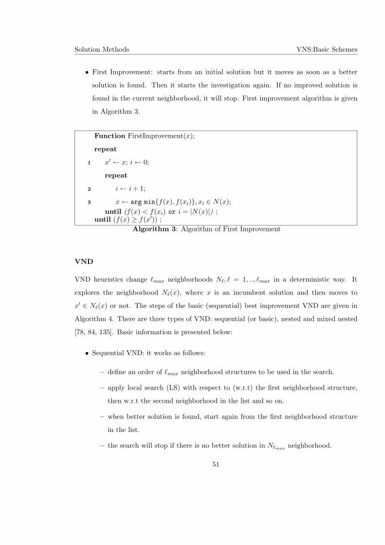
Solution Methods VNS:Basic Schemes
• First Improvement: starts from an initial solution but it moves as soon as a better
solution is found. Then it starts the investigation again. If no improved solution is
found in the current neighborhood, it will stop. First improvement algorithm is given
in Algorithm 3.
Function FirstImprovement(x);
repeat
x′ ← x; i ← 0;1
repeat
i ← i + 1;2
x ← arg min{f(x), f(xi)}, xi ∈ N(x);3
until (f(x) < f(xi) or i = |N(x)|) ;until (f(x) ≥ f(x′)) ;
Algorithm 3: Algorithm of First Improvement
VND
VND heuristics change `max neighborhoods N`, ` = 1, .., `max in a deterministic way. It
explores the neighborhood N`(x), where x is an incumbent solution and then moves to
x′ ∈ N`(x) or not. The steps of the basic (sequential) best improvement VND are given in
Algorithm 4. There are three types of VND: sequential (or basic), nested and mixed nested
[78, 84, 135]. Basic information is presented below:
• Sequential VND: it works as follows:
– define an order of `max neighborhood structures to be used in the search.
– apply local search (LS) with respect to (w.r.t) the first neighborhood structure,
then w.r.t the second neighborhood in the list and so on.
– when better solution is found, start again from the first neighborhood structure
in the list.
– the search will stop if there is no better solution in N`max neighborhood.
51
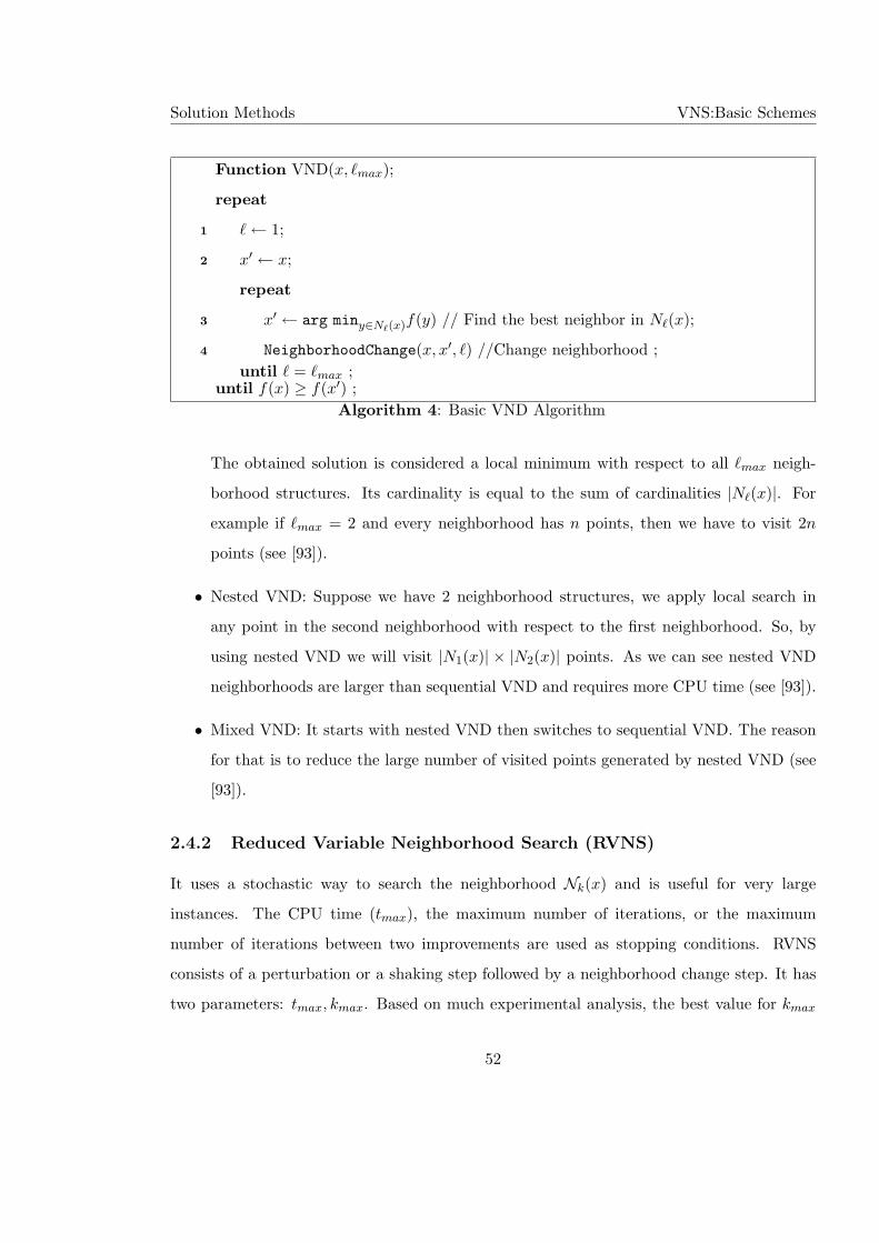
Solution Methods VNS:Basic Schemes
Function VND(x, `max);
repeat
` ← 1;1
x′ ← x;2
repeat
x′ ← arg miny∈N`(x)f(y) // Find the best neighbor in N`(x);3
NeighborhoodChange(x, x′, `) //Change neighborhood ;4
until ` = `max ;until f(x) ≥ f(x′) ;
Algorithm 4: Basic VND Algorithm
The obtained solution is considered a local minimum with respect to all `max neigh-
borhood structures. Its cardinality is equal to the sum of cardinalities |N`(x)|. For
example if `max = 2 and every neighborhood has n points, then we have to visit 2n
points (see [93]).
• Nested VND: Suppose we have 2 neighborhood structures, we apply local search in
any point in the second neighborhood with respect to the first neighborhood. So, by
using nested VND we will visit |N1(x)| × |N2(x)| points. As we can see nested VND
neighborhoods are larger than sequential VND and requires more CPU time (see [93]).
• Mixed VND: It starts with nested VND then switches to sequential VND. The reason
for that is to reduce the large number of visited points generated by nested VND (see
[93]).
2.4.2 Reduced Variable Neighborhood Search (RVNS)
It uses a stochastic way to search the neighborhood Nk(x) and is useful for very large
instances. The CPU time (tmax), the maximum number of iterations, or the maximum
number of iterations between two improvements are used as stopping conditions. RVNS
consists of a perturbation or a shaking step followed by a neighborhood change step. It has
two parameters: tmax, kmax. Based on much experimental analysis, the best value for kmax
52
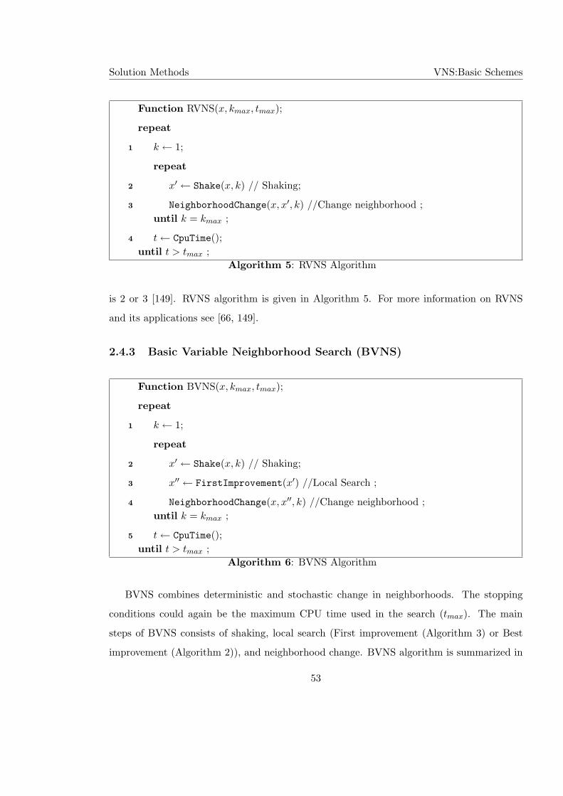
Solution Methods VNS:Basic Schemes
Function RVNS(x, kmax, tmax);
repeat
k ← 1;1
repeat
x′ ← Shake(x, k) // Shaking;2
NeighborhoodChange(x, x′, k) //Change neighborhood ;3
until k = kmax ;
t ← CpuTime();4
until t > tmax ;Algorithm 5: RVNS Algorithm
is 2 or 3 [149]. RVNS algorithm is given in Algorithm 5. For more information on RVNS
and its applications see [66, 149].
2.4.3 Basic Variable Neighborhood Search (BVNS)
Function BVNS(x, kmax, tmax);
repeat
k ← 1;1
repeat
x′ ← Shake(x, k) // Shaking;2
x′′ ← FirstImprovement(x′) //Local Search ;3
NeighborhoodChange(x, x′′, k) //Change neighborhood ;4
until k = kmax ;
t ← CpuTime();5
until t > tmax ;Algorithm 6: BVNS Algorithm
BVNS combines deterministic and stochastic change in neighborhoods. The stopping
conditions could again be the maximum CPU time used in the search (tmax). The main
steps of BVNS consists of shaking, local search (First improvement (Algorithm 3) or Best
improvement (Algorithm 2)), and neighborhood change. BVNS algorithm is summarized in
53
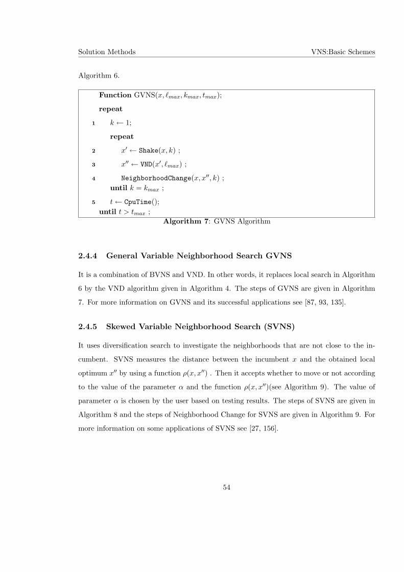
Solution Methods VNS:Basic Schemes
Algorithm 6.
Function GVNS(x, `max, kmax, tmax);
repeat
k ← 1;1
repeat
x′ ← Shake(x, k) ;2
x′′ ← VND(x′, `max) ;3
NeighborhoodChange(x, x′′, k) ;4
until k = kmax ;
t ← CpuTime();5
until t > tmax ;Algorithm 7: GVNS Algorithm
2.4.4 General Variable Neighborhood Search GVNS
It is a combination of BVNS and VND. In other words, it replaces local search in Algorithm
6 by the VND algorithm given in Algorithm 4. The steps of GVNS are given in Algorithm
7. For more information on GVNS and its successful applications see [87, 93, 135].
2.4.5 Skewed Variable Neighborhood Search (SVNS)
It uses diversification search to investigate the neighborhoods that are not close to the in-
cumbent. SVNS measures the distance between the incumbent x and the obtained local
optimum x′′ by using a function ρ(x, x′′) . Then it accepts whether to move or not according
to the value of the parameter α and the function ρ(x, x′′)(see Algorithm 9). The value of
parameter α is chosen by the user based on testing results. The steps of SVNS are given in
Algorithm 8 and the steps of Neighborhood Change for SVNS are given in Algorithm 9. For
more information on some applications of SVNS see [27, 156].
54
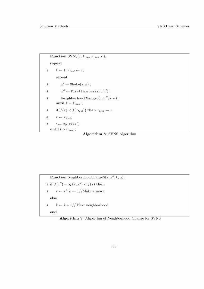
Solution Methods VNS:Basic Schemes
Function SVNS(x, kmax, tmax, α);
repeat
k ← 1, xbest ← x;1
repeat
x′ ← Shake(x, k) ;2
x′′ ← FirstImprovement(x′) ;3
NeighborhoodChangeS(x, x′′, k, α) ;4
until k = kmax ;
if(f(x) < f(xbest)) then xbest ← x;5
x ← xbest;6
t ← CpuTime();7
until t > tmax ;Algorithm 8: SVNS Algorithm
Function NeighborhoodChangeS(x, x′′, k, α);
if f(x′′)− αρ(x, x′′) < f(x) then1
x ← x′′; k ← 1//Make a move;2
else
k ← k + 1// Next neighborhood;3
end
Algorithm 9: Algorithm of Neighborhood Change for SVNS
55
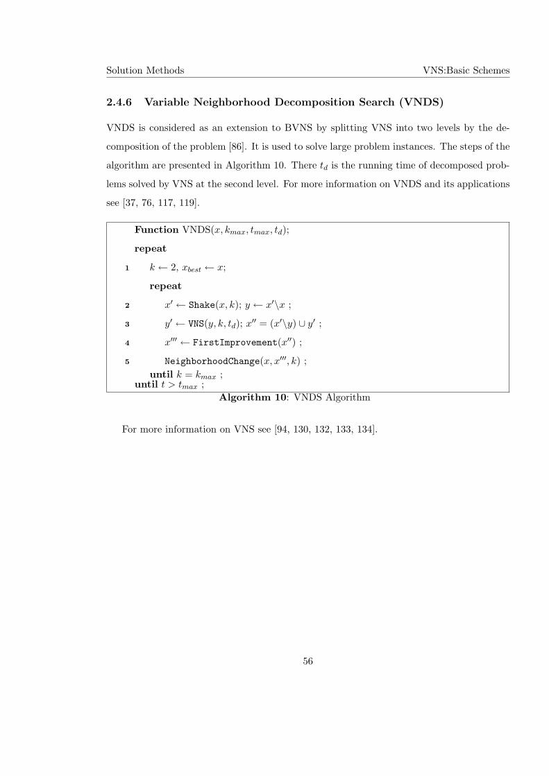
Solution Methods VNS:Basic Schemes
2.4.6 Variable Neighborhood Decomposition Search (VNDS)
VNDS is considered as an extension to BVNS by splitting VNS into two levels by the de-
composition of the problem [86]. It is used to solve large problem instances. The steps of the
algorithm are presented in Algorithm 10. There td is the running time of decomposed prob-
lems solved by VNS at the second level. For more information on VNDS and its applications
see [37, 76, 117, 119].
Function VNDS(x, kmax, tmax, td);
repeat
k ← 2, xbest ← x;1
repeat
x′ ← Shake(x, k); y ← x′\x ;2
y′ ← VNS(y, k, td); x′′ = (x′\y) ∪ y′ ;3
x′′′ ← FirstImprovement(x′′) ;4
NeighborhoodChange(x, x′′′, k) ;5
until k = kmax ;until t > tmax ;
Algorithm 10: VNDS Algorithm
For more information on VNS see [94, 130, 132, 133, 134].
56
Chapter 3
General Formulation for ADVRP
As we mentioned before the Distance–Constrained Vehicle Routing Problem (DVRP) is
defined as follows: find the optimal set of tours to connect the depot to n customers with m
vehicles, such that:
• every customer is served exactly once.
• every vehicle starts and ends its tour at the depot.
• the total distance travelled by each vehicle in the solution is less than or equal to the
maximum distance allowed (Dmax).
In this chapter we present a general flow-based formulation (see [9]) that proved to be an
effective and efficient formulae with confirmation by computational results. This formulation
is compared with the adapted one. It appears that our formulation solves ADVRP faster
and is able to improve the quality of the objective function. In other words, it is able to
find the optimal solution whereas the adapted formulation could only find the best feasi-
ble solution without guarantee of optimality because of time. Comparisons between these
two formulations are performed on random test instances with dimensions from 40 to 200
customers.
In addition, we present Kara formulation which is similar to our formulation, but the
difference is that Kara formulation requires the assumption of the triangle inequality.
57
General Formulation for ADVRP Introduction
The structure of this chapter is as follows: the introduction in Section 3.1 contains
the common parts in formulations. Section 3.2 presents the adapted bus school routing
formulation. Section 3.3 presents Kara formulation which deals with matrices that satisfy
the triangle inequality and section 3.4 presents our general formulation with an illustrative
example. The computational results are in section 3.5. Finally, section 3.6 is a conclusion.
3.1 Introduction
Let N = {1, 2..., n − 1} denotes the set of customers and V = N ∪ {0} denotes the set of
vertices where (0) is an index for the depot. The set of arcs is denoted as A = {(i, j) ∈V ×V, i 6= j}. The travelled distance from vertex i to vertex j is denoted by cij . The number
of vehicles is denoted by m. The decision binary variables xij are defined as follows:
xij =
1 if the arc (i, j) belongs to an optimal tour;
0 otherwise.(3.1)
The continuous variables (zij) represent the total length travelled from the depot to
vertex j, where i is the predecessor of vertex j. The common part of the general formulation
and the adapted formulation of ADVRP is given below:
f(S) = min∑
(i,j)∈A
cijxij (3.2)
where xij satisfies these conditions
∑
i∈V
xij = 1 ∀ j ∈ N (3.3)
∑
j∈V
xij = 1 ∀ i ∈ N (3.4)
∑
i∈N
xi0 = m (3.5)
∑
j∈N
x0j = m (3.6)
58
General Formulation for ADVRP Adapted Formulation
∑
(i,j)∈A
zij −∑
(i,j)∈A
zji −∑
j∈V
cijxij = 0 ∀ i ∈ N (3.7)
xij ∈ {0, 1} ∀ (i, j) ∈ A. (3.8)
Obviously, there are 2-index variables and a polynomial number of constraints. This
model is known as flow (arc) based model since constraint (3.7) is a typical flow constraint.
It says that the distance from vertex i to any other vertex j on the tour should be equal
to the difference between the distance from the depot to vertex i and the distance from the
depot to vertex j. The constraints (3.3, 3.4) ensure that the indegrees and outdegrees of
each vertex equal to 1. Constraints (3.5, 3.6) express that indegrees and outdegrees of the
depot equal to the number of vehicles (m).
3.2 Adapted Formulation
The adapted formulation was originally the Bus school routing problem (BSRP) described
as the collection of students from (n) bus stops to be brought to school (or collection from
the school to be brought to bus stops), and the number of buses is given (m). For more
information on BSRP see [20].
The objective function is to minimize the total distance (cost or time), provided:
• the travelled distance for each bus has to be less than or equal to the given value
(Dmax).
• each bus stop can only be used by one bus.
• each bus stop can only be in one tour.
• every tour must have one stop at least.
• the number of students in each tour must not exceed the capacity of the bus.
Kara [101] noticed that the special case of BSRP is DVRP. In fact, if we ignore the ca-
pacity constraints and consider the number of buses constant, then the following constraints
need to be added to get an Adapted BSRP formulation:
59
General Formulation for ADVRP Kara Formulation
zij ≤ Dmaxxij ∀ (i, j) ∈ A (3.9)
zij ≥ cijxij i 6= 0, ∀(i, j) ∈ A (3.10)
z0i = c0ix0i ∀ i ∈ N (3.11)
Constraints (3.3) - (3.10) for morning routes (collection), and constraints (3.3) - (3.11) for
afternoon routes (delivery) are used in [42]. We do not need both if we consider the origin
of the bus and its destination (school) as a single vertex (depot). Therefore, we will use
constraints(3.3) - (3.11) to find the solution to ADVRP. We are allowed to consider the
depot and the school as the same vertex since the distance matrix is asymmetric. This
formulation is compared with our general formulation.
3.3 Kara Formulation
Now we discuss another formulation which is similar to ours, that is Kara’s flow based
formulation [98]. Kara’s formulation is given as follows:
f(S) = min∑
(i,j)∈A
dijxij (3.12)
where xij satisfies these conditions
∑
i∈V
xij = 1 ∀ j ∈ N (3.13)
∑
j∈V
xij = 1 ∀ i ∈ N (3.14)
∑
i∈N
xi0 = m (3.15)
∑
i∈N
x0i = m (3.16)
∑
(i,j)∈A
zij −∑
(i,j)∈A
zji −∑
j∈V
dijxij = 0 ∀ i ∈ N (3.17)
zij ≤ (Dmax − dj0)xij j 6= 0,∀(i, j) ∈ A (3.18)
60
General Formulation for ADVRP General Formulation for ADVRP
zi0 ≤ Dmaxxi0 j ∈ N (3.19)
zij ≥ (dij + d0i)xij i 6= 0, ∀(i, j) ∈ A (3.20)
z0i = d0ix0i ∀ i ∈ N (3.21)
xij ∈ {0, 1} ∀ (i, j) ∈ A. (3.22)
The dij in this formulation represents the shortest distance between vertex i and vertex j.
This means that the distance matrix in Kara’s formulation is required to satisfy a triangle
inequality, while our general formulation does not need this requirement. Therefore, these
two formulations differ only on the assumption of the triangle inequality.
In [98], Kara compares his formulation with Waters formulation (see [165]), where Kara
formulation outperformed Waters formulation.
3.4 General Formulation for ADVRP
In this formulation, we use the concept of shortest distance to and from the depot. The
same objective function and the same constraints (3.3) - (3.8), (3.11) are used. In addition,
we add the following constraints:
zij ≤ (Dmax − dj0)xij j 6= 0,∀(i, j) ∈ A (3.23)
zij ≥ (cij + d0i)xij i 6= 0, ∀(i, j) ∈ A (3.24)
zi0 ≤ (Dmax)xi0 ∀ i ∈ N (3.25)
Here d0i represents the shortest distance from the depot to vertex i and dj0 represents
the shortest distance from vertex j to the depot. cij represents the travelled distance from
vertex i to vertex j. Values of d0i and dj0 have been found and added as the last two rows
of the distance matrices.
61
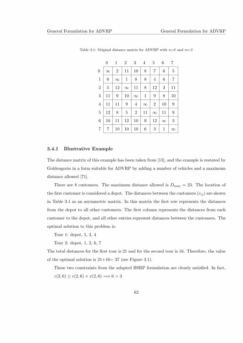
General Formulation for ADVRP General Formulation for ADVRP
Table 3.1: Original distance matrix for ADVRP with n=8 and m=2
0 1 2 3 4 5 6 7
0 ∞ 2 11 10 8 7 6 5
1 6 ∞ 1 8 8 4 6 7
2 5 12 ∞ 11 8 12 3 11
3 11 9 10 ∞ 1 9 8 10
4 11 11 9 4 ∞ 2 10 9
5 12 8 5 2 11 ∞ 11 9
6 10 11 12 10 9 12 ∞ 3
7 7 10 10 10 6 3 1 ∞
3.4.1 Illustrative Example
The distance matrix of this example has been taken from [13], and the example is restated by
Goldengorin in a form suitable for ADVRP by adding a number of vehicles and a maximum
distance allowed [71].
There are 8 customers. The maximum distance allowed is Dmax = 23. The location of
the first customer is considered a depot. The distances between the customers (cij) are shown
in Table 3.1 as an asymmetric matrix. In this matrix the first row represents the distances
from the depot to all other customers. The first column represents the distances from each
customer to the depot, and all other entries represent distances between the customers. The
optimal solution to this problem is:
Tour 1: depot, 5, 3, 4
Tour 2: depot, 1, 2, 6, 7
The total distances for the first tour is 21 and for the second tour is 16. Therefore, the value
of the optimal solution is 21+16= 37 (see Figure 3.1).
These two constraints from the adapted BSRP formulation are clearly satisfied. In fact,
z(2, 6) ≥ c(2, 6)× x(2, 6) =⇒ 6 > 3
62

General Formulation for ADVRP Computational Results
Figure 3.1: Optimal solution (n=8, m=2, Dmax =23)
z(3, 4) ≥ c(3, 4)× x(3, 4) =⇒ 10 > 1
With our formulation the values of d(0,2) and d(0,3) are 3 and 8 respectively. Therefore,
we have:
z(2, 6) ≥ (d(0, 2) + c(2, 6))x(2, 6) =⇒ 6 ≥ (3 + 3)× 1
z(3, 4) ≥ (d(0, 3) + c(3, 4))x(3, 4) =⇒ 10 ≥ (8 + 1)× 1
It is clear that our formulation is tighter than the adapted BSRP.
3.5 Computational Results
Computers. All experiments were implemented under windows XP and on intel (R)
Core(TM)2 CPU [email protected], with 3.24 GB of RAM. The code is written in C++ lan-
guage, and the solver is CPLEX 11.
Test Instances. A random number generator has been used to generate a full asymmetric
distance matrix as in [7]. The size of the distance matrix (n) is chosen to be {40, 60, 80,
100} for small test instances or{120, 140, 160, 180, 200} for large test instances. For each n,
two different number of vehicles were defined as follows:
63
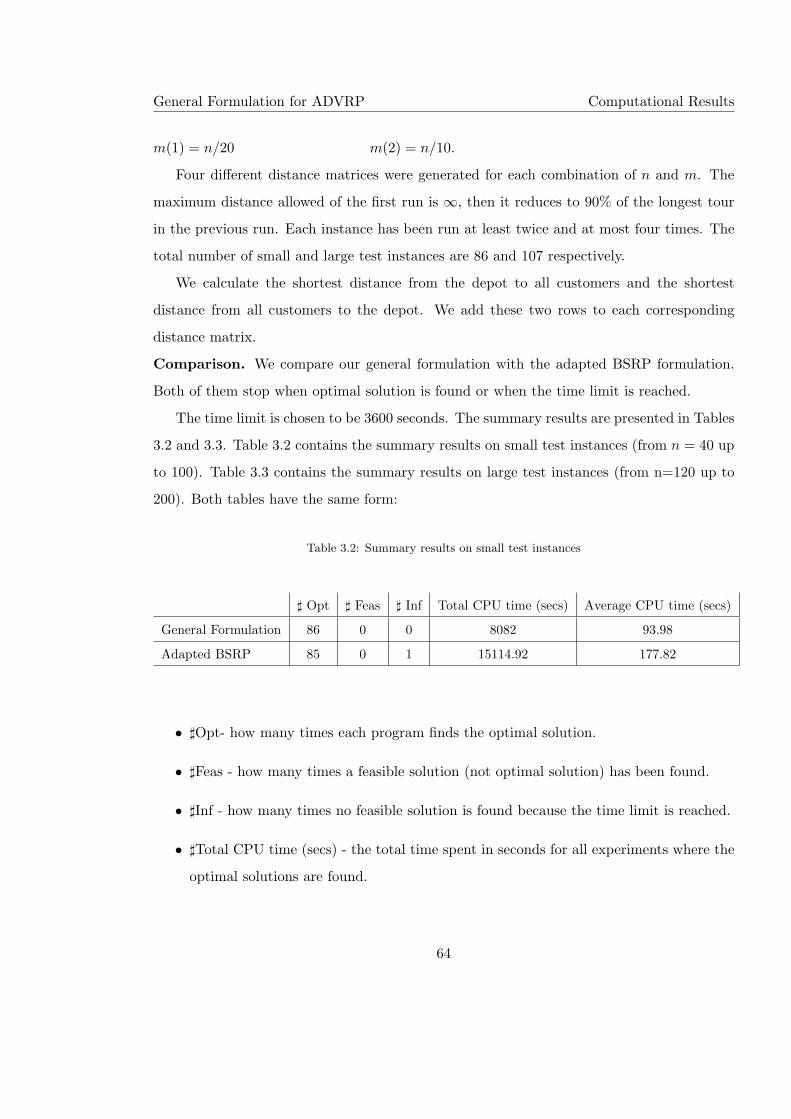
General Formulation for ADVRP Computational Results
m(1) = n/20 m(2) = n/10.
Four different distance matrices were generated for each combination of n and m. The
maximum distance allowed of the first run is ∞, then it reduces to 90% of the longest tour
in the previous run. Each instance has been run at least twice and at most four times. The
total number of small and large test instances are 86 and 107 respectively.
We calculate the shortest distance from the depot to all customers and the shortest
distance from all customers to the depot. We add these two rows to each corresponding
distance matrix.
Comparison. We compare our general formulation with the adapted BSRP formulation.
Both of them stop when optimal solution is found or when the time limit is reached.
The time limit is chosen to be 3600 seconds. The summary results are presented in Tables
3.2 and 3.3. Table 3.2 contains the summary results on small test instances (from n = 40 up
to 100). Table 3.3 contains the summary results on large test instances (from n=120 up to
200). Both tables have the same form:
Table 3.2: Summary results on small test instances
] Opt ] Feas ] Inf Total CPU time (secs) Average CPU time (secs)
General Formulation 86 0 0 8082 93.98
Adapted BSRP 85 0 1 15114.92 177.82
• ]Opt- how many times each program finds the optimal solution.
• ]Feas - how many times a feasible solution (not optimal solution) has been found.
• ]Inf - how many times no feasible solution is found because the time limit is reached.
• ]Total CPU time (secs) - the total time spent in seconds for all experiments where the
optimal solutions are found.
64
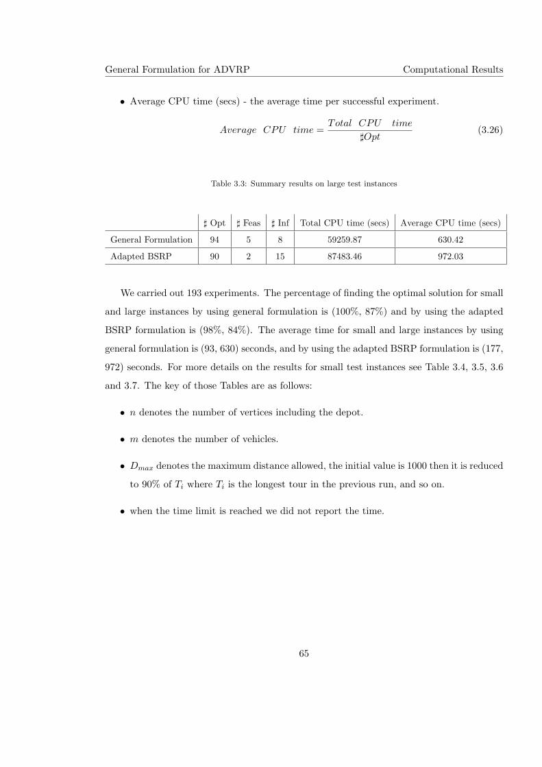
General Formulation for ADVRP Computational Results
• Average CPU time (secs) - the average time per successful experiment.
Average CPU time =Total CPU time
]Opt(3.26)
Table 3.3: Summary results on large test instances
] Opt ] Feas ] Inf Total CPU time (secs) Average CPU time (secs)
General Formulation 94 5 8 59259.87 630.42
Adapted BSRP 90 2 15 87483.46 972.03
We carried out 193 experiments. The percentage of finding the optimal solution for small
and large instances by using general formulation is (100%, 87%) and by using the adapted
BSRP formulation is (98%, 84%). The average time for small and large instances by using
general formulation is (93, 630) seconds, and by using the adapted BSRP formulation is (177,
972) seconds. For more details on the results for small test instances see Table 3.4, 3.5, 3.6
and 3.7. The key of those Tables are as follows:
• n denotes the number of vertices including the depot.
• m denotes the number of vehicles.
• Dmax denotes the maximum distance allowed, the initial value is 1000 then it is reduced
to 90% of Ti where Ti is the longest tour in the previous run, and so on.
• when the time limit is reached we did not report the time.
65
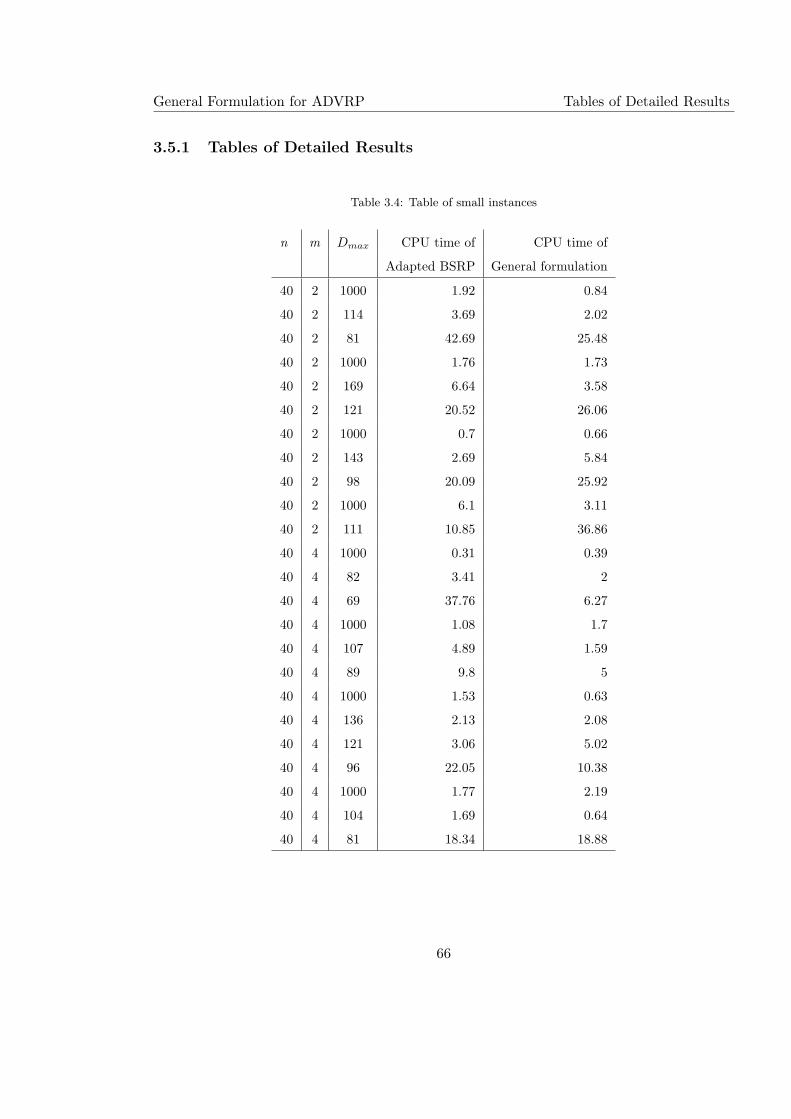
General Formulation for ADVRP Tables of Detailed Results
3.5.1 Tables of Detailed Results
Table 3.4: Table of small instances
n m Dmax CPU time of CPU time of
Adapted BSRP General formulation
40 2 1000 1.92 0.84
40 2 114 3.69 2.02
40 2 81 42.69 25.48
40 2 1000 1.76 1.73
40 2 169 6.64 3.58
40 2 121 20.52 26.06
40 2 1000 0.7 0.66
40 2 143 2.69 5.84
40 2 98 20.09 25.92
40 2 1000 6.1 3.11
40 2 111 10.85 36.86
40 4 1000 0.31 0.39
40 4 82 3.41 2
40 4 69 37.76 6.27
40 4 1000 1.08 1.7
40 4 107 4.89 1.59
40 4 89 9.8 5
40 4 1000 1.53 0.63
40 4 136 2.13 2.08
40 4 121 3.06 5.02
40 4 96 22.05 10.38
40 4 1000 1.77 2.19
40 4 104 1.69 0.64
40 4 81 18.34 18.88
66
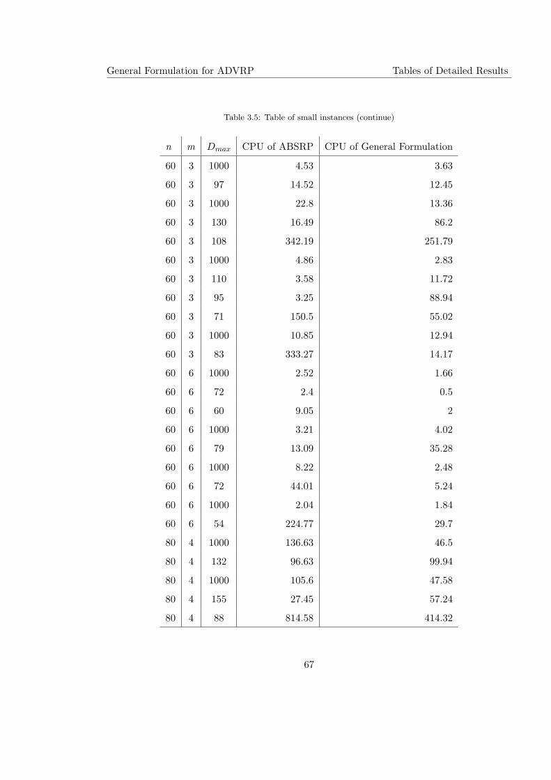
General Formulation for ADVRP Tables of Detailed Results
Table 3.5: Table of small instances (continue)
n m Dmax CPU of ABSRP CPU of General Formulation
60 3 1000 4.53 3.63
60 3 97 14.52 12.45
60 3 1000 22.8 13.36
60 3 130 16.49 86.2
60 3 108 342.19 251.79
60 3 1000 4.86 2.83
60 3 110 3.58 11.72
60 3 95 3.25 88.94
60 3 71 150.5 55.02
60 3 1000 10.85 12.94
60 3 83 333.27 14.17
60 6 1000 2.52 1.66
60 6 72 2.4 0.5
60 6 60 9.05 2
60 6 1000 3.21 4.02
60 6 79 13.09 35.28
60 6 1000 8.22 2.48
60 6 72 44.01 5.24
60 6 1000 2.04 1.84
60 6 54 224.77 29.7
80 4 1000 136.63 46.5
80 4 132 96.63 99.94
80 4 1000 105.6 47.58
80 4 155 27.45 57.24
80 4 88 814.58 414.32
67
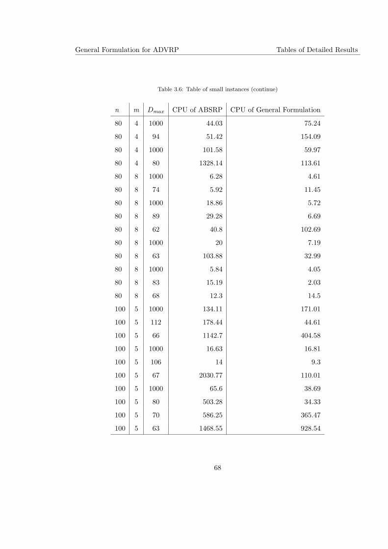
General Formulation for ADVRP Tables of Detailed Results
Table 3.6: Table of small instances (continue)
n m Dmax CPU of ABSRP CPU of General Formulation
80 4 1000 44.03 75.24
80 4 94 51.42 154.09
80 4 1000 101.58 59.97
80 4 80 1328.14 113.61
80 8 1000 6.28 4.61
80 8 74 5.92 11.45
80 8 1000 18.86 5.72
80 8 89 29.28 6.69
80 8 62 40.8 102.69
80 8 1000 20 7.19
80 8 63 103.88 32.99
80 8 1000 5.84 4.05
80 8 83 15.19 2.03
80 8 68 12.3 14.5
100 5 1000 134.11 171.01
100 5 112 178.44 44.61
100 5 66 1142.7 404.58
100 5 1000 16.63 16.81
100 5 106 14 9.3
100 5 67 2030.77 110.01
100 5 1000 65.6 38.69
100 5 80 503.28 34.33
100 5 70 586.25 365.47
100 5 63 1468.55 928.54
68
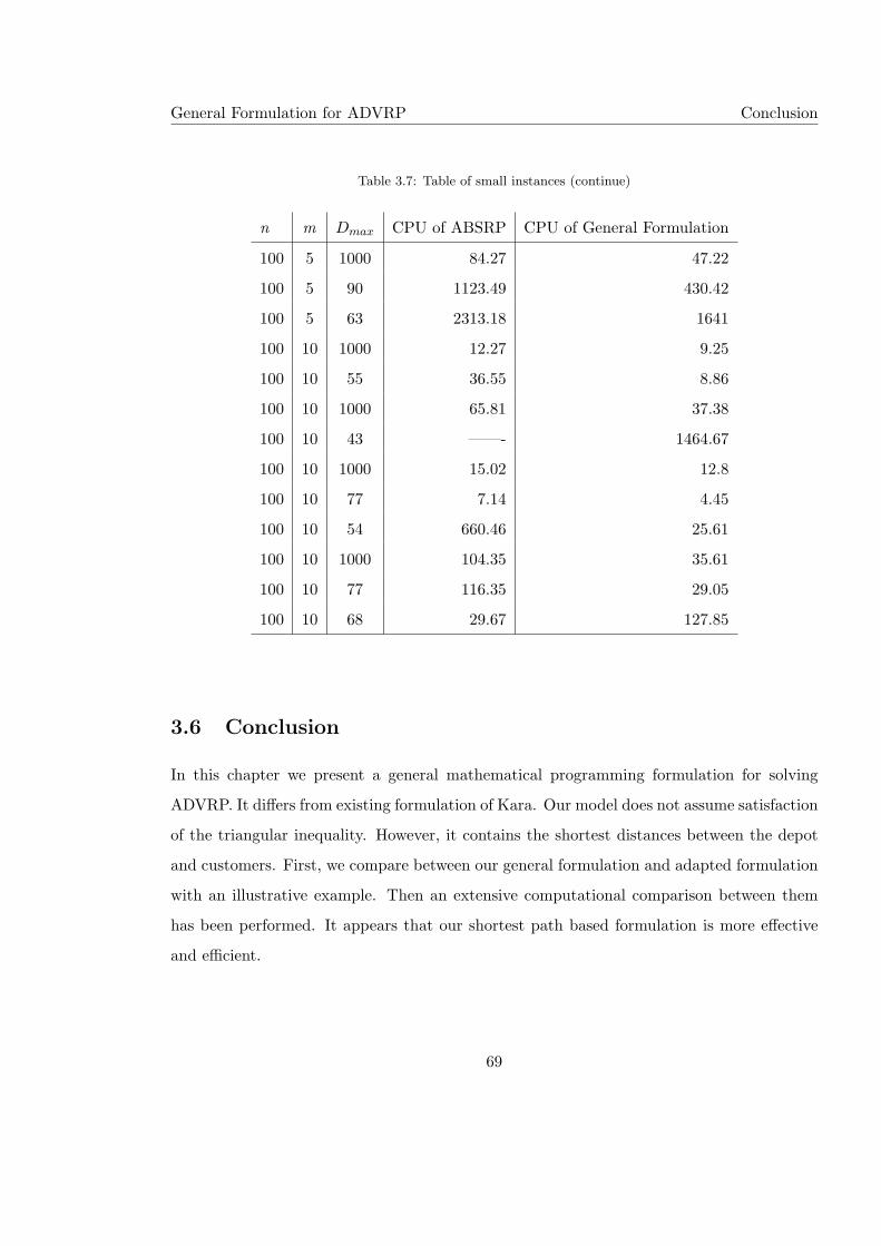
General Formulation for ADVRP Conclusion
Table 3.7: Table of small instances (continue)
n m Dmax CPU of ABSRP CPU of General Formulation
100 5 1000 84.27 47.22
100 5 90 1123.49 430.42
100 5 63 2313.18 1641
100 10 1000 12.27 9.25
100 10 55 36.55 8.86
100 10 1000 65.81 37.38
100 10 43 ——- 1464.67
100 10 1000 15.02 12.8
100 10 77 7.14 4.45
100 10 54 660.46 25.61
100 10 1000 104.35 35.61
100 10 77 116.35 29.05
100 10 68 29.67 127.85
3.6 Conclusion
In this chapter we present a general mathematical programming formulation for solving
ADVRP. It differs from existing formulation of Kara. Our model does not assume satisfaction
of the triangular inequality. However, it contains the shortest distances between the depot
and customers. First, we compare between our general formulation and adapted formulation
with an illustrative example. Then an extensive computational comparison between them
has been performed. It appears that our shortest path based formulation is more effective
and efficient.
69
Chapter 4
Multistart Branch and Bound for
ADVRP
In this chapter we revise and modify a branch-and-bound method for solving the asymmetric
distance–constrained vehicle routing problem (ADVRP) which is based on an old branch and
bound method suggested by Laporte et al. in 1987 [113].
As mentioned before, this method is based on reformulating the distance–constrained
vehicle routing problem into a travelling salesman problem and using assignment problem as
a lower bounding procedure. In addition, the algorithm uses the best first strategy and new
tolerance based branching rules. This method was fast but memory consuming. To overcome
the memory problem, we introduce randomness, in case of ties, in choosing the node of the
search tree. If an optimal solution is not found, we restart our procedure. This restart due
to lack of memory so cannot continue with the current tree. In this way, we get a multistart
branch and bound method.
As far as we know, the instances solved exactly (up to 1000 customers) are much larger
than instances considered for other VRP models from recent literature. So, despite of its
simplicity, this proposed algorithm is capable of solving the largest instances ever solved in
literature. Moreover, this approach is general and may be used to solve other types of vehicle
routing problems. This chapter is based on our article presented in [8]. The extended version
70
Multistart Branch and Bound for ADVRP Introduction
has been published in this book [10] and in [11].
The structure of this chapter is as follows. In section 4.1, we present the introduction.
Section 4.2 presents mathematical programming formulations of ADVRP. In section 4.3 we
discuss the deterministic and stochastic Branch and Bound method for ADVRP. In section
4.4 we present our multistart approach for solving ADVRP. Section 4.5 contains details
regarding data structure that we used in our implementation. Computational results are
provided in section 4.6. Finally in section 4.7 we give a conclusion and future research
directions.
4.1 Introduction
A variety of integer programming formulations have been proposed for VRPs, including the
so-called two-index and three-index formulations, the set partitioning formulation, and vari-
ous formulations based on extra variables representing the flow of one or more commodities
(see e.g. survey and formulation comparisons in [121]). In addition, recent solution tech-
niques are mostly based on branch-and-cut or on branch-and-cut-and-price (see [17, 142] and
recent survey in [16]).
In this chapter we suggest a new simple algorithm for solving ADVRP that is based
on Branch and Bound (B&B) method. As in [113], the ADVRP is first transformed to
the travelling salesman problem (TSP). The lower bounds are obtained by relaxing the
subtour elimination and maximum distance constraints. Thus the Assignment problem (AP)
is solved in each node of the B&B tree. In addition, the best-first-search strategy and adapted
tolerance based rules for branching are used as in [7]. That is, the next node in the tree is
the one with the smallest relaxed objective function value. In the case of a tie, we use two
tie-breaking rules: (i) the last one in the list (TOL-ADVRP) [7]; (ii) the random one among
them (RND-ADVRP).
We found that stochastic B&B based method (RND-ADVRP) is faster than the determin-
istic B&B based method (TOL-ADVRP) but it is still memory consuming. That is why we
suggested multistart B&B method (MSBB-ADVRP). It simply uses random tie-breaking rule
71
Multistart Branch and Bound for ADVRP Mathematical Programming Formulations
in the selection of the next subproblem and restart again. Computational results show that
we are able to provide exact solutions for instances with up to 1000 customers. The size of
problems could be even larger if a more powerful computer (with larger memory) is used.
As far as we know these instances are much larger than any other instances considered for
similar VRP models and exact solution approaches from the recent literature. For example,
in the recent paper by Baldacci and Mingozzi [15], several VRP problem types are studied
and sophisticated exact solution methods tested. The largest instances solved had 199 cus-
tomers. Therefore, our simple algorithms are capable of solving the largest instances ever
solved in the literature.
4.2 Mathematical Programming Formulations for ADVRP
In this section we give two mathematical programming formulations of ADVRP. The first
one, so-called flow based formulation, is used for comparison purposes in the computational
results section. The second is based on transformation of ADVRP to asymmetric travelling
salesman problem (TSP). We use its relaxation in our B&B exact method, that will be
described in section (4.3).
Let N ′ = {1, 2..., n−1} denotes the set of customers and V ′ = N ′∪{0} denotes the set of
vertices where 0 is the index of the depot. A set of arcs is denoted by A′ where A′ is defined
as follows: A′ = {(i, j) ∈ V ′ × V ′ : i 6= j}. The distance matrix is denoted by D′ = [d′ij ]
where d′ij presents the travelled distance from vertex i to vertex j, the number of vehicles is
denoted by m. The maximum distance allowed is denoted by Dmax. The shortest distance
between vertex i and vertex j is denoted by cij .
The decision binary variable xij is defined as follows:
xij =
1 if the arc (i, j) belongs to any tour and i 6= j;
0 otherwise.(4.1)
72
Multistart Branch and Bound for ADVRP Mathematical Programming Formulations
4.2.1 Flow Based Formulation
For the sake of comparison, we use flow based formulation of ADVRP with a polynomial
number of variables and constraints, without copying depots. This is achieved by introducing
the new set of variables zij . They present the shortest length travelled from the depot to
vertex j, where vertex i is the predecessor of vertex j. The formulation of ADVRP, that will
be later used with CPLEX solver (CPLEX-ADVRP), is given below [98]:
f(S) = min∑
(i,j)∈A′cijxij (4.2)
subject to
∑
i∈V ′xij = 1 ∀ j ∈ N ′ (4.3)
∑
j∈V ′xij = 1 ∀ i ∈ N ′ (4.4)
∑
i∈N ′xi0 = m (4.5)
∑
j∈N ′x0j = m (4.6)
∑
(i,j)∈A′zij −
∑
(j,i)∈A′zji −
∑
j∈V ′cijxij = 0 ∀ i ∈ N ′ (4.7)
zij ≤ (Dmax − cj0)xij ∀ j 6= 0, ∀(i, j) ∈ A′ (4.8)
zi0 ≤ Dmaxxi0 ∀i ∈ N ′ (4.9)
zij ≥ (cij + c0i)xij ∀ i 6= 0, ∀(i, j) ∈ A′ (4.10)
z0i = c0ix0i ∀ i ∈ N ′ (4.11)
xij ∈ {0, 1} ∀ (i, j) ∈ A′. (4.12)
Obviously, there are a polynomial number of variables and constraints. This model is known
as flow based model since constraint (4.7) is a typical flow constraint. It says that the
73
Multistart Branch and Bound for ADVRP Mathematical Programming Formulations
distance from vertex i to any other vertex j on the tour should be equal to the difference
between the distance from the depot to vertex i and the distance from the depot to vertex j.
Constraint (4.8) indicates that the total distance from the depot to vertex j and the shortest
distance from vertex j to the depot directly are less than or equal to the maximum distance
allowed. The constraint (4.9) checks that the total distance travelled up to the depot is less
than or equal to the maximum distance allowed. In addition, according to constraint (4.10)
the total distance from the depot to vertex j should be greater than or equal to the distance
from the depot to vertex i plus the distance from vertex i to vertex j. Constraint (4.11)
gives the initial value for z0i, which is equal to the distance from the depot to vertex i. Last
constraint (4.12) introduces the decision variables xij as binary variables.
4.2.2 TSP Formulation
The TSP formulation may be obtained by adding m−1 copies of the depot to V ′ [120]. Now
there are n + m− 1 vertices in the new augmented directed graph G(V, A), where
V = V′ ∪ {n, n + 1, . . . , n + m− 2}.
The distance matrix D is obtained from D′ by the following transformation rules where
i, j ∈ V :
dij =
d′ij if (0 ≤ i < n, 0 ≤ j < n, i 6= j)
d′0j if (i ≥ n, 0 < j < n)
d′i0 if (0 < i < n, j ≥ n)
∞ otherwise
Then the formulation of TSP [39] is given below (4.13 - 4.16) as follows:
f(S) = min∑
(i,j)∈A
dijxij (4.13)
where xij satisfies these conditions
∑
i
xij = 1 ∀ j ∈ V (4.14)
74
Multistart Branch and Bound for ADVRP Branch and Bound
∑
j
xij = 1 ∀ i ∈ V (4.15)
∑
i,j∈U
xij ≤| U | −1 ∀ U ⊂ V \{0}, |U | ≥ 2, (4.16)
+ distance constraints (4.17)
The constraints (4.14) and (4.15) ensure that indegree and outdegree of each vertex
are equal to 1. The constraint (4.16) eliminates subtours, where U is a subset of V \{0}containing at least 2 vertices. To formulate ADVRP, in addition to (4.13)-(4.16), we need
to add the distance constraint (4.17), which checks if the total distance for each tour is less
than the maximum distance allowed (Dmax).
The downside of this formulation is the exponential number of constraints in (4.16),
since the number of subsets U is exponential. However, in our B&B method, which will be
explained in the next section, this set of constraints will be relaxed.
DVRP may be seen as a special case of VRP with time windows constraints (VRPTW)
[121]. As mentioned in Section 1.1, VRPTW requires a time tij ≥ 0 to traverse arc (i, j),
that includes any time used to serve customer i ∈ N ′. The service must begin within the
time window [ei, li] for each customer, where 0 ≤ ei ≤ li ≤ ∞. In addition, each vehicle is
allowed to leave the depot at time e0 or after, and come back to depot by time l0 or before.
A vehicle can wait before serving any customer or after . The DVRP can be viewed as a
special case of the VRPTW by setting tij = dij , ei = d0i and li = Dmax − di0.
4.3 Single Start Branch and Bound for ADVRP (RND-ADVRP)
The branch and bound (B&B) is an exact method for solving integer programming problems.
It consists of enumerating all possible solutions within the so-called search tree and pruning
subtrees when better solutions than the current one (upper bound) cannot be found. B&B
is briefly explained below:
• The original problem is placed at the root of the branch and bound tree (or search tree).
All other nodes in the search tree represent subproblems. In solving subproblems some
75
Multistart Branch and Bound for ADVRP Branch and Bound
variables are fixed and some constraints are ignored (relaxed), so that the lower bound
is obtained.
• An initial feasible solution of good quality is usually obtained by heuristic and its
objective function value is the initial upper bound (UB). If a heuristic is not used,
then the upper bound is set to infinity (UB = ∞) and it will be updated as soon as
the feasible solution is found during the search.
• The search strategy defines the way in which we choose the next node for branching.
There are three basic branching strategies: breadth first search, depth first search and
hybrid search which is also called best first search strategy (see Section 2.1.1). In this
thesis we implement this strategy.
4.3.1 Upper Bound
The upper bound is the value of the incumbent which is the best feasible solution found so
far. Initial value of UB could be ∞ or it could be obtained by using a heuristic. Usually
heuristics provide good feasible solutions, that help to reduce the size of the search tree by
pruning any subproblem that has a value greater than UB.
In our method this value is not so useful because we use best first search which is not
affected by the value of UB. For this reason we set the value of UB to be UB = m×Dmax.
4.3.2 Lower Bounds
To apply B&B we need a lower bounding procedure that should be applied at each node
of the search tree. Of course, there are many ways to relax model (4.13)-(4.17). The more
constraints included, the better (higher) the lower bound. In fact, the set of feasible solutions
of the problem with m constraints is a subset of feasible solutions of the same problem
with m − 1 constraints. Thus, its objective function value is worse. However, adding new
constraints makes the lower bound higher.
We use AP as a lower bounding procedure of the TSP formulation given in (4.13)-
(4.15), i.e., we relax all tour elimination and maximum distance constraints (4.16) and (4.17).
76
Multistart Branch and Bound for ADVRP Branch and Bound
Although the quality of the lower bound is not high, the benefit is in using the very fast
exact Hungarian method for solving AP [104]. In this thesis we use the implementation
described in [97]. The complexity of AP at root node is O(n3) [163]. Another advantage is
that the relaxed AP solution is already an integer.
Proposition 1 Any feasible AP solution of problem (4.13)-(4.15) consists of a set of cycles,
i.e., a sequence of arcs starting and ending at the same vertex with the number of arcs in
any cycle k greater than or equal to 2 (ωk ≥ 2).
Proof. It is clear from (4.14) and (4.15) that the degree of each vertex in S is equal to 2. It
has one incoming and one out coming arc. If the matrix D was symmetric and n even, then
those cycles would contain just 2 vertices and therefore ωk = 2.
However, in all other cases, ωk is obviously larger than 2: if vertex i is assigned to vertex
j, then vertex j is not necessarily assigned to vertex i. ¥
We can present the solution of AP and TSP as a set of cycles [6]. There are 3 types of
cycles obtained by AP relaxation:
• a served cycle- contains exactly one depot.
• an unserved cycle- contains no depot.
• a path- contains more than one depot.
In the last case, each path may be divided into served cycles. Therefore, the number of
served cycles is equal to the number of depots in the path. Subsequently, the term tour is
used to denote either a served cycle, an unserved cycle or a path; the term depot is used to
denote either the original depot or a copy of the depot. A tour is called infeasible if its total
distance is larger than Dmax or if it contains no depot.
4.3.3 Branching Rules
Since the set of constraints (4.16) and (4.17) are relaxed, the AP solution may have many
infeasible tours. If the tour is infeasible, it must be destroyed, i.e., one arc should be excluded
77
Multistart Branch and Bound for ADVRP Branch and Bound
(deleted). We exclude an arc from the current infeasible solution S by giving it a large value
(∞) and then resolving AP relaxation again. Realistically, in the new solution, such an arc
will not appear, since we minimize the AP objective function. There are several ways to
remove an arc from S. We can try all possible removals (one at the time) and collect all
objective function values obtained from solving the new corresponding AP ’s.
In this thesis we use the concept of tolerance, where tolerance is one of the sensitivity
analysis techniques (for more details on sensitivity analysis see [103, 123]). The definition of
tolerance is used as a branching rule within B&B method in [161] for solving ATSP. Applying
this idea for solving ADVRP was first used in [7] and here we improve it.
The difference between the value of the objective function before and after the exclusion
of an arc in the current solution is called upper tolerance (UT) of the arc [72]. A series of arcs
have to be checked by removing one arc each time to get a new subproblem which has to be
added to the search tree. The node corresponds to the smallest objective function obtained
is chosen to branch further. Therefore, in our ADVRP tolerance based B&B (TOL-ADVRP),
the chosen subproblem corresponds to the arc which has the smallest upper tolerance. Some
preliminary results of this approach has been given in [7].
Another possibility of destroying an infeasible tour is to exclude the arc with the largest
cost [6]. B&B method uses such a branching rule called COST-ADVRP. However, based on ex-
tensive computational analysis, the results obtained with COST-ADVRP were of slightly worse
quality than those obtained by TOL-ADVRP. This is the reason why in the computational
analysis section we give TOL-ADVRP results. In TOL-ADVRP when there is more than one sub-
problem in the list of active subproblems (that have the smallest objective value) we choose
the last among them to branch next. In other words, our tie-breaking rule is deterministic.
4.3.4 Algorithm
The main steps of TOL-ADVRP algorithm are given in Algorithm 11, where we use the following
notation:
D- a distance matrix.
78
Multistart Branch and Bound for ADVRP Branch and Bound
S = {T1, T2, ..., TM(S)}- the relaxed solution obtained by AP presented as a set of tours
where M(S) is the number of tours in S.
Tk = {a1, .., at(Tk)}- the tour Tk in the solution S is presented as a set of arcs where t(Tk)
is the number of arcs in a tour k.
d(Tk)- the total travelled distance in a tour k where d(Tk) =∑
(i,j)∈Tkdij .
f(S) =∑M(s)
k=1 d(Tk) - the value of an optimal solution to AP .
S∗- an optimal solution to ADVRP.
L- the list of active subproblems (or unfathomed nodes in a search tree): it is updated
during the execution of the code.
LB- the lower bound. It is the smallest value of the objective function to AP among those
in L.
UB- the upper bound value to ADVRP, initially set to a large value.
APcnt- counts the number of nodes in B&B tree (how many times AP subroutine is called).
Maxnodes- the maximum number of nodes allowed in B&B tree. In order to prevent
termination with no memory message, we use it as a stopping condition. Here we set
Maxnodes = 100, 000.
β- the type of tie-breaking rule that has two values:
β =
0 deterministic (last in L);
1 at random.
we will use β = 0 in TOL-ADVRP algorithm. Later we will use β = 1 in RND-ADVRP
Algorithm.
ind- the variable that covers all possible outputs of the algorithm. The basic algorithm may
stop with the following outputs:
79
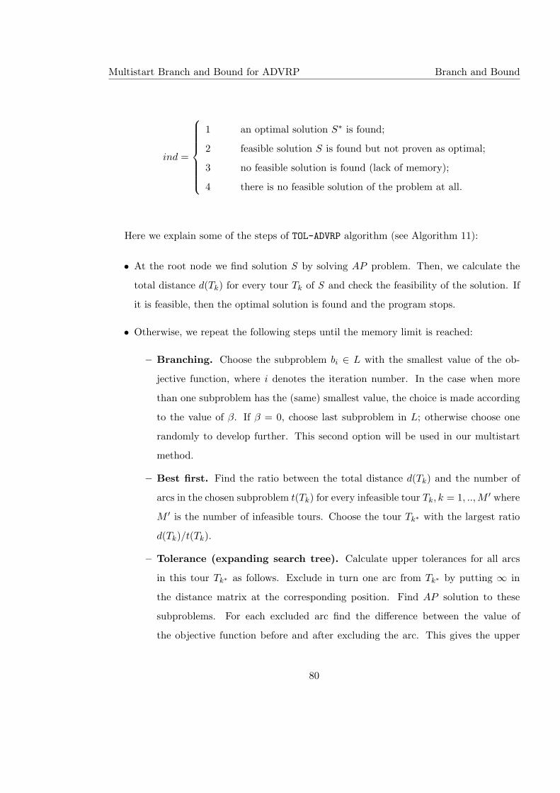
Multistart Branch and Bound for ADVRP Branch and Bound
ind =
1 an optimal solution S∗ is found;
2 feasible solution S is found but not proven as optimal;
3 no feasible solution is found (lack of memory);
4 there is no feasible solution of the problem at all.
Here we explain some of the steps of TOL-ADVRP algorithm (see Algorithm 11):
• At the root node we find solution S by solving AP problem. Then, we calculate the
total distance d(Tk) for every tour Tk of S and check the feasibility of the solution. If
it is feasible, then the optimal solution is found and the program stops.
• Otherwise, we repeat the following steps until the memory limit is reached:
– Branching. Choose the subproblem bi ∈ L with the smallest value of the ob-
jective function, where i denotes the iteration number. In the case when more
than one subproblem has the (same) smallest value, the choice is made according
to the value of β. If β = 0, choose last subproblem in L; otherwise choose one
randomly to develop further. This second option will be used in our multistart
method.
– Best first. Find the ratio between the total distance d(Tk) and the number of
arcs in the chosen subproblem t(Tk) for every infeasible tour Tk, k = 1, .., M ′ where
M ′ is the number of infeasible tours. Choose the tour Tk∗ with the largest ratio
d(Tk)/t(Tk).
– Tolerance (expanding search tree). Calculate upper tolerances for all arcs
in this tour Tk∗ as follows. Exclude in turn one arc from Tk∗ by putting ∞ in
the distance matrix at the corresponding position. Find AP solution to these
subproblems. For each excluded arc find the difference between the value of
the objective function before and after excluding the arc. This gives the upper
80
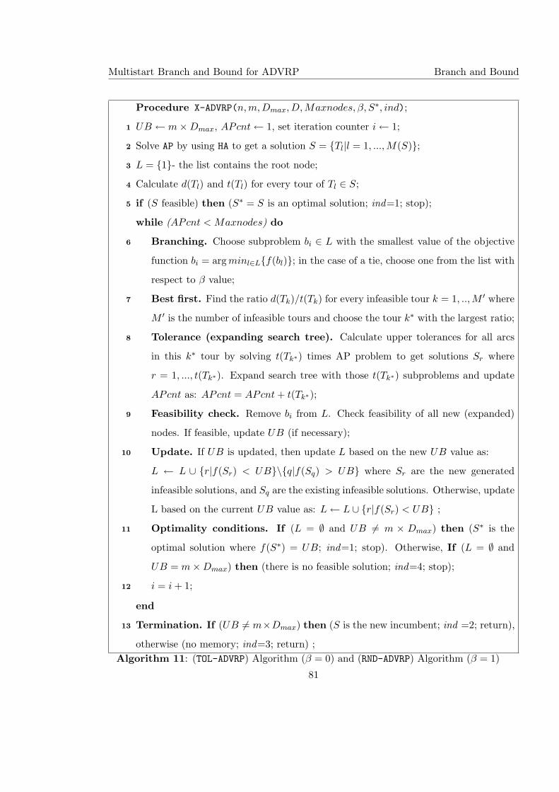
Multistart Branch and Bound for ADVRP Branch and Bound
Procedure X-ADVRP(n, m,Dmax, D,Maxnodes, β, S∗, ind);
UB ← m×Dmax, APcnt ← 1, set iteration counter i ← 1;1
Solve AP by using HA to get a solution S = {Tl|l = 1, ..., M(S)};2
L = {1}- the list contains the root node;3
Calculate d(Tl) and t(Tl) for every tour of Tl ∈ S;4
if (S feasible) then (S∗ = S is an optimal solution; ind=1; stop);5
while (APcnt < Maxnodes) do
Branching. Choose subproblem bi ∈ L with the smallest value of the objective6
function bi = arg minl∈L{f(bl)}; in the case of a tie, choose one from the list with
respect to β value;
Best first. Find the ratio d(Tk)/t(Tk) for every infeasible tour k = 1, .., M ′ where7
M ′ is the number of infeasible tours and choose the tour k∗ with the largest ratio;
Tolerance (expanding search tree). Calculate upper tolerances for all arcs8
in this k∗ tour by solving t(Tk∗) times AP problem to get solutions Sr where
r = 1, ..., t(Tk∗). Expand search tree with those t(Tk∗) subproblems and update
APcnt as: APcnt = APcnt + t(Tk∗);
Feasibility check. Remove bi from L. Check feasibility of all new (expanded)9
nodes. If feasible, update UB (if necessary);
Update. If UB is updated, then update L based on the new UB value as:10
L ← L ∪ {r|f(Sr) < UB}\{q|f(Sq) > UB} where Sr are the new generated
infeasible solutions, and Sq are the existing infeasible solutions. Otherwise, update
L based on the current UB value as: L ← L ∪ {r|f(Sr) < UB} ;
Optimality conditions. If (L = ∅ and UB 6= m × Dmax) then (S∗ is the11
optimal solution where f(S∗) = UB; ind=1; stop). Otherwise, If (L = ∅ and
UB = m×Dmax) then (there is no feasible solution; ind=4; stop);
i = i + 1;12
end
Termination. If (UB 6= m×Dmax) then (S is the new incumbent; ind =2; return),13
otherwise (no memory; ind=3; return) ;Algorithm 11: (TOL-ADVRP) Algorithm (β = 0) and (RND-ADVRP) Algorithm (β = 1)
81
Multistart Branch and Bound for ADVRP Branch and Bound
tolerance (UT) value to that arc. Note that the value of the counter APcnt is
increased by the number of arcs in the chosen tour:
APcnt = APcnt + t(Tk∗)
– Check Feasibility. Remove bi from L (L ← L\{bi}). Check feasibility of the
solution at every new generated subproblem.
– Update. If a feasible solution is found and its value is smaller than the current
upper bound, then update the value of the upper bound, update the list of active
subproblems by adding the new expanded subproblems that have value smaller
than UB and removing those subproblems that have value greater than UB as
follows:
L ← L ∪ {r|f(Sr) < UB}\{q|f(Sq) > UB}
Note that Sr are the new generated infeasible solutions, and Sq are the existing
infeasible solutions. Otherwise, i.e., if the upper bound is not updated, then
update L by adding the new expanded subproblems that have value smaller than
UB as follows:
L ← L ∪ {r|f(Sr) < UB}
– Optimality conditions. Check if L = ∅ and UB is updated then stop with the
value of optimal solution f(S∗) = UB (ind=1). Otherwise, if L = ∅ and UB is
not updated, stop with the message that no feasible solution exists (ind=4).
– Termination. When there is no memory we get two possible outputs:
∗ If UB is updated then S∗ is returned as feasible but not proven as the optimal
solution (ind=2).
∗ Otherwise, a feasible solution has not been found, but it might exist (ind=3).
Proposition 2 If there is no memory limit, then the algorithm TOL-ADVRP finds an optimal
solution to ADVRP or proves that such a solution does not exist.
82
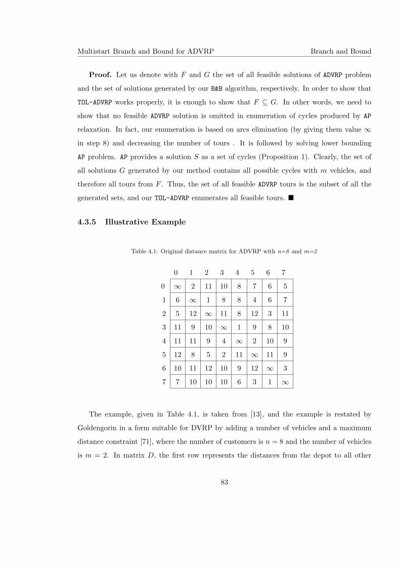
Multistart Branch and Bound for ADVRP Branch and Bound
Proof. Let us denote with F and G the set of all feasible solutions of ADVRP problem
and the set of solutions generated by our B&B algorithm, respectively. In order to show that
TOL-ADVRP works properly, it is enough to show that F ⊆ G. In other words, we need to
show that no feasible ADVRP solution is omitted in enumeration of cycles produced by AP
relaxation. In fact, our enumeration is based on arcs elimination (by giving them value ∞in step 8) and decreasing the number of tours . It is followed by solving lower bounding
AP problem. AP provides a solution S as a set of cycles (Proposition 1). Clearly, the set of
all solutions G generated by our method contains all possible cycles with m vehicles, and
therefore all tours from F . Thus, the set of all feasible ADVRP tours is the subset of all the
generated sets, and our TOL-ADVRP enumerates all feasible tours. ¥
4.3.5 Illustrative Example
Table 4.1: Original distance matrix for ADVRP with n=8 and m=2
0 1 2 3 4 5 6 7
0 ∞ 2 11 10 8 7 6 5
1 6 ∞ 1 8 8 4 6 7
2 5 12 ∞ 11 8 12 3 11
3 11 9 10 ∞ 1 9 8 10
4 11 11 9 4 ∞ 2 10 9
5 12 8 5 2 11 ∞ 11 9
6 10 11 12 10 9 12 ∞ 3
7 7 10 10 10 6 3 1 ∞
The example, given in Table 4.1, is taken from [13], and the example is restated by
Goldengorin in a form suitable for DVRP by adding a number of vehicles and a maximum
distance constraint [71], where the number of customers is n = 8 and the number of vehicles
is m = 2. In matrix D, the first row represents the distances from the depot to all other
83
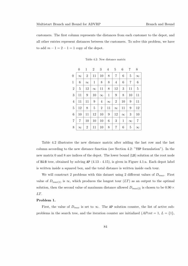
Multistart Branch and Bound for ADVRP Branch and Bound
customers. The first column represents the distances from each customer to the depot, and
all other entries represent distances between the customers. To solve this problem, we have
to add m− 1 = 2− 1 = 1 copy of the depot.
Table 4.2: New distance matrix
0 1 2 3 4 5 6 7 8
0 ∞ 2 11 10 8 7 6 5 ∞1 6 ∞ 1 8 8 4 6 7 6
2 5 12 ∞ 11 8 12 3 11 5
3 11 9 10 ∞ 1 9 8 10 11
4 11 11 9 4 ∞ 2 10 9 11
5 12 8 5 2 11 ∞ 11 9 12
6 10 11 12 10 9 12 ∞ 3 10
7 7 10 10 10 6 3 1 ∞ 7
8 ∞ 2 11 10 8 7 6 5 ∞
Table 4.2 illustrates the new distance matrix after adding the last row and the last
column according to the new distance function (see Section 4.2: ”TSP formulation”). In the
new matrix 0 and 8 are indices of the depot. The lower bound (LB) solution at the root node
of B&B tree, obtained by solving AP (4.13 - 4.15), is given in Figure 4.1:a. Each depot label
is written inside a squared box, and the total distance is written inside each tour.
We will construct 2 problems with this dataset using 2 different values of Dmax. First
value of Dmax(1) is ∞, which produces the longest tour (LT ) as an output to the optimal
solution, then the second value of maximum distance allowed Dmax(2) is chosen to be 0.90×LT .
Problem 1.
First, the value of Dmax is set to ∞. The AP solution counter, the list of active sub-
problems in the search tree, and the iteration counter are initialized (APcnt = 1, L = {1},
84
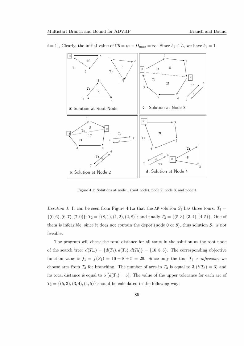
Multistart Branch and Bound for ADVRP Branch and Bound
i = 1), Clearly, the initial value of UB = m×Dmax = ∞. Since b1 ∈ L, we have b1 = 1.
Figure 4.1: Solutions at node 1 (root node), node 2, node 3, and node 4
Iteration 1. It can be seen from Figure 4.1:a that the AP solution S1 has three tours: T1 =
{(0, 6), (6, 7), (7, 0)}; T2 = {(8, 1), (1, 2), (2, 8)}; and finally T3 = {(5, 3), (3, 4), (4, 5)}. One of
them is infeasible, since it does not contain the depot (node 0 or 8), thus solution S1 is not
feasible.
The program will check the total distance for all tours in the solution at the root node
of the search tree: d(Tm) = {d(T1), d(T2), d(T3)} = {16, 8, 5}. The corresponding objective
function value is f1 = f(S1) = 16 + 8 + 5 = 29. Since only the tour T3 is infeasible, we
choose arcs from T3 for branching. The number of arcs in T3 is equal to 3 (t(T3) = 3) and
its total distance is equal to 5 (d(T3) = 5). The value of the upper tolerance for each arc of
T3 = {(5, 3), (3, 4), (4, 5)} should be calculated in the following way:
85
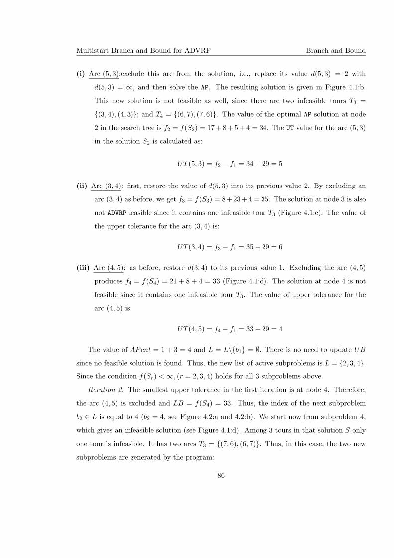
Multistart Branch and Bound for ADVRP Branch and Bound
(i) Arc (5, 3):exclude this arc from the solution, i.e., replace its value d(5, 3) = 2 with
d(5, 3) = ∞, and then solve the AP. The resulting solution is given in Figure 4.1:b.
This new solution is not feasible as well, since there are two infeasible tours T3 =
{(3, 4), (4, 3)}; and T4 = {(6, 7), (7, 6)}. The value of the optimal AP solution at node
2 in the search tree is f2 = f(S2) = 17 + 8 + 5 + 4 = 34. The UT value for the arc (5, 3)
in the solution S2 is calculated as:
UT (5, 3) = f2 − f1 = 34− 29 = 5
(ii) Arc (3, 4): first, restore the value of d(5, 3) into its previous value 2. By excluding an
arc (3, 4) as before, we get f3 = f(S3) = 8+23+4 = 35. The solution at node 3 is also
not ADVRP feasible since it contains one infeasible tour T3 (Figure 4.1:c). The value of
the upper tolerance for the arc (3, 4) is:
UT (3, 4) = f3 − f1 = 35− 29 = 6
(iii) Arc (4, 5): as before, restore d(3, 4) to its previous value 1. Excluding the arc (4, 5)
produces f4 = f(S4) = 21 + 8 + 4 = 33 (Figure 4.1:d). The solution at node 4 is not
feasible since it contains one infeasible tour T3. The value of upper tolerance for the
arc (4, 5) is:
UT (4, 5) = f4 − f1 = 33− 29 = 4
The value of APcnt = 1 + 3 = 4 and L = L\{b1} = ∅. There is no need to update UB
since no feasible solution is found. Thus, the new list of active subproblems is L = {2, 3, 4}.Since the condition f(Sr) < ∞, (r = 2, 3, 4) holds for all 3 subproblems above.
Iteration 2. The smallest upper tolerance in the first iteration is at node 4. Therefore,
the arc (4, 5) is excluded and LB = f(S4) = 33. Thus, the index of the next subproblem
b2 ∈ L is equal to 4 (b2 = 4, see Figure 4.2:a and 4.2:b). We start now from subproblem 4,
which gives an infeasible solution (see Figure 4.1:d). Among 3 tours in that solution S only
one tour is infeasible. It has two arcs T3 = {(7, 6), (6, 7)}. Thus, in this case, the two new
subproblems are generated by the program:
86
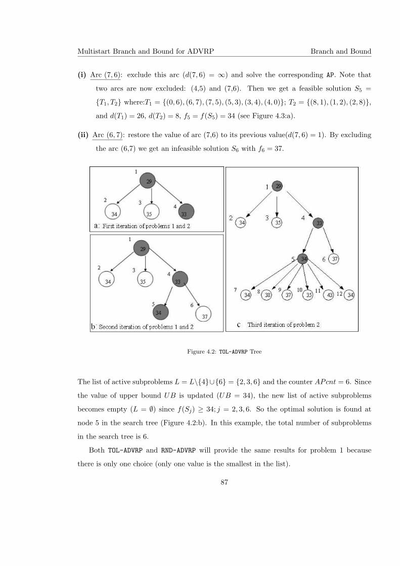
Multistart Branch and Bound for ADVRP Branch and Bound
(i) Arc (7, 6): exclude this arc (d(7, 6) = ∞) and solve the corresponding AP. Note that
two arcs are now excluded: (4,5) and (7,6). Then we get a feasible solution S5 =
{T1, T2} where:T1 = {(0, 6), (6, 7), (7, 5), (5, 3), (3, 4), (4, 0)}; T2 = {(8, 1), (1, 2), (2, 8)},and d(T1) = 26, d(T2) = 8, f5 = f(S5) = 34 (see Figure 4.3:a).
(ii) Arc (6, 7): restore the value of arc (7,6) to its previous value(d(7, 6) = 1). By excluding
the arc (6,7) we get an infeasible solution S6 with f6 = 37.
Figure 4.2: TOL-ADVRP Tree
The list of active subproblems L = L\{4}∪{6} = {2, 3, 6} and the counter APcnt = 6. Since
the value of upper bound UB is updated (UB = 34), the new list of active subproblems
becomes empty (L = ∅) since f(Sj) ≥ 34; j = 2, 3, 6. So the optimal solution is found at
node 5 in the search tree (Figure 4.2:b). In this example, the total number of subproblems
in the search tree is 6.
Both TOL-ADVRP and RND-ADVRP will provide the same results for problem 1 because
there is only one choice (only one value is the smallest in the list).
87
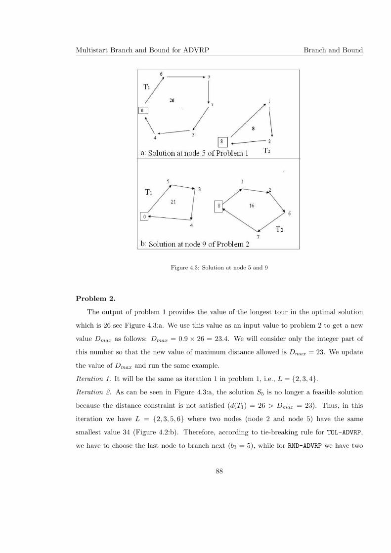
Multistart Branch and Bound for ADVRP Branch and Bound
Figure 4.3: Solution at node 5 and 9
Problem 2.
The output of problem 1 provides the value of the longest tour in the optimal solution
which is 26 see Figure 4.3:a. We use this value as an input value to problem 2 to get a new
value Dmax as follows: Dmax = 0.9 × 26 = 23.4. We will consider only the integer part of
this number so that the new value of maximum distance allowed is Dmax = 23. We update
the value of Dmax and run the same example.
Iteration 1. It will be the same as iteration 1 in problem 1, i.e., L = {2, 3, 4}.Iteration 2. As can be seen in Figure 4.3:a, the solution S5 is no longer a feasible solution
because the distance constraint is not satisfied (d(T1) = 26 > Dmax = 23). Thus, in this
iteration we have L = {2, 3, 5, 6} where two nodes (node 2 and node 5) have the same
smallest value 34 (Figure 4.2:b). Therefore, according to tie-breaking rule for TOL-ADVRP,
we have to choose the last node to branch next (b3 = 5), while for RND-ADVRP we have two
88
Multistart Branch and Bound for ADVRP Multistart Method
options node 2 and node 5, one of them will be chosen randomly. Assume node 5 is chosen
(b3 = 5). Node 5 has tow tours, one of them T1 is not feasible. Since T1 has 6 arcs then there
are 6 new subproblems generated in the search tree (see Figure 4.2:c). When we branch at
node 5, we find the first feasible solution at node 9, so we update UB = 37, APcnt = 12,
L = {2, 3, 7, 10, 12}.Iteration 3. In this iteration we have 3 nodes (2, 7, and 12) that have the same smallest value
34 (see Figure 4.2:c). For TOL-ADVRP, last node in the list has to be chosen to branch next i.e.,
b4 = 12, while for RND-ADVRP there are 3 options and one of them will be chosen randomly
(ns = 3). So we need to choose one k among three nodes: 2, 7 or 12 where k = 1 + 3α.
Assume that α = 0.4, then k = 2 and the second node b4 = 7 is chosen for branching. This
step is repeated at each iteration until the optimal solution is found or stopping conditions
is satisfied. At the end, after generating 58 subproblems (APcnt = 58) we get an optimal
solution value 37 (see Figure 4.3:b).
4.4 Multistart Method for ADVRP (MSBB-ADVRP)
The main idea of (RND-ADVRP) is to select randomly the next subproblem among those with
the same (smallest) objective function value. The random selection may cause the generation
of a smaller search tree. Therefore, if we reach the maximum number of subproblems allowed,
then the restart is required due to memory issues. Thus, we restart the exact B&B method
again, hoping that in the next attempt we will get an optimal solution. For that reason, in
MSBB-ADVRP we rerun RND-ADVRP (with β = 1) many times until an optimal solution is found
or infeasibility is proven. Each time we run RND-ADVRP, we save the value of UB as output
of RND-ADVRP (Note that we did not change the value of UB as input when RND-ADVRP is
rerun). Then we compare all the outputs of RND-ADVRP to keep the best as the output of
MSBB-ADVRP
4.4.1 Algorithm
The main points of (MSBB-ADVRP) algorithm 12 is summarized as follows:
89
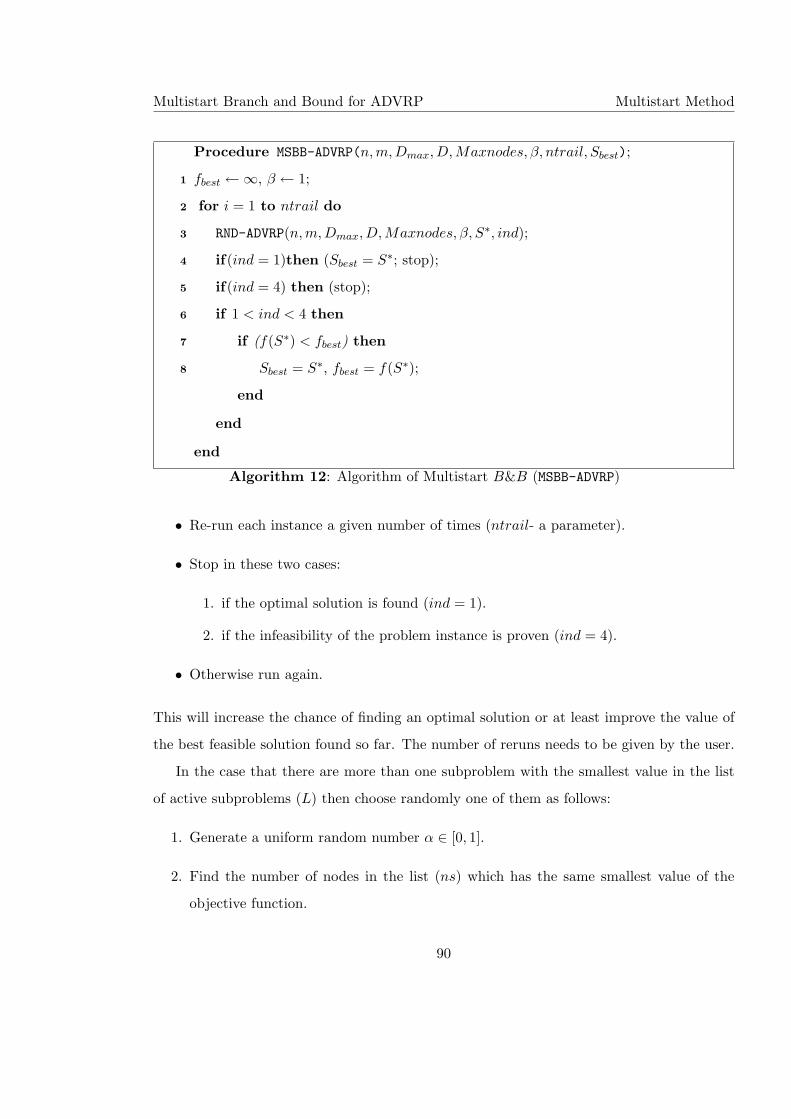
Multistart Branch and Bound for ADVRP Multistart Method
Procedure MSBB-ADVRP(n,m, Dmax, D,Maxnodes, β, ntrail, Sbest);
fbest ←∞, β ← 1;1
for i = 1 to ntrail do2
RND-ADVRP(n,m, Dmax, D, Maxnodes, β, S∗, ind);3
if(ind = 1)then (Sbest = S∗; stop);4
if(ind = 4) then (stop);5
if 1 < ind < 4 then6
if (f(S∗) < fbest) then7
Sbest = S∗, fbest = f(S∗);8
end
end
end
Algorithm 12: Algorithm of Multistart B&B (MSBB-ADVRP)
• Re-run each instance a given number of times (ntrail- a parameter).
• Stop in these two cases:
1. if the optimal solution is found (ind = 1).
2. if the infeasibility of the problem instance is proven (ind = 4).
• Otherwise run again.
This will increase the chance of finding an optimal solution or at least improve the value of
the best feasible solution found so far. The number of reruns needs to be given by the user.
In the case that there are more than one subproblem with the smallest value in the list
of active subproblems (L) then choose randomly one of them as follows:
1. Generate a uniform random number α ∈ [0, 1].
2. Find the number of nodes in the list (ns) which has the same smallest value of the
objective function.
90
Multistart Branch and Bound for ADVRP Implementation
3. Find k ∈ [1, ns] as k = 1 + ns ∗ α.
4. Branch on the node corresponding to the kth position.
In this thesis we set the parameter ntrail = 5, and it is called M5SBB-ADVRP.
Then we compare with RND-ADVRP to see what the improvement we get when we apply
a stochastic way of choosing from L and what the improvement we get when we rerun the
code 5 times.
4.4.2 Illustrative Example
We now present our MSBB-ADVRP on the same example from the previous section. We do not
consider Problem 1, since there were no ties.
Problem 2. We run the example with Dmax = 23.
Iteration 1. both programs do the same because we have only one smallest value in L (see
Figure 4.2:a).
Iteration 2. there are two nodes 2 and 5 that have the same smallest value f(S2) = f(S5) = 34
(Figure 4.2:b). So, there are two options and logically MSBB-ADVRP will provide two different
search trees. The outputs of applying MSBB-ADVRP in this case are as follows:
• if a first run provides an optimal solution, then no need to rerun the program again.
• if a first run provides a feasible solution, then rerun the program again. That could
find an optimal solution or at least produce another value of a feasible solution.
• if a first run is not able to find any feasible solution because no memory, so rerun
will give another chance to investigate another search tree and produce either proof of
infeasibility, or a feasible solution.
In general, there is a big chance to get two different values of best feasible solutions.
Iteration 3. the number of subproblems that have the same smallest value is equal to 3
(ns = 3). Therefore, there are 3 options, and MSBB-ADVRP will take benefit of that and
produce different outputs, hoping to reach an optimal solution. This step is repeated at each
iteration until the optimal solution is found or proof of infeasibility is found .
91
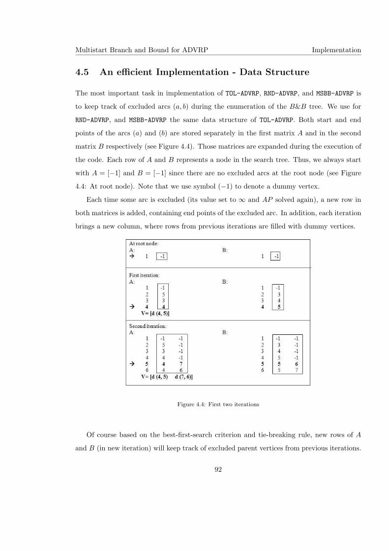
Multistart Branch and Bound for ADVRP Implementation
4.5 An efficient Implementation - Data Structure
The most important task in implementation of TOL-ADVRP, RND-ADVRP, and MSBB-ADVRP is
to keep track of excluded arcs (a, b) during the enumeration of the B&B tree. We use for
RND-ADVRP, and MSBB-ADVRP the same data structure of TOL-ADVRP. Both start and end
points of the arcs (a) and (b) are stored separately in the first matrix A and in the second
matrix B respectively (see Figure 4.4). Those matrices are expanded during the execution of
the code. Each row of A and B represents a node in the search tree. Thus, we always start
with A = [−1] and B = [−1] since there are no excluded arcs at the root node (see Figure
4.4: At root node). Note that we use symbol (−1) to denote a dummy vertex.
Each time some arc is excluded (its value set to ∞ and AP solved again), a new row in
both matrices is added, containing end points of the excluded arc. In addition, each iteration
brings a new column, where rows from previous iterations are filled with dummy vertices.
Figure 4.4: First two iterations
Of course based on the best-first-search criterion and tie-breaking rule, new rows of A
and B (in new iteration) will keep track of excluded parent vertices from previous iterations.
92
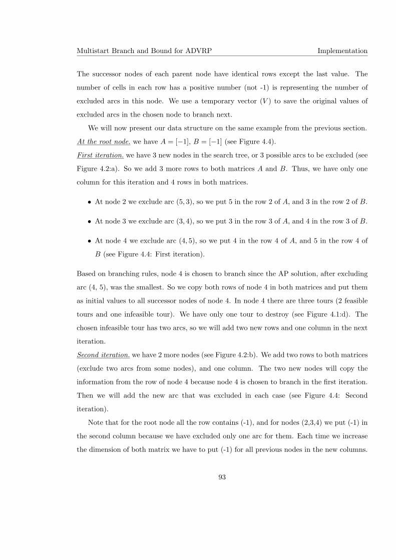
Multistart Branch and Bound for ADVRP Implementation
The successor nodes of each parent node have identical rows except the last value. The
number of cells in each row has a positive number (not -1) is representing the number of
excluded arcs in this node. We use a temporary vector (V ) to save the original values of
excluded arcs in the chosen node to branch next.
We will now present our data structure on the same example from the previous section.
At the root node. we have A = [−1], B = [−1] (see Figure 4.4).
First iteration. we have 3 new nodes in the search tree, or 3 possible arcs to be excluded (see
Figure 4.2:a). So we add 3 more rows to both matrices A and B. Thus, we have only one
column for this iteration and 4 rows in both matrices.
• At node 2 we exclude arc (5, 3), so we put 5 in the row 2 of A, and 3 in the row 2 of B.
• At node 3 we exclude arc (3, 4), so we put 3 in the row 3 of A, and 4 in the row 3 of B.
• At node 4 we exclude arc (4, 5), so we put 4 in the row 4 of A, and 5 in the row 4 of
B (see Figure 4.4: First iteration).
Based on branching rules, node 4 is chosen to branch since the AP solution, after excluding
arc (4, 5), was the smallest. So we copy both rows of node 4 in both matrices and put them
as initial values to all successor nodes of node 4. In node 4 there are three tours (2 feasible
tours and one infeasible tour). We have only one tour to destroy (see Figure 4.1:d). The
chosen infeasible tour has two arcs, so we will add two new rows and one column in the next
iteration.
Second iteration. we have 2 more nodes (see Figure 4.2:b). We add two rows to both matrices
(exclude two arcs from some nodes), and one column. The two new nodes will copy the
information from the row of node 4 because node 4 is chosen to branch in the first iteration.
Then we will add the new arc that was excluded in each case (see Figure 4.4: Second
iteration).
Note that for the root node all the row contains (-1), and for nodes (2,3,4) we put (-1) in
the second column because we have excluded only one arc for them. Each time we increase
the dimension of both matrix we have to put (-1) for all previous nodes in the new columns.
93
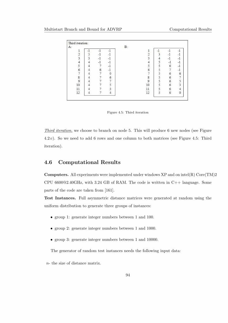
Multistart Branch and Bound for ADVRP Computational Results
Figure 4.5: Third iteration
Third iteration. we choose to branch on node 5. This will produce 6 new nodes (see Figure
4.2:c). So we need to add 6 rows and one column to both matrices (see Figure 4.5: Third
iteration).
4.6 Computational Results
Computers. All experiments were implemented under windows XP and on intel(R) Core(TM)2
CPU [email protected], with 3.24 GB of RAM. The code is written in C++ language. Some
parts of the code are taken from [161].
Test Instances. Full asymmetric distance matrices were generated at random using the
uniform distribution to generate three groups of instances:
• group 1: generate integer numbers between 1 and 100.
• group 2: generate integer numbers between 1 and 1000.
• group 3: generate integer numbers between 1 and 10000.
The generator of random test instances needs the following input data:
n- the size of distance matrix.
94
Multistart Branch and Bound for ADVRP Computational Results
γ- the parameter that controls the degree of symmetry in the distance matrix, γ ∈ [0, 1]: 0
means completely random and asymmetric; 1 means completely symmetric; 0.5 means
50% symmetric, etc.
seed - the random number: when n ≤ 200, four different distance matrices were generated
for each combination of (n,m). However, only one distance matrix is generated in the
case: 200 < n ≤ 1000.
The Floyd-Warshall Algorithm is used to calculate the shortest distance between all
vertices in the graph (for more information on the algorithm and the code see [154]). Ma-
trices satisfying triangle inequality C are obtained by applying Floyd-Warshall algorithm
on the generated matrices. Test instances are divided into two sets: small size (with
n = 40, 60, .., 200) and large size (with n = 240, 280, ..., 1000) instances. For each n be-
longing to the small set, two different types of instances are generated, based on the different
number of vehicles: m1 = n/20 and m2 = n/10. For instances belonging to the large set, we
use only m1.
In addition, for each distance matrix we consider 3 problems with 3 different values of
Dmax. The first value of Dmax(1) is set to ∞ and then we use this formulae to obtain the
new values of Dmax based on the length of the previous longest tour:
Dmax(i) = 0.90× LT (i− 1),
Where i ∈ {2, 3}, and LT (i − 1) is the longest tour in the optimal solution when the value
of the maximum distance allowed is Dmax(i−1). Note that we start with problem 1. If we
get optimal solution, then we continue to consider problem 2 otherwise we stop because we
could not obtain LT (1) to find Dmax(2), and so on.
The total number of instances in all groups are 695, distributed as follows: the first group
is 257; the second group is 222; and the third group is 216. All test instances used in this
thesis can be found on the following web site as well as the code for the generator coded in
C++: http://www.mi.sanu.ac.rs/∼nenad/advrp/
95
Multistart Branch and Bound for ADVRP Computational Results
4.6.1 Methods Compared.
In this thesis we compare three methods to find an optimal solution for ADVRP: MSBB-ADVRP,
TOL-ADVRP, CPLEX-ADVRP. In all our experiments reported below, MSBB-ADVRP use a random
tie-breaking rule. When MSBB-ADVRP runs the code once we get RND-ADVRP, while when it
reruns 5 times we get M5SS-ADVRP. We note that increasing the number of restarts might
improve the chances of finding an optimal solution, but with the cost of a larger CPU time.
In all methods the process will continue until one of these cases are met:
• an optimal solution is found.
• no memory.
• the time limit is reached.
We choose the time limit to be 10800 seconds (3 hours) for all test instances.
Comparison.
The rows in all tables give the following characteristics:
1. ] Opt (ind = 1)- how many times the optimal solution is found.
2. ] Feas (ind = 2) - how many times feasible (but not optimal) solutions have been
found.
3. ] No Mem (ind = 3) - how many times feasible solutions are not found because of lack
of memory.
4. ] No Feas (ind = 4) - how many instances with proven infeasibility are detected.
5. ] Feas=Opt - how many times feasible solutions have been found equal to optimal
solutions but without guarantee of optimality.
6. Total time (Opt)- the total time spent in seconds, only for instances where the optimal
solutions are found.
96
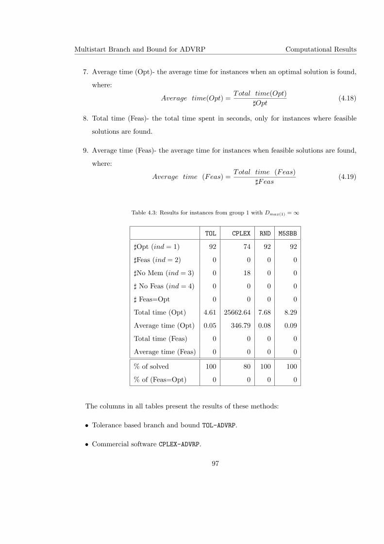
Multistart Branch and Bound for ADVRP Computational Results
7. Average time (Opt)- the average time for instances when an optimal solution is found,
where:
Average time(Opt) =Total time(Opt)
]Opt(4.18)
8. Total time (Feas)- the total time spent in seconds, only for instances where feasible
solutions are found.
9. Average time (Feas)- the average time for instances when feasible solutions are found,
where:
Average time (Feas) =Total time (Feas)
]Feas(4.19)
Table 4.3: Results for instances from group 1 with Dmax(1) = ∞
TOL CPLEX RND M5SBB
]Opt (ind = 1) 92 74 92 92
]Feas (ind = 2) 0 0 0 0
]No Mem (ind = 3) 0 18 0 0
] No Feas (ind = 4) 0 0 0 0
] Feas=Opt 0 0 0 0
Total time (Opt) 4.61 25662.64 7.68 8.29
Average time (Opt) 0.05 346.79 0.08 0.09
Total time (Feas) 0 0 0 0
Average time (Feas) 0 0 0 0
% of solved 100 80 100 100
% of (Feas=Opt) 0 0 0 0
The columns in all tables present the results of these methods:
• Tolerance based branch and bound TOL-ADVRP.
• Commercial software CPLEX-ADVRP.
97
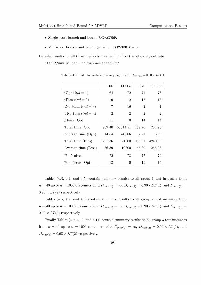
Multistart Branch and Bound for ADVRP Computational Results
• Single start branch and bound RND-ADVRP.
• Multistart branch and bound (ntrail = 5) M5SBB-ADVRP.
Detailed results for all three methods may be found on the following web site:
http://www.mi.sanu.ac.rs/∼nenad/advrp/.
Table 4.4: Results for instances from group 1 with Dmax(2) = 0.90× LT (1)
TOL CPLEX RND M5SBB
]Opt (ind = 1) 64 72 71 73
]Feas (ind = 2) 19 2 17 16
]No Mem (ind = 3) 7 16 2 1
] No Feas (ind = 4) 2 2 2 2
] Feas=Opt 11 0 14 14
Total time (Opt) 959.40 53644.51 157.26 261.75
Average time (Opt) 14.54 745.06 2.21 3.59
Total time (Feas) 1261.36 21600 958.61 4240.96
Average time (Feas) 66.39 10800 56.39 265.06
% of solved 72 78 77 79
% of (Feas=Opt) 12 0 15 15
Tables (4.3, 4.4, and 4.5) contain summary results to all group 1 test instances from
n = 40 up to n = 1000 customers with Dmax(1) = ∞, Dmax(2) = 0.90×LT (1), and Dmax(3) =
0.90× LT (2) respectively.
Tables (4.6, 4.7, and 4.8) contain summary results to all group 2 test instances from
n = 40 up to n = 1000 customers with Dmax(1) = ∞, Dmax(2) = 0.90×LT (1), and Dmax(3) =
0.90× LT (2) respectively.
Finally Tables (4.9, 4.10, and 4.11) contain summary results to all group 3 test instances
from n = 40 up to n = 1000 customers with Dmax(1) = ∞, Dmax(2) = 0.90 × LT (1), and
Dmax(3) = 0.90× LT (2) respectively.
98
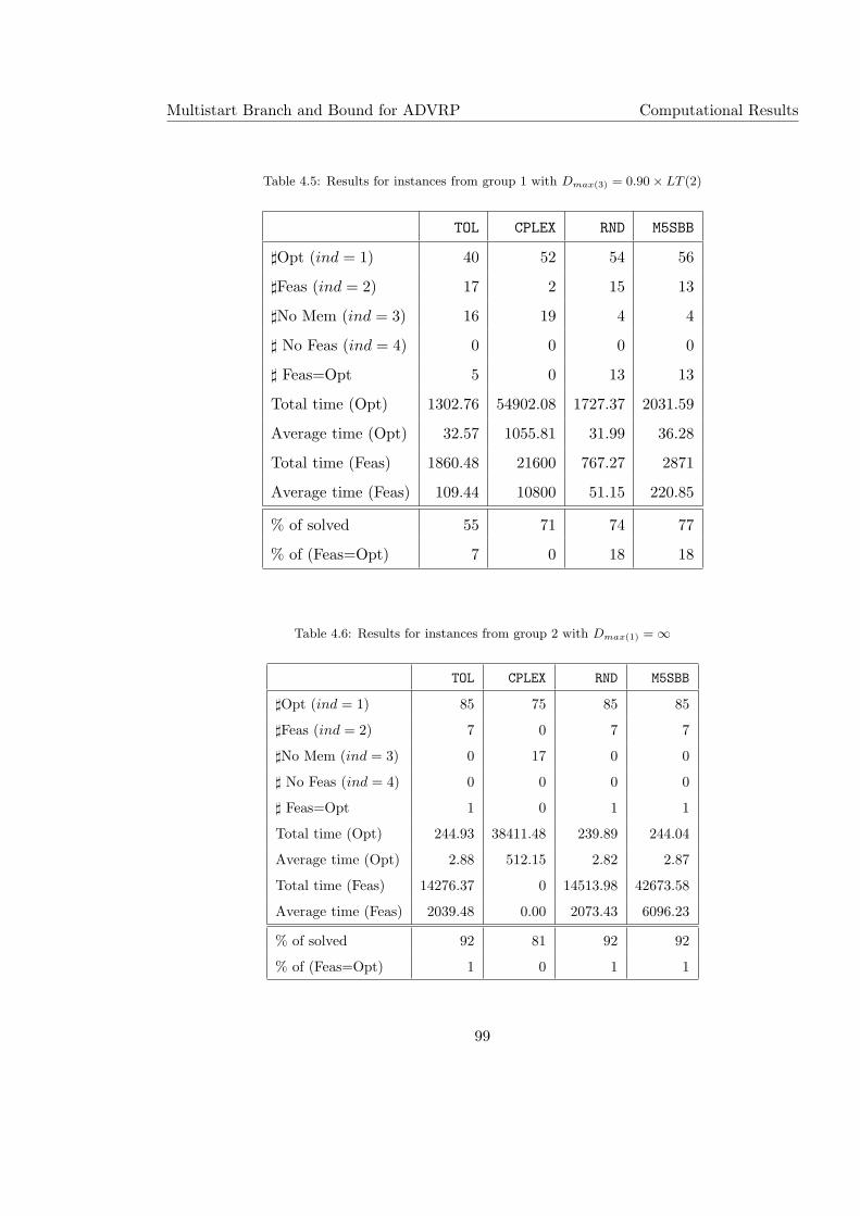
Multistart Branch and Bound for ADVRP Computational Results
Table 4.5: Results for instances from group 1 with Dmax(3) = 0.90× LT (2)
TOL CPLEX RND M5SBB
]Opt (ind = 1) 40 52 54 56
]Feas (ind = 2) 17 2 15 13
]No Mem (ind = 3) 16 19 4 4
] No Feas (ind = 4) 0 0 0 0
] Feas=Opt 5 0 13 13
Total time (Opt) 1302.76 54902.08 1727.37 2031.59
Average time (Opt) 32.57 1055.81 31.99 36.28
Total time (Feas) 1860.48 21600 767.27 2871
Average time (Feas) 109.44 10800 51.15 220.85
% of solved 55 71 74 77
% of (Feas=Opt) 7 0 18 18
Table 4.6: Results for instances from group 2 with Dmax(1) = ∞
TOL CPLEX RND M5SBB
]Opt (ind = 1) 85 75 85 85
]Feas (ind = 2) 7 0 7 7
]No Mem (ind = 3) 0 17 0 0
] No Feas (ind = 4) 0 0 0 0
] Feas=Opt 1 0 1 1
Total time (Opt) 244.93 38411.48 239.89 244.04
Average time (Opt) 2.88 512.15 2.82 2.87
Total time (Feas) 14276.37 0 14513.98 42673.58
Average time (Feas) 2039.48 0.00 2073.43 6096.23
% of solved 92 81 92 92
% of (Feas=Opt) 1 0 1 1
99

Multistart Branch and Bound for ADVRP Computational Results
Table 4.7: Results for instances from group 2 with Dmax(2) = 0.90× LT (1)
TOL CPLEX RND M5SBB
]Opt (ind = 1) 39 67 45 45
]Feas (ind = 2) 27 2 30 32
]No Mem (ind = 3) 17 14 8 6
] No Feas (ind = 4) 2 2 2 2
] Feas=Opt 13 0 16 18
Total time (Opt) 1487.57 34966.52 924.85 912.55
Average time (Opt) 38.14 521.89 20.55 20.28
Total time (Feas) 2183.82 21599.94 13529.43 45497.36
Average time (Feas) 80.88 10799.97 450.98 1421.79
% of solved 46 79 53 53
% of (Feas=Opt) 15 0 19 21
Table 4.8: Results for instances from group 2 with Dmax(3) = 0.90× LT (2)
TOL CPLEX RND M5SBB
]Opt (ind = 1) 16 34 27 28
]Feas (ind = 2) 13 2 14 13
]No Mem (ind = 3) 16 9 4 4
] No Feas (ind = 4) 0 0 0 0
] Feas=Opt 6 0 9 9
Total time (Opt) 577.69 21148.49 694.89 728.1
Average time (Opt) 36.11 622.01 25.74 26.00
Total time (Feas) 1762.68 21665.23 12990.62 28358.06
Average time (Feas) 135.59 10832.62 927.90 2181.39
% of solved 36 76 60 62
% of (Feas=Opt) 13 0 20 20
100
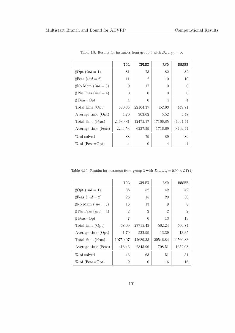
Multistart Branch and Bound for ADVRP Computational Results
Table 4.9: Results for instances from group 3 with Dmax(1) = ∞
TOL CPLEX RND M5SBB
]Opt (ind = 1) 81 73 82 82
]Feas (ind = 2) 11 2 10 10
]No Mem (ind = 3) 0 17 0 0
] No Feas (ind = 4) 0 0 0 0
] Feas=Opt 4 0 4 4
Total time (Opt) 380.35 22164.37 452.93 449.71
Average time (Opt) 4.70 303.62 5.52 5.48
Total time (Feas) 24689.81 12475.17 17166.85 34994.44
Average time (Feas) 2244.53 6237.59 1716.69 3499.44
% of solved 88 79 89 89
% of (Feas=Opt) 4 0 4 4
Table 4.10: Results for instances from group 3 with Dmax(2) = 0.90× LT (1)
TOL CPLEX RND M5SBB
]Opt (ind = 1) 38 52 42 42
]Feas (ind = 2) 26 15 29 30
]No Mem (ind = 3) 16 13 9 8
] No Feas (ind = 4) 2 2 2 2
] Feas=Opt 7 0 13 13
Total time (Opt) 68.09 27715.43 562.24 560.84
Average time (Opt) 1.79 532.99 13.39 13.35
Total time (Feas) 10750.07 42689.33 20546.84 49560.83
Average time (Feas) 413.46 2845.96 708.51 1652.03
% of solved 46 63 51 51
% of (Feas=Opt) 9 0 16 16
101
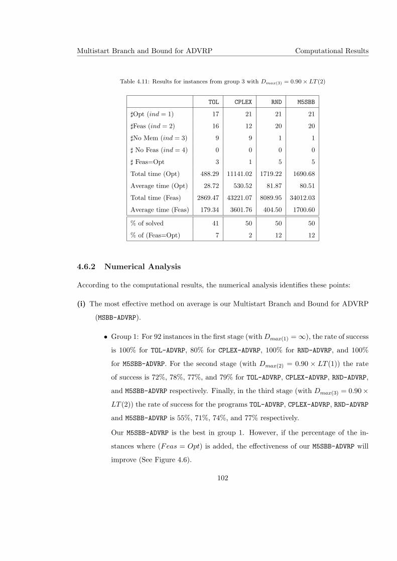
Multistart Branch and Bound for ADVRP Computational Results
Table 4.11: Results for instances from group 3 with Dmax(3) = 0.90× LT (2)
TOL CPLEX RND M5SBB
]Opt (ind = 1) 17 21 21 21
]Feas (ind = 2) 16 12 20 20
]No Mem (ind = 3) 9 9 1 1
] No Feas (ind = 4) 0 0 0 0
] Feas=Opt 3 1 5 5
Total time (Opt) 488.29 11141.02 1719.22 1690.68
Average time (Opt) 28.72 530.52 81.87 80.51
Total time (Feas) 2869.47 43221.07 8089.95 34012.03
Average time (Feas) 179.34 3601.76 404.50 1700.60
% of solved 41 50 50 50
% of (Feas=Opt) 7 2 12 12
4.6.2 Numerical Analysis
According to the computational results, the numerical analysis identifies these points:
(i) The most effective method on average is our Multistart Branch and Bound for ADVRP
(MSBB-ADVRP).
• Group 1: For 92 instances in the first stage (with Dmax(1) = ∞), the rate of success
is 100% for TOL-ADVRP, 80% for CPLEX-ADVRP, 100% for RND-ADVRP, and 100%
for M5SBB-ADVRP. For the second stage (with Dmax(2) = 0.90 × LT (1)) the rate
of success is 72%, 78%, 77%, and 79% for TOL-ADVRP, CPLEX-ADVRP, RND-ADVRP,
and M5SBB-ADVRP respectively. Finally, in the third stage (with Dmax(3) = 0.90×LT (2)) the rate of success for the programs TOL-ADVRP, CPLEX-ADVRP, RND-ADVRP
and M5SBB-ADVRP is 55%, 71%, 74%, and 77% respectively.
Our M5SBB-ADVRP is the best in group 1. However, if the percentage of the in-
stances where (Feas = Opt) is added, the effectiveness of our M5SBB-ADVRP will
improve (See Figure 4.6).
102
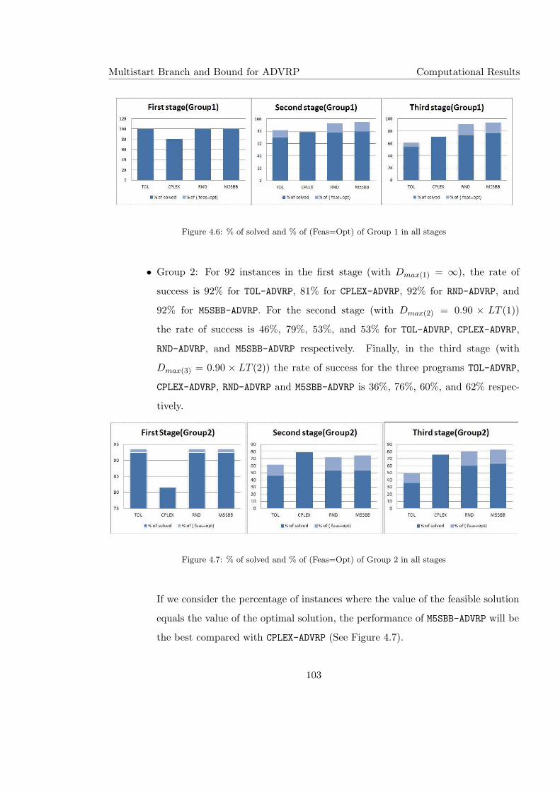
Multistart Branch and Bound for ADVRP Computational Results
Figure 4.6: % of solved and % of (Feas=Opt) of Group 1 in all stages
• Group 2: For 92 instances in the first stage (with Dmax(1) = ∞), the rate of
success is 92% for TOL-ADVRP, 81% for CPLEX-ADVRP, 92% for RND-ADVRP, and
92% for M5SBB-ADVRP. For the second stage (with Dmax(2) = 0.90 × LT (1))
the rate of success is 46%, 79%, 53%, and 53% for TOL-ADVRP, CPLEX-ADVRP,
RND-ADVRP, and M5SBB-ADVRP respectively. Finally, in the third stage (with
Dmax(3) = 0.90 × LT (2)) the rate of success for the three programs TOL-ADVRP,
CPLEX-ADVRP, RND-ADVRP and M5SBB-ADVRP is 36%, 76%, 60%, and 62% respec-
tively.
Figure 4.7: % of solved and % of (Feas=Opt) of Group 2 in all stages
If we consider the percentage of instances where the value of the feasible solution
equals the value of the optimal solution, the performance of M5SBB-ADVRP will be
the best compared with CPLEX-ADVRP (See Figure 4.7).
103
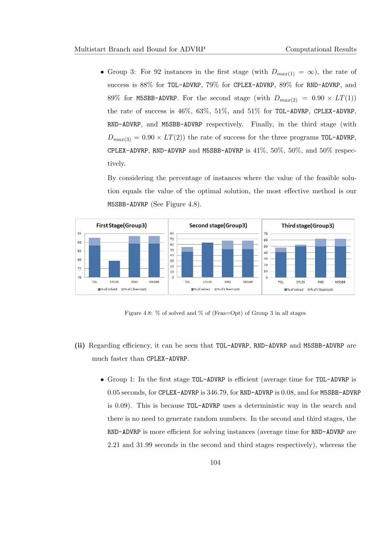
Multistart Branch and Bound for ADVRP Computational Results
• Group 3: For 92 instances in the first stage (with Dmax(1) = ∞), the rate of
success is 88% for TOL-ADVRP, 79% for CPLEX-ADVRP, 89% for RND-ADVRP, and
89% for M5SBB-ADVRP. For the second stage (with Dmax(2) = 0.90 × LT (1))
the rate of success is 46%, 63%, 51%, and 51% for TOL-ADVRP, CPLEX-ADVRP,
RND-ADVRP, and M5SBB-ADVRP respectively. Finally, in the third stage (with
Dmax(3) = 0.90 × LT (2)) the rate of success for the three programs TOL-ADVRP,
CPLEX-ADVRP, RND-ADVRP and M5SBB-ADVRP is 41%, 50%, 50%, and 50% respec-
tively.
By considering the percentage of instances where the value of the feasible solu-
tion equals the value of the optimal solution, the most effective method is our
M5SBB-ADVRP (See Figure 4.8).
Figure 4.8: % of solved and % of (Feas=Opt) of Group 3 in all stages
(ii) Regarding efficiency, it can be seen that TOL-ADVRP, RND-ADVRP and M5SBB-ADVRP are
much faster than CPLEX-ADVRP.
• Group 1: In the first stage TOL-ADVRP is efficient (average time for TOL-ADVRP is
0.05 seconds, for CPLEX-ADVRP is 346.79, for RND-ADVRP is 0.08, and for M5SBB-ADVRP
is 0.09). This is because TOL-ADVRP uses a deterministic way in the search and
there is no need to generate random numbers. In the second and third stages, the
RND-ADVRP is more efficient for solving instances (average time for RND-ADVRP are
2.21 and 31.99 seconds in the second and third stages respectively), whereas the
104
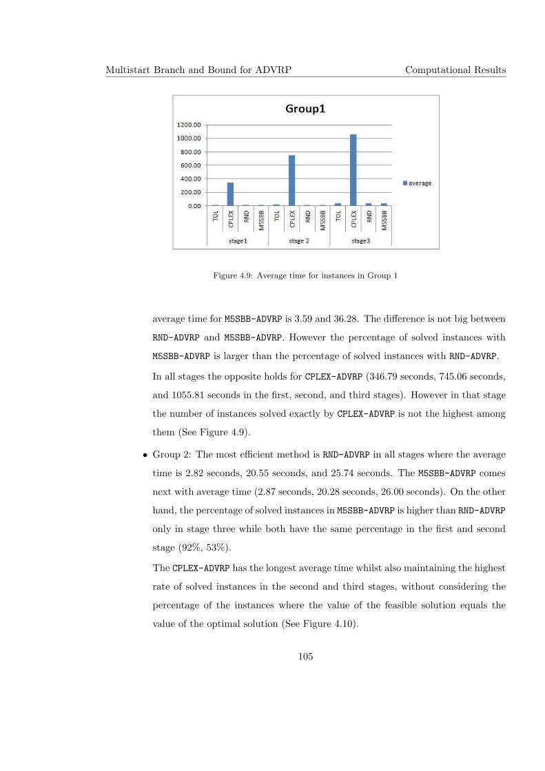
Multistart Branch and Bound for ADVRP Computational Results
Figure 4.9: Average time for instances in Group 1
average time for M5SBB-ADVRP is 3.59 and 36.28. The difference is not big between
RND-ADVRP and M5SBB-ADVRP. However the percentage of solved instances with
M5SBB-ADVRP is larger than the percentage of solved instances with RND-ADVRP.
In all stages the opposite holds for CPLEX-ADVRP (346.79 seconds, 745.06 seconds,
and 1055.81 seconds in the first, second, and third stages). However in that stage
the number of instances solved exactly by CPLEX-ADVRP is not the highest among
them (See Figure 4.9).
• Group 2: The most efficient method is RND-ADVRP in all stages where the average
time is 2.82 seconds, 20.55 seconds, and 25.74 seconds. The M5SBB-ADVRP comes
next with average time (2.87 seconds, 20.28 seconds, 26.00 seconds). On the other
hand, the percentage of solved instances in M5SBB-ADVRP is higher than RND-ADVRP
only in stage three while both have the same percentage in the first and second
stage (92%, 53%).
The CPLEX-ADVRP has the longest average time whilst also maintaining the highest
rate of solved instances in the second and third stages, without considering the
percentage of the instances where the value of the feasible solution equals the
value of the optimal solution (See Figure 4.10).
105
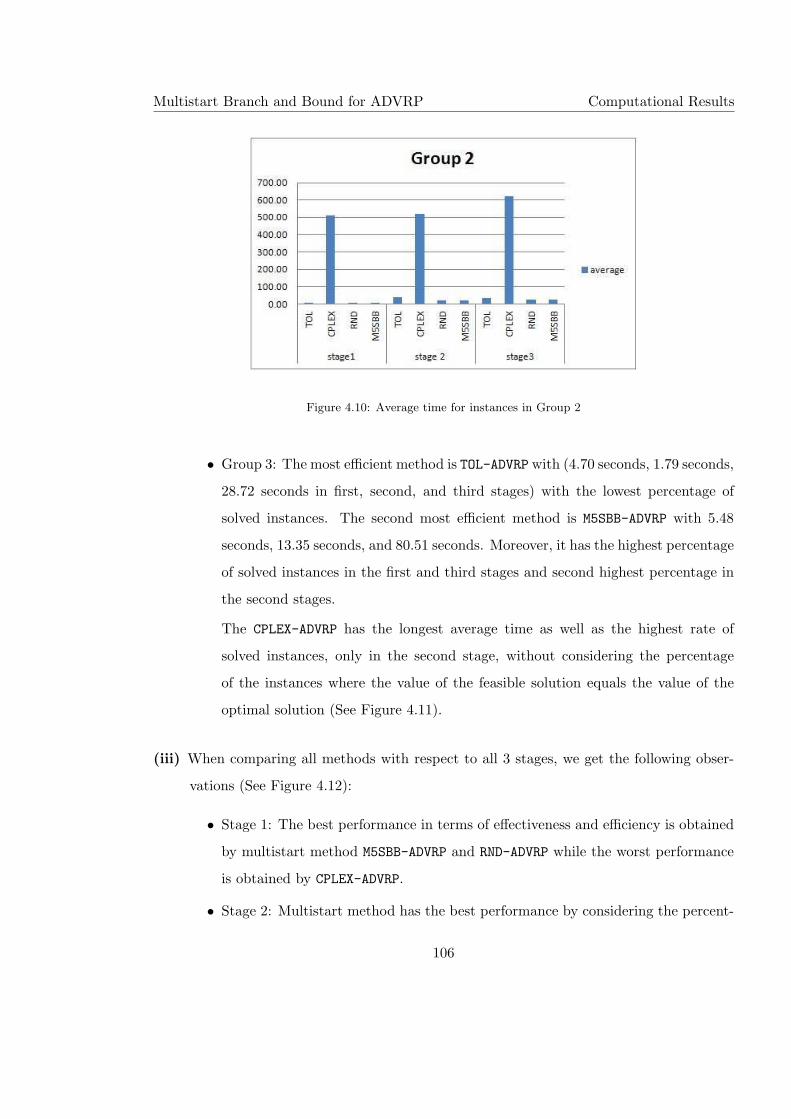
Multistart Branch and Bound for ADVRP Computational Results
Figure 4.10: Average time for instances in Group 2
• Group 3: The most efficient method is TOL-ADVRP with (4.70 seconds, 1.79 seconds,
28.72 seconds in first, second, and third stages) with the lowest percentage of
solved instances. The second most efficient method is M5SBB-ADVRP with 5.48
seconds, 13.35 seconds, and 80.51 seconds. Moreover, it has the highest percentage
of solved instances in the first and third stages and second highest percentage in
the second stages.
The CPLEX-ADVRP has the longest average time as well as the highest rate of
solved instances, only in the second stage, without considering the percentage
of the instances where the value of the feasible solution equals the value of the
optimal solution (See Figure 4.11).
(iii) When comparing all methods with respect to all 3 stages, we get the following obser-
vations (See Figure 4.12):
• Stage 1: The best performance in terms of effectiveness and efficiency is obtained
by multistart method M5SBB-ADVRP and RND-ADVRP while the worst performance
is obtained by CPLEX-ADVRP.
• Stage 2: Multistart method has the best performance by considering the percent-
106
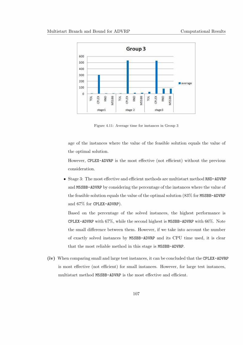
Multistart Branch and Bound for ADVRP Computational Results
Figure 4.11: Average time for instances in Group 3
age of the instances where the value of the feasible solution equals the value of
the optimal solution.
However, CPLEX-ADVRP is the most effective (not efficient) without the previous
consideration.
• Stage 3: The most effective and efficient methods are multistart method RND-ADVRP
and M5SBB-ADVRP by considering the percentage of the instances where the value of
the feasible solution equals the value of the optimal solution (83% for M5SBB-ADVRP
and 67% for CPLEX-ADVRP).
Based on the percentage of the solved instances, the highest performance is
CPLEX-ADVRP with 67%, while the second highest is M5SBB-ADVRP with 66%. Note
the small difference between them. However, if we take into account the number
of exactly solved instances by M5SBB-ADVRP and its CPU time used, it is clear
that the most reliable method in this stage is M5SBB-ADVRP.
(iv) When comparing small and large test instances, it can be concluded that the CPLEX-ADVRP
is most effective (not efficient) for small instances. However, for large test instances,
multistart method M5SBB-ADVRP is the most effective and efficient.
107
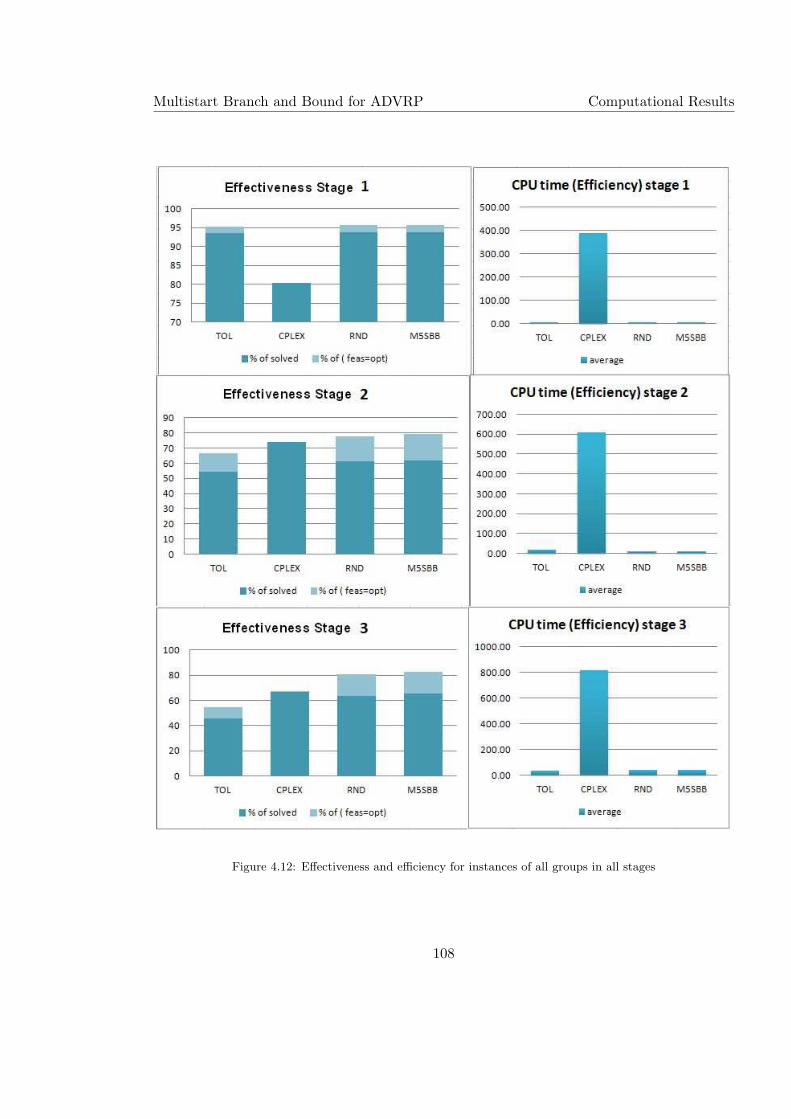
Multistart Branch and Bound for ADVRP Computational Results
Figure 4.12: Effectiveness and efficiency for instances of all groups in all stages
108
Multistart Branch and Bound for ADVRP Conclusion
4.7 Conclusion
We consider ADVRP and suggest exact algorithms for solving it. They are based on solv-
ing the Assignment problem relaxation and branching based on tolerances [6], where using
Assignment problem as relaxation to ADVRP was proposed for the first time by Laporte et.
al in 1987 [113]. We introduce a new method MSBB-ADVRP based on randomness in choosing
the next node in the branch and bound tree and restart the algorithm again and we compare
with CPLEX-ADVRP.
Computational experiments show that with our multistart approach MSBB-ADVRP we are
able to solve at least 77% in group 1, 53% in group 2, and 50% in group 3 of instances
in all stages with up to 1000 customers. while CPLEX-ADVRP is able to solve at least 71%,
76%, and 50% in group 1, group 2, and in group 3 respectively. It appears that MSBB-ADVRP
on average needs between 0.08 and 81.87 seconds, while CPLEX needs between 303.62 and
1055.81 seconds.
In summary, the results of experiments emphasize that using MSBB-ADVRP provides good
solutions in reasonable computational time. Moreover, as far as we know, we are able to
exactly solve problems with larger dimensions than previous methods in the literature. For
example the largest problem solved by CPLEX has n = 360 customers, while we are able
to solve exactly with n = 1000 customers. It is interesting to note that the dimensions of
problems solved by our methods depend on available memory of the computer used. Thus,
our approach may be used in the future using new computers with larger memory.
Real world instances are difficult to solve in our method. The reason is not a drawback of
our method but the lower bounding procedure (AP). These instances are clustered, making
it difficult to deal with because AP finds several subtours in the search tree, which deems
unhelpful in destroying one of them. Random instances do not have this property and we
prove computationally that our method outperforms other methods.
For future research, the running computational times of the algorithm can be improved
by developing a good heuristic such as Variable Neighborhood Search [85, 131], and to use
it as an initial upper bound. Another possibility is to improve lower bounds by adding
109
Multistart Branch and Bound for ADVRP Conclusion
more constraints to the assignment problem or to relax some of them using Lagrangian
multipliers. Such an approach does not use the advantages provided by fast Hungarian
method and could be a research topic for future work. Although we implement our B&B
based method on ADVRP problem, the method is quite general and may be adapted for
solving other VRP variants. Our approach is applied and tested on large instances. We are
proud to report that a good performance is achieved. We recommend our approach to be
applied on instances where symmetry does not exist.
110
Chapter 5
Variable Neighborhood Search for
ADVRP
Variable neighborhood search (VNS) is proposed by Mladenovic and Hansen in 1997 [131].
Its basic idea is to use different neighborhoods in order to move from a local optima towards
the global optima [77, 78, 79, 80, 81, 84, 87].
As mentioned before, our exact method (multi-start branch and bound) does not always
find a feasible solution and stops due to lack of memory. Moreover, for some large instances
when Dmax is tight, solving them can become harder and the exact method may stop before
it finds any feasible solution. For these reasons, in this chapter we develop a heuristic based
on VNS to find a good feasible solution in a short space of time.
The structure of this chapter is as follows: In section 5.1 we present two initialization
algorithms for ADVRP. Our VNS based heuristic for ADVRP is designed and explained
in section 5.2 with an illustrative example. Section 5.3 contains computational results and
finally in section 5.4 there is a conclusion.
5.1 Initialization Algorithms
We developed a code to solve ADVRP heuristically by using a VNS approach. We call our
heuristic VNS-ADVRP. As mentioned in Section 2.2, heuristics for solving VRP variants use
111
Variable Neighborhood Search Initialization Algorithms
two local search types: cluster-first-route-second, or route-first-cluster-second. We use in
this thesis route-first-cluster-second. Our heuristic VNS-ADVRP in its initialization step, calls
two subroutines: INIT-TSP and INIT-ADVRP.
5.1.1 INIT-TSP algorithm
INIT-TSP generates a few initial ATSP solutions and improves them. The INIT-TSP algo-
rithm is given in Algorithm 13 and its steps can be explained in the following way:
• build a random initial ATSP solution (RndPermut procedure).
• improve the initial solution by a well known local search (Swap procedure). It repeats
the following steps until no improvement is found or the number of iterations reaches
1000:
– exchange order of any two customers in the initial solution in a deterministic way;
calculate the value of the objective function. Assume there are n customers in the
ATSP tour, then there are n(n−1)2 possibilities for exchange. Each time 4 arcs are
added and 4 arcs are deleted at most. Finally choose the best swap between two
customers.
– if there is improvement, apply the best swap in the initial solution ATSP. Other-
wise, keep the current solution as it is.
Both RndPermut and Swap procedures are repeated a few times (10 times), the best
among them is chosen to be used as an input in the next step.
5.1.2 INIT-ADVRP Algorithm
INIT-ADVRP transforms ATSP solution to ADVRP solution and it has two stages:
• First stage:
– build (n− 1) solutions to ADVRP. The difference between solutions is the order
of the second vertex in the tour (i. e., the first customer), where the depot is
112
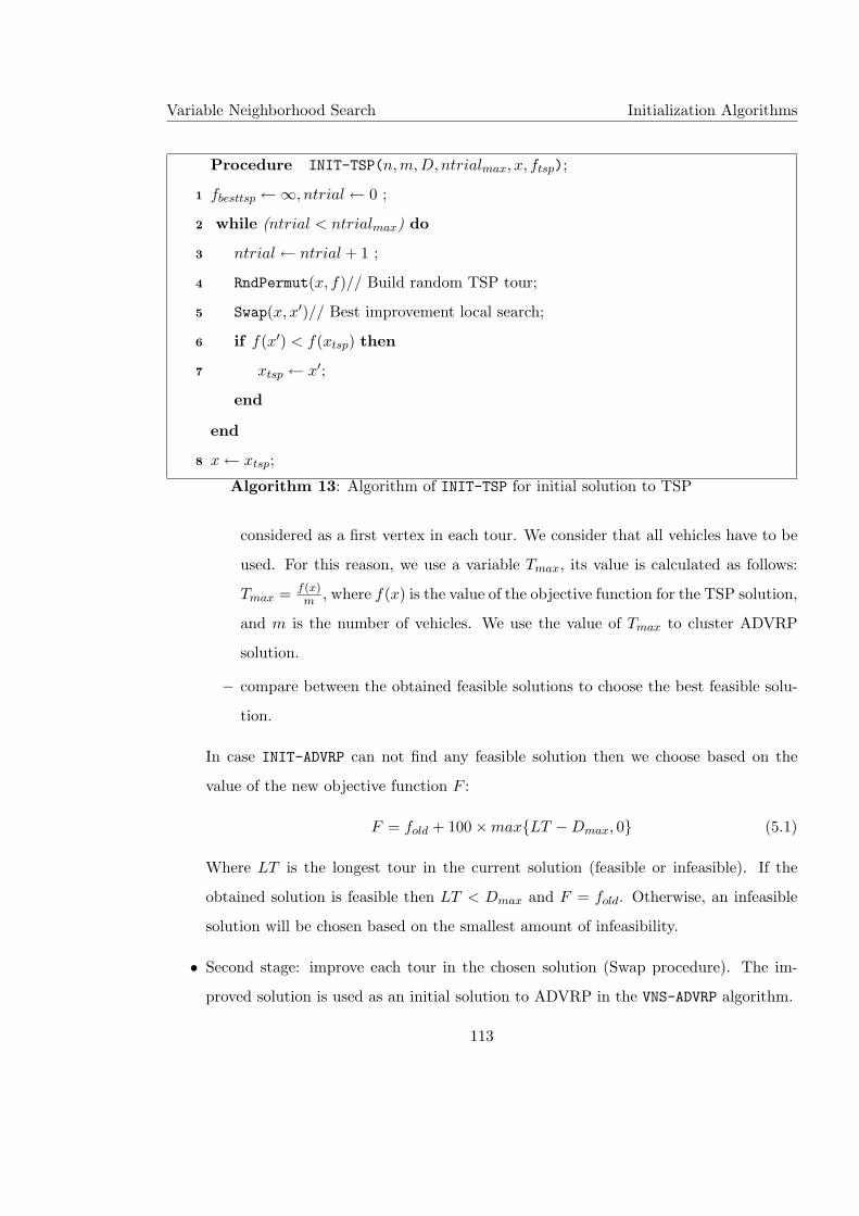
Variable Neighborhood Search Initialization Algorithms
Procedure INIT-TSP(n,m, D, ntrialmax, x, ftsp);
fbesttsp ←∞, ntrial ← 0 ;1
while (ntrial < ntrialmax) do2
ntrial ← ntrial + 1 ;3
RndPermut(x, f)// Build random TSP tour;4
Swap(x, x′)// Best improvement local search;5
if f(x′) < f(xtsp) then6
xtsp ← x′;7
end
end
x ← xtsp;8
Algorithm 13: Algorithm of INIT-TSP for initial solution to TSP
considered as a first vertex in each tour. We consider that all vehicles have to be
used. For this reason, we use a variable Tmax, its value is calculated as follows:
Tmax = f(x)m , where f(x) is the value of the objective function for the TSP solution,
and m is the number of vehicles. We use the value of Tmax to cluster ADVRP
solution.
– compare between the obtained feasible solutions to choose the best feasible solu-
tion.
In case INIT-ADVRP can not find any feasible solution then we choose based on the
value of the new objective function F :
F = fold + 100×max{LT −Dmax, 0} (5.1)
Where LT is the longest tour in the current solution (feasible or infeasible). If the
obtained solution is feasible then LT < Dmax and F = fold. Otherwise, an infeasible
solution will be chosen based on the smallest amount of infeasibility.
• Second stage: improve each tour in the chosen solution (Swap procedure). The im-
proved solution is used as an initial solution to ADVRP in the VNS-ADVRP algorithm.
113
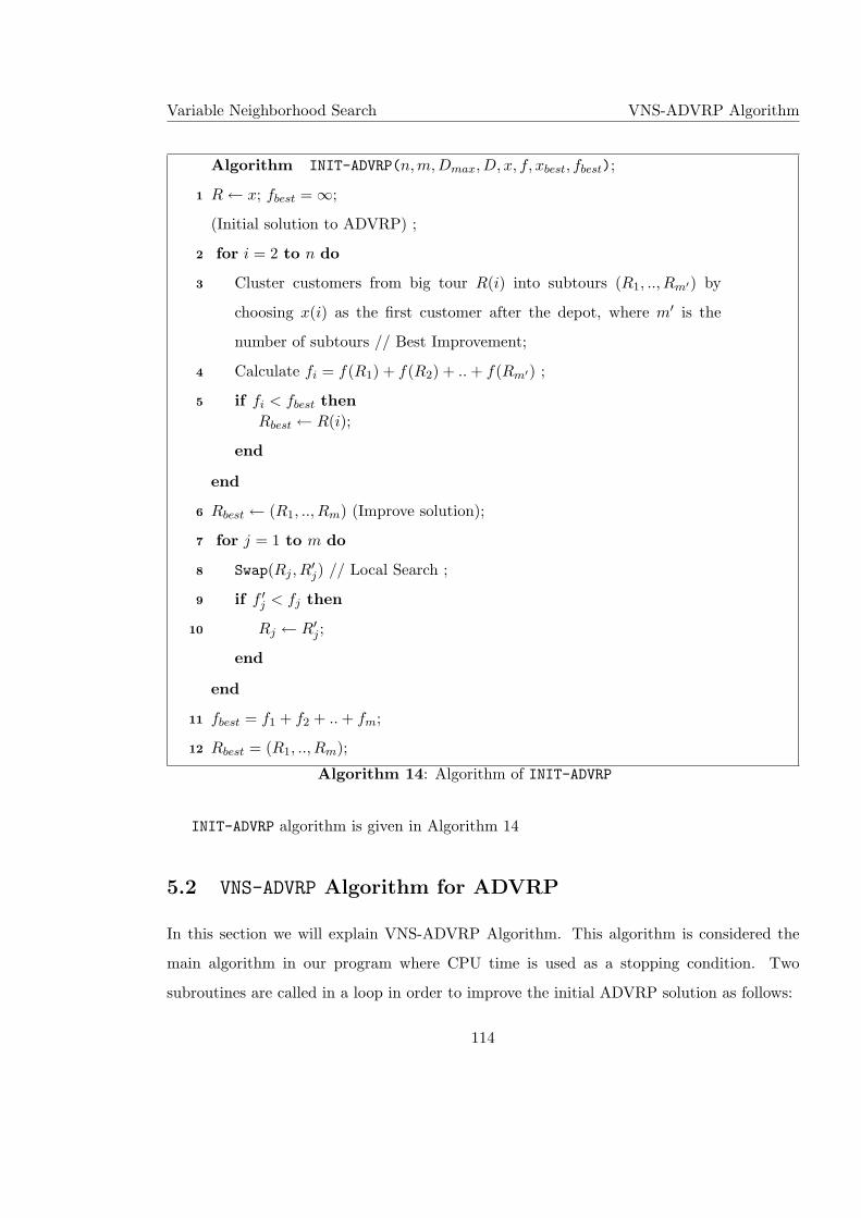
Variable Neighborhood Search VNS-ADVRP Algorithm
Algorithm INIT-ADVRP(n,m, Dmax, D, x, f, xbest, fbest);
R ← x; fbest = ∞;1
(Initial solution to ADVRP) ;
for i = 2 to n do2
Cluster customers from big tour R(i) into subtours (R1, .., Rm′) by3
choosing x(i) as the first customer after the depot, where m′ is the
number of subtours // Best Improvement;
Calculate fi = f(R1) + f(R2) + .. + f(Rm′) ;4
if fi < fbest then5
Rbest ← R(i);
end
end
Rbest ← (R1, .., Rm) (Improve solution);6
for j = 1 to m do7
Swap(Rj , R′j) // Local Search ;8
if f ′j < fj then9
Rj ← R′j ;10
end
end
fbest = f1 + f2 + .. + fm;11
Rbest = (R1, .., Rm);12
Algorithm 14: Algorithm of INIT-ADVRP
INIT-ADVRP algorithm is given in Algorithm 14
5.2 VNS-ADVRP Algorithm for ADVRP
In this section we will explain VNS-ADVRP Algorithm. This algorithm is considered the
main algorithm in our program where CPU time is used as a stopping condition. Two
subroutines are called in a loop in order to improve the initial ADVRP solution as follows:
114
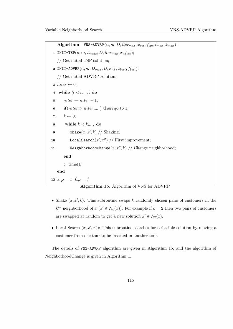
Variable Neighborhood Search VNS-ADVRP Algorithm
Algorithm VNS-ADVRP(n,m, D, itermax, xopt, fopt, tmax, kmax);
INIT-TSP(n,m, Dmax, D, itermax, x, ftsp);1
// Get initial TSP solution;
INIT-ADVRP(n,m, Dmax, D, x, f, xbest, fbest);2
// Get initial ADVRP solution;
niter ← 0;3
while (t < tmax) do4
niter ← niter + 1;5
if(niter > nitermax) then go to 1;6
k ← 0;7
while k < kmax do8
Shake(x, x′, k) // Shaking;9
LocalSearch(x′, x′′) // First improvement;10
NeighborhoodChange(x, x′′, k) // Change neighborhood;11
end
t=time();
end
xopt = x, fopt = f12
Algorithm 15: Algorithm of VNS for ADVRP
• Shake (x, x′, k): This subroutine swaps k randomly chosen pairs of customers in the
kth neighborhood of x (x′ ∈ Nk(x)). For example if k = 2 then two pairs of customers
are swapped at random to get a new solution x′ ∈ N2(x).
• Local Search (x, x′, x′′): This subroutine searches for a feasible solution by moving a
customer from one tour to be inserted in another tour.
The details of VNS-ADVRP algorithm are given in Algorithm 15, and the algorithm of
NeighborhoodChange is given in Algorithm 1.
115
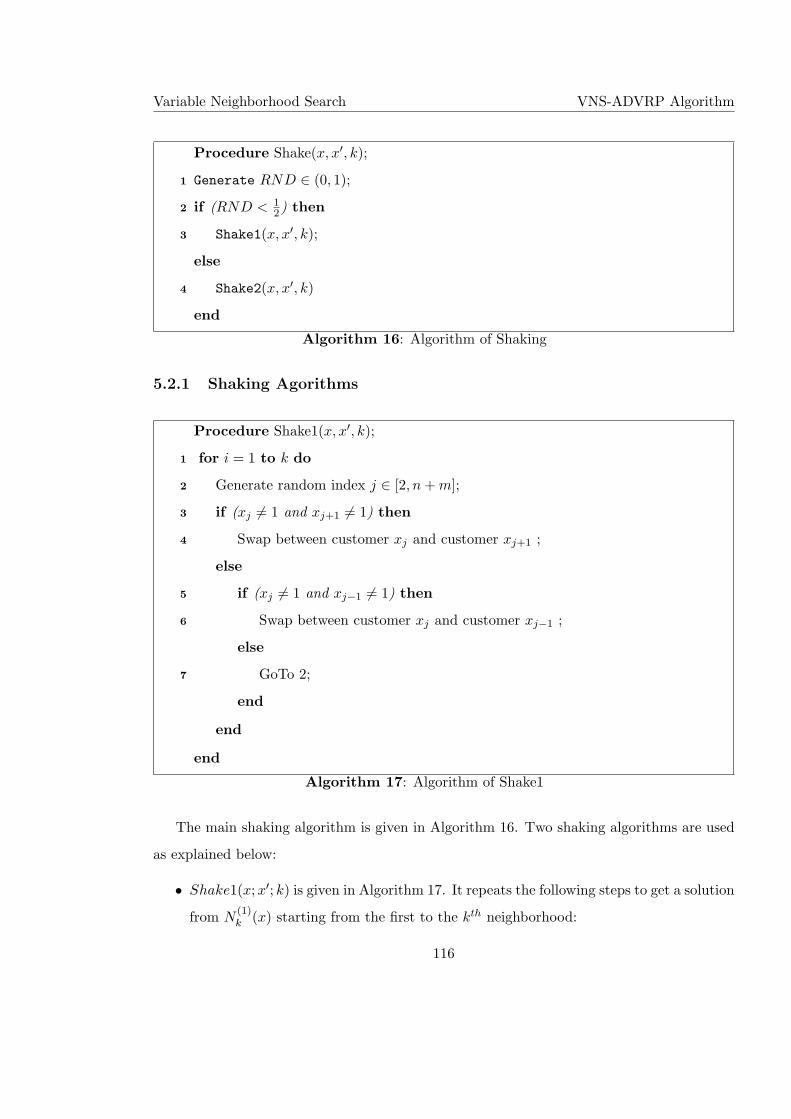
Variable Neighborhood Search VNS-ADVRP Algorithm
Procedure Shake(x, x′, k);
Generate RND ∈ (0, 1);1
if (RND < 12) then2
Shake1(x, x′, k);3
else
Shake2(x, x′, k)4
end
Algorithm 16: Algorithm of Shaking
5.2.1 Shaking Agorithms
Procedure Shake1(x, x′, k);
for i = 1 to k do1
Generate random index j ∈ [2, n + m];2
if (xj 6= 1 and xj+1 6= 1) then3
Swap between customer xj and customer xj+1 ;4
else
if (xj 6= 1 and xj−1 6= 1) then5
Swap between customer xj and customer xj−1 ;6
else
GoTo 2;7
end
end
end
Algorithm 17: Algorithm of Shake1
The main shaking algorithm is given in Algorithm 16. Two shaking algorithms are used
as explained below:
• Shake1(x;x′; k) is given in Algorithm 17. It repeats the following steps to get a solution
from N(1)k (x) starting from the first to the kth neighborhood:
116
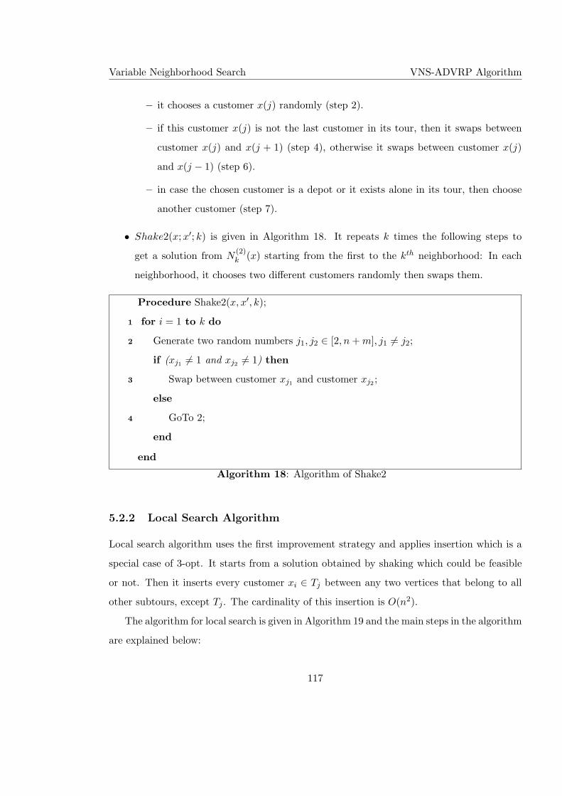
Variable Neighborhood Search VNS-ADVRP Algorithm
– it chooses a customer x(j) randomly (step 2).
– if this customer x(j) is not the last customer in its tour, then it swaps between
customer x(j) and x(j + 1) (step 4), otherwise it swaps between customer x(j)
and x(j − 1) (step 6).
– in case the chosen customer is a depot or it exists alone in its tour, then choose
another customer (step 7).
• Shake2(x;x′; k) is given in Algorithm 18. It repeats k times the following steps to
get a solution from N(2)k (x) starting from the first to the kth neighborhood: In each
neighborhood, it chooses two different customers randomly then swaps them.
Procedure Shake2(x, x′, k);
for i = 1 to k do1
Generate two random numbers j1, j2 ∈ [2, n + m], j1 6= j2;2
if (xj1 6= 1 and xj2 6= 1) then
Swap between customer xj1 and customer xj2 ;3
else
GoTo 2;4
end
end
Algorithm 18: Algorithm of Shake2
5.2.2 Local Search Algorithm
Local search algorithm uses the first improvement strategy and applies insertion which is a
special case of 3-opt. It starts from a solution obtained by shaking which could be feasible
or not. Then it inserts every customer xi ∈ Tj between any two vertices that belong to all
other subtours, except Tj . The cardinality of this insertion is O(n2).
The algorithm for local search is given in Algorithm 19 and the main steps in the algorithm
are explained below:
117
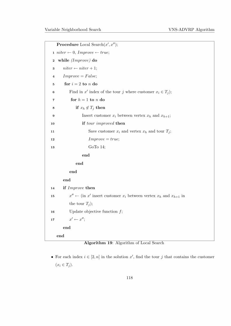
Variable Neighborhood Search VNS-ADVRP Algorithm
Procedure Local Search(x′, x′′);
niter ← 0, Improve ← true;1
while (Improve) do2
niter ← niter + 1;3
Improve = False;4
for i = 2 to n do5
Find in x′ index of the tour j where customer xi ∈ Tj);6
for h = 1 to n do7
if xh 6∈ Tj then8
Insert customer xi between vertex xh and xh+1;9
if tour improved then10
Save customer xi and vertex xh and tour Tj ;11
Improve = true;12
GoTo 14;13
end
end
end
end
if Improve then14
x′′ ← (in x′ insert customer xi between vertex xh and xh+1 in15
the tour Tj);
Update objective function f ;16
x′ ← x′′;17
end
end
Algorithm 19: Algorithm of Local Search
• For each index i ∈ [2, n] in the solution x′, find the tour j that contains the customer
(xi ∈ Tj).
118
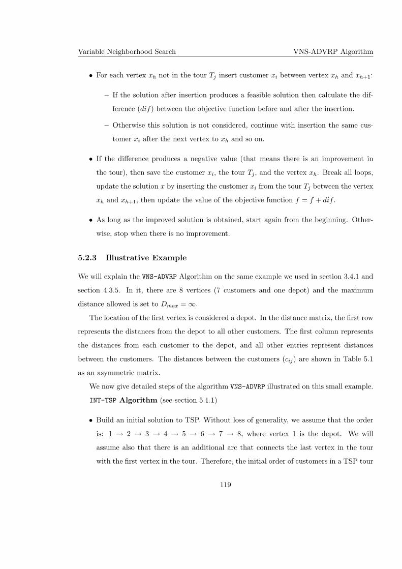
Variable Neighborhood Search VNS-ADVRP Algorithm
• For each vertex xh not in the tour Tj insert customer xi between vertex xh and xh+1:
– If the solution after insertion produces a feasible solution then calculate the dif-
ference (dif) between the objective function before and after the insertion.
– Otherwise this solution is not considered, continue with insertion the same cus-
tomer xi after the next vertex to xh and so on.
• If the difference produces a negative value (that means there is an improvement in
the tour), then save the customer xi, the tour Tj , and the vertex xh. Break all loops,
update the solution x by inserting the customer xi from the tour Tj between the vertex
xh and xh+1, then update the value of the objective function f = f + dif .
• As long as the improved solution is obtained, start again from the beginning. Other-
wise, stop when there is no improvement.
5.2.3 Illustrative Example
We will explain the VNS-ADVRP Algorithm on the same example we used in section 3.4.1 and
section 4.3.5. In it, there are 8 vertices (7 customers and one depot) and the maximum
distance allowed is set to Dmax = ∞.
The location of the first vertex is considered a depot. In the distance matrix, the first row
represents the distances from the depot to all other customers. The first column represents
the distances from each customer to the depot, and all other entries represent distances
between the customers. The distances between the customers (cij) are shown in Table 5.1
as an asymmetric matrix.
We now give detailed steps of the algorithm VNS-ADVRP illustrated on this small example.
INT-TSP Algorithm (see section 5.1.1)
• Build an initial solution to TSP. Without loss of generality, we assume that the order
is: 1 → 2 → 3 → 4 → 5 → 6 → 7 → 8, where vertex 1 is the depot. We will
assume also that there is an additional arc that connects the last vertex in the tour
with the first vertex in the tour. Therefore, the initial order of customers in a TSP tour
119
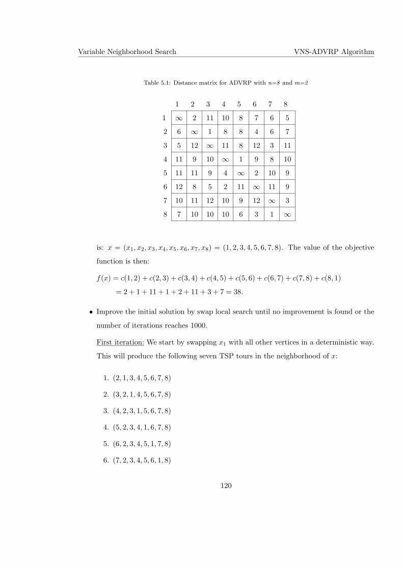
Variable Neighborhood Search VNS-ADVRP Algorithm
Table 5.1: Distance matrix for ADVRP with n=8 and m=2
1 2 3 4 5 6 7 8
1 ∞ 2 11 10 8 7 6 5
2 6 ∞ 1 8 8 4 6 7
3 5 12 ∞ 11 8 12 3 11
4 11 9 10 ∞ 1 9 8 10
5 11 11 9 4 ∞ 2 10 9
6 12 8 5 2 11 ∞ 11 9
7 10 11 12 10 9 12 ∞ 3
8 7 10 10 10 6 3 1 ∞
is: x = (x1, x2, x3, x4, x5, x6, x7, x8) = (1, 2, 3, 4, 5, 6, 7, 8). The value of the objective
function is then:
f(x) = c(1, 2) + c(2, 3) + c(3, 4) + c(4, 5) + c(5, 6) + c(6, 7) + c(7, 8) + c(8, 1)
= 2 + 1 + 11 + 1 + 2 + 11 + 3 + 7 = 38.
• Improve the initial solution by swap local search until no improvement is found or the
number of iterations reaches 1000.
First iteration: We start by swapping x1 with all other vertices in a deterministic way.
This will produce the following seven TSP tours in the neighborhood of x:
1. (2, 1, 3, 4, 5, 6, 7, 8)
2. (3, 2, 1, 4, 5, 6, 7, 8)
3. (4, 2, 3, 1, 5, 6, 7, 8)
4. (5, 2, 3, 4, 1, 6, 7, 8)
5. (6, 2, 3, 4, 5, 1, 7, 8)
6. (7, 2, 3, 4, 5, 6, 1, 8)
120
Variable Neighborhood Search VNS-ADVRP Algorithm
7. (8, 2, 3, 4, 5, 6, 7, 1)
Continue swapping xi with all other vertices xj except with {xj |j < i} in a deterministic
way, to get the remaining TSP tours. At the end, there will be n(n−1)2 possible TSP
tours. Since n = 8, there will be 28 TSP tours in N1 neighborhood of x.
N1(x) = {(2, 1, 3, 4, 5, 6, 7, 8), (3, 2, 1, 4, 5, 6, 7, 8), (4, 2, 3, 1, 5, 6, 7, 8), (5, 2, 3, 4, 1, 6, 7, 8),
(6, 2, 3, 4, 5, 1, 7, 8), (7, 2, 3, 4, 5, 6, 1, 8), (8, 2, 3, 4, 5, 6, 7, 1), (1, 3, 2, 4, 5, 6, 7, 8),
(1, 4, 3, 2, 5, 6, 7, 8), (1, 5, 3, 4, 2, 6, 7, 8), (1, 6, 3, 4, 5, 2, 7, 8), (1, 7, 3, 4, 5, 6, 2, 8),
(1, 8, 3, 4, 5, 6, 7, 2), (1, 2, 4, 3, 5, 6, 7, 8), (1, 2, 5, 4, 3, 6, 7, 8), (1, 2, 6, 4, 5, 3, 7, 8),
(1, 2, 7, 4, 5, 6, 3, 8), (1, 2, 8, 4, 5, 6, 7, 3), (1, 2, 3, 5, 4, 6, 7, 8), (1, 2, 3, 6, 5, 4, 7, 8),
(1, 2, 3, 7, 5, 6, 4, 8), (1, 2, 3, 8, 5, 6, 7, 4), (1, 2, 3, 4, 6, 5, 7, 8), (1, 2, 3, 4, 7, 6, 5, 8),
(1, 2, 3, 4, 8, 6, 7, 5), (1, 2, 3, 4, 5, 7, 6, 8), (1, 2, 3, 4, 5, 8, 7, 6), (1, 2, 3, 4, 5, 6, 8, 7)}.
The difference in the value of the objective function before and after the swap is
calculated by adding the length of the new arcs and subtracting the length of the
deleted arcs. The current TSP tour is: x = (1, 2, 3, 4, 5, 6, 7, 8). If we swap x1 and
x2 then we get x1 = (2, 1, 3, 4, 5, 6, 7, 8), the difference ∆1 between f(x1) and f(x) is
calculated as follows:
∆1 = c(8, 2) + c(2, 1) + c(1, 3)− c(1, 2)− c(2, 3)− c(8, 1)
= 10 + 6 + 11− 2− 1− 7 = 17.
If we get a negative number, the improved value of the objective function is obtained.
Otherwise, the swap is not useful since the value of the objective function is increased.
Each time two vertices (xi, xk) are swapped, the value of ∆j(j = 1, ..., 28) is calculated.
We keep the smallest value of ∆ = min{∆j |j = 1, ..., 28} which corresponds to the
best swap. In this example the value of ∆ is equal to −7 and it corresponds to
the swap between x3 and x6 in x. Therefore, the new incumbent solution is x′ =
(1, 2, 6, 4, 5, 3, 7, 8), where f(x′) = f(x) + ∆ = 38 − 7 = 31. Set x = x′ and use it as
the new best solution.
Second iteration: In the second iteration, we get ∆ = 4, so the local minimum with
respect to 1-swap neighborhood is reached and we stop local search since we get the
121
Variable Neighborhood Search VNS-ADVRP Algorithm
local minimum x = (1, 2, 6, 4, 5, 3, 7, 8) with the objective function value f(x) = 31.
In INT-TSP Algorithm, we generate 10 random initial TSP tours and we try to improve each
of them by local search. We choose the best local minimum obtained. Note that we do not
get the same tour in each run of the code since it depends on the random initial tour. The
best tour we found in 10 restarts is: x = (1, 2, 3, 7, 8, 6, 4, 5) and the value of the objective
function is 26. This TSP tour is then used as an input of the next initialization algorithm
(INIT-ADVRP Algorithm) to find the best initial DVRP solution.
INIT-ADVRP Algorithm (see section 5.1.2)
The best obtained TSP tour is x = (1, 2, 3, 7, 8, 6, 4, 5). This algorithm has two stages:
• First stage: we build n − 1 = 8 − 1 = 7 solutions to DVRP. The value of Tmaxis
calculated as follows: Tmax = f(x)m = 26
2 = 13. We use the value of Tmax to cluster
ADVRP tours. For each solution i (i = 1, ..., 7), we calculate the length of each tour j:
LT (i, j) and the corresponding value of the objective function. Finally, we determine
whether the solution is feasible or not:
– first solution x(1) = (1, 2, 3, 7, 8, 6, 4, 5)
T (1, 1) : (1, 2, 3, 7, 8, 6, 4), LT (1, 1) = c(1, 2) + c(2, 3) + c(3, 7) + c(7, 8) + c(8, 6) +
c(6, 4) + c(4, 1) = 2 + 1 + 3 + 3 + 3 + 2 + 11 = 25,
T (1, 2) : (1, 5), LT (1, 2) = c(1, 5) + c(5, 1) = 8 + 11 = 19,
f(x(1)) = LT (1, 1) + LT (1, 2) = 25 + 19 = 44 (feasible solution).
– second solution x(2) = (1, 3, 7, 8, 6, 4, 5, 2)
T (2, 1) = (1, 3, 7), LT (2, 1) = 24,
T (2, 2) = (1, 8, 6, 4, 5, 2), LT (2, 2) = 28,
f(x(2)) = 52 (feasible solution).
– third solution x(3) = (1, 7, 8, 6, 4, 5, 2, 3)
T (3, 1) = (1, 7, 8, 6, 4), LT (3, 1) = 25,
T (3, 2) = (1, 5, 2), LT (3, 2) = 25
T (3, 3) = (1, 3), LT (3, 3) = 16,
f(x(3)) = 66 (infeasible solution since we found 3 tours instead of 2).
122
Variable Neighborhood Search VNS-ADVRP Algorithm
– forth solution x(4) = (1, 8, 6, 4, 5, 2, 3, 7)
T (4, 1) = (1, 8, 6, 4, 5, 2), LT (4, 1) = 28,
T (4, 2) = (1, 3, 7), LT (4, 2) = 24,
f(x(4)) = 52 (feasible solution).
– fifth solution x(5) = (1, 6, 4, 5, 2, 3, 7, 8)
T (5, 1) = (1, 6, 4, 5, 2), LT (5, 1) = 27,
T (5, 2) = (1, 3, 7), LT (5, 2) = 24,
T (5, 3) = (1, 8), LT (5, 3) = 12,
f(x(5)) = 63 (infeasible solution).
– sixth solution x(6) = (1, 4, 5, 2, 3, 7, 8, 6)
T (6, 1) = (1, 4, 5, 2), LT (6, 1) = 28,
T (6, 2) = (1, 3, 7), LT (6, 2) = 24,
T (6, 3) = (1, 8, 6), LT (6, 3) = 20,
f(x(6)) = 72 (infeasible solution).
– seventh solution x(7) = (1, 5, 2, 3, 7, 8, 6, 4)
T (7, 1) = (1, 5, 2), T (7, 1) = 25
T (7, 2) = (1, 3, 7), LT (7, 2) = 24,
T (7, 3) = (1, 8, 6, 4), LT (7, 3) = 21,
f(x(7)) = 70 (infeasible solution).
The list of feasible solutions found in the first stage is {x(1), x(2), x(4)}. Their objective
function values are f(x(1)) = 44, f(x(2)) = 52, f(x(4)) = 52. Therefore, we choose
x(1) = (1, 2, 3, 7, 8, 6, 4, 1, 5) as the best feasible solution. Its value is f(x(1)) = 44.
• Second stage: The swap procedure for each tour in the solution is applied to improve
the solution. In our example, the obtained solution x(1) is not improved. Therefore,
this solution x(1) is used as an input for VNS-ADVRP algorithm.
VNS-ADVRP Algorithm (see section 5.2)
In this algorithm, the CPU time is used as the stopping condition (tmax = 10 seconds),
and we have two subroutines: shaking and local search. The input solution for this algorithm
123
Variable Neighborhood Search VNS-ADVRP Algorithm
is rewritten as DVRP solution by writing the tours next each other and adding the depot as
the last vertex in the solution as follows:
x = (x1, x2, x3, x4, x5, x6, x7, x8, x9, x10) = (1, 2, 3, 7, 8, 6, 4, 1, 5, 1).
Shaking Steps: (see section 5.2.1) Generate a random number RND ∈ (0, 1). Based on
that value, apply Shake1 Algorithm (see Algorithm 17) or Shake2 Algorithm (see Algorithm
18). Assume RND = 0.19 < 0.5. This means that Shake1 algorithm is chosen. The
neighborhood counter k is set to 1 (k = 1); we need to generate one index at random
j ∈ [2, 10] to swap between a pair of customers. Assume that j = 5. Since x5 = 8 is not a
depot, we check if x5+1 = x6 is not a depot as well. Since x6 = 6 is a customer, we swap
x5 and x6 (i.e., customers 8 and 6) to get a new solution x′ = (1, 2, 3, 7, 6, 8, 4, 1, 5, 1) and
f(x′) = 48 + 19 = 67 (see Figure 5.1:A).
Local Search (Insertion): (see section 5.2.2)
• Start from the first customer in the first tour T (1, 1) = (x1, x2, x3, x4, x5, x6, x7) =
(1, 2, 3, 7, 6, 8, 4) which is x2 = 2. Insert this customer in between any two vertices of
all other tours T (1, 2) = (x8, x9, x10) = (1, 5, 1) (except tour T (1, 1)). So we get the
following two solutions:
– first solution: insert x2 = 2 between x8 = 1 and x9 = 5 to get:
x′(1) = (1, 3, 7, 6, 8, 4, 1, 2, 5, 1) (see Figure 5.1:B). Calculate the difference in the
length of each tour as follows:
∆1 = c(1, 3)− c(1, 2)− c(2, 3) = 8,
∆2 = c(2, 5) + c(1, 2)− c(1, 5) = 2.
Check whether adding the value of ∆1 to the length of T (1, 1) and adding the
value of ∆2 to the length of T (1, 2) are less than the value of Dmax; if yes, the
obtained solution is feasible. We then need to check if there is an improvement in
the value of the objective function as follows: if the value of ∆1 + ∆2 is negative,
then there is an improvement; keep track of this insertion (step 11 in Algorithm
19). Otherwise, continue local search. In the example: ∆1 +∆2 = 10 so we ignore
this solution.
124
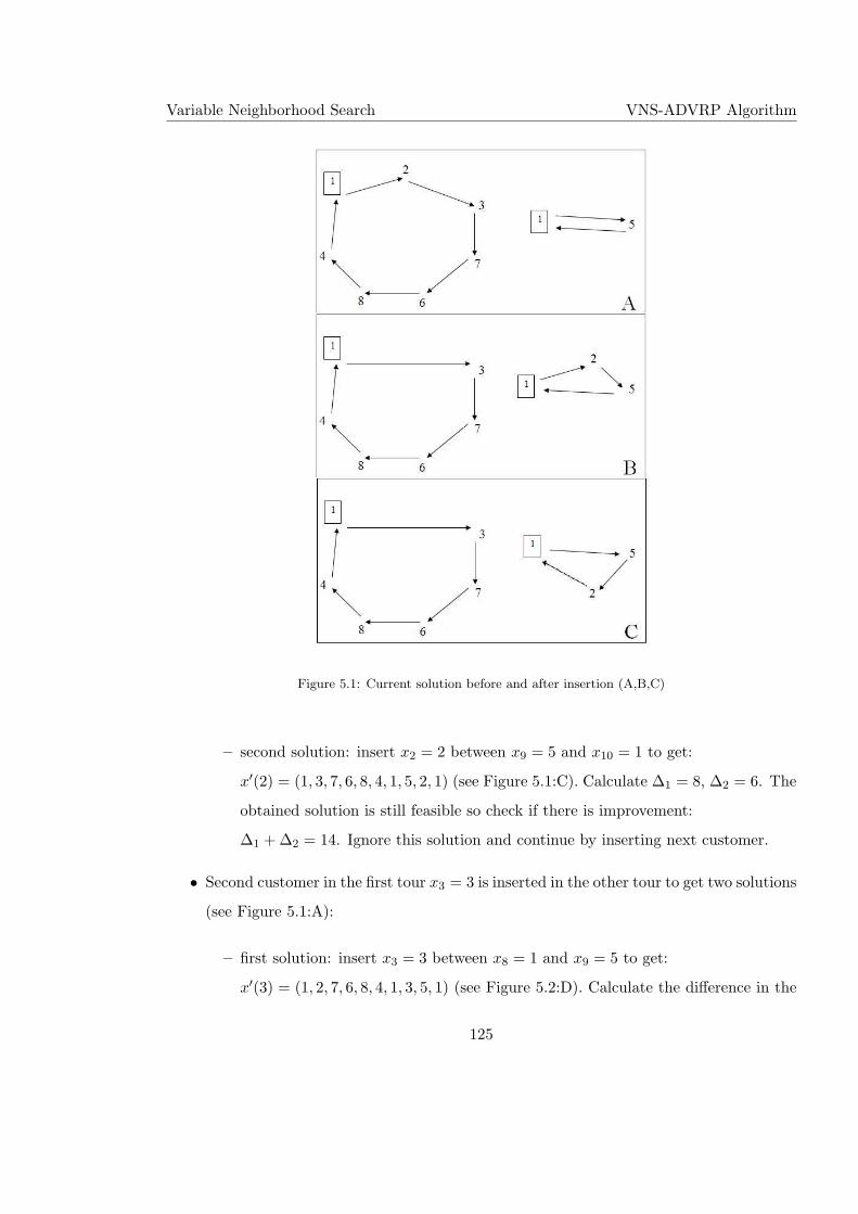
Variable Neighborhood Search VNS-ADVRP Algorithm
Figure 5.1: Current solution before and after insertion (A,B,C)
– second solution: insert x2 = 2 between x9 = 5 and x10 = 1 to get:
x′(2) = (1, 3, 7, 6, 8, 4, 1, 5, 2, 1) (see Figure 5.1:C). Calculate ∆1 = 8, ∆2 = 6. The
obtained solution is still feasible so check if there is improvement:
∆1 + ∆2 = 14. Ignore this solution and continue by inserting next customer.
• Second customer in the first tour x3 = 3 is inserted in the other tour to get two solutions
(see Figure 5.1:A):
– first solution: insert x3 = 3 between x8 = 1 and x9 = 5 to get:
x′(3) = (1, 2, 7, 6, 8, 4, 1, 3, 5, 1) (see Figure 5.2:D). Calculate the difference in the
125
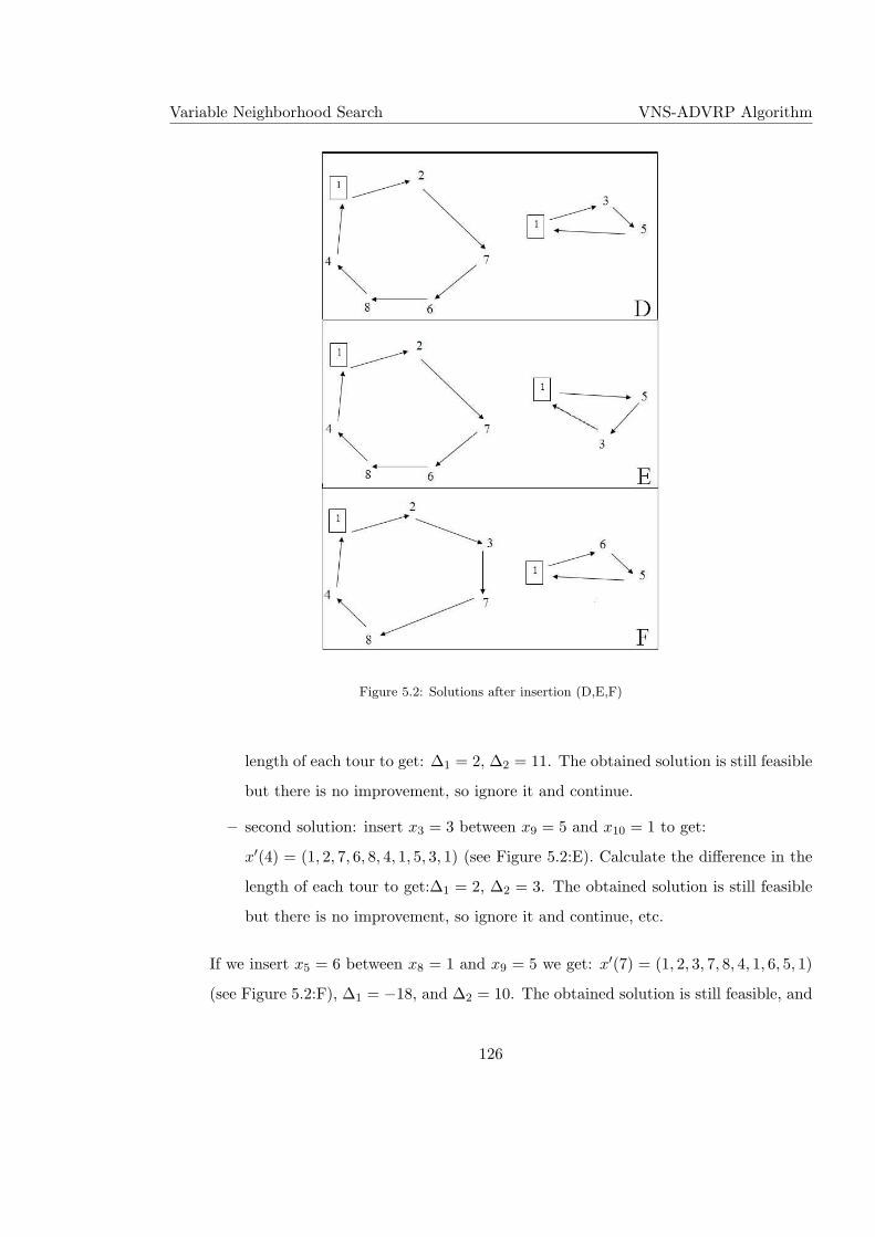
Variable Neighborhood Search VNS-ADVRP Algorithm
Figure 5.2: Solutions after insertion (D,E,F)
length of each tour to get: ∆1 = 2, ∆2 = 11. The obtained solution is still feasible
but there is no improvement, so ignore it and continue.
– second solution: insert x3 = 3 between x9 = 5 and x10 = 1 to get:
x′(4) = (1, 2, 7, 6, 8, 4, 1, 5, 3, 1) (see Figure 5.2:E). Calculate the difference in the
length of each tour to get:∆1 = 2, ∆2 = 3. The obtained solution is still feasible
but there is no improvement, so ignore it and continue, etc.
If we insert x5 = 6 between x8 = 1 and x9 = 5 we get: x′(7) = (1, 2, 3, 7, 8, 4, 1, 6, 5, 1)
(see Figure 5.2:F), ∆1 = −18, and ∆2 = 10. The obtained solution is still feasible, and
126
Variable Neighborhood Search Computational Results
there is an improvement since ∆1 + ∆2 = −8. So we save the solution, and update
x′′ = (1, 2, 3, 7, 8, 4, 1, 6, 5, 1), f(x′′) = f(x′) + ∆1 + ∆2 = 67 − 18 + 10 = 59. Set
x′ = x′′ = (1, 2, 3, 7, 8, 4, 1, 6, 5, 1) and start the local search again by inserting x2 = 2
between x7 = 1 and x8 = 6, and so on.
At the end of our VNS-ADVRP algorithm, we get x = (1, 2, 3, 1, 7, 8, 6, 4, 5, 1) as the best
feasible solution in 10 seconds, and the value of the objective function is f(x) = 34. Note
that the final solution obtained is optimal (see section 4.3.5).
5.3 Computational Results
All experiments were implemented under windows XP and on intel(R) Core(TM)2 CPU
[email protected], with 3.24 GB of RAM. The code is written in Fortran.
Test Instances. Full asymmetric distance matrices are generated at random using the uni-
form distribution to generate integer numbers. These integer numbers belong to one of these
intervals [1, 100], [1, 1000], [1, 10000]. The shortest distance between every two customers is
calculated. The size of test instances between 40 to 1000 customers is categorized as fol-
lows: small test instances {40, 80, .., 200}, large test instances {240, 280, .., 1000}. For each
n ≤ 200, two different number of vehicles are used: m1 = n/20 and m2 = n/10. For instances
240 ≤ n ≤ 1000, we use only m1.
We generate four different distance matrices for each combination of (n,m). However,
only one distance matrix is generated for large test instances (i.e., 200 < n ≤ 1000). The
maximum distance allowed is Dmax = ∞. The maximum CPU time for small test instances
is 10 seconds and for large test instances is 100 seconds. All test instances used in this thesis
can be found on the following web site: http://www.mi.sanu.ac.rs/∼nenad/advrp/
We evaluate the performance of VNS based on the difference between:
• the value of best feasible solution obtained by VNS.
• and the value of the optimal solution or the best value of feasible solution obtained so
far by the previous methods: MSBB-ADVRP, CPLEX-ADVRP.
127
Variable Neighborhood Search Conclusion
5.3.1 Data Structure
The initialization algorithm INIT-TSP requires the following information for each instance:
the number of vertices (n), the number of vehicles (m), maximum distance allowed (Dmax),
and the distance matrix (d).
The order of customers in the TSP solution is stored as xtsp = (x1, x2, ..., xn) while
the order in ADVRP is presented as: xdvrp = (x1, x2, ..., x1, xi, xi+1, ..., xn, x1) where x1
represents the depot and the others represent the customers. The total number that x1 will
appear in xdvrp is equal to (m + 1).
5.3.2 Numerical Analysis
We compared three methods: CPLEX-ADVRP, MSBB-ADVRP (see Chapter 4), and VNS-ADVRP.
The tables of results present the value of the objective function to the solution obtained
(optimal solution or best feasible solution found so far), CPU time, and %dev, where:
%dev =f(V NS)− f(bestknown)
f(bestknown)× 100 (5.2)
See Appendix B for more details about the results. The summary table contains the number
of vertices, the average %dev and the average CPU Time in each case (see Table 5.2).
The percentage of error (%dev) and the CPU Time increase when the number of cus-
tomers increase. The results we get are not good enough. In addition, when we reduced
Dmax, sometimes we faced difficulties in finding any feasible solution. The reason for this
is probably that the route-first-cluster-second approach is not suitable. In Appendix B, we
present some limited computational results for the case when Dmax is less than infinity.
We believe that the cluster-first-route-second approach will improve VNS results. How-
ever, when the number of customers increases, which may be a realistic urban problem, all
exact solution methods fail to reach a solution and a heuristic is the only choice.
128
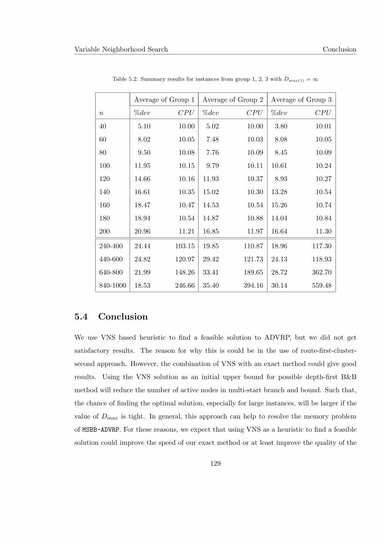
Variable Neighborhood Search Conclusion
Table 5.2: Summary results for instances from group 1, 2, 3 with Dmax(1) = ∞
Average of Group 1 Average of Group 2 Average of Group 3
n %dev CPU %dev CPU %dev CPU
40 5.10 10.00 5.02 10.00 3.80 10.01
60 8.02 10.05 7.48 10.03 8.08 10.05
80 9.50 10.08 7.76 10.09 8.45 10.09
100 11.95 10.15 9.79 10.11 10.61 10.24
120 14.66 10.16 11.93 10.37 8.93 10.27
140 16.61 10.35 15.02 10.30 13.28 10.54
160 18.47 10.47 14.53 10.54 15.26 10.74
180 18.94 10.54 14.87 10.88 14.04 10.84
200 20.96 11.21 16.85 11.97 16.64 11.30
240-400 24.44 103.15 19.85 110.87 18.96 117.30
440-600 24.82 120.97 29.42 121.73 24.13 118.93
640-800 21.99 148.26 33.41 189.65 28.72 362.70
840-1000 18.53 246.66 35.40 394.16 30.14 559.48
5.4 Conclusion
We use VNS based heuristic to find a feasible solution to ADVRP, but we did not get
satisfactory results. The reason for why this is could be in the use of route-first-cluster-
second approach. However, the combination of VNS with an exact method could give good
results. Using the VNS solution as an initial upper bound for possible depth-first B&B
method will reduce the number of active nodes in multi-start branch and bound. Such that,
the chance of finding the optimal solution, especially for large instances, will be larger if the
value of Dmax is tight. In general, this approach can help to resolve the memory problem
of MSBB-ADVRP. For these reasons, we expect that using VNS as a heuristic to find a feasible
solution could improve the speed of our exact method or at least improve the quality of the
129

Variable Neighborhood Search Conclusion
incumbent solution.
In future research, to improve VNS based heuristic for solving ADVRP, we suggest the
use of cluster-first-route-second approach and use of more neighborhood structures within
recent VNS methodologies see [95].
130
Chapter 6
Conclusions
6.1 Overview
In this thesis, exact and approximate solution methods for solving Asymmetric distance-
constrained vehicle routing problems (ADVRP) are discussed. In this chapter, we summarize
our scientific contributions, and also present future research directions. The main contribu-
tion of this thesis is the exact solution method for solving the larger instances compared to
previous work in the literature.
In Chapter 3, we presented a general flow based formulation for solving Asymmetric
distance- constraints vehicle routing problem (ADVRP). This formulation does not require the
distance matrix to satisfy the triangle inequality unlike Kara formulation (see [98]). It uses
the shortest distances between the depot and customers. This formulation is first illustrated
on an illustrative example. A computational comparison between this formulation and the
adapted formulation has been performed, showing advantages of our formulation.
In Chapter 4, we compared three methods for solving ADVRP: tolerance based branch-
ing (TOL-ADVRP), multistart branch and bound (MSBB-ADVRP), and commercial software
(CPLEX-ADVRP). TOL-ADVRP is a simple and fast method but has a memory consumption
problem. Therefore, we introduce the new method based on randomness in choosing the
next node in the branch and bound tree within multistart MSBB-ADVRP.
In Chapter 5, we tried to improve the initial upper bound of the exact method by using
131
Conclusions Future Research
variable neighborhood search (VNS). VNS uses the route-first-cluster-second approach. It
appears that it is not helpful to use VNS in providing the value of the upper bound for our
multistart method. The reason being that we use best first strategy which is able to find a
feasible solution in a short time.
6.2 Contribution
The goal of this research is to increase the size of ADVRP problems that can be solved exactly
in a reasonable CPU time. The thesis is divided into three main parts. The summary of
each part is given below:
• The first part presents a general formulation to ADVRP. It appears that our formulation
is more effective and efficient i.e., it shows good results in reducing the CPU time and
increasing the number of solved instances (see [9]).
• The second part proposes three methods to solve ADVRP. We showed that our multistart
method (MSBB-ADVRP) allowed us to solve larger instances than CPLEX does using the
formulation presented by Kara in [99]. The instances that we have solved exactly (up
to 1000 customers) are much larger than the instances considered for other VRPs from
the literature.
In addition, we achieve considerable reduction in the average running time. The per-
formance of CPLEX is worse for large instances while our method performs very well
on these instances. On the other hand, the reverse is satisfied for small instances (see
[11]).
• The third part uses VNS to find a good feasible solution to ADVRP in order to solve
very large problems or to improve the upper bound for the exact method. For large
instances, VNS is a better choice for finding a feasible solution in a short amount of
time than CPLEX, which sometimes is not able to find any feasible solution in 3 hours.
132
Conclusions Future Research
6.3 Future Research
• Our approach may be applied to other VRP variants, such as ADVRP with capacity
constraints, or in solving bus school routing problems.
• Instead of best first strategy, use guided dives search strategy (see [145] page 484).
• Combine the best-first-search with the depth-first-search: start with the best first
search then temporarily use depth first search as far as possible; next use the best first
search to jump to the best node in the search tree; then use the depth first search again
and so on.
• Improve the lower bound by using CPLEX to solve assignment constraints adding
2 new constraints (4.5 and 4.6). Use it as a procedure in exact method instead of
Hungarian algorithm.
• Another approach could be in using the lower tolerance-based branch-and-bound [60]
(instead of the upper tolerance used in this thesis).
133
Bibliography
[1] E. Aarts and J. K. Lenstra. Local search in combinatorial optimization. John Wiley & Sons
Ltd, 1997.
[2] E. H. L. Aarts, J. H. M. Korst, and P. J. M. van Laarhoven. Simulated annealing. In: E. Aarts
and J. K. Lenstra, eds., Local search in combinatorial optimization, chapter 4, pages 91–120.
John Wiley & Sons Ltd, 1997.
[3] T. Achterberg, T. Koch, and A. Martin. Branching rules revisited. Operations Research Letters,
33:42–54, 2005.
[4] M. Affenzeller, S. Winkler, S. Wagner, and A. Beham. Genetic algorithms and genetic pro-
gramming: modern concepts and practical applications. CRC Press, 2009.
[5] A. S. Alfa, S. S. Heragu, and M. Chen. A 3-opt based simulated annealing algorithm for vehicle
routing problems. Computers & Industrial Engineering, 21:635–639, 1991.
[6] S. Almoustafa. Optimal solution to distance–constrained vehicle routing problems based on
tolerances. Master Dissertation, Manchester University, 2007.
[7] S. Almoustafa, B. Goldengorin, M. Tso, and N. Mladenovic. Two new exact methods for
asymmetric distance-constrained vehicle routing problem. Proceedings of SYM-OP-IS, pages
297–300, 2009.
[8] S. Almoustafa, S. Hanafi, and N. Mladenovic. Multistart approach for exact vehicle routing.
Proceedings of Balcor, pages 162–170, 2011.
[9] S. Almoustafa, S. Hanafi, and N. Mladenovic. New formulation for the distance-constrained
vehicle routing problem. Proceedings of SYM-OP-IS, pages 383–387, 2011.
[10] S. Almoustafa, S. Hanafi, and N. Mladenovic. Multistart branch and bound for large asymmet-
ric distance-constrained vehicle routing problem. In: A. Migdalas and A. Sifaleras and C.K.
134
Bibliography
Georgiadis and J. Papathanasiou and E. Stiakakis (eds.), Optimization Theory, Decision Mak-
ing, and Operational Research Applications., chapter 2, pages 15–38. Springer Proceedings in
Mathematics & Statistics 31, 2012.
[11] S. Almoustafa, S. Hanafi, and N. Mladenovic. New exact method for large asymmetric distance-
constrained vehicle routing problem. European Journal of Operational Research, 226(3):386–
394, 2013.
[12] F. Alonso, M. J. Alvarez, and J. E. Beasley. A tabu search algorithm for the periodic vehi-
cle routing problem with multiple vehicle trips and accessibility restrictions. Journal of the
Operational Research Society, 59:963–976, 2008.
[13] E. Balas and P. Toth. Branch and bound method. In: E.L. Lawer and J.K. Lenstra and A.
H. G. Rinnooy Kan and D.B. Shmoys, eds., The traveling salesman problem: a guided tour of
combinatorial optimization, chapter 10, pages 361–401. Chichester : Wiley, 1985.
[14] R. Baldacci, E. Hadjiconstantinou, and A. Mingozzi. An exact algorithm for the capacitated
vehicle routing problem based on a two-commodity network flow formulation. Operations Re-
search, 52(5):723–738, 2004.
[15] R. Baldacci and A. Mingozzi. An unified exact method for solving different classes of vehicle
routing problems. Mathematical Programming Ser. A, 120(2):347–380, 2009.
[16] R. Baldacci, A. Mingozzi, and R. Roberti. Recent exact algorithms for solving the vehicle
routing problem under capacity and time window constraints (invited review). European Journal
of Operational Research, 218(1):1–6, 2012.
[17] R. Baldacci, P. Toth, and D. Vigo. Recent advances in vehicle routing exact algorithms. 4OR,
5(4):269–298, 2007.
[18] M. Balinski and R. Quandt. On an integer program for a delivery problem. Operations Research,
12:300–304, 1964.
[19] J. E. Beasley. Route-first cluster-second methods for vehicle routing. Omega, 11:403–408, 1983.
[20] T. Bektas and S. Elmastas. Solving school bus routing problems through integer programming.
Journal of Operational Research Society, 58:1599–1604, 2007.
[21] J. E. Bell and P. R. Mcmullen. Ant colony optimization techniques for the vehicle routing
problem. Advanced Engineering Informatics, 18:41–48, 2004.
135
Bibliography
[22] R. Bellman. The theory of dynamic programming. Bull. Amer. Math. Soc., 60:503–515, 1954.
[23] A. M. Benjamin and J. E. Beasley. Metaheuristics for the waste collection vehicle routing
problem with time windows, driver rest period and multiple disposal facilities. Computers &
Operations Research, 37(12):2270–2280, 2010.
[24] C. Blum, C. Cotta, A. J. Fernandez, J. E. Gallardo, and M. Mastrolilli. Hybridizations of
metaheuristics with branch & bound derivates. In: C. Blum and M. J. B. Aguilera and A. Roli
and M. Sampels, eds., Hybrid metaheuristics an emerging approach to optimization, chapter 4,
pages 85–116. Springer, 2008.
[25] C. Blum and A. Roli. Hybrid metaheuristics: an introduction. In: C. Blum and M. J. B.
Aguilera and A. Roli and M. Sampels, eds., Hybrid metaheuristics an emerging approach to
optimization, chapter 1, pages 1–30. Springer, 2008.
[26] J. Bramel and D. Simchi-Levi. Set-covering-based algorithms for the capacitated VRP. In: P.
Toth and D. Vigo, eds., The vehicle routing problem, chapter 4, pages 85–108. SIAM, 2002.
[27] J. Brimberg, N. Mladenovic, D. Urosevic, and E. Ngai. Variable neighborhood search for the
heaviest k-subgraph. Computers & Operations Research, 36(11):2885–2891, 2009.
[28] G. Carpaneto and P. Toth. Some new branching and bounding criteria for the asymmetric
traveling salesman problem. Management Science, 26:736–743, 1980.
[29] A. Chabrier. Vehicle routing problem with elementary shortest path based column generation.
Computers & Operations Research, 33:2972–2990, 2006.
[30] L. Chambers. Practical handbook of genetic algorithms. CRC Press, Inc, 1995.
[31] N. Christofides, A. Mingozzi, and P. Toth. State space relaxation procedures for the computa-
tion of bounds to routing problems. Networks, 11(2):145–164, 1981.
[32] G. Clarke and J. W. Wright. Scheduling of vehicles from a central depot to a number of delivery
points. Operations Research, 12(4):568–581, 1964.
[33] S. Climer and W. Zhang. Cut and solve: an iterative search strategy for combinatorial opti-
mization problems. Artificial Intelligence, 170:714–738, 2006.
[34] J. F. Cordeau, G. Desaulniers, J. Desrosiers, M. M. Solomon, and F. Soumis. VRP with time
windows. In: P. Toth and D. Vigo, eds., Vehicle routing problem, chapter 7, pages 157–194.
SIAM, 2002.
136
Bibliography
[35] J. F. Cordeau, M. Gendreau, G. Laporte, J. Y. Potvin, and F. Semet. A guide to vehicle routing
heuristics. Journal of the Operational Research Society, 53:512–522, 2002.
[36] J. F. Cordeau and G. Laporte. Modeling and optimization of vehicle routing problem. In: G.
Appa, L. Pitsoulis, H. P. Williams. eds., Handbook on modelling for discrete optimization,
chapter 6, pages 151–194. New York: Springer, 2006.
[37] M. C. Costa, F. R. Monclar, and M. Zrikem. Variable neighborhood decomposition search for
the optimization of power plant cable layout. Journal of Intelligent Manufacturing, 13(5):353–
365, 2002.
[38] T. G. Crainic and G. Laporte. Fleet management and logistics. Boston, Mass; London: Kluwer,
1998.
[39] G. B. Dantzig, D. R. Fulkerson, and S. M. Johnson. Solution of a large-scale traveling salesman
problem. Journal of the Operations Research Society of America, 2(4):393–410, 1954.
[40] G. B. Dantzig and J. H. Ramser. The truck dispatching problem. Management Science, 6(1):80–
91, 1959.
[41] L. Davis. Handbook of genetic algorithms. New York: Van Nostrand Reinhold, 1991.
[42] E. Demir and I. Kara, 2008. Formulations for school bus routing problems, 21st conference on
combinatorial optimization, Dubrovnik, Croatia, May 29-31.
[43] G. Desaulniers, J. Desrosiers, A. Erdmann, M. M. Solomon, and F. Soumis. VRP with pickup
and delivery. In: P.Toth and D. Vigo, eds., Vehicle routing problem, chapter 9, pages 225–242.
SIAM, 2002.
[44] G. Desaulniers, J. Desrosiers, and M. M. Solomon. Column generation. Gerad 25th Anniversary
Series. Springer, 2005.
[45] M. Dorigo and T. Stutzle. Ant colony optimization. MIT, 2004.
[46] M. Dorigo and T. Stutzle. Ant colony optimization: overview and recent advances. In: M. Gne-
dreau and J. Y. Potvin, eds., Handbook of metaheuristics, chapter 8, pages 227–264. Springer,
2010.
[47] K. A. Dowsland. Classical techniques. In: E. K. Burke and G. Kendall, eds., Search method-
ologies Introductory tutorials in optimization and decision support techniques, chapter 2, pages
19–68. Springer, 2005.
137
Bibliography
[48] M. Drexl. Rich vehicle routing in theory and practice. Logistics Research, 5:47–63, 2012.
[49] M. Fisher. Vehicle routing. In: M.O. Ball and T.L. Magnanti and C.L. Monma and G.L.
Nemhauser. Network routing, Handbooks in operations research and management science, vol
8, chapter 1, pages 1–33. North-Holland: Amsterdam, 1995.
[50] M. L. Fisher and R. Jaikumar. A generalized assignment heuristic for vehicle routing. Networks,
11(2):109–124, 1981.
[51] R. Fukasawa, H. Longo, J. Lysgaard, M. Poggi de Aragao, M. Reis, E. Uchoa, and R. F.
Werneck. Robust branch-and-cut-and-price for the capacitated vehicle routing problem. Math-
ematical Programming Series A, 106(3):491–511, 2006.
[52] W. W. Garvin, H. W. Crandall, J. B. John, and R. A. Spellman. Applications of vehicle routing
in the oil industry. Management Science, 3:407–430, 1957.
[53] M. Gendreau. An Introduction to tabu search. In: F. Glover and G. A. Kochenberger, eds.,
Handbook of metaheuristics, chapter 2, pages 37–54. Kluwer Academic Publishers, 2003.
[54] M. Gendreau, A. Hertz, and G. Laporte. A tabu search heuristic for the vehicle routing problem.
Management Science, 40(10):1276–1290, 1994.
[55] M. Gendreau, G. Laporte, and J. Y. Potvin. Vehicle routing: modern heuristics. In: E. Aarts
and J. K. Lenstra, eds., Local search in combinatorial optimization, chapter 9, pages 311–336.
John Wiley & Sons Ltd, 1997.
[56] M. Gendreau, G. Laporte, and J. Y. Potvin. Metaheuristics for the capacitated VRP. In: P.
Toth and D. Vigo, eds., Vehicle routing problem, chapter 6, pages 129–154. SIAM, 2002.
[57] M. Gendreau and J. Y. Potvin. Metaheuristics in combinatorial optimization. Annals of Oper-
ations Research, 140:189–213, 2005.
[58] M. Gendreau and J. Y. Potvin. Handbook of metaheuristics. Springer, 2010.
[59] M. Gendreau and J. Y. Potvin. Tabu search. In: M. Gnedreau and J. Y. Potvin, eds., Handbook
of metaheuristics, chapter 2, pages 41–59. Springer, 2010.
[60] R. Germs, B. Goldengorin, and M. Turkensteen. Lower tolerance-based branch and bound
algorithms for the atsp. Computers & Operations Research, 39:291–298, 2012.
[61] B. E. Gillett and L. R. Miller. A heuristic algorithm for the vehicle-dispatch problem. Operations
Research, 22(2):340–349, 1974.
138
Bibliography
[62] F. Glover. Future paths for integer programming and links to artificial intelligence. Computers
and Operations Research, 13(5):533–549, 1986.
[63] F. Glover and G.A. Kochenberger. Handbook of metaheuristics. Kluwer Academic Publishers,
2003.
[64] F. Glover and M. Laguna. Tabu search. Boston; London: Kluwer, 1997.
[65] F. Glover, M. Laguna, and R. Marti. Scatter search and path relinking: advances and appli-
cations. In: F. Glover and G.A. Kochenberger, eds., Handbook of metaheuristics, chapter 1,
pages 1–36. Kluer, 2003.
[66] A. Goel and V. Gruhn. A general vehicle routing problem. European Journal of Operational
Research, 191:650–660, 2008.
[67] D. E. Goldberg. Genetic algorithms in search, optimization and machine learning. Reading,
MA: Addison-Wesley, 1989.
[68] B. Golden, S. Raghavan, and E. Wasil. The vehicle routing problem: latest advances and new
challenges. Springer, 2008.
[69] B. L. Golden and A. A. Assad. Vehicle routing: methods and studies. North-Holland, 1988.
[70] B. Goldengorin. Synergy effects in branch-and-bound algorithms for the asymmetric capacitated
vehicle routing problem. Technical report, 2006.
[71] B. Goldengorin. Tolerance-based bnb algorithm for the asymmetric distance-capacitated vehicle
routing problem: a numerical example. Personal Communication, 2006.
[72] B. Goldengorin, G. Jager, and P. Molitor. Tolerances applied in combinatorial optimization.
Journal of Computer Science, 2(9):716–734, 2006.
[73] R. E. Gomory. Outline of an algorithm for integer solutions to linear programs. Bulletin of the
American Mathematical Society, 64:275–278, 1958.
[74] J. Gondzio, P. Gonzlez-Brevis, and P. Munari. New developments in the primal-dual column
generation technique. European Journal of Operational Research, 224(1):41–51, 2013.
[75] M. Haimovich, A. H. G. Rinnooy Kan, and L. Stougie. Analysis of heuristic routing problems.
In: B. L. Golden and A. A. Assad, eds., Vehicle routing: methods and studies, chapter 6, pages
47–61. North-Holland, 1988.
139
Bibliography
[76] P. Hansen, J. Lazic, and N. Mladenovic. Variable neighbourhood search for colour image
quantization. IMA Journal of Management Mathematics, 18(2):207–221, 2007.
[77] P. Hansen and N. Mladenovic. An introduction to variable neighborhood search. In: S. Voss
and S. Martello and I. H. Osman and C. Roucairol, eds., Metaheuristics: advances and trends
in local search paradigms for optimization, chapter 30, pages 433–458. Kluwer, 1999.
[78] P. Hansen and N. Mladenovic. Developments of Variable Neighborhood Search. In: C.C. Ribeiro
and P. Hansen, eds., Essays and Surveys in Metaheuristics, chapter 19, pages 415–440. Oxford
University Press, 2000.
[79] P. Hansen and N. Mladenovic. Variable neighbourhood search: principles and applications.
European Journal of Operational Research, 130(3):449–467, 2001.
[80] P. Hansen and N. Mladenovic. Variable neighborhood search. In: P.M. Pardalos and M.G.C.
Resende, eds., Handbook of Applied Optimization, pages 221–234. Oxford University Press,
2002.
[81] P. Hansen and N. Mladenovic. Variable neighborhood search. In: F. Glover and G.A. Kochen-
berger, eds., Handbook of metaheuristics, chapter 6, pages 145–184. Kluer, 2003.
[82] P. Hansen and N. Mladenovic. First vs. best improvement: an empirical study. Discrete Applied
Mathematics, 154:802–817, 2006.
[83] P. Hansen, N. Mladenovic, J. Brimberg, and J. A. Moreno. Variable neighbourhood search.
In: M. Gnedreau and J. Y. Potvin, eds., Handbook of metaheuristics, chapter 3, pages 61–86.
Springer, 2010.
[84] P. Hansen, N. Mladenovic, and J.A. Moreno Perez. Variable neighbourhood search: methods
and applications. 4OR: Quarterly Journal of Operations Research, 6(4):319–360, 2008.
[85] P. Hansen, N. Mladenovic, and J.A. Moreno Perez. Variable neighbourhood search: methods
and applications. Annals of Operations Research, 175(1):367–407, 2010.
[86] P. Hansen, N. Mladenovic, and D. Perez-Britos. Variable neighborhood decomposition search.
Journal of Heuristics, 7(4):335–350, 2001.
[87] P. Hansen, N. Mladenovic, and D. Urosevic. Variable neighborhood search and local branching.
Computers and Operations Research, 33(10):3034–3045, 2006.
140
Bibliography
[88] A. Hertz, E. Taillard, and D. de Werra. Tabu search. In: E. Aarts and J. K. Lenstra, eds.,
Local search in combinatorial optimization, chapter 5, pages 121–136. John Wiley & Sons Ltd,
1997.
[89] F. S. Hillier and G. J. Lieberman. Introduction to operations research. McGraw-Hill, 2010.
[90] K. L. Hoffman and M. Padberg. Improving lp-representations of zero=one linear programs for
branch and cut. ORSA Journal on Computing, 3:121–134, 1991.
[91] J. H. Holland. Adaptation in natural and artificial systems. The University of Michigan Press,
Ann Arbor, MI, 1975.
[92] J. H. Holland. Adaptation in natural and artificial systems. MIT Press, 1992.
[93] A. Ilic, D. Urosevic, J. Brimberg, and N. Mladenovic. A general variable neighborhood search
for solving the uncapacitated single allocation p-hub median problem. European Journal of
Operational Research, 206:289–300, 2010.
[94] A. Imran, S. Salhi, and N. A. Wassan. A variable neighborhood-based heuristic for the hetero-
geneous fleet vehicle routing problem. European Journal of Operational Research, 197:509–518,
2009.
[95] B. Jarboui, H. Derbel, S. Hanafi, and N. Mladenovic. Variable neighborhood search for location
routing. Computers & Operations Research, 40:47–57, 2013.
[96] D. S. Johnson and C. H. Papadimitriou. Computational complexity. In: E.L. Lawer and J.K.
Lenstra and A. H. G. Rinnooy Kan and D.B. Shmoys, eds., The traveling salesman problem: a
guided tour of combinatorial optimization, chapter 3, pages 37–86. Chichester: Wiley, 1985.
[97] R. Jonker and A. Volgenant. Improving the hungarian assignment algorithm. Operations
Research Letters, 5(4):171–175, 1986.
[98] I. Kara. Arc based integer programming formulations for the distance constrained vehicle
routing problem. In 3rd IEEE International Symposium on Logistics and Industrial informatics,
pages 33–38, 2011.
[99] I. Kara. Two indexed polynomial size formulations for vehicle routing problems. Technical
report, June 2008.
[100] I. Kara and T. Derya. Polynomial size formulations for the distance and capacity constrained
vehicle routing problem. In AIP conf. Proc. 1389; doi:10.1063/1.3636940, pages 1713–1718,
2011.
141
Bibliography
[101] I. Kara, B. Y. Kara, and M.K. Yetis. Energy minimizing vehicle routing problem. In: A. Dress
and Y. Xu and B. Zhu, eds., Combinatorial optimization and applications, pages 62–71. LNCS
4616, Springer, Berlin, Heidelberg, 2007.
[102] G. A. P. Kindervater and M. W. P. Savelsbergh. Vehicle routing problem: handling edge
exchanges. In: E. Aarts and J. K. Lenstra, eds., Local search in combinatorial optimization,
chapter 10, pages 337–360. John Wiley & Sons Ltd, 1997.
[103] T. Koltai and T. Terlaky. The difference between the managerial and mathematical interpreta-
tion of sensitivity analysis results in linear programming. International Journal of Production
Economics, 65(3):257–274, 2000.
[104] H. W. Kuhn. The hungarian method for the assignment problem. Naval Research Logistics
Quarterly, 2:83–97, 1955.
[105] P.J. Van Laarhoven and E. H. Aarts. Simulated annealing: theory and applications. Kluwer,
1987.
[106] G. Laporte. The vehicle routing problem: an overview of exact and approximate algorithms.
European Journal of Operational Research, 59(3):345–358, 1992.
[107] G. Laporte. Fifty years of vehicle routing. Transportation Science, 43(4):408–416, 2009.
[108] G. Laporte and M. Desrochers. Two exact algorithms for the distance-constrained vehicle
routing problem. Networks, 14:161–172, 1984.
[109] G. Laporte, M. Gendreau, J. Y. Potvin, and F. Semet. Classical and modern heuristics for the
vehicle routing problem. International Transactions in Operational Research, 7:285–300, 2000.
[110] G. Laporte, H. Mercure, and Y. Nobert. An exact algorithm for the asymmetrical capacitated
vehicle routing problem. Networks, 16:33–46, 1986.
[111] G. Laporte and Y. Nobert. Exact algorithms for the vehicle routing problem. Annals of Discrete
Mathematics, 31:147–184, 1987.
[112] G. Laporte, Y. Nobert, and M. Desrochers. Optimal routing under capacity and distance
restrictions. Operations Research, 33(5):1050–1073, 1985.
[113] G. Laporte, Y. Nobert, and S. Taillefer. A branch and bound algorithm for the asymmetrical
distance-constrained vehicle routing problem. Mathematical Modelling, 9(12):875–868, 1987.
142
Bibliography
[114] G. Laporte and I. H. Osman. Routing problems: a bibliography. Annals of Operations Research,
61:227–262, 1995.
[115] G. Laporte and F. Semet. Classical heuristics for the capacitated VRP. In: P. Toth and D.
Vigo, eds., Vehicle routing problem, chapter 5, pages 109–128. SIAM, 2002.
[116] E. L. Lawer, J. K. Lenstra, A. H. G. Rinnooy Kan, and D. B. Shmoys. The traveling salesman
problem: a guided tour of combinatorial optimization. Wiley, 1985.
[117] J. Lazic, S. Hanafi, N. Mladenovic, and D. Urosevic. Variable neighbourhood decomposition
search for 0-1 mixed integer programs. Computers & Operations Research, 37(6):1055–1067,
2010.
[118] M. E. Lubbecke. Column generation. Springer, 2010.
[119] M. A. Lejeune. A variable neighborhood decomposition search method for supply chain man-
agement planning problems. European Journal of Operational Research, 175(2):959–976, 2006.
[120] J. K. Lenstra and A. H. G. Rinnooy Kan. Some simple applications of the travelling salesman
problem. Operational Research Quarterly, 26(4):717–733, 1975.
[121] A. N. Letchford and J. J. Salazar-Gonzalez. Projection results for vehicle routing. Mathematical
Programming, Ser. B, 105:251–274, 2006.
[122] C. L. Li, D. Simchi-Levi, and M. Desrochers. On the distance constrained vehicle routing
problem. Operations Research, 40(4):790–799, 1992.
[123] C. Lin and U. Wen. Sensitivity analysis of the optimal assignment. Discrete Optimization,
149(1):35–46, 2003.
[124] J. T. Linderoth and M. W. P. Savelsbergh. A computational study of search strategies for
mixed integer programming. INFORMS Journal on Computing, 11(2):137–187, 1999.
[125] R. Martı. Multi-start methods. In: F. Glover and G.A. Kochenberger, eds., Handbook of meta-
heuristics, chapter 12, pages 355–368. Kluer, 2003.
[126] R. Martı, J. M. Moreno-Vega, and A. Duarte. Advanced multi-start methods. In: M. Gnedreau
and J. Y. Potvin, eds., Handbook of metaheuristics, chapter 9, pages 265–282. Springer, 2010.
[127] Z. Michalewicz. Genetic algorithms + data structures = evolution programs. Springer, Berlin,
1996.
[128] Z. Michalewicz and D. B. Fogel. How to solve it: modern heuristics. Springer, 2004.
143
Bibliography
[129] J. E. Mitchell. Branch and cut. Wiley encyclopedia of operations research and management
science. John Wiley & Sons, Inc, 2010.
[130] N. Mladenovic, M. Drazic, V. Kovacevic-Vujcic, and M. Cangalovic. General variable neigh-
bourhood search for the continuous optimization. European Journal of Operational Research,
191(3):753–770, 2008.
[131] N. Mladenovic and P. Hansen. Variable neighbourhood search. Computers and Operations
Research, 24(11):1097–1100, 1997.
[132] N. Mladenovic, N. Labbe, and P. Hansen. Solving the p-center problem by tabu search and
variable neighbourhood search. Networks, 42:48–64, 2003.
[133] N. Mladenovic, J. Petrovic, V. Kovacevic-Vujcic, and M. Cangalovic. Solving spread spec-
trum radar polyphase code design problem by tabu search and variable neighbourhood search.
European Journal of Operational Research, 151:389–399, 2003.
[134] N. Mladenovic and D. Urosevic. Variable neighbourhood search for the k-cardinality tree.
Applied Optimization, 86:481–500, 2003.
[135] N. Mladenovic, D. Urosevic, S. Hanafi, and A. Ilic. A general variable neighborhood search
for the one-commodity pickup-and-delivery travelling salesman problem. European Journal of
Operational Research, 220(1):270–285, 2012.
[136] H. Muhlenbein. Genetic algorithms. In: E. Aarts and J. K. Lenstra, eds., Local search in
combinatorial optimization, chapter 6, pages 137–172. John Wiley & Sons Ltd, 1997.
[137] D. Naddef and G. Rinaldi. Branch and cut algorithms for the capacitated VRP. In: P. Toth
and D. Vigo, eds., Vehicle routing problem, chapter 3, pages 53–84. SIAM, 2002.
[138] A. G. Nikolaev and S. H. Jacobson. Simulated annealing. In: M. Gnedreau and J. Y. Potvin,
eds., Handbook of metaheuristics, chapter 1, pages 1–40. Springer, 2010.
[139] I. H. Osman. Metastrategy simulated annealing and tabu search algorithms for the vehicle
routing problem. Annals of Operations Research, 41(4):421–451, 1993.
[140] I. H. Osman and J. P. Kelly. Meta-heuristics: An overview. In: I. H. Osman and J. P. Kelly,
eds., Meta-heuristics: theory & applications, chapter 1, pages 1–22. Kluwer, 1996.
[141] V. Th. Paschos. An overview on polynomial approximation of np-hard problems. Yugoslav
Journal of Operations Research, 19(1):3–40, 2009.
144
Bibliography
[142] A. Pessoa, M. Poggi de Aragao, and E. Uchoa. Robust branch-cut-and-price algorithms for
vehicle routing problems. In: B. Golden and S. Raghavan and E. Wasil , eds., The vehicle
routing problem latest advances and new challenges, pages 297–325. Springer, 2008.
[143] C. Peterson and B. Soderberg. Artificial neural networks. In: E. Aarts and J. K. Lenstra, eds.,
Local search in combinatorial optimization, chapter 7, pages 173–214. John Wiley & Sons Ltd,
1997.
[144] G. R. Raidl and J. Puchinger. Combining (integer) linear programming techniques and meta-
heuristics for combinatorial optimization. In: C. Blum and M. J. B. Aguilera and A. Roli and
M. Sampels, eds., Hybrid metaheuristics an emerging approach to optimization, chapter 2, pages
31–62. Springer, 2008.
[145] G. R. Raidl, J. Puchinger, and C. Blum. Metaheuristics hybrids. In: M. Gendreau and J. Y.
Potvin, eds., Handbook of metaheuristics, chapter 16, pages 469–496. Springer, 2010.
[146] C. R. Reeves. Modern heuristic techniques for combinatorial problems. John Wiley & Sons,
Inc, 1993.
[147] C. R. Reeves. Genetic algorithms. In: M. Gnedreau and J. Y. Potvin, eds., Handbook of
metaheuristics, chapter 5, pages 109–140. Springer, 2010.
[148] C. R. Reeves and J. E. Rowe. Genetic algorithms - Principles and perspectives. Kluwer, Norwell,
MA, 2002.
[149] S. Remde, P. Cowling, K. Dahal, and N. Colledge. Exact/heuristic hybrids using rvns and
hyperheuristics for workforce scheduling. In EvoCOP’07 Proceedings of the 7th European con-
ference on Evolutionary computation in combinatorial optimization, pages 188–197, 2007.
[150] M. G. C. Resende and C. C. Riberio. Greedy randomized adaptive search procedures. In: F.
Glover and G.A. Kochenberger, eds., Handbook of metaheuristics, chapter 8, pages 219–249.
Kluer, 2003.
[151] M. G. C. Resende and C. C. Riberio. Greedy randomized adaptive search procedures: advances,
hybridizations, and application. In: M. Gnedreau and J. Y. Potvin, eds., Handbook of meta-
heuristics, chapter 10, pages 283–320. Springer, 2010.
[152] M. G. C. Resende, C. C. Riberio, f. Glover, and R. Martı. Scatter search and path-relinking:
fundamentals, advances, and applications. In: M. Gnedreau and J. Y. Potvin, eds., Handbook
of metaheuristics, chapter 4, pages 87–108. Springer, 2010.
145
Bibliography
[153] S. Salhi and R. Petch. A ga based heuristic for the vehicle routing problem with multiple trips.
Journal of Mathematical Modelling and Algorithms, 6(4):591–613, 2007.
[154] Scvalex. All sources shortest path: The floyd-warshall algorithm.
http://compprog.wordpress.com/2007/11/15/all-sources-shortest-path-the-floyd-warshall-
algorithm, 2007.
[155] J. Silberholz and B. Golden. Comparison of metaheuristics. In: M. Gnedreau and J. Y. Potvin,
eds., Handbook of metaheuristics, chapter 21, pages 625–640. Springer, 2010.
[156] M.C. De Souza and P. Martins. Skewed vns enclosing second order algorithm for the de-
gree constrained minimum spanning tree problem. European Journal of Operational Research,
191(3):677–690, 2008.
[157] P. Toth and D. Vigo . Branch and bound algorithms for the capacitated VRP. In: P. Toth and
D. Vigo, eds., Vehicle routing problem, chapter 2, pages 29–52. SIAM, 2002.
[158] P. Toth and D. Vigo . An overview of vehicle routing problems. In: P. Toth and D. Vigo, eds.,
Vehicle routing problem, chapter 1, pages 1–26. SIAM, 2002.
[159] P. Toth and D. Vigo . VRP with backhauls. In: P. Toth and D. Vigo, eds., Vehicle routing
problem, chapter 8, pages 195–224. SIAM, 2002.
[160] P. Toth and D. Vigo. The vehicle routing problem. SIAM, 2002.
[161] M. Turkensteen, D. Ghosh, B. Goldengorin, and G. Sierksma. Tolerance-based branch and
bound algorithms for the atsp. European Journal of Operational Research, 189(3):775–788,
2008.
[162] L. Vogt, C. A. Poojari, and J. E. Beasley. A tabu search algorithm for the single vehicle routing
allocation problem. Journal of the Operational Research Society, 58:467–480, 2007.
[163] A. Volgenant. An addendum on sensitivity analysis of the optimal assignment. European
Journal of Operational Research, 169(1):338–339, 2006.
[164] C. Voudouris, E. P. K. Tsang, and A. Alsheddy. Guided local search. In: M. Gnedreau and J.
Y. Potvin, eds., Handbook of metaheuristics, chapter 11, pages 321–362. Springer, 2010.
[165] C. D. J. Waters. Expanding the scope of linear programming solutions for vehicle scheduling
problems. Omega, 16(6):577–583, 1988.
146
Bibliography
[166] H. P. Williams. The formulation and solution of discrete optimization models. In: G. Appa,
L. Pitsoulis, H. P. Williams. eds., Handbook on modelling for discrete optimization, chapter 1,
pages 3–60. New York: Springer, 2006.
[167] D. L. Woodruff. A chunking based selection strategy for integrating metaheuristics with branch
and bound. In: S. Voss and S. Martello and I. H. Osman and C. Roucairol, eds., Metaheuristics:
advances and trends in local search paradigms for optimization, chapter 34, pages 499–511.
Kluwer, 1999.
[168] M. Yannakakis. Computational complexity. In: E. Aarts and J. K. Lenstra, eds., Local search
in combinatorial optimization, chapter 2, pages 19–56. John Wiley & Sons Ltd, 1997.
[169] L. C. Yeun, W. R. Ismail, K. Omar, and M. Zirour. Vehicle routing problem: models and
solutions. Journal of Quality Measurement and Analysis, 4(1):205–218, 2008.
[170] R. Zhou and E. A. Hansen. Breadth-first heuristic search. Artificial Intelligence, 170:385–408,
2006.
147
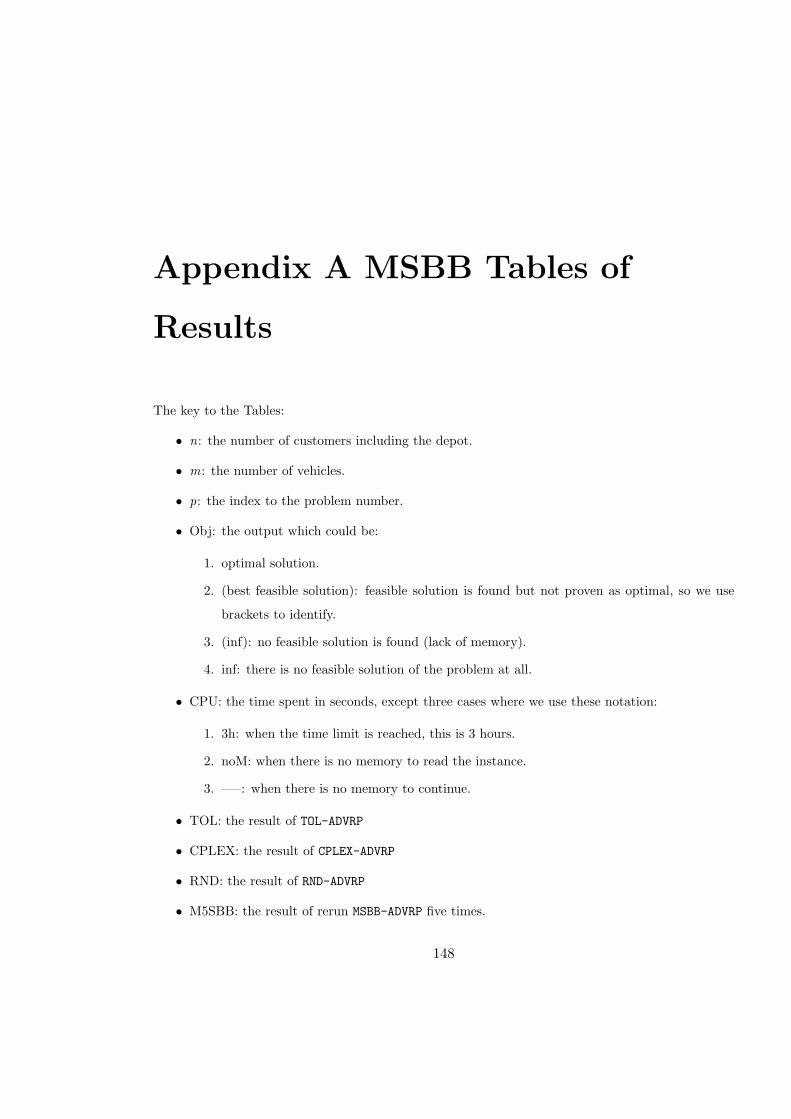
Appendix A MSBB Tables of
Results
The key to the Tables:
• n: the number of customers including the depot.
• m: the number of vehicles.
• p: the index to the problem number.
• Obj: the output which could be:
1. optimal solution.
2. (best feasible solution): feasible solution is found but not proven as optimal, so we use
brackets to identify.
3. (inf): no feasible solution is found (lack of memory).
4. inf: there is no feasible solution of the problem at all.
• CPU: the time spent in seconds, except three cases where we use these notation:
1. 3h: when the time limit is reached, this is 3 hours.
2. noM: when there is no memory to read the instance.
3. —–: when there is no memory to continue.
• TOL: the result of TOL-ADVRP
• CPLEX: the result of CPLEX-ADVRP
• RND: the result of RND-ADVRP
• M5SBB: the result of rerun MSBB-ADVRP five times.
148
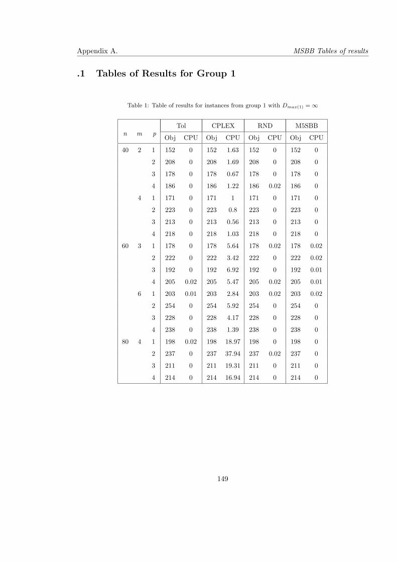
Appendix A. MSBB Tables of results
.1 Tables of Results for Group 1
Table 1: Table of results for instances from group 1 with Dmax(1) = ∞
Tol CPLEX RND M5SBBn m p
Obj CPU Obj CPU Obj CPU Obj CPU
40 2 1 152 0 152 1.63 152 0 152 0
2 208 0 208 1.69 208 0 208 0
3 178 0 178 0.67 178 0 178 0
4 186 0 186 1.22 186 0.02 186 0
4 1 171 0 171 1 171 0 171 0
2 223 0 223 0.8 223 0 223 0
3 213 0 213 0.56 213 0 213 0
4 218 0 218 1.03 218 0 218 0
60 3 1 178 0 178 5.64 178 0.02 178 0.02
2 222 0 222 3.42 222 0 222 0.02
3 192 0 192 6.92 192 0 192 0.01
4 205 0.02 205 5.47 205 0.02 205 0.01
6 1 203 0.01 203 2.84 203 0.02 203 0.02
2 254 0 254 5.92 254 0 254 0
3 228 0 228 4.17 228 0 228 0
4 238 0 238 1.39 238 0 238 0
80 4 1 198 0.02 198 18.97 198 0 198 0
2 237 0 237 37.94 237 0.02 237 0
3 211 0 211 19.31 211 0 211 0
4 214 0 214 16.94 214 0 214 0
149
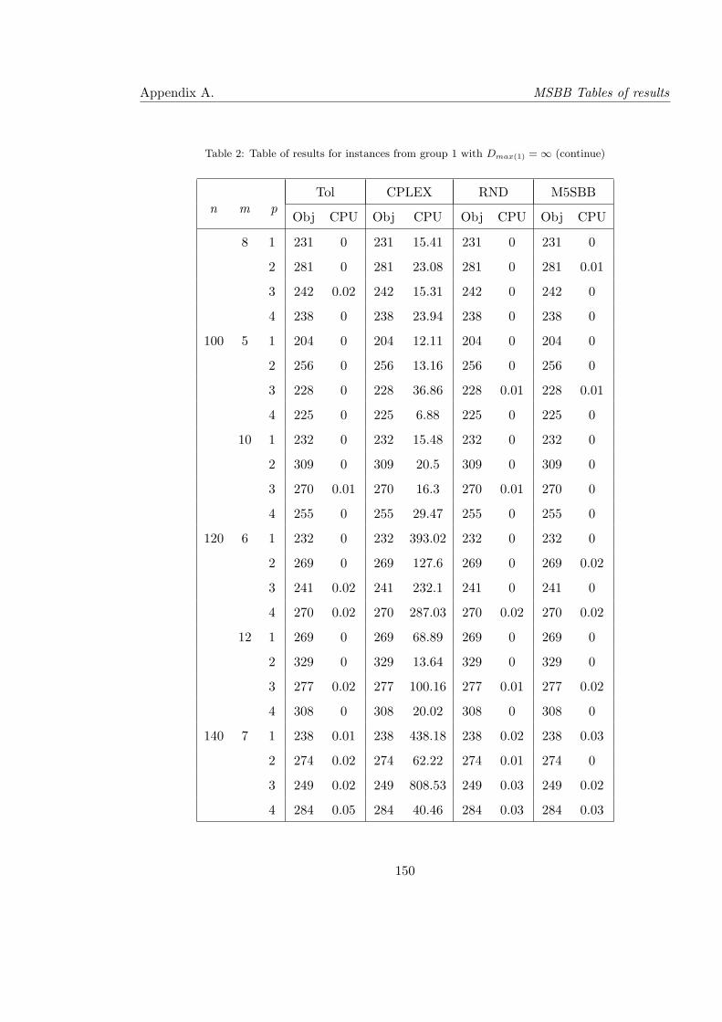
Appendix A. MSBB Tables of results
Table 2: Table of results for instances from group 1 with Dmax(1) = ∞ (continue)
Tol CPLEX RND M5SBBn m p
Obj CPU Obj CPU Obj CPU Obj CPU
8 1 231 0 231 15.41 231 0 231 0
2 281 0 281 23.08 281 0 281 0.01
3 242 0.02 242 15.31 242 0 242 0
4 238 0 238 23.94 238 0 238 0
100 5 1 204 0 204 12.11 204 0 204 0
2 256 0 256 13.16 256 0 256 0
3 228 0 228 36.86 228 0.01 228 0.01
4 225 0 225 6.88 225 0 225 0
10 1 232 0 232 15.48 232 0 232 0
2 309 0 309 20.5 309 0 309 0
3 270 0.01 270 16.3 270 0.01 270 0
4 255 0 255 29.47 255 0 255 0
120 6 1 232 0 232 393.02 232 0 232 0
2 269 0 269 127.6 269 0 269 0.02
3 241 0.02 241 232.1 241 0 241 0
4 270 0.02 270 287.03 270 0.02 270 0.02
12 1 269 0 269 68.89 269 0 269 0
2 329 0 329 13.64 329 0 329 0
3 277 0.02 277 100.16 277 0.01 277 0.02
4 308 0 308 20.02 308 0 308 0
140 7 1 238 0.01 238 438.18 238 0.02 238 0.03
2 274 0.02 274 62.22 274 0.01 274 0
3 249 0.02 249 808.53 249 0.03 249 0.02
4 284 0.05 284 40.46 284 0.03 284 0.03
150
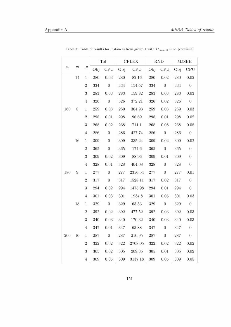
Appendix A. MSBB Tables of results
Table 3: Table of results for instances from group 1 with Dmax(1) = ∞ (continue)
Tol CPLEX RND M5SBBn m p
Obj CPU Obj CPU Obj CPU Obj CPU
14 1 280 0.03 280 82.16 280 0.02 280 0.02
2 334 0 334 154.57 334 0 334 0
3 283 0.03 283 159.82 283 0.03 283 0.03
4 326 0 326 372.21 326 0.02 326 0
160 8 1 259 0.03 259 364.93 259 0.03 259 0.03
2 298 0.01 298 96.69 298 0.01 298 0.02
3 268 0.02 268 711.1 268 0.08 268 0.08
4 286 0 286 427.74 286 0 286 0
16 1 309 0 309 335.24 309 0.02 309 0.02
2 365 0 365 174.6 365 0 365 0
3 309 0.02 309 88.96 309 0.01 309 0
4 328 0.01 328 404.08 328 0 328 0
180 9 1 277 0 277 2356.54 277 0 277 0.01
2 317 0 317 1528.11 317 0.02 317 0
3 294 0.02 294 1475.98 294 0.01 294 0
4 301 0.03 301 1934.8 301 0.05 301 0.03
18 1 329 0 329 65.53 329 0 329 0
2 392 0.02 392 477.52 392 0.03 392 0.03
3 340 0.03 340 170.32 340 0.03 340 0.03
4 347 0.01 347 63.88 347 0 347 0
200 10 1 287 0 287 210.95 287 0 287 0
2 322 0.02 322 2708.05 322 0.02 322 0.02
3 305 0.02 305 209.35 305 0.01 305 0.02
4 309 0.05 309 3137.18 309 0.05 309 0.05
151
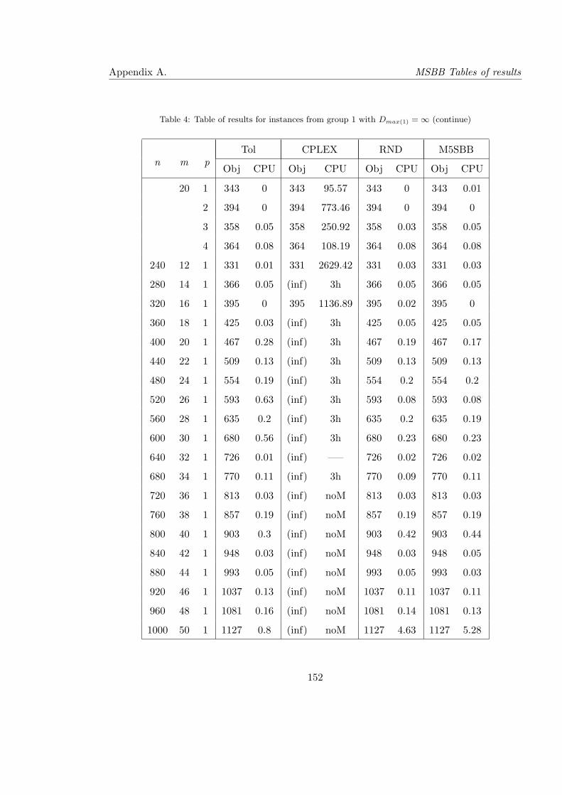
Appendix A. MSBB Tables of results
Table 4: Table of results for instances from group 1 with Dmax(1) = ∞ (continue)
Tol CPLEX RND M5SBBn m p
Obj CPU Obj CPU Obj CPU Obj CPU
20 1 343 0 343 95.57 343 0 343 0.01
2 394 0 394 773.46 394 0 394 0
3 358 0.05 358 250.92 358 0.03 358 0.05
4 364 0.08 364 108.19 364 0.08 364 0.08
240 12 1 331 0.01 331 2629.42 331 0.03 331 0.03
280 14 1 366 0.05 (inf) 3h 366 0.05 366 0.05
320 16 1 395 0 395 1136.89 395 0.02 395 0
360 18 1 425 0.03 (inf) 3h 425 0.05 425 0.05
400 20 1 467 0.28 (inf) 3h 467 0.19 467 0.17
440 22 1 509 0.13 (inf) 3h 509 0.13 509 0.13
480 24 1 554 0.19 (inf) 3h 554 0.2 554 0.2
520 26 1 593 0.63 (inf) 3h 593 0.08 593 0.08
560 28 1 635 0.2 (inf) 3h 635 0.2 635 0.19
600 30 1 680 0.56 (inf) 3h 680 0.23 680 0.23
640 32 1 726 0.01 (inf) —– 726 0.02 726 0.02
680 34 1 770 0.11 (inf) 3h 770 0.09 770 0.11
720 36 1 813 0.03 (inf) noM 813 0.03 813 0.03
760 38 1 857 0.19 (inf) noM 857 0.19 857 0.19
800 40 1 903 0.3 (inf) noM 903 0.42 903 0.44
840 42 1 948 0.03 (inf) noM 948 0.03 948 0.05
880 44 1 993 0.05 (inf) noM 993 0.05 993 0.03
920 46 1 1037 0.13 (inf) noM 1037 0.11 1037 0.11
960 48 1 1081 0.16 (inf) noM 1081 0.14 1081 0.13
1000 50 1 1127 0.8 (inf) noM 1127 4.63 1127 5.28
152
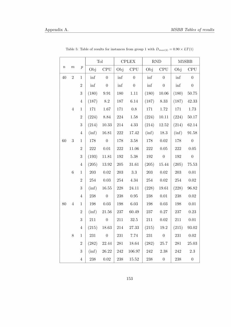
Appendix A. MSBB Tables of results
Table 5: Table of results for instances from group 1 with Dmax(2) = 0.90× LT (1)
Tol CPLEX RND M5SBBn m p
Obj CPU Obj CPU Obj CPU Obj CPU
40 2 1 inf 0 inf 0 inf 0 inf 0
2 inf 0 inf 0 inf 0 inf 0
3 (180) 9.91 180 1.11 (180) 10.06 (180) 50.75
4 (187) 8.2 187 6.14 (187) 8.33 (187) 42.33
4 1 171 1.67 171 0.8 171 1.72 171 1.73
2 (224) 8.84 224 1.58 (224) 10.11 (224) 50.17
3 (214) 10.33 214 4.33 (214) 12.52 (214) 62.14
4 (inf) 16.81 222 17.42 (inf) 18.3 (inf) 91.58
60 3 1 178 0 178 3.58 178 0.02 178 0
2 222 0.01 222 11.06 222 0.05 222 0.05
3 (193) 11.81 192 5.38 192 0 192 0
4 (205) 13.92 205 31.61 (205) 15.44 (205) 75.53
6 1 203 0.02 203 3.3 203 0.02 203 0.01
2 254 0.03 254 4.34 254 0.02 254 0.02
3 (inf) 16.55 228 24.11 (228) 19.61 (228) 96.82
4 238 0 238 0.95 238 0.01 238 0.02
80 4 1 198 0.03 198 6.03 198 0.03 198 0.01
2 (inf) 21.56 237 60.49 237 0.27 237 0.23
3 211 0 211 32.5 211 0.02 211 0.01
4 (215) 18.63 214 27.33 (215) 19.2 (215) 93.02
8 1 231 0 231 7.74 231 0 231 0.02
2 (282) 22.44 281 18.64 (282) 25.7 281 25.03
3 (inf) 26.22 242 106.97 242 2.38 242 2.3
4 238 0.02 238 15.52 238 0 238 0
153
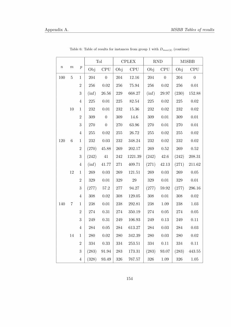
Appendix A. MSBB Tables of results
Table 6: Table of results for instances from group 1 with Dmax(2) (continue)
Tol CPLEX RND M5SBBn m p
Obj CPU Obj CPU Obj CPU Obj CPU
100 5 1 204 0 204 12.16 204 0 204 0
2 256 0.02 256 75.94 256 0.02 256 0.01
3 (inf) 26.56 229 668.27 (inf) 29.97 (230) 152.88
4 225 0.01 225 82.54 225 0.02 225 0.02
10 1 232 0.01 232 15.36 232 0.02 232 0.02
2 309 0 309 14.6 309 0.01 309 0.01
3 270 0 270 63.96 270 0.01 270 0.01
4 255 0.02 255 26.72 255 0.02 255 0.02
120 6 1 232 0.03 232 348.24 232 0.02 232 0.02
2 (270) 45.88 269 202.17 269 0.52 269 0.52
3 (242) 41 242 1221.39 (242) 42.6 (242) 208.31
4 (inf) 41.77 271 409.71 (271) 42.13 (271) 211.62
12 1 269 0.03 269 121.51 269 0.03 269 0.05
2 329 0.01 329 29 329 0.01 329 0.01
3 (277) 57.2 277 94.27 (277) 59.92 (277) 296.16
4 308 0.02 308 129.05 308 0.01 308 0.02
140 7 1 238 0.01 238 292.81 238 1.09 238 1.03
2 274 0.31 274 350.19 274 0.05 274 0.05
3 249 0.31 249 106.93 249 0.13 249 0.11
4 284 0.05 284 613.27 284 0.03 284 0.03
14 1 280 0.02 280 342.39 280 0.03 280 0.02
2 334 0.33 334 253.51 334 0.11 334 0.11
3 (283) 91.94 283 173.31 (283) 93.07 (283) 443.55
4 (328) 93.49 326 767.57 326 1.09 326 1.05
154
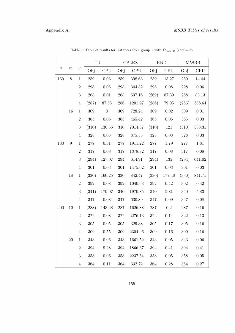
Appendix A. MSBB Tables of results
Table 7: Table of results for instances from group 1 with Dmax(2) (continue)
Tol CPLEX RND M5SBBn m p
Obj CPU Obj CPU Obj CPU Obj CPU
160 8 1 259 0.03 259 398.63 259 15.27 259 14.44
2 298 0.05 298 344.32 298 0.08 298 0.06
3 268 0.01 268 637.16 (269) 87.39 268 83.13
4 (287) 87.55 286 1201.97 (286) 79.05 (286) 386.64
16 1 309 0 309 728.24 309 0.02 309 0.01
2 365 0.05 365 465.42 365 0.05 365 0.03
3 (310) 130.55 310 7014.37 (310) 121 (310) 588.31
4 328 0.03 328 875.53 328 0.03 328 0.03
180 9 1 277 0.31 277 1911.22 277 1.79 277 1.81
2 317 0.08 317 1378.82 317 0.08 317 0.08
3 (294) 127.07 294 614.91 (294) 135 (294) 641.02
4 301 0.03 301 1475.62 301 0.03 301 0.03
18 1 (330) 160.25 330 842.47 (330) 177.48 (330) 841.71
2 392 0.08 392 1040.63 392 0.42 392 0.42
3 (341) 179.07 340 1970.85 340 5.81 340 5.83
4 347 0.08 347 630.89 347 0.09 347 0.08
200 10 1 (288) 143.28 287 1626.88 287 0.2 287 0.16
2 322 0.08 322 2276.13 322 0.14 322 0.13
3 305 0.05 305 329.38 305 0.17 305 0.16
4 309 0.55 309 2304.96 309 0.16 309 0.16
20 1 343 0.06 343 1661.52 343 0.05 343 0.06
2 394 9.28 394 1866.67 394 0.41 394 0.41
3 358 0.06 358 2237.54 358 0.05 358 0.05
4 364 0.11 364 332.72 364 0.28 364 0.27
155
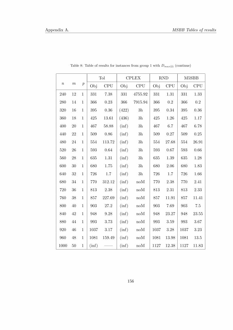
Appendix A. MSBB Tables of results
Table 8: Table of results for instances from group 1 with Dmax(2) (continue)
Tol CPLEX RND M5SBBn m p
Obj CPU Obj CPU Obj CPU Obj CPU
240 12 1 331 7.38 331 4755.92 331 1.31 331 1.33
280 14 1 366 0.23 366 7915.94 366 0.2 366 0.2
320 16 1 395 0.36 (422) 3h 395 0.34 395 0.36
360 18 1 425 13.61 (436) 3h 425 1.26 425 1.17
400 20 1 467 58.88 (inf) 3h 467 6.7 467 6.78
440 22 1 509 0.86 (inf) 3h 509 0.27 509 0.25
480 24 1 554 113.72 (inf) 3h 554 27.68 554 26.91
520 26 1 593 0.64 (inf) 3h 593 0.67 593 0.66
560 28 1 635 1.31 (inf) 3h 635 1.39 635 1.28
600 30 1 680 1.75 (inf) 3h 680 2.06 680 1.83
640 32 1 726 1.7 (inf) 3h 726 1.7 726 1.66
680 34 1 770 312.12 (inf) noM 770 2.38 770 2.41
720 36 1 813 2.38 (inf) noM 813 2.31 813 2.33
760 38 1 857 227.69 (inf) noM 857 11.91 857 11.41
800 40 1 903 27.2 (inf) noM 903 7.69 903 7.5
840 42 1 948 9.28 (inf) noM 948 23.27 948 23.55
880 44 1 993 3.73 (inf) noM 993 3.59 993 3.67
920 46 1 1037 3.17 (inf) noM 1037 3.28 1037 3.23
960 48 1 1081 159.49 (inf) noM 1081 13.98 1081 13.5
1000 50 1 (inf) —— (inf) noM 1127 12.38 1127 11.83
156
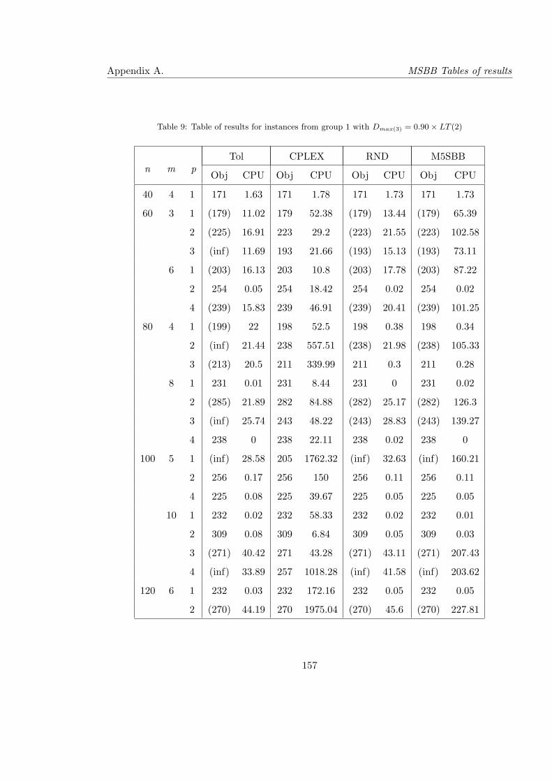
Appendix A. MSBB Tables of results
Table 9: Table of results for instances from group 1 with Dmax(3) = 0.90× LT (2)
Tol CPLEX RND M5SBBn m p
Obj CPU Obj CPU Obj CPU Obj CPU
40 4 1 171 1.63 171 1.78 171 1.73 171 1.73
60 3 1 (179) 11.02 179 52.38 (179) 13.44 (179) 65.39
2 (225) 16.91 223 29.2 (223) 21.55 (223) 102.58
3 (inf) 11.69 193 21.66 (193) 15.13 (193) 73.11
6 1 (203) 16.13 203 10.8 (203) 17.78 (203) 87.22
2 254 0.05 254 18.42 254 0.02 254 0.02
4 (239) 15.83 239 46.91 (239) 20.41 (239) 101.25
80 4 1 (199) 22 198 52.5 198 0.38 198 0.34
2 (inf) 21.44 238 557.51 (238) 21.98 (238) 105.33
3 (213) 20.5 211 339.99 211 0.3 211 0.28
8 1 231 0.01 231 8.44 231 0 231 0.02
2 (285) 21.89 282 84.88 (282) 25.17 (282) 126.3
3 (inf) 25.74 243 48.22 (243) 28.83 (243) 139.27
4 238 0 238 22.11 238 0.02 238 0
100 5 1 (inf) 28.58 205 1762.32 (inf) 32.63 (inf) 160.21
2 256 0.17 256 150 256 0.11 256 0.11
4 225 0.08 225 39.67 225 0.05 225 0.05
10 1 232 0.02 232 58.33 232 0.02 232 0.01
2 309 0.08 309 6.84 309 0.05 309 0.03
3 (271) 40.42 271 43.28 (271) 43.11 (271) 207.43
4 (inf) 33.89 257 1018.28 (inf) 41.58 (inf) 203.62
120 6 1 232 0.03 232 172.16 232 0.05 232 0.05
2 (270) 44.19 270 1975.04 (270) 45.6 (270) 227.81
157
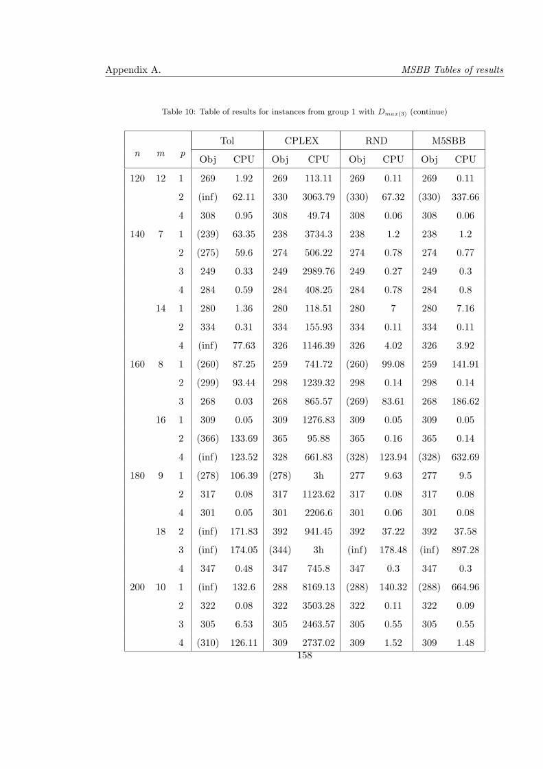
Appendix A. MSBB Tables of results
Table 10: Table of results for instances from group 1 with Dmax(3) (continue)
Tol CPLEX RND M5SBBn m p
Obj CPU Obj CPU Obj CPU Obj CPU
120 12 1 269 1.92 269 113.11 269 0.11 269 0.11
2 (inf) 62.11 330 3063.79 (330) 67.32 (330) 337.66
4 308 0.95 308 49.74 308 0.06 308 0.06
140 7 1 (239) 63.35 238 3734.3 238 1.2 238 1.2
2 (275) 59.6 274 506.22 274 0.78 274 0.77
3 249 0.33 249 2989.76 249 0.27 249 0.3
4 284 0.59 284 408.25 284 0.78 284 0.8
14 1 280 1.36 280 118.51 280 7 280 7.16
2 334 0.31 334 155.93 334 0.11 334 0.11
4 (inf) 77.63 326 1146.39 326 4.02 326 3.92
160 8 1 (260) 87.25 259 741.72 (260) 99.08 259 141.91
2 (299) 93.44 298 1239.32 298 0.14 298 0.14
3 268 0.03 268 865.57 (269) 83.61 268 186.62
16 1 309 0.05 309 1276.83 309 0.05 309 0.05
2 (366) 133.69 365 95.88 365 0.16 365 0.14
4 (inf) 123.52 328 661.83 (328) 123.94 (328) 632.69
180 9 1 (278) 106.39 (278) 3h 277 9.63 277 9.5
2 317 0.08 317 1123.62 317 0.08 317 0.08
4 301 0.05 301 2206.6 301 0.06 301 0.08
18 2 (inf) 171.83 392 941.45 392 37.22 392 37.58
3 (inf) 174.05 (344) 3h (inf) 178.48 (inf) 897.28
4 347 0.48 347 745.8 347 0.3 347 0.3
200 10 1 (inf) 132.6 288 8169.13 (288) 140.32 (288) 664.96
2 322 0.08 322 3503.28 322 0.11 322 0.09
3 305 6.53 305 2463.57 305 0.55 305 0.55
4 (310) 126.11 309 2737.02 309 1.52 309 1.48158
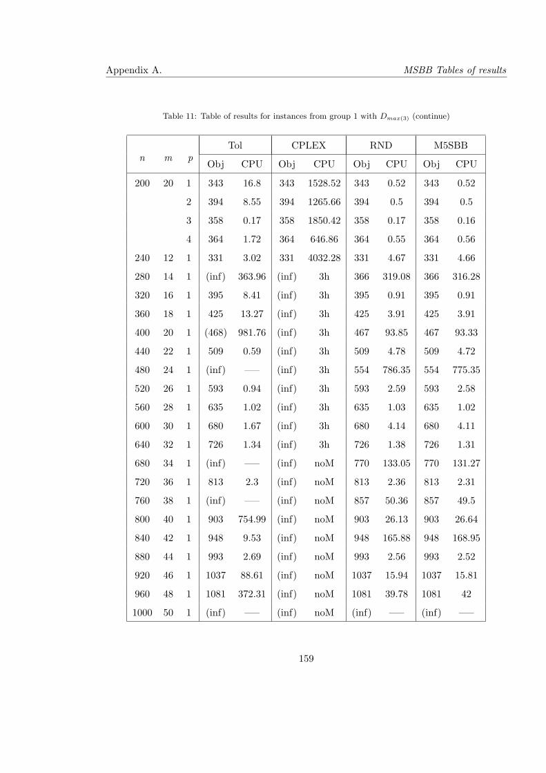
Appendix A. MSBB Tables of results
Table 11: Table of results for instances from group 1 with Dmax(3) (continue)
Tol CPLEX RND M5SBBn m p
Obj CPU Obj CPU Obj CPU Obj CPU
200 20 1 343 16.8 343 1528.52 343 0.52 343 0.52
2 394 8.55 394 1265.66 394 0.5 394 0.5
3 358 0.17 358 1850.42 358 0.17 358 0.16
4 364 1.72 364 646.86 364 0.55 364 0.56
240 12 1 331 3.02 331 4032.28 331 4.67 331 4.66
280 14 1 (inf) 363.96 (inf) 3h 366 319.08 366 316.28
320 16 1 395 8.41 (inf) 3h 395 0.91 395 0.91
360 18 1 425 13.27 (inf) 3h 425 3.91 425 3.91
400 20 1 (468) 981.76 (inf) 3h 467 93.85 467 93.33
440 22 1 509 0.59 (inf) 3h 509 4.78 509 4.72
480 24 1 (inf) —– (inf) 3h 554 786.35 554 775.35
520 26 1 593 0.94 (inf) 3h 593 2.59 593 2.58
560 28 1 635 1.02 (inf) 3h 635 1.03 635 1.02
600 30 1 680 1.67 (inf) 3h 680 4.14 680 4.11
640 32 1 726 1.34 (inf) 3h 726 1.38 726 1.31
680 34 1 (inf) —– (inf) noM 770 133.05 770 131.27
720 36 1 813 2.3 (inf) noM 813 2.36 813 2.31
760 38 1 (inf) —– (inf) noM 857 50.36 857 49.5
800 40 1 903 754.99 (inf) noM 903 26.13 903 26.64
840 42 1 948 9.53 (inf) noM 948 165.88 948 168.95
880 44 1 993 2.69 (inf) noM 993 2.56 993 2.52
920 46 1 1037 88.61 (inf) noM 1037 15.94 1037 15.81
960 48 1 1081 372.31 (inf) noM 1081 39.78 1081 42
1000 50 1 (inf) —– (inf) noM (inf) —– (inf) —–
159

Appendix A. MSBB Tables of results
.2 Tables of Results for Group 2
Table 12: Table of results for instances from group 2 with Dmax(1) = ∞Tol CPLEX RND M5SBB
n m pObj CPU Obj CPU Obj CPU Obj CPU
40 2 1 1323 0.03 1323 0.59 1323 0.02 1323 0.03
2 1898 0 1898 0.5 1898 0 1898 0
3 1586 0 1586 0.5 1586 0 1586 0
4 1690 0 1690 0.7 1690 0 1690 0
4 1 1483 0 1483 0.5 1483 0 1483 0
2 2034 0 2034 0.42 2034 0 2034 0.01
3 1930 0 1930 0.28 1930 0 1930 0
4 1999 0 1999 0.81 1999 0 1999 0
60 3 1 1478 13.09 1478 3.09 1478 14.81 1478 15.7
2 1895 0 1895 5.2 1895 0 1895 0
3 1660 11.14 1660 1.08 1660 0.58 1660 0.58
4 1739 0 1739 2.11 1739 0 1739 0
6 1 1686 0.01 1686 1.48 1686 0.02 1686 0.02
2 2153 0 2153 3.53 2153 0 2153 0
3 1993 0.01 1993 4.16 1993 0 1993 0.02
4 2041 0 2041 0.77 2041 0 2041 0
80 4 1 1529 0 1529 5.66 1529 0 1529 0
2 (1930) 26.8 1907 11.69 (1930) 29.27 (1930) 150.65
3 1712 0.02 1712 45.3 1712 0 1712 0
4 1720 0 1720 1.83 1720 0 1720 0
8 1 1837 0 1837 4.81 1837 0 1837 0
2 (2235) 30.81 2235 9.75 (2235) 33.28 (2235) 170.07
3 1995 0 1995 7.59 1995 0 1995 0
4 1917 0 1917 6.61 1917 0 1917 0
160
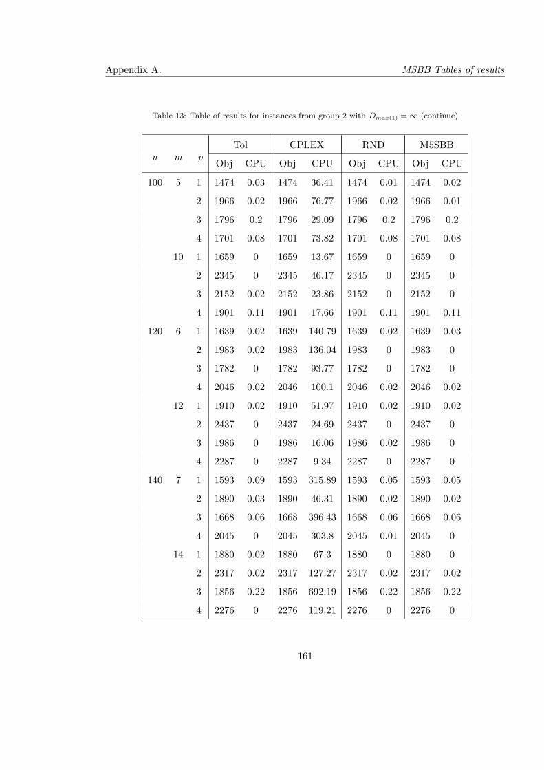
Appendix A. MSBB Tables of results
Table 13: Table of results for instances from group 2 with Dmax(1) = ∞ (continue)
Tol CPLEX RND M5SBBn m p
Obj CPU Obj CPU Obj CPU Obj CPU
100 5 1 1474 0.03 1474 36.41 1474 0.01 1474 0.02
2 1966 0.02 1966 76.77 1966 0.02 1966 0.01
3 1796 0.2 1796 29.09 1796 0.2 1796 0.2
4 1701 0.08 1701 73.82 1701 0.08 1701 0.08
10 1 1659 0 1659 13.67 1659 0 1659 0
2 2345 0 2345 46.17 2345 0 2345 0
3 2152 0.02 2152 23.86 2152 0 2152 0
4 1901 0.11 1901 17.66 1901 0.11 1901 0.11
120 6 1 1639 0.02 1639 140.79 1639 0.02 1639 0.03
2 1983 0.02 1983 136.04 1983 0 1983 0
3 1782 0 1782 93.77 1782 0 1782 0
4 2046 0.02 2046 100.1 2046 0.02 2046 0.02
12 1 1910 0.02 1910 51.97 1910 0.02 1910 0.02
2 2437 0 2437 24.69 2437 0 2437 0
3 1986 0 1986 16.06 1986 0.02 1986 0
4 2287 0 2287 9.34 2287 0 2287 0
140 7 1 1593 0.09 1593 315.89 1593 0.05 1593 0.05
2 1890 0.03 1890 46.31 1890 0.02 1890 0.02
3 1668 0.06 1668 396.43 1668 0.06 1668 0.06
4 2045 0 2045 303.8 2045 0.01 2045 0
14 1 1880 0.02 1880 67.3 1880 0 1880 0
2 2317 0.02 2317 127.27 2317 0.02 2317 0.02
3 1856 0.22 1856 692.19 1856 0.22 1856 0.22
4 2276 0 2276 119.21 2276 0 2276 0
161
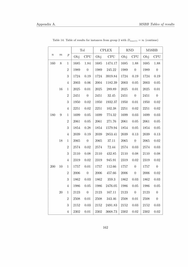
Appendix A. MSBB Tables of results
Table 14: Table of results for instances from group 2 with Dmax(1) = ∞ (continue)
Tol CPLEX RND M5SBBn m p
Obj CPU Obj CPU Obj CPU Obj CPU
160 8 1 1685 1.84 1685 1474.17 1685 1.88 1685 1.88
2 1989 0 1989 245.22 1989 0 1989 0
3 1724 0.19 1724 3919.84 1724 0.19 1724 0.19
4 2003 0.06 2004 1182.39 2003 0.05 2003 0.05
16 1 2025 0.01 2025 289.89 2025 0.01 2025 0.01
2 2451 0 2451 32.45 2451 0 2451 0
3 1950 0.02 1950 1932.37 1950 0.01 1950 0.02
4 2251 0.02 2251 102.38 2251 0.02 2251 0.02
180 9 1 1699 0.05 1699 774.32 1699 0.03 1699 0.03
2 2061 0.05 2061 271.76 2061 0.05 2061 0.05
3 1854 0.28 1854 1579.94 1854 0.05 1854 0.05
4 2039 0.19 2039 2853.41 2039 0.13 2039 0.13
18 1 2065 0 2065 37.11 2065 0 2065 0.02
2 2574 0.02 2574 72.44 2574 0.03 2574 0.03
3 2110 0.08 2110 432.85 2110 0.08 2110 0.08
4 2319 0.02 2319 945.91 2319 0.02 2319 0.02
200 10 1 1757 0.01 1757 112.66 1757 0 1757 0
2 2006 0 2006 457.66 2006 0 2006 0.02
3 1862 0.03 1862 359.3 1862 0.03 1862 0.03
4 1986 0.05 1986 2476.05 1986 0.05 1986 0.05
20 1 2123 0 2123 167.11 2123 0 2123 0
2 2508 0.01 2508 343.46 2508 0.01 2508 0
3 2152 0.03 2152 2491.83 2152 0.03 2152 0.03
4 2302 0.01 2302 3668.73 2302 0.02 2302 0.02
162
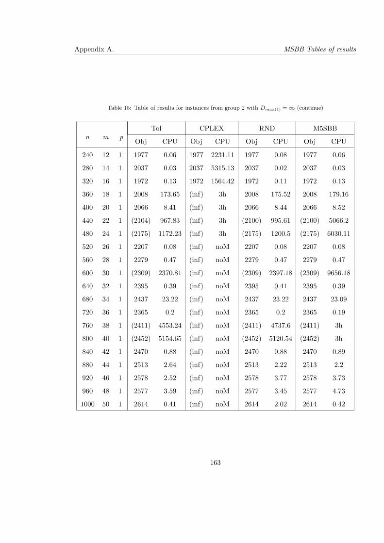
Appendix A. MSBB Tables of results
Table 15: Table of results for instances from group 2 with Dmax(1) = ∞ (continue)
Tol CPLEX RND M5SBBn m p
Obj CPU Obj CPU Obj CPU Obj CPU
240 12 1 1977 0.06 1977 2231.11 1977 0.08 1977 0.06
280 14 1 2037 0.03 2037 5315.13 2037 0.02 2037 0.03
320 16 1 1972 0.13 1972 1564.42 1972 0.11 1972 0.13
360 18 1 2008 173.65 (inf) 3h 2008 175.52 2008 179.16
400 20 1 2066 8.41 (inf) 3h 2066 8.44 2066 8.52
440 22 1 (2104) 967.83 (inf) 3h (2100) 995.61 (2100) 5066.2
480 24 1 (2175) 1172.23 (inf) 3h (2175) 1200.5 (2175) 6030.11
520 26 1 2207 0.08 (inf) noM 2207 0.08 2207 0.08
560 28 1 2279 0.47 (inf) noM 2279 0.47 2279 0.47
600 30 1 (2309) 2370.81 (inf) noM (2309) 2397.18 (2309) 9656.18
640 32 1 2395 0.39 (inf) noM 2395 0.41 2395 0.39
680 34 1 2437 23.22 (inf) noM 2437 23.22 2437 23.09
720 36 1 2365 0.2 (inf) noM 2365 0.2 2365 0.19
760 38 1 (2411) 4553.24 (inf) noM (2411) 4737.6 (2411) 3h
800 40 1 (2452) 5154.65 (inf) noM (2452) 5120.54 (2452) 3h
840 42 1 2470 0.88 (inf) noM 2470 0.88 2470 0.89
880 44 1 2513 2.64 (inf) noM 2513 2.22 2513 2.2
920 46 1 2578 2.52 (inf) noM 2578 3.77 2578 3.73
960 48 1 2577 3.59 (inf) noM 2577 3.45 2577 4.73
1000 50 1 2614 0.41 (inf) noM 2614 2.02 2614 0.42
163
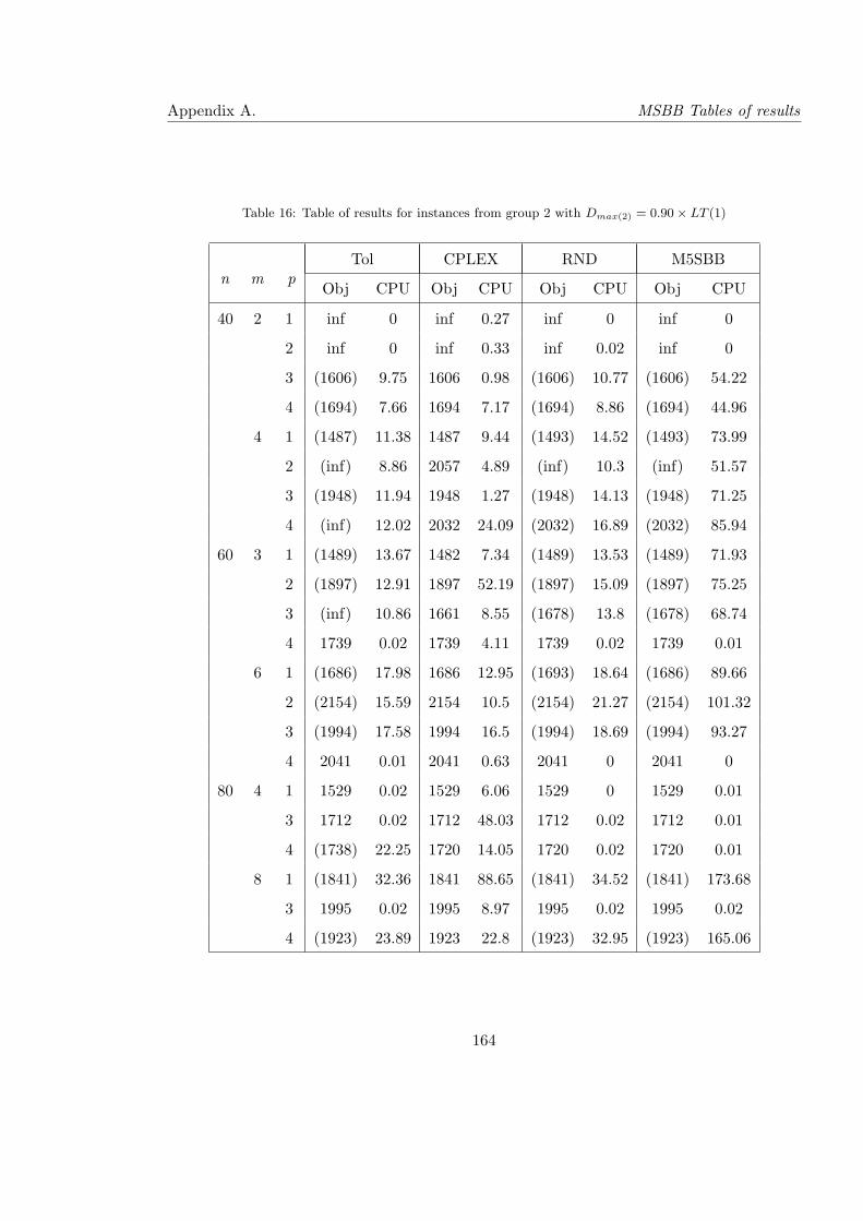
Appendix A. MSBB Tables of results
Table 16: Table of results for instances from group 2 with Dmax(2) = 0.90× LT (1)
Tol CPLEX RND M5SBBn m p
Obj CPU Obj CPU Obj CPU Obj CPU
40 2 1 inf 0 inf 0.27 inf 0 inf 0
2 inf 0 inf 0.33 inf 0.02 inf 0
3 (1606) 9.75 1606 0.98 (1606) 10.77 (1606) 54.22
4 (1694) 7.66 1694 7.17 (1694) 8.86 (1694) 44.96
4 1 (1487) 11.38 1487 9.44 (1493) 14.52 (1493) 73.99
2 (inf) 8.86 2057 4.89 (inf) 10.3 (inf) 51.57
3 (1948) 11.94 1948 1.27 (1948) 14.13 (1948) 71.25
4 (inf) 12.02 2032 24.09 (2032) 16.89 (2032) 85.94
60 3 1 (1489) 13.67 1482 7.34 (1489) 13.53 (1489) 71.93
2 (1897) 12.91 1897 52.19 (1897) 15.09 (1897) 75.25
3 (inf) 10.86 1661 8.55 (1678) 13.8 (1678) 68.74
4 1739 0.02 1739 4.11 1739 0.02 1739 0.01
6 1 (1686) 17.98 1686 12.95 (1693) 18.64 (1686) 89.66
2 (2154) 15.59 2154 10.5 (2154) 21.27 (2154) 101.32
3 (1994) 17.58 1994 16.5 (1994) 18.69 (1994) 93.27
4 2041 0.01 2041 0.63 2041 0 2041 0
80 4 1 1529 0.02 1529 6.06 1529 0 1529 0.01
3 1712 0.02 1712 48.03 1712 0.02 1712 0.01
4 (1738) 22.25 1720 14.05 1720 0.02 1720 0.01
8 1 (1841) 32.36 1841 88.65 (1841) 34.52 (1841) 173.68
3 1995 0.02 1995 8.97 1995 0.02 1995 0.02
4 (1923) 23.89 1923 22.8 (1923) 32.95 (1923) 165.06
164
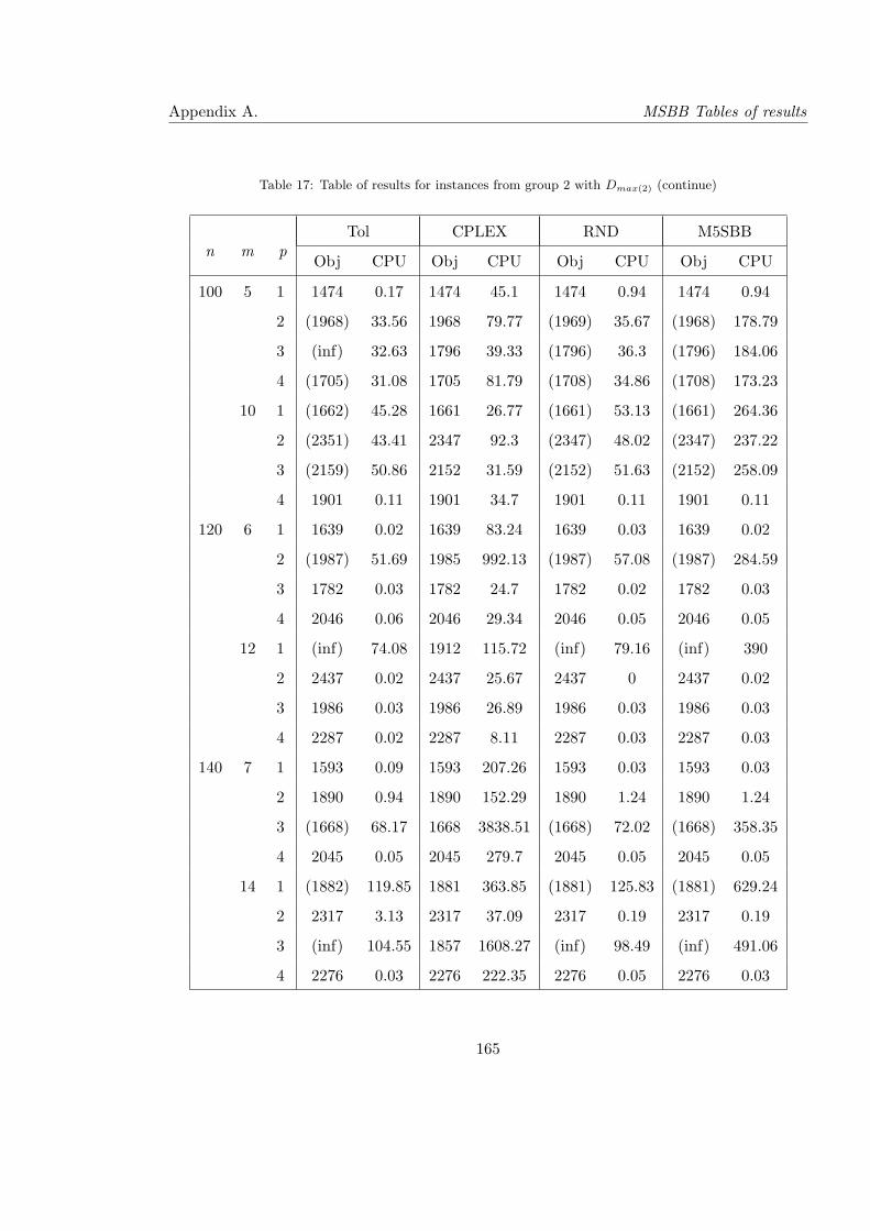
Appendix A. MSBB Tables of results
Table 17: Table of results for instances from group 2 with Dmax(2) (continue)
Tol CPLEX RND M5SBBn m p
Obj CPU Obj CPU Obj CPU Obj CPU
100 5 1 1474 0.17 1474 45.1 1474 0.94 1474 0.94
2 (1968) 33.56 1968 79.77 (1969) 35.67 (1968) 178.79
3 (inf) 32.63 1796 39.33 (1796) 36.3 (1796) 184.06
4 (1705) 31.08 1705 81.79 (1708) 34.86 (1708) 173.23
10 1 (1662) 45.28 1661 26.77 (1661) 53.13 (1661) 264.36
2 (2351) 43.41 2347 92.3 (2347) 48.02 (2347) 237.22
3 (2159) 50.86 2152 31.59 (2152) 51.63 (2152) 258.09
4 1901 0.11 1901 34.7 1901 0.11 1901 0.11
120 6 1 1639 0.02 1639 83.24 1639 0.03 1639 0.02
2 (1987) 51.69 1985 992.13 (1987) 57.08 (1987) 284.59
3 1782 0.03 1782 24.7 1782 0.02 1782 0.03
4 2046 0.06 2046 29.34 2046 0.05 2046 0.05
12 1 (inf) 74.08 1912 115.72 (inf) 79.16 (inf) 390
2 2437 0.02 2437 25.67 2437 0 2437 0.02
3 1986 0.03 1986 26.89 1986 0.03 1986 0.03
4 2287 0.02 2287 8.11 2287 0.03 2287 0.03
140 7 1 1593 0.09 1593 207.26 1593 0.03 1593 0.03
2 1890 0.94 1890 152.29 1890 1.24 1890 1.24
3 (1668) 68.17 1668 3838.51 (1668) 72.02 (1668) 358.35
4 2045 0.05 2045 279.7 2045 0.05 2045 0.05
14 1 (1882) 119.85 1881 363.85 (1881) 125.83 (1881) 629.24
2 2317 3.13 2317 37.09 2317 0.19 2317 0.19
3 (inf) 104.55 1857 1608.27 (inf) 98.49 (inf) 491.06
4 2276 0.03 2276 222.35 2276 0.05 2276 0.03
165
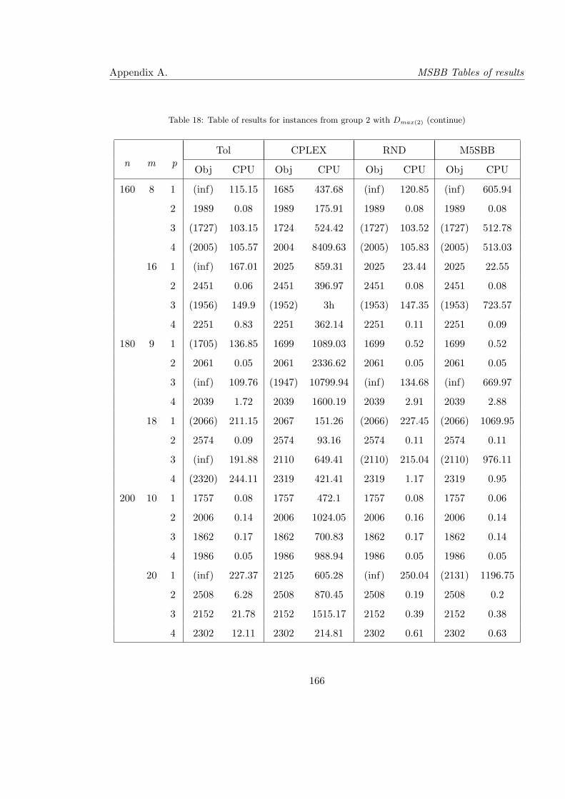
Appendix A. MSBB Tables of results
Table 18: Table of results for instances from group 2 with Dmax(2) (continue)
Tol CPLEX RND M5SBBn m p
Obj CPU Obj CPU Obj CPU Obj CPU
160 8 1 (inf) 115.15 1685 437.68 (inf) 120.85 (inf) 605.94
2 1989 0.08 1989 175.91 1989 0.08 1989 0.08
3 (1727) 103.15 1724 524.42 (1727) 103.52 (1727) 512.78
4 (2005) 105.57 2004 8409.63 (2005) 105.83 (2005) 513.03
16 1 (inf) 167.01 2025 859.31 2025 23.44 2025 22.55
2 2451 0.06 2451 396.97 2451 0.08 2451 0.08
3 (1956) 149.9 (1952) 3h (1953) 147.35 (1953) 723.57
4 2251 0.83 2251 362.14 2251 0.11 2251 0.09
180 9 1 (1705) 136.85 1699 1089.03 1699 0.52 1699 0.52
2 2061 0.05 2061 2336.62 2061 0.05 2061 0.05
3 (inf) 109.76 (1947) 10799.94 (inf) 134.68 (inf) 669.97
4 2039 1.72 2039 1600.19 2039 2.91 2039 2.88
18 1 (2066) 211.15 2067 151.26 (2066) 227.45 (2066) 1069.95
2 2574 0.09 2574 93.16 2574 0.11 2574 0.11
3 (inf) 191.88 2110 649.41 (2110) 215.04 (2110) 976.11
4 (2320) 244.11 2319 421.41 2319 1.17 2319 0.95
200 10 1 1757 0.08 1757 472.1 1757 0.08 1757 0.06
2 2006 0.14 2006 1024.05 2006 0.16 2006 0.14
3 1862 0.17 1862 700.83 1862 0.17 1862 0.14
4 1986 0.05 1986 988.94 1986 0.05 1986 0.05
20 1 (inf) 227.37 2125 605.28 (inf) 250.04 (2131) 1196.75
2 2508 6.28 2508 870.45 2508 0.19 2508 0.2
3 2152 21.78 2152 1515.17 2152 0.39 2152 0.38
4 2302 12.11 2302 214.81 2302 0.61 2302 0.63
166
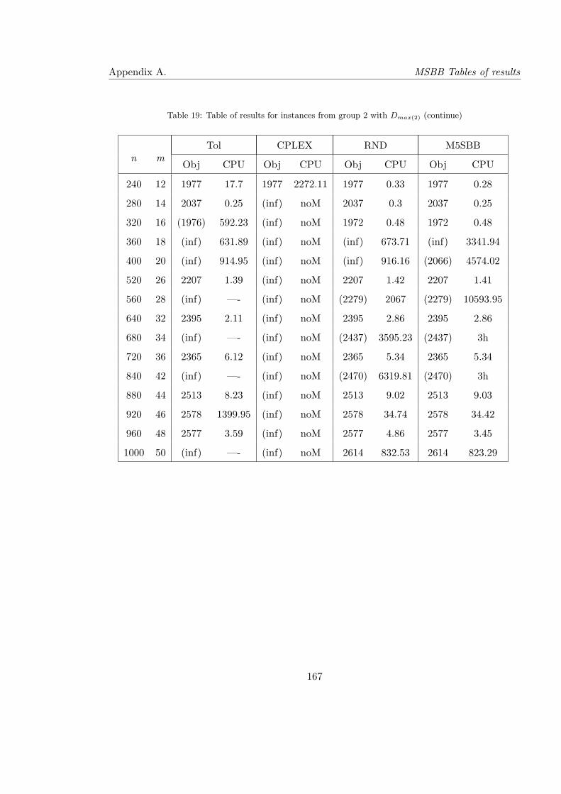
Appendix A. MSBB Tables of results
Table 19: Table of results for instances from group 2 with Dmax(2) (continue)
Tol CPLEX RND M5SBBn m
Obj CPU Obj CPU Obj CPU Obj CPU
240 12 1977 17.7 1977 2272.11 1977 0.33 1977 0.28
280 14 2037 0.25 (inf) noM 2037 0.3 2037 0.25
320 16 (1976) 592.23 (inf) noM 1972 0.48 1972 0.48
360 18 (inf) 631.89 (inf) noM (inf) 673.71 (inf) 3341.94
400 20 (inf) 914.95 (inf) noM (inf) 916.16 (2066) 4574.02
520 26 2207 1.39 (inf) noM 2207 1.42 2207 1.41
560 28 (inf) —- (inf) noM (2279) 2067 (2279) 10593.95
640 32 2395 2.11 (inf) noM 2395 2.86 2395 2.86
680 34 (inf) —- (inf) noM (2437) 3595.23 (2437) 3h
720 36 2365 6.12 (inf) noM 2365 5.34 2365 5.34
840 42 (inf) —- (inf) noM (2470) 6319.81 (2470) 3h
880 44 2513 8.23 (inf) noM 2513 9.02 2513 9.03
920 46 2578 1399.95 (inf) noM 2578 34.74 2578 34.42
960 48 2577 3.59 (inf) noM 2577 4.86 2577 3.45
1000 50 (inf) —- (inf) noM 2614 832.53 2614 823.29
167
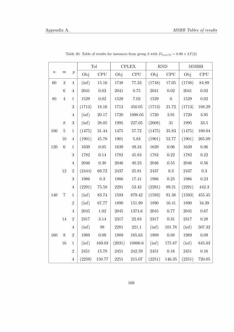
Appendix A. MSBB Tables of results
Table 20: Table of results for instances from group 2 with Dmax(3) = 0.90× LT (2)
Tol CPLEX RND M5SBBn m p
Obj CPU Obj CPU Obj CPU Obj CPU
60 3 4 (inf) 15.16 1748 77.33 (1748) 17.05 (1748) 84.89
6 4 2041 0.03 2041 0.75 2041 0.02 2041 0.02
80 4 1 1529 0.02 1529 7.02 1529 0 1529 0.02
3 (1713) 18.16 1713 450.05 (1713) 21.72 (1713) 108.29
4 (inf) 20.17 1720 1098.05 1720 3.91 1720 3.95
8 3 (inf) 28.05 1995 227.05 (2008) 31 1995 33.5
100 5 1 (1475) 31.44 1475 57.72 (1475) 35.83 (1475) 180.04
10 4 (1901) 45.78 1901 5.83 (1901) 52.77 (1901) 265.09
120 6 1 1639 0.05 1639 49.34 1639 0.06 1639 0.06
3 1782 0.14 1782 45.83 1782 0.22 1782 0.22
4 2046 0.38 2046 40.23 2046 0.55 2046 0.56
12 2 (2444) 69.72 2437 25.81 2437 0.3 2437 0.3
3 1986 0.3 1986 17.41 1986 0.25 1986 0.23
4 (2291) 75.58 2291 53.42 (2291) 89.21 (2291) 442.3
140 7 1 (inf) 83.74 1593 879.42 (1593) 91.38 (1593) 455.45
2 (inf) 67.77 1890 151.99 1890 16.41 1890 16.39
4 2045 1.02 2045 1374.6 2045 0.77 2045 0.67
14 2 2317 3.14 2317 22.83 2317 0.31 2317 0.28
4 (inf) 98 2281 221.1 (inf) 101.76 (inf) 507.32
160 8 2 1989 0.09 1989 105.63 1989 0.08 1989 0.09
16 1 (inf) 169.03 (2031) 10800.6 (inf) 175.87 (inf) 845.03
2 2451 15.78 2451 242.59 2451 0.16 2451 0.16
4 (2259) 150.77 2251 215.07 (2251) 146.35 (2251) 720.05
168
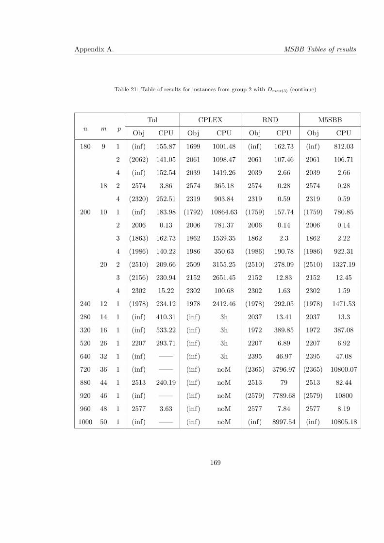
Appendix A. MSBB Tables of results
Table 21: Table of results for instances from group 2 with Dmax(3) (continue)
Tol CPLEX RND M5SBBn m p
Obj CPU Obj CPU Obj CPU Obj CPU
180 9 1 (inf) 155.87 1699 1001.48 (inf) 162.73 (inf) 812.03
2 (2062) 141.05 2061 1098.47 2061 107.46 2061 106.71
4 (inf) 152.54 2039 1419.26 2039 2.66 2039 2.66
18 2 2574 3.86 2574 365.18 2574 0.28 2574 0.28
4 (2320) 252.51 2319 903.84 2319 0.59 2319 0.59
200 10 1 (inf) 183.98 (1792) 10864.63 (1759) 157.74 (1759) 780.85
2 2006 0.13 2006 781.37 2006 0.14 2006 0.14
3 (1863) 162.73 1862 1539.35 1862 2.3 1862 2.22
4 (1986) 140.22 1986 350.63 (1986) 190.78 (1986) 922.31
20 2 (2510) 209.66 2509 3155.25 (2510) 278.09 (2510) 1327.19
3 (2156) 230.94 2152 2651.45 2152 12.83 2152 12.45
4 2302 15.22 2302 100.68 2302 1.63 2302 1.59
240 12 1 (1978) 234.12 1978 2412.46 (1978) 292.05 (1978) 1471.53
280 14 1 (inf) 410.31 (inf) 3h 2037 13.41 2037 13.3
320 16 1 (inf) 533.22 (inf) 3h 1972 389.85 1972 387.08
520 26 1 2207 293.71 (inf) 3h 2207 6.89 2207 6.92
640 32 1 (inf) —— (inf) 3h 2395 46.97 2395 47.08
720 36 1 (inf) —— (inf) noM (2365) 3796.97 (2365) 10800.07
880 44 1 2513 240.19 (inf) noM 2513 79 2513 82.44
920 46 1 (inf) —— (inf) noM (2579) 7789.68 (2579) 10800
960 48 1 2577 3.63 (inf) noM 2577 7.84 2577 8.19
1000 50 1 (inf) —— (inf) noM (inf) 8997.54 (inf) 10805.18
169
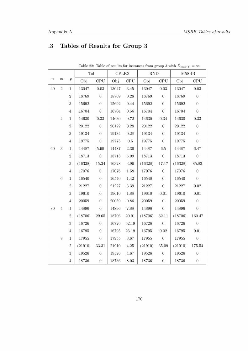
Appendix A. MSBB Tables of results
.3 Tables of Results for Group 3
Table 22: Table of results for instances from group 3 with Dmax(1) = ∞Tol CPLEX RND M5SBB
n m pObj CPU Obj CPU Obj CPU Obj CPU
40 2 1 13047 0.03 13047 3.45 13047 0.03 13047 0.03
2 18769 0 18769 0.28 18769 0 18769 0
3 15692 0 15692 0.44 15692 0 15692 0
4 16704 0 16704 0.56 16704 0 16704 0
4 1 14630 0.33 14630 0.72 14630 0.34 14630 0.33
2 20122 0 20122 0.28 20122 0 20122 0
3 19134 0 19134 0.28 19134 0 19134 0
4 19775 0 19775 0.5 19775 0 19775 0
60 3 1 14487 5.99 14487 2.36 14487 6.5 14487 6.47
2 18713 0 18713 5.99 18713 0 18713 0
3 (16328) 15.24 16328 3.96 (16328) 17.17 (16328) 85.83
4 17076 0 17076 1.58 17076 0 17076 0
6 1 16540 0 16540 1.42 16540 0 16540 0
2 21227 0 21227 3.39 21227 0 21227 0.02
3 19610 0 19610 1.88 19610 0.01 19610 0.01
4 20059 0 20059 0.86 20059 0 20059 0
80 4 1 14896 0 14896 7.88 14896 0 14896 0
2 (18706) 29.65 18706 20.91 (18706) 32.11 (18706) 160.47
3 16726 0 16726 62.19 16726 0 16726 0
4 16795 0 16795 23.19 16795 0.02 16795 0.01
8 1 17955 0 17955 3.67 17955 0 17955 0
2 (21910) 33.31 21910 4.25 (21910) 35.09 (21910) 175.54
3 19526 0 19526 4.67 19526 0 19526 0
4 18736 0 18736 8.03 18736 0 18736 0
170
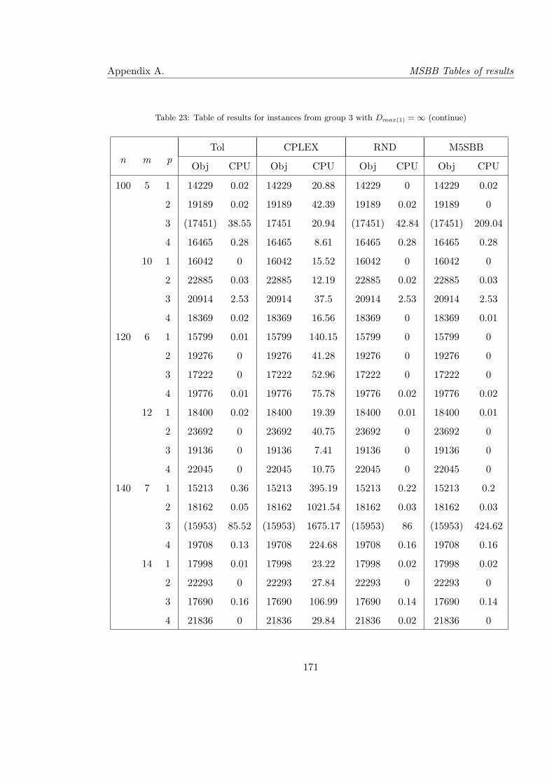
Appendix A. MSBB Tables of results
Table 23: Table of results for instances from group 3 with Dmax(1) = ∞ (continue)
Tol CPLEX RND M5SBBn m p
Obj CPU Obj CPU Obj CPU Obj CPU
100 5 1 14229 0.02 14229 20.88 14229 0 14229 0.02
2 19189 0.02 19189 42.39 19189 0.02 19189 0
3 (17451) 38.55 17451 20.94 (17451) 42.84 (17451) 209.04
4 16465 0.28 16465 8.61 16465 0.28 16465 0.28
10 1 16042 0 16042 15.52 16042 0 16042 0
2 22885 0.03 22885 12.19 22885 0.02 22885 0.03
3 20914 2.53 20914 37.5 20914 2.53 20914 2.53
4 18369 0.02 18369 16.56 18369 0 18369 0.01
120 6 1 15799 0.01 15799 140.15 15799 0 15799 0
2 19276 0 19276 41.28 19276 0 19276 0
3 17222 0 17222 52.96 17222 0 17222 0
4 19776 0.01 19776 75.78 19776 0.02 19776 0.02
12 1 18400 0.02 18400 19.39 18400 0.01 18400 0.01
2 23692 0 23692 40.75 23692 0 23692 0
3 19136 0 19136 7.41 19136 0 19136 0
4 22045 0 22045 10.75 22045 0 22045 0
140 7 1 15213 0.36 15213 395.19 15213 0.22 15213 0.2
2 18162 0.05 18162 1021.54 18162 0.03 18162 0.03
3 (15953) 85.52 (15953) 1675.17 (15953) 86 (15953) 424.62
4 19708 0.13 19708 224.68 19708 0.16 19708 0.16
14 1 17998 0.01 17998 23.22 17998 0.02 17998 0.02
2 22293 0 22293 27.84 22293 0 22293 0
3 17690 0.16 17690 106.99 17690 0.14 17690 0.14
4 21836 0 21836 29.84 21836 0.02 21836 0
171
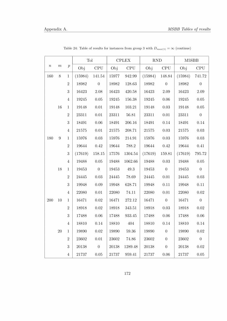
Appendix A. MSBB Tables of results
Table 24: Table of results for instances from group 3 with Dmax(1) = ∞ (continue)
Tol CPLEX RND M5SBBn m p
Obj CPU Obj CPU Obj CPU Obj CPU
160 8 1 (15984) 141.54 15977 942.99 (15984) 148.84 (15984) 741.72
2 18982 0 18982 128.63 18982 0 18982 0
3 16423 2.08 16423 420.58 16423 2.09 16423 2.09
4 19245 0.05 19245 156.38 19245 0.06 19245 0.05
16 1 19148 0.01 19148 103.21 19148 0.03 19148 0.05
2 23311 0.01 23311 56.81 23311 0.01 23311 0
3 18491 0.06 18491 206.16 18491 0.14 18491 0.14
4 21575 0.01 21575 208.71 21575 0.03 21575 0.03
180 9 1 15976 0.03 15976 214.91 15976 0.03 15976 0.03
2 19644 0.42 19644 788.2 19644 0.42 19644 0.41
3 (17619) 158.15 17576 1304.54 (17619) 159.81 (17619) 795.72
4 19488 0.05 19488 1062.66 19488 0.03 19488 0.05
18 1 19453 0 19453 49.3 19453 0 19453 0
2 24445 0.03 24445 78.69 24445 0.01 24445 0.03
3 19948 0.09 19948 628.71 19948 0.11 19948 0.11
4 22080 0.01 22080 74.11 22080 0.01 22080 0.02
200 10 1 16471 0.02 16471 272.12 16471 0 16471 0
2 18918 0.02 18918 343.51 18918 0.03 18918 0.02
3 17488 0.06 17488 933.45 17488 0.06 17488 0.06
4 18810 0.14 18810 404 18810 0.14 18810 0.14
20 1 19890 0.02 19890 59.36 19890 0 19890 0.02
2 23602 0.01 23602 74.86 23602 0 23602 0
3 20138 0 20138 1289.48 20138 0 20138 0.02
4 21737 0.05 21737 959.41 21737 0.06 21737 0.05
172
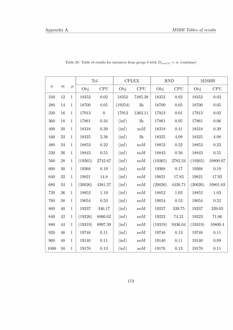
Appendix A. MSBB Tables of results
Table 25: Table of results for instances from group 3 with Dmax(1) = ∞ (continue)
Tol CPLEX RND M5SBBn m p
Obj CPU Obj CPU Obj CPU Obj CPU
240 12 1 18352 0.02 18352 7485.38 18352 0.02 18352 0.03
280 14 1 18700 0.05 (19254) 3h 18700 0.05 18700 0.05
320 16 1 17913 0 17913 1363.11 17913 0.01 17913 0.02
360 18 1 17861 0.34 (inf) 3h 17861 0.05 17861 0.06
400 20 1 18318 0.39 (inf) noM 18318 0.41 18318 0.39
440 22 1 18325 2.38 (inf) 3h 18325 4.09 18325 4.08
480 24 1 18853 0.22 (inf) noM 18853 0.22 18853 0.23
520 26 1 18843 0.55 (inf) noM 18843 0.56 18843 0.55
560 28 1 (19265) 2742.87 (inf) noM (19265) 2782.24 (19265) 10800.07
600 30 1 19368 0.19 (inf) noM 19368 0.17 19368 0.19
640 32 1 19821 14.8 (inf) noM 19821 17.83 19821 17.92
680 34 1 (20026) 4381.57 (inf) noM (20026) 4426.71 (20026) 10801.03
720 36 1 18852 1.19 (inf) noM 18852 1.03 18852 1.03
760 38 1 19054 0.53 (inf) noM 19054 0.53 19054 0.52
800 40 1 19237 346.17 (inf) noM 19237 339.75 19237 339.03
840 42 1 (19226) 8066.02 (inf) noM 19223 74.21 19223 71.66
880 44 1 (19319) 8997.39 (inf) noM (19319) 9436.04 (19319) 10800.4
920 46 1 19748 0.11 (inf) noM 19748 0.13 19748 0.11
960 48 1 19140 0.11 (inf) noM 19140 0.11 19140 0.09
1000 50 1 19176 0.13 (inf) noM 19176 0.13 19176 0.11
173
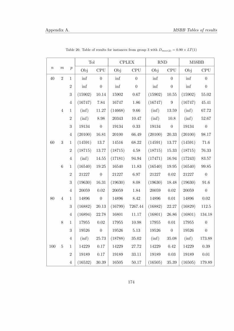
Appendix A. MSBB Tables of results
Table 26: Table of results for instances from group 3 with Dmax(2) = 0.90× LT (1)
Tol CPLEX RND M5SBBn m p
Obj CPU Obj CPU Obj CPU Obj CPU
40 2 1 inf 0 inf 0 inf 0 inf 0
2 inf 0 inf 0 inf 0 inf 0
3 (15902) 10.14 15902 0.67 (15902) 10.55 (15902) 55.02
4 (16747) 7.84 16747 1.86 (16747) 9 (16747) 45.41
4 1 (inf) 11.27 (14668) 9.66 (inf) 13.59 (inf) 67.72
2 (inf) 8.98 20343 10.47 (inf) 10.8 (inf) 52.67
3 19134 0 19134 0.33 19134 0 19134 0
4 (20100) 16.81 20100 66.49 (20100) 20.33 (20100) 98.17
60 3 1 (14591) 13.7 14516 68.22 (14591) 13.77 (14591) 71.6
2 (18715) 13.77 (18715) 4.58 (18715) 15.33 (18715) 76.33
4 (inf) 14.55 (17181) 94.94 (17471) 16.94 (17243) 83.57
6 1 (16540) 19.25 16540 11.83 (16540) 19.95 (16540) 99.85
2 21227 0 21227 6.97 21227 0.02 21227 0
3 (19630) 16.31 (19630) 8.08 (19630) 18.48 (19630) 91.6
4 20059 0.02 20059 1.84 20059 0.02 20059 0
80 4 1 14896 0 14896 8.42 14896 0.01 14896 0.02
3 (16882) 20.13 (16799) 7267.44 (16882) 22.27 (16829) 112.5
4 (16894) 22.78 16801 11.17 (16801) 26.86 (16801) 134.18
8 1 17955 0.02 17955 10.98 17955 0.01 17955 0
3 19526 0 19526 5.13 19526 0 19526 0
4 (inf) 25.73 (18788) 35.02 (inf) 35.08 (inf) 173.88
100 5 1 14229 0.17 14229 27.72 14229 0.42 14229 0.39
2 19189 0.17 19189 33.11 19189 0.03 19189 0.01
4 (16532) 30.39 16505 50.17 (16505) 35.39 (16505) 179.89
174
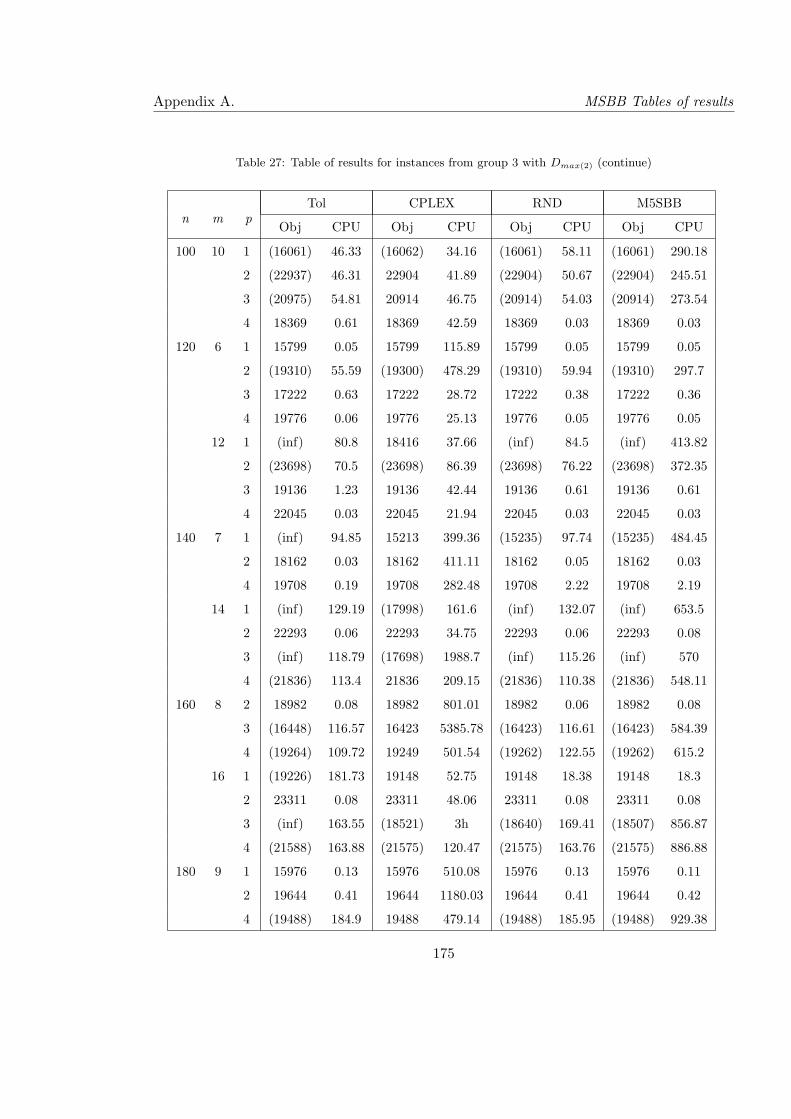
Appendix A. MSBB Tables of results
Table 27: Table of results for instances from group 3 with Dmax(2) (continue)
Tol CPLEX RND M5SBBn m p
Obj CPU Obj CPU Obj CPU Obj CPU
100 10 1 (16061) 46.33 (16062) 34.16 (16061) 58.11 (16061) 290.18
2 (22937) 46.31 22904 41.89 (22904) 50.67 (22904) 245.51
3 (20975) 54.81 20914 46.75 (20914) 54.03 (20914) 273.54
4 18369 0.61 18369 42.59 18369 0.03 18369 0.03
120 6 1 15799 0.05 15799 115.89 15799 0.05 15799 0.05
2 (19310) 55.59 (19300) 478.29 (19310) 59.94 (19310) 297.7
3 17222 0.63 17222 28.72 17222 0.38 17222 0.36
4 19776 0.06 19776 25.13 19776 0.05 19776 0.05
12 1 (inf) 80.8 18416 37.66 (inf) 84.5 (inf) 413.82
2 (23698) 70.5 (23698) 86.39 (23698) 76.22 (23698) 372.35
3 19136 1.23 19136 42.44 19136 0.61 19136 0.61
4 22045 0.03 22045 21.94 22045 0.03 22045 0.03
140 7 1 (inf) 94.85 15213 399.36 (15235) 97.74 (15235) 484.45
2 18162 0.03 18162 411.11 18162 0.05 18162 0.03
4 19708 0.19 19708 282.48 19708 2.22 19708 2.19
14 1 (inf) 129.19 (17998) 161.6 (inf) 132.07 (inf) 653.5
2 22293 0.06 22293 34.75 22293 0.06 22293 0.08
3 (inf) 118.79 (17698) 1988.7 (inf) 115.26 (inf) 570
4 (21836) 113.4 21836 209.15 (21836) 110.38 (21836) 548.11
160 8 2 18982 0.08 18982 801.01 18982 0.06 18982 0.08
3 (16448) 116.57 16423 5385.78 (16423) 116.61 (16423) 584.39
4 (19264) 109.72 19249 501.54 (19262) 122.55 (19262) 615.2
16 1 (19226) 181.73 19148 52.75 19148 18.38 19148 18.3
2 23311 0.08 23311 48.06 23311 0.08 23311 0.08
3 (inf) 163.55 (18521) 3h (18640) 169.41 (18507) 856.87
4 (21588) 163.88 (21575) 120.47 (21575) 163.76 (21575) 886.88
180 9 1 15976 0.13 15976 510.08 15976 0.13 15976 0.11
2 19644 0.41 19644 1180.03 19644 0.41 19644 0.42
4 (19488) 184.9 19488 479.14 (19488) 185.95 (19488) 929.38
175
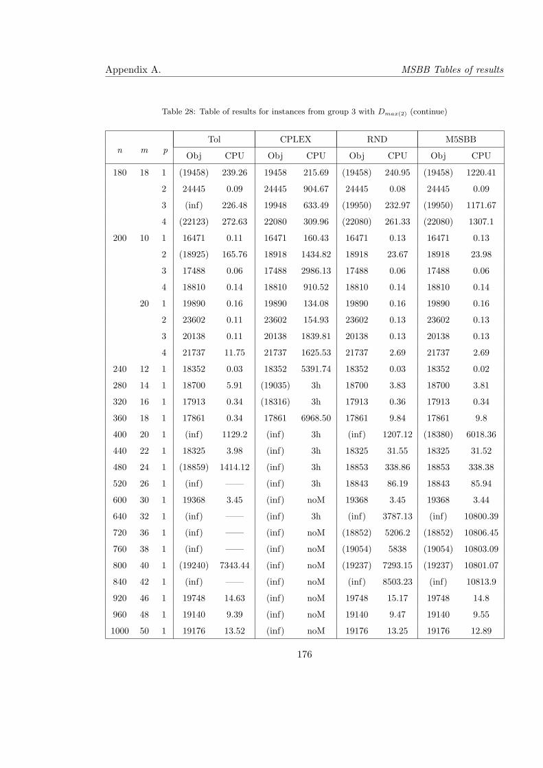
Appendix A. MSBB Tables of results
Table 28: Table of results for instances from group 3 with Dmax(2) (continue)
Tol CPLEX RND M5SBBn m p
Obj CPU Obj CPU Obj CPU Obj CPU
180 18 1 (19458) 239.26 19458 215.69 (19458) 240.95 (19458) 1220.41
2 24445 0.09 24445 904.67 24445 0.08 24445 0.09
3 (inf) 226.48 19948 633.49 (19950) 232.97 (19950) 1171.67
4 (22123) 272.63 22080 309.96 (22080) 261.33 (22080) 1307.1
200 10 1 16471 0.11 16471 160.43 16471 0.13 16471 0.13
2 (18925) 165.76 18918 1434.82 18918 23.67 18918 23.98
3 17488 0.06 17488 2986.13 17488 0.06 17488 0.06
4 18810 0.14 18810 910.52 18810 0.14 18810 0.14
20 1 19890 0.16 19890 134.08 19890 0.16 19890 0.16
2 23602 0.11 23602 154.93 23602 0.13 23602 0.13
3 20138 0.11 20138 1839.81 20138 0.13 20138 0.13
4 21737 11.75 21737 1625.53 21737 2.69 21737 2.69
240 12 1 18352 0.03 18352 5391.74 18352 0.03 18352 0.02
280 14 1 18700 5.91 (19035) 3h 18700 3.83 18700 3.81
320 16 1 17913 0.34 (18316) 3h 17913 0.36 17913 0.34
360 18 1 17861 0.34 17861 6968.50 17861 9.84 17861 9.8
400 20 1 (inf) 1129.2 (inf) 3h (inf) 1207.12 (18380) 6018.36
440 22 1 18325 3.98 (inf) 3h 18325 31.55 18325 31.52
480 24 1 (18859) 1414.12 (inf) 3h 18853 338.86 18853 338.38
520 26 1 (inf) —— (inf) 3h 18843 86.19 18843 85.94
600 30 1 19368 3.45 (inf) noM 19368 3.45 19368 3.44
640 32 1 (inf) —— (inf) 3h (inf) 3787.13 (inf) 10800.39
720 36 1 (inf) —— (inf) noM (18852) 5206.2 (18852) 10806.45
760 38 1 (inf) —— (inf) noM (19054) 5838 (19054) 10803.09
800 40 1 (19240) 7343.44 (inf) noM (19237) 7293.15 (19237) 10801.07
840 42 1 (inf) —— (inf) noM (inf) 8503.23 (inf) 10813.9
920 46 1 19748 14.63 (inf) noM 19748 15.17 19748 14.8
960 48 1 19140 9.39 (inf) noM 19140 9.47 19140 9.55
1000 50 1 19176 13.52 (inf) noM 19176 13.25 19176 12.89
176
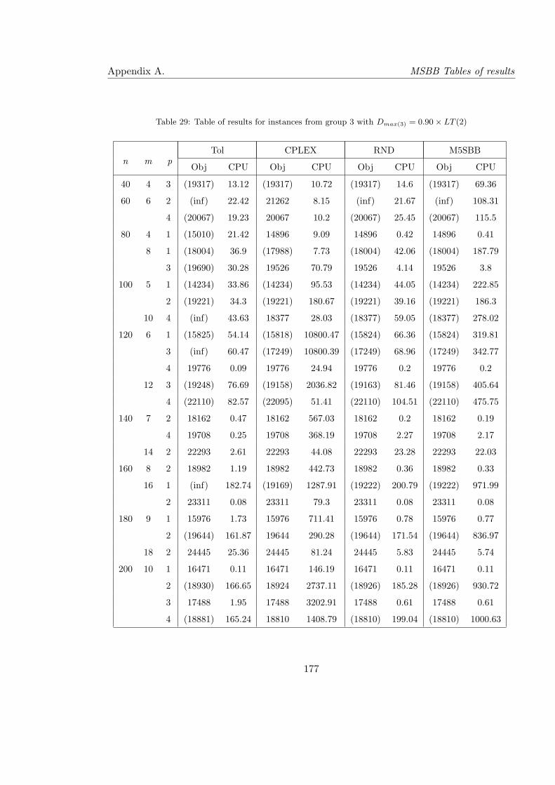
Appendix A. MSBB Tables of results
Table 29: Table of results for instances from group 3 with Dmax(3) = 0.90× LT (2)
Tol CPLEX RND M5SBBn m p
Obj CPU Obj CPU Obj CPU Obj CPU
40 4 3 (19317) 13.12 (19317) 10.72 (19317) 14.6 (19317) 69.36
60 6 2 (inf) 22.42 21262 8.15 (inf) 21.67 (inf) 108.31
4 (20067) 19.23 20067 10.2 (20067) 25.45 (20067) 115.5
80 4 1 (15010) 21.42 14896 9.09 14896 0.42 14896 0.41
8 1 (18004) 36.9 (17988) 7.73 (18004) 42.06 (18004) 187.79
3 (19690) 30.28 19526 70.79 19526 4.14 19526 3.8
100 5 1 (14234) 33.86 (14234) 95.53 (14234) 44.05 (14234) 222.85
2 (19221) 34.3 (19221) 180.67 (19221) 39.16 (19221) 186.3
10 4 (inf) 43.63 18377 28.03 (18377) 59.05 (18377) 278.02
120 6 1 (15825) 54.14 (15818) 10800.47 (15824) 66.36 (15824) 319.81
3 (inf) 60.47 (17249) 10800.39 (17249) 68.96 (17249) 342.77
4 19776 0.09 19776 24.94 19776 0.2 19776 0.2
12 3 (19248) 76.69 (19158) 2036.82 (19163) 81.46 (19158) 405.64
4 (22110) 82.57 (22095) 51.41 (22110) 104.51 (22110) 475.75
140 7 2 18162 0.47 18162 567.03 18162 0.2 18162 0.19
4 19708 0.25 19708 368.19 19708 2.27 19708 2.17
14 2 22293 2.61 22293 44.08 22293 23.28 22293 22.03
160 8 2 18982 1.19 18982 442.73 18982 0.36 18982 0.33
16 1 (inf) 182.74 (19169) 1287.91 (19222) 200.79 (19222) 971.99
2 23311 0.08 23311 79.3 23311 0.08 23311 0.08
180 9 1 15976 1.73 15976 711.41 15976 0.78 15976 0.77
2 (19644) 161.87 19644 290.28 (19644) 171.54 (19644) 836.97
18 2 24445 25.36 24445 81.24 24445 5.83 24445 5.74
200 10 1 16471 0.11 16471 146.19 16471 0.11 16471 0.11
2 (18930) 166.65 18924 2737.11 (18926) 185.28 (18926) 930.72
3 17488 1.95 17488 3202.91 17488 0.61 17488 0.61
4 (18881) 165.24 18810 1408.79 (18810) 199.04 (18810) 1000.63
177
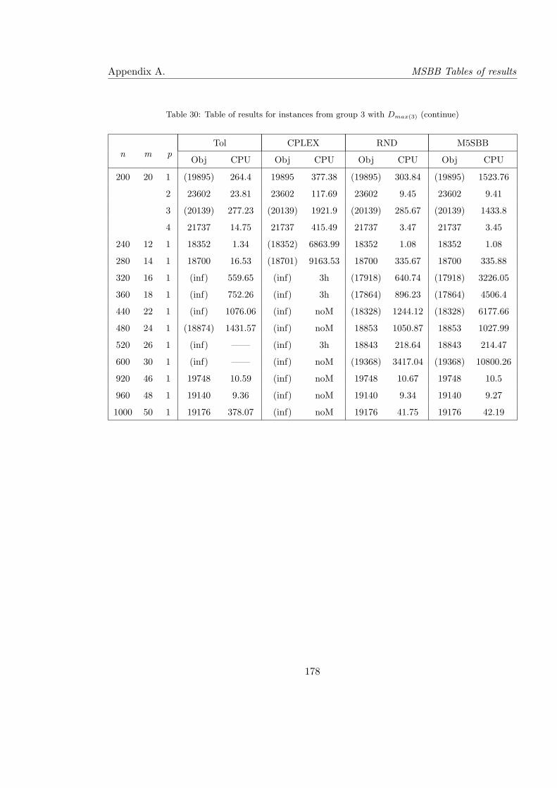
Appendix A. MSBB Tables of results
Table 30: Table of results for instances from group 3 with Dmax(3) (continue)
Tol CPLEX RND M5SBBn m p
Obj CPU Obj CPU Obj CPU Obj CPU
200 20 1 (19895) 264.4 19895 377.38 (19895) 303.84 (19895) 1523.76
2 23602 23.81 23602 117.69 23602 9.45 23602 9.41
3 (20139) 277.23 (20139) 1921.9 (20139) 285.67 (20139) 1433.8
4 21737 14.75 21737 415.49 21737 3.47 21737 3.45
240 12 1 18352 1.34 (18352) 6863.99 18352 1.08 18352 1.08
280 14 1 18700 16.53 (18701) 9163.53 18700 335.67 18700 335.88
320 16 1 (inf) 559.65 (inf) 3h (17918) 640.74 (17918) 3226.05
360 18 1 (inf) 752.26 (inf) 3h (17864) 896.23 (17864) 4506.4
440 22 1 (inf) 1076.06 (inf) noM (18328) 1244.12 (18328) 6177.66
480 24 1 (18874) 1431.57 (inf) noM 18853 1050.87 18853 1027.99
520 26 1 (inf) —— (inf) 3h 18843 218.64 18843 214.47
600 30 1 (inf) —— (inf) noM (19368) 3417.04 (19368) 10800.26
920 46 1 19748 10.59 (inf) noM 19748 10.67 19748 10.5
960 48 1 19140 9.36 (inf) noM 19140 9.34 19140 9.27
1000 50 1 19176 378.07 (inf) noM 19176 41.75 19176 42.19
178
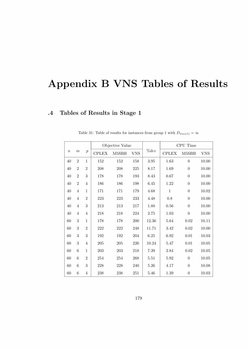
Appendix B VNS Tables of Results
.4 Tables of Results in Stage 1
Table 31: Table of results for instances from group 1 with Dmax(1) = ∞
Objective Value CPU Timen m p
CPLEX M5SBB VNS%dev
CPLEX M5SBB VNS
40 2 1 152 152 158 3.95 1.63 0 10.00
40 2 2 208 208 225 8.17 1.69 0 10.00
40 2 3 178 178 193 8.43 0.67 0 10.00
40 2 4 186 186 198 6.45 1.22 0 10.00
40 4 1 171 171 179 4.68 1 0 10.02
40 4 2 223 223 233 4.48 0.8 0 10.00
40 4 3 213 213 217 1.88 0.56 0 10.00
40 4 4 218 218 224 2.75 1.03 0 10.00
60 3 1 178 178 200 12.36 5.64 0.02 10.11
60 3 2 222 222 248 11.71 3.42 0.02 10.00
60 3 3 192 192 204 6.25 6.92 0.01 10.03
60 3 4 205 205 226 10.24 5.47 0.01 10.05
60 6 1 203 203 218 7.39 2.84 0.02 10.05
60 6 2 254 254 268 5.51 5.92 0 10.05
60 6 3 228 228 240 5.26 4.17 0 10.08
60 6 4 238 238 251 5.46 1.39 0 10.03
179
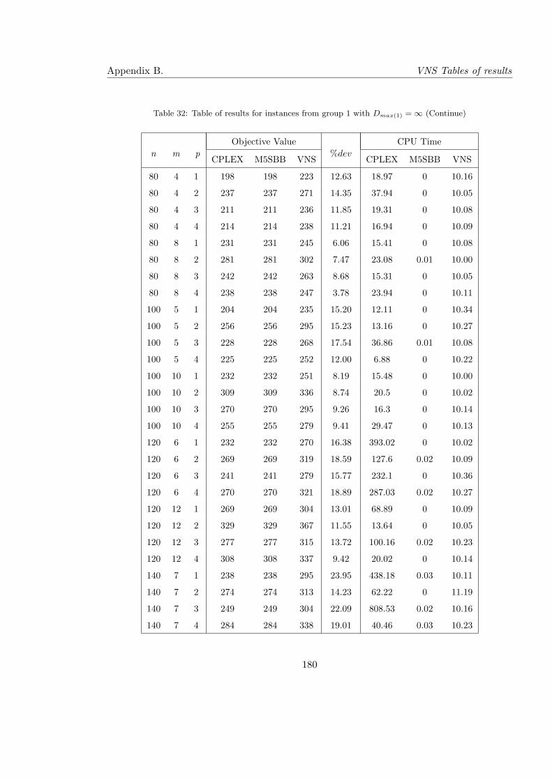
Appendix B. VNS Tables of results
Table 32: Table of results for instances from group 1 with Dmax(1) = ∞ (Continue)
Objective Value CPU Timen m p
CPLEX M5SBB VNS%dev
CPLEX M5SBB VNS
80 4 1 198 198 223 12.63 18.97 0 10.16
80 4 2 237 237 271 14.35 37.94 0 10.05
80 4 3 211 211 236 11.85 19.31 0 10.08
80 4 4 214 214 238 11.21 16.94 0 10.09
80 8 1 231 231 245 6.06 15.41 0 10.08
80 8 2 281 281 302 7.47 23.08 0.01 10.00
80 8 3 242 242 263 8.68 15.31 0 10.05
80 8 4 238 238 247 3.78 23.94 0 10.11
100 5 1 204 204 235 15.20 12.11 0 10.34
100 5 2 256 256 295 15.23 13.16 0 10.27
100 5 3 228 228 268 17.54 36.86 0.01 10.08
100 5 4 225 225 252 12.00 6.88 0 10.22
100 10 1 232 232 251 8.19 15.48 0 10.00
100 10 2 309 309 336 8.74 20.5 0 10.02
100 10 3 270 270 295 9.26 16.3 0 10.14
100 10 4 255 255 279 9.41 29.47 0 10.13
120 6 1 232 232 270 16.38 393.02 0 10.02
120 6 2 269 269 319 18.59 127.6 0.02 10.09
120 6 3 241 241 279 15.77 232.1 0 10.36
120 6 4 270 270 321 18.89 287.03 0.02 10.27
120 12 1 269 269 304 13.01 68.89 0 10.09
120 12 2 329 329 367 11.55 13.64 0 10.05
120 12 3 277 277 315 13.72 100.16 0.02 10.23
120 12 4 308 308 337 9.42 20.02 0 10.14
140 7 1 238 238 295 23.95 438.18 0.03 10.11
140 7 2 274 274 313 14.23 62.22 0 11.19
140 7 3 249 249 304 22.09 808.53 0.02 10.16
140 7 4 284 284 338 19.01 40.46 0.03 10.23
180
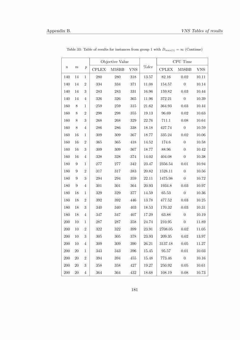
Appendix B. VNS Tables of results
Table 33: Table of results for instances from group 1 with Dmax(1) = ∞ (Continue)
Objective Value CPU Timen m p
CPLEX M5SBB VNS%dev
CPLEX M5SBB VNS
140 14 1 280 280 318 13.57 82.16 0.02 10.11
140 14 2 334 334 371 11.08 154.57 0 10.14
140 14 3 283 283 331 16.96 159.82 0.03 10.44
140 14 4 326 326 365 11.96 372.21 0 10.39
160 8 1 259 259 315 21.62 364.93 0.03 10.44
160 8 2 298 298 355 19.13 96.69 0.02 10.63
160 8 3 268 268 329 22.76 711.1 0.08 10.64
160 8 4 286 286 338 18.18 427.74 0 10.59
160 16 1 309 309 367 18.77 335.24 0.02 10.06
160 16 2 365 365 418 14.52 174.6 0 10.58
160 16 3 309 309 367 18.77 88.96 0 10.42
160 16 4 328 328 374 14.02 404.08 0 10.38
180 9 1 277 277 342 23.47 2356.54 0.01 10.94
180 9 2 317 317 383 20.82 1528.11 0 10.56
180 9 3 294 294 359 22.11 1475.98 0 10.72
180 9 4 301 301 364 20.93 1934.8 0.03 10.97
180 18 1 329 329 377 14.59 65.53 0 10.36
180 18 2 392 392 446 13.78 477.52 0.03 10.25
180 18 3 340 340 403 18.53 170.32 0.03 10.31
180 18 4 347 347 407 17.29 63.88 0 10.19
200 10 1 287 287 358 24.74 210.95 0 11.89
200 10 2 322 322 399 23.91 2708.05 0.02 11.05
200 10 3 305 305 378 23.93 209.35 0.02 13.97
200 10 4 309 309 390 26.21 3137.18 0.05 11.27
200 20 1 343 343 396 15.45 95.57 0.01 10.03
200 20 2 394 394 455 15.48 773.46 0 10.16
200 20 3 358 358 427 19.27 250.92 0.05 10.61
200 20 4 364 364 432 18.68 108.19 0.08 10.73
181
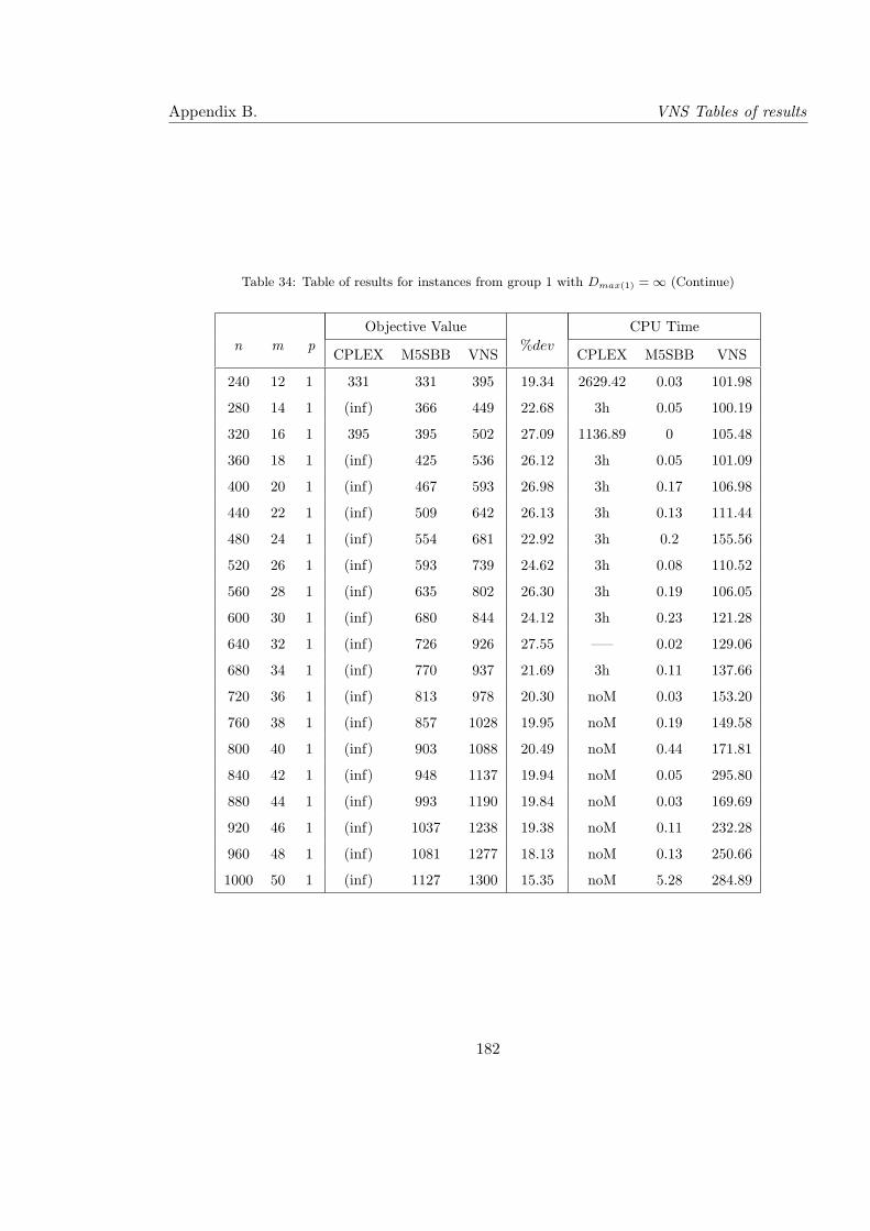
Appendix B. VNS Tables of results
Table 34: Table of results for instances from group 1 with Dmax(1) = ∞ (Continue)
Objective Value CPU Timen m p
CPLEX M5SBB VNS%dev
CPLEX M5SBB VNS
240 12 1 331 331 395 19.34 2629.42 0.03 101.98
280 14 1 (inf) 366 449 22.68 3h 0.05 100.19
320 16 1 395 395 502 27.09 1136.89 0 105.48
360 18 1 (inf) 425 536 26.12 3h 0.05 101.09
400 20 1 (inf) 467 593 26.98 3h 0.17 106.98
440 22 1 (inf) 509 642 26.13 3h 0.13 111.44
480 24 1 (inf) 554 681 22.92 3h 0.2 155.56
520 26 1 (inf) 593 739 24.62 3h 0.08 110.52
560 28 1 (inf) 635 802 26.30 3h 0.19 106.05
600 30 1 (inf) 680 844 24.12 3h 0.23 121.28
640 32 1 (inf) 726 926 27.55 —– 0.02 129.06
680 34 1 (inf) 770 937 21.69 3h 0.11 137.66
720 36 1 (inf) 813 978 20.30 noM 0.03 153.20
760 38 1 (inf) 857 1028 19.95 noM 0.19 149.58
800 40 1 (inf) 903 1088 20.49 noM 0.44 171.81
840 42 1 (inf) 948 1137 19.94 noM 0.05 295.80
880 44 1 (inf) 993 1190 19.84 noM 0.03 169.69
920 46 1 (inf) 1037 1238 19.38 noM 0.11 232.28
960 48 1 (inf) 1081 1277 18.13 noM 0.13 250.66
1000 50 1 (inf) 1127 1300 15.35 noM 5.28 284.89
182
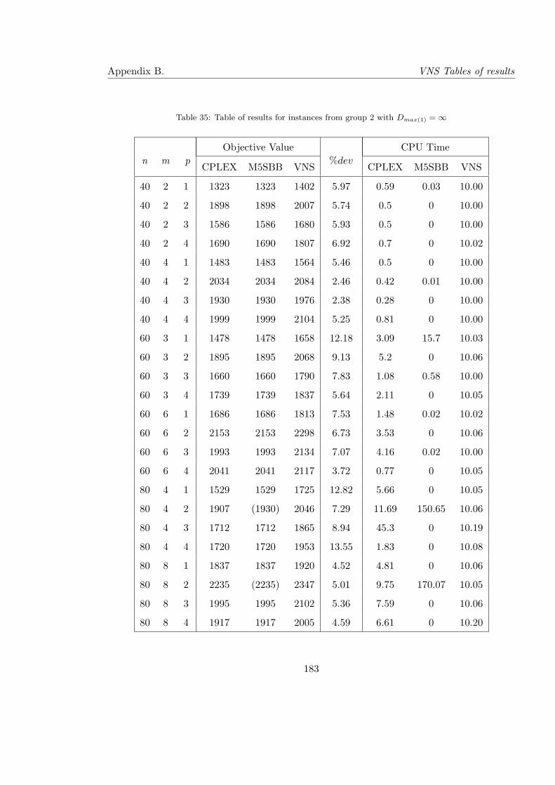
Appendix B. VNS Tables of results
Table 35: Table of results for instances from group 2 with Dmax(1) = ∞
Objective Value CPU Timen m p
CPLEX M5SBB VNS%dev
CPLEX M5SBB VNS
40 2 1 1323 1323 1402 5.97 0.59 0.03 10.00
40 2 2 1898 1898 2007 5.74 0.5 0 10.00
40 2 3 1586 1586 1680 5.93 0.5 0 10.00
40 2 4 1690 1690 1807 6.92 0.7 0 10.02
40 4 1 1483 1483 1564 5.46 0.5 0 10.00
40 4 2 2034 2034 2084 2.46 0.42 0.01 10.00
40 4 3 1930 1930 1976 2.38 0.28 0 10.00
40 4 4 1999 1999 2104 5.25 0.81 0 10.00
60 3 1 1478 1478 1658 12.18 3.09 15.7 10.03
60 3 2 1895 1895 2068 9.13 5.2 0 10.06
60 3 3 1660 1660 1790 7.83 1.08 0.58 10.00
60 3 4 1739 1739 1837 5.64 2.11 0 10.05
60 6 1 1686 1686 1813 7.53 1.48 0.02 10.02
60 6 2 2153 2153 2298 6.73 3.53 0 10.06
60 6 3 1993 1993 2134 7.07 4.16 0.02 10.00
60 6 4 2041 2041 2117 3.72 0.77 0 10.05
80 4 1 1529 1529 1725 12.82 5.66 0 10.05
80 4 2 1907 (1930) 2046 7.29 11.69 150.65 10.06
80 4 3 1712 1712 1865 8.94 45.3 0 10.19
80 4 4 1720 1720 1953 13.55 1.83 0 10.08
80 8 1 1837 1837 1920 4.52 4.81 0 10.06
80 8 2 2235 (2235) 2347 5.01 9.75 170.07 10.05
80 8 3 1995 1995 2102 5.36 7.59 0 10.06
80 8 4 1917 1917 2005 4.59 6.61 0 10.20
183
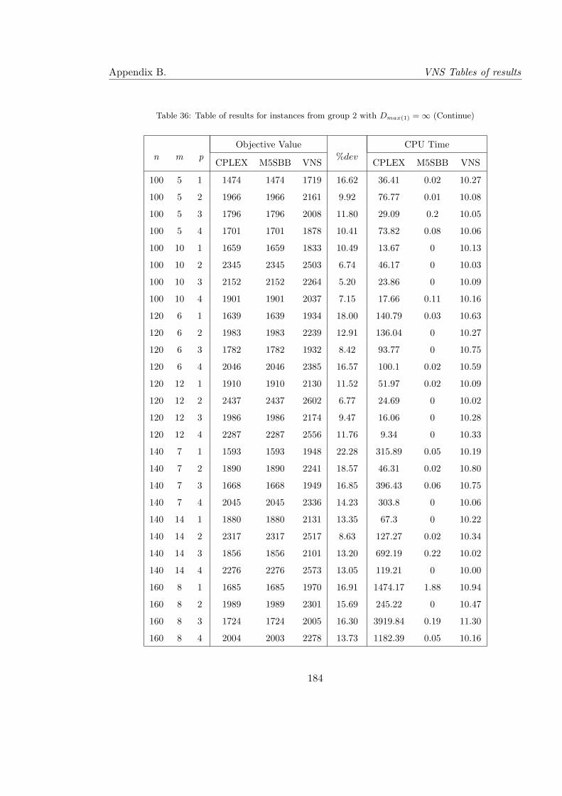
Appendix B. VNS Tables of results
Table 36: Table of results for instances from group 2 with Dmax(1) = ∞ (Continue)
Objective Value CPU Timen m p
CPLEX M5SBB VNS%dev
CPLEX M5SBB VNS
100 5 1 1474 1474 1719 16.62 36.41 0.02 10.27
100 5 2 1966 1966 2161 9.92 76.77 0.01 10.08
100 5 3 1796 1796 2008 11.80 29.09 0.2 10.05
100 5 4 1701 1701 1878 10.41 73.82 0.08 10.06
100 10 1 1659 1659 1833 10.49 13.67 0 10.13
100 10 2 2345 2345 2503 6.74 46.17 0 10.03
100 10 3 2152 2152 2264 5.20 23.86 0 10.09
100 10 4 1901 1901 2037 7.15 17.66 0.11 10.16
120 6 1 1639 1639 1934 18.00 140.79 0.03 10.63
120 6 2 1983 1983 2239 12.91 136.04 0 10.27
120 6 3 1782 1782 1932 8.42 93.77 0 10.75
120 6 4 2046 2046 2385 16.57 100.1 0.02 10.59
120 12 1 1910 1910 2130 11.52 51.97 0.02 10.09
120 12 2 2437 2437 2602 6.77 24.69 0 10.02
120 12 3 1986 1986 2174 9.47 16.06 0 10.28
120 12 4 2287 2287 2556 11.76 9.34 0 10.33
140 7 1 1593 1593 1948 22.28 315.89 0.05 10.19
140 7 2 1890 1890 2241 18.57 46.31 0.02 10.80
140 7 3 1668 1668 1949 16.85 396.43 0.06 10.75
140 7 4 2045 2045 2336 14.23 303.8 0 10.06
140 14 1 1880 1880 2131 13.35 67.3 0 10.22
140 14 2 2317 2317 2517 8.63 127.27 0.02 10.34
140 14 3 1856 1856 2101 13.20 692.19 0.22 10.02
140 14 4 2276 2276 2573 13.05 119.21 0 10.00
160 8 1 1685 1685 1970 16.91 1474.17 1.88 10.94
160 8 2 1989 1989 2301 15.69 245.22 0 10.47
160 8 3 1724 1724 2005 16.30 3919.84 0.19 11.30
160 8 4 2004 2003 2278 13.73 1182.39 0.05 10.16
184
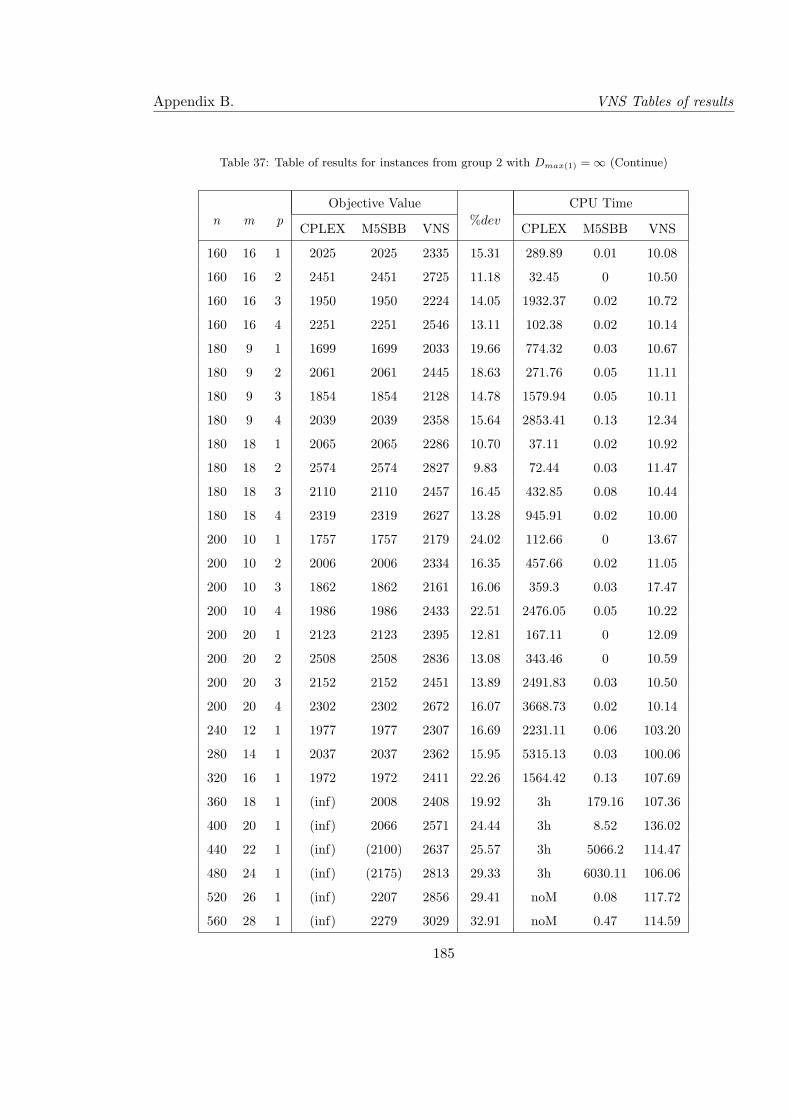
Appendix B. VNS Tables of results
Table 37: Table of results for instances from group 2 with Dmax(1) = ∞ (Continue)
Objective Value CPU Timen m p
CPLEX M5SBB VNS%dev
CPLEX M5SBB VNS
160 16 1 2025 2025 2335 15.31 289.89 0.01 10.08
160 16 2 2451 2451 2725 11.18 32.45 0 10.50
160 16 3 1950 1950 2224 14.05 1932.37 0.02 10.72
160 16 4 2251 2251 2546 13.11 102.38 0.02 10.14
180 9 1 1699 1699 2033 19.66 774.32 0.03 10.67
180 9 2 2061 2061 2445 18.63 271.76 0.05 11.11
180 9 3 1854 1854 2128 14.78 1579.94 0.05 10.11
180 9 4 2039 2039 2358 15.64 2853.41 0.13 12.34
180 18 1 2065 2065 2286 10.70 37.11 0.02 10.92
180 18 2 2574 2574 2827 9.83 72.44 0.03 11.47
180 18 3 2110 2110 2457 16.45 432.85 0.08 10.44
180 18 4 2319 2319 2627 13.28 945.91 0.02 10.00
200 10 1 1757 1757 2179 24.02 112.66 0 13.67
200 10 2 2006 2006 2334 16.35 457.66 0.02 11.05
200 10 3 1862 1862 2161 16.06 359.3 0.03 17.47
200 10 4 1986 1986 2433 22.51 2476.05 0.05 10.22
200 20 1 2123 2123 2395 12.81 167.11 0 12.09
200 20 2 2508 2508 2836 13.08 343.46 0 10.59
200 20 3 2152 2152 2451 13.89 2491.83 0.03 10.50
200 20 4 2302 2302 2672 16.07 3668.73 0.02 10.14
240 12 1 1977 1977 2307 16.69 2231.11 0.06 103.20
280 14 1 2037 2037 2362 15.95 5315.13 0.03 100.06
320 16 1 1972 1972 2411 22.26 1564.42 0.13 107.69
360 18 1 (inf) 2008 2408 19.92 3h 179.16 107.36
400 20 1 (inf) 2066 2571 24.44 3h 8.52 136.02
440 22 1 (inf) (2100) 2637 25.57 3h 5066.2 114.47
480 24 1 (inf) (2175) 2813 29.33 3h 6030.11 106.06
520 26 1 (inf) 2207 2856 29.41 noM 0.08 117.72
560 28 1 (inf) 2279 3029 32.91 noM 0.47 114.59
185

Appendix B. VNS Tables of results
Table 38: Table of results for instances from group 2 with Dmax(1) = ∞ (Continue)
Objective Value CPU Timen m p
CPLEX M5SBB VNS%dev
CPLEX M5SBB VNS
600 30 1 (inf) (2309) 2999 29.88 noM 9656.18 155.78
640 32 1 (inf) 2395 3125 30.48 noM 0.39 151.50
680 34 1 (inf) 2437 3238 32.87 noM 23.09 150.52
720 36 1 (inf) 2365 3154 33.36 noM 0.19 192.47
760 38 1 (inf) (2411) 3333 38.24 noM 10800.19 169.75
800 40 1 (inf) (2452) 3239 32.10 noM 10800.18 284.00
840 42 1 (inf) 2470 3320 34.41 noM 0.89 374.00
880 44 1 (inf) 2513 3361 33.74 noM 2.2 324.47
920 46 1 (inf) 2578 3549 37.66 noM 3.73 329.17
960 48 1 (inf) 2577 3450 33.88 noM 4.73 632.05
1000 50 1 (inf) 2614 3589 37.30 noM 0.42 311.13
186
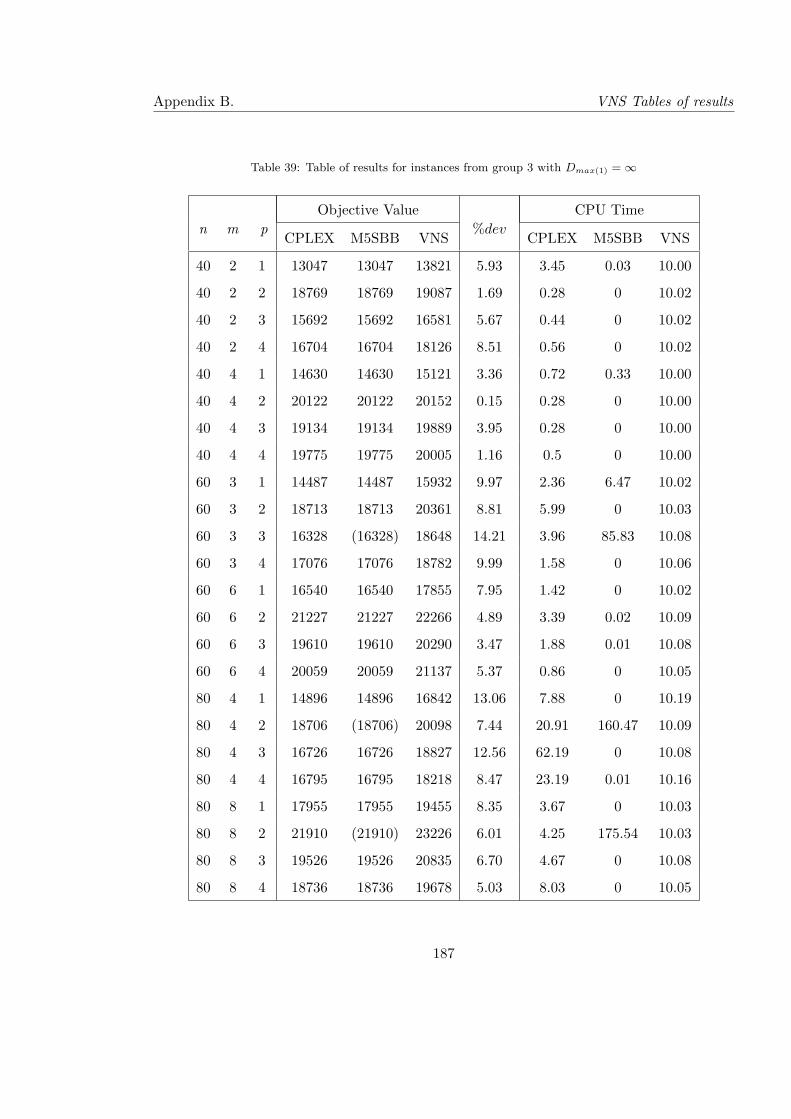
Appendix B. VNS Tables of results
Table 39: Table of results for instances from group 3 with Dmax(1) = ∞
Objective Value CPU Timen m p
CPLEX M5SBB VNS%dev
CPLEX M5SBB VNS
40 2 1 13047 13047 13821 5.93 3.45 0.03 10.00
40 2 2 18769 18769 19087 1.69 0.28 0 10.02
40 2 3 15692 15692 16581 5.67 0.44 0 10.02
40 2 4 16704 16704 18126 8.51 0.56 0 10.02
40 4 1 14630 14630 15121 3.36 0.72 0.33 10.00
40 4 2 20122 20122 20152 0.15 0.28 0 10.00
40 4 3 19134 19134 19889 3.95 0.28 0 10.00
40 4 4 19775 19775 20005 1.16 0.5 0 10.00
60 3 1 14487 14487 15932 9.97 2.36 6.47 10.02
60 3 2 18713 18713 20361 8.81 5.99 0 10.03
60 3 3 16328 (16328) 18648 14.21 3.96 85.83 10.08
60 3 4 17076 17076 18782 9.99 1.58 0 10.06
60 6 1 16540 16540 17855 7.95 1.42 0 10.02
60 6 2 21227 21227 22266 4.89 3.39 0.02 10.09
60 6 3 19610 19610 20290 3.47 1.88 0.01 10.08
60 6 4 20059 20059 21137 5.37 0.86 0 10.05
80 4 1 14896 14896 16842 13.06 7.88 0 10.19
80 4 2 18706 (18706) 20098 7.44 20.91 160.47 10.09
80 4 3 16726 16726 18827 12.56 62.19 0 10.08
80 4 4 16795 16795 18218 8.47 23.19 0.01 10.16
80 8 1 17955 17955 19455 8.35 3.67 0 10.03
80 8 2 21910 (21910) 23226 6.01 4.25 175.54 10.03
80 8 3 19526 19526 20835 6.70 4.67 0 10.08
80 8 4 18736 18736 19678 5.03 8.03 0 10.05
187
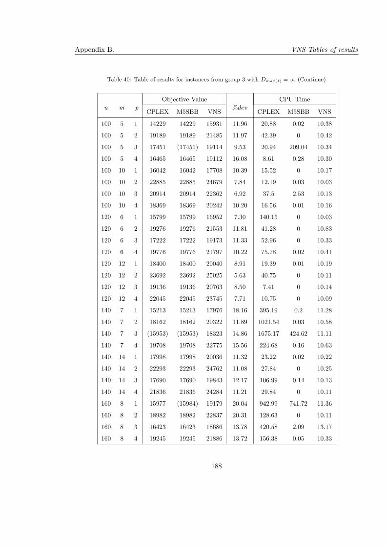
Appendix B. VNS Tables of results
Table 40: Table of results for instances from group 3 with Dmax(1) = ∞ (Continue)
Objective Value CPU Timen m p
CPLEX M5SBB VNS%dev
CPLEX M5SBB VNS
100 5 1 14229 14229 15931 11.96 20.88 0.02 10.38
100 5 2 19189 19189 21485 11.97 42.39 0 10.42
100 5 3 17451 (17451) 19114 9.53 20.94 209.04 10.34
100 5 4 16465 16465 19112 16.08 8.61 0.28 10.30
100 10 1 16042 16042 17708 10.39 15.52 0 10.17
100 10 2 22885 22885 24679 7.84 12.19 0.03 10.03
100 10 3 20914 20914 22362 6.92 37.5 2.53 10.13
100 10 4 18369 18369 20242 10.20 16.56 0.01 10.16
120 6 1 15799 15799 16952 7.30 140.15 0 10.03
120 6 2 19276 19276 21553 11.81 41.28 0 10.83
120 6 3 17222 17222 19173 11.33 52.96 0 10.33
120 6 4 19776 19776 21797 10.22 75.78 0.02 10.41
120 12 1 18400 18400 20040 8.91 19.39 0.01 10.19
120 12 2 23692 23692 25025 5.63 40.75 0 10.11
120 12 3 19136 19136 20763 8.50 7.41 0 10.14
120 12 4 22045 22045 23745 7.71 10.75 0 10.09
140 7 1 15213 15213 17976 18.16 395.19 0.2 11.28
140 7 2 18162 18162 20322 11.89 1021.54 0.03 10.58
140 7 3 (15953) (15953) 18323 14.86 1675.17 424.62 11.11
140 7 4 19708 19708 22775 15.56 224.68 0.16 10.63
140 14 1 17998 17998 20036 11.32 23.22 0.02 10.22
140 14 2 22293 22293 24762 11.08 27.84 0 10.25
140 14 3 17690 17690 19843 12.17 106.99 0.14 10.13
140 14 4 21836 21836 24284 11.21 29.84 0 10.11
160 8 1 15977 (15984) 19179 20.04 942.99 741.72 11.36
160 8 2 18982 18982 22837 20.31 128.63 0 10.11
160 8 3 16423 16423 18686 13.78 420.58 2.09 13.17
160 8 4 19245 19245 21886 13.72 156.38 0.05 10.33
188
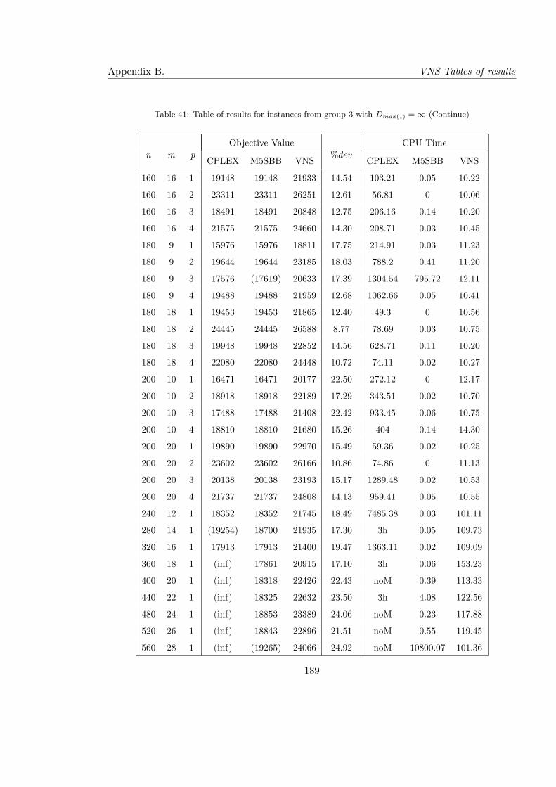
Appendix B. VNS Tables of results
Table 41: Table of results for instances from group 3 with Dmax(1) = ∞ (Continue)
Objective Value CPU Timen m p
CPLEX M5SBB VNS%dev
CPLEX M5SBB VNS
160 16 1 19148 19148 21933 14.54 103.21 0.05 10.22
160 16 2 23311 23311 26251 12.61 56.81 0 10.06
160 16 3 18491 18491 20848 12.75 206.16 0.14 10.20
160 16 4 21575 21575 24660 14.30 208.71 0.03 10.45
180 9 1 15976 15976 18811 17.75 214.91 0.03 11.23
180 9 2 19644 19644 23185 18.03 788.2 0.41 11.20
180 9 3 17576 (17619) 20633 17.39 1304.54 795.72 12.11
180 9 4 19488 19488 21959 12.68 1062.66 0.05 10.41
180 18 1 19453 19453 21865 12.40 49.3 0 10.56
180 18 2 24445 24445 26588 8.77 78.69 0.03 10.75
180 18 3 19948 19948 22852 14.56 628.71 0.11 10.20
180 18 4 22080 22080 24448 10.72 74.11 0.02 10.27
200 10 1 16471 16471 20177 22.50 272.12 0 12.17
200 10 2 18918 18918 22189 17.29 343.51 0.02 10.70
200 10 3 17488 17488 21408 22.42 933.45 0.06 10.75
200 10 4 18810 18810 21680 15.26 404 0.14 14.30
200 20 1 19890 19890 22970 15.49 59.36 0.02 10.25
200 20 2 23602 23602 26166 10.86 74.86 0 11.13
200 20 3 20138 20138 23193 15.17 1289.48 0.02 10.53
200 20 4 21737 21737 24808 14.13 959.41 0.05 10.55
240 12 1 18352 18352 21745 18.49 7485.38 0.03 101.11
280 14 1 (19254) 18700 21935 17.30 3h 0.05 109.73
320 16 1 17913 17913 21400 19.47 1363.11 0.02 109.09
360 18 1 (inf) 17861 20915 17.10 3h 0.06 153.23
400 20 1 (inf) 18318 22426 22.43 noM 0.39 113.33
440 22 1 (inf) 18325 22632 23.50 3h 4.08 122.56
480 24 1 (inf) 18853 23389 24.06 noM 0.23 117.88
520 26 1 (inf) 18843 22896 21.51 noM 0.55 119.45
560 28 1 (inf) (19265) 24066 24.92 noM 10800.07 101.36
189
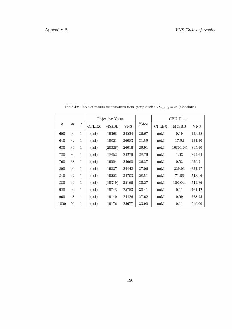
Appendix B. VNS Tables of results
Table 42: Table of results for instances from group 3 with Dmax(1) = ∞ (Continue)
Objective Value CPU Timen m p
CPLEX M5SBB VNS%dev
CPLEX M5SBB VNS
600 30 1 (inf) 19368 24534 26.67 noM 0.19 133.38
640 32 1 (inf) 19821 26083 31.59 noM 17.92 131.50
680 34 1 (inf) (20026) 26016 29.91 noM 10801.03 315.50
720 36 1 (inf) 18852 24279 28.79 noM 1.03 394.64
760 38 1 (inf) 19054 24060 26.27 noM 0.52 639.91
800 40 1 (inf) 19237 24442 27.06 noM 339.03 331.97
840 42 1 (inf) 19223 24703 28.51 noM 71.66 543.16
880 44 1 (inf) (19319) 25166 30.27 noM 10800.4 544.86
920 46 1 (inf) 19748 25753 30.41 noM 0.11 461.42
960 48 1 (inf) 19140 24426 27.62 noM 0.09 728.95
1000 50 1 (inf) 19176 25677 33.90 noM 0.11 519.00
190
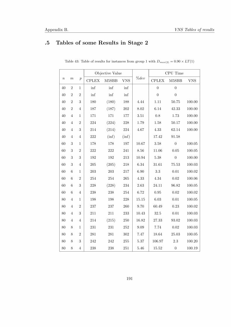
Appendix B. VNS Tables of results
.5 Tables of some Results in Stage 2
Table 43: Table of results for instances from group 1 with Dmax(2) = 0.90× LT (1)
Objective Value CPU Timen m p
CPLEX M5SBB VNS%dev
CPLEX M5SBB VNS
40 2 1 inf inf inf 0 0
40 2 2 inf inf inf 0 0
40 2 3 180 (180) 188 4.44 1.11 50.75 100.00
40 2 4 187 (187) 202 8.02 6.14 42.33 100.00
40 4 1 171 171 177 3.51 0.8 1.73 100.00
40 4 2 224 (224) 228 1.79 1.58 50.17 100.00
40 4 3 214 (214) 224 4.67 4.33 62.14 100.00
40 4 4 222 (inf) (inf) 17.42 91.58
60 3 1 178 178 197 10.67 3.58 0 100.05
60 3 2 222 222 241 8.56 11.06 0.05 100.05
60 3 3 192 192 213 10.94 5.38 0 100.00
60 3 4 205 (205) 218 6.34 31.61 75.53 100.03
60 6 1 203 203 217 6.90 3.3 0.01 100.02
60 6 2 254 254 265 4.33 4.34 0.02 100.06
60 6 3 228 (228) 234 2.63 24.11 96.82 100.05
60 6 4 238 238 254 6.72 0.95 0.02 100.02
80 4 1 198 198 228 15.15 6.03 0.01 100.05
80 4 2 237 237 260 9.70 60.49 0.23 100.02
80 4 3 211 211 233 10.43 32.5 0.01 100.03
80 4 4 214 (215) 250 16.82 27.33 93.02 100.03
80 8 1 231 231 252 9.09 7.74 0.02 100.03
80 8 2 281 281 302 7.47 18.64 25.03 100.05
80 8 3 242 242 255 5.37 106.97 2.3 100.20
80 8 4 238 238 251 5.46 15.52 0 100.19
191
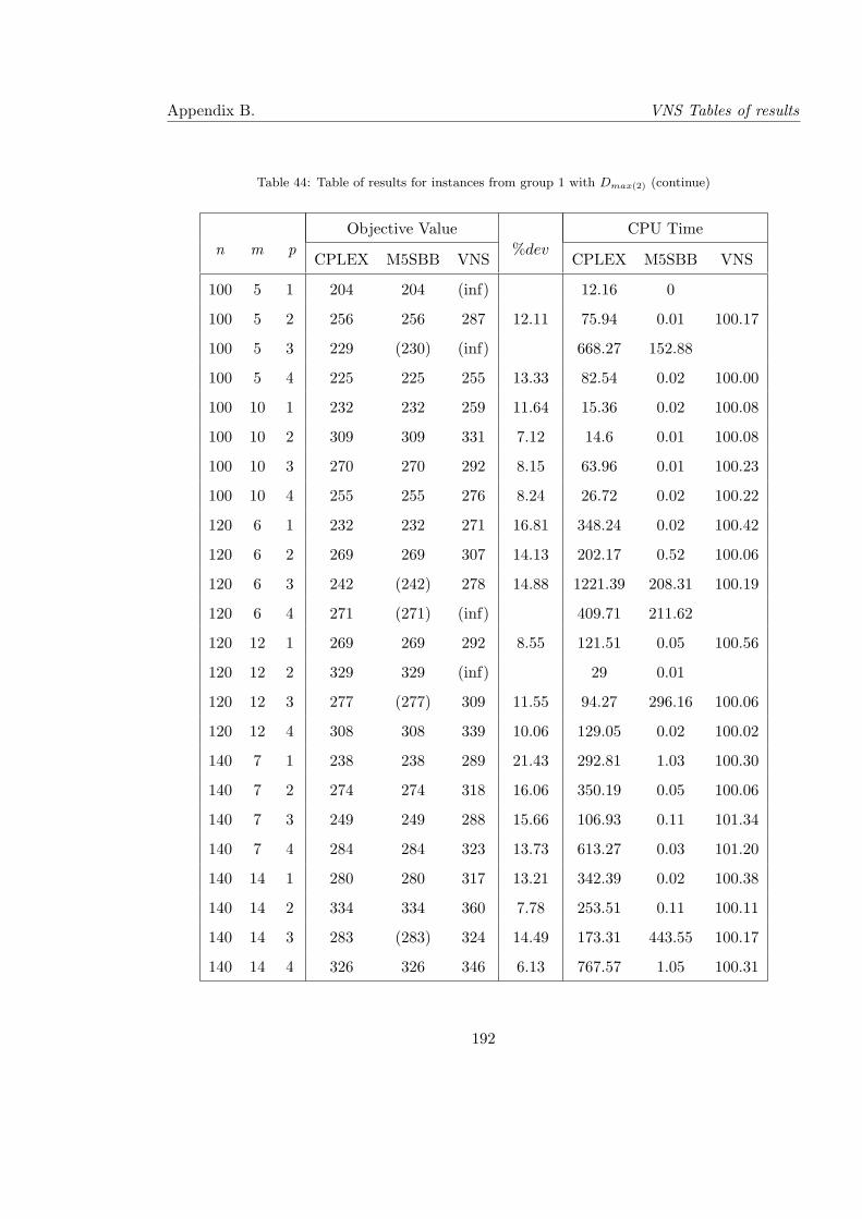
Appendix B. VNS Tables of results
Table 44: Table of results for instances from group 1 with Dmax(2) (continue)
Objective Value CPU Timen m p
CPLEX M5SBB VNS%dev
CPLEX M5SBB VNS
100 5 1 204 204 (inf) 12.16 0
100 5 2 256 256 287 12.11 75.94 0.01 100.17
100 5 3 229 (230) (inf) 668.27 152.88
100 5 4 225 225 255 13.33 82.54 0.02 100.00
100 10 1 232 232 259 11.64 15.36 0.02 100.08
100 10 2 309 309 331 7.12 14.6 0.01 100.08
100 10 3 270 270 292 8.15 63.96 0.01 100.23
100 10 4 255 255 276 8.24 26.72 0.02 100.22
120 6 1 232 232 271 16.81 348.24 0.02 100.42
120 6 2 269 269 307 14.13 202.17 0.52 100.06
120 6 3 242 (242) 278 14.88 1221.39 208.31 100.19
120 6 4 271 (271) (inf) 409.71 211.62
120 12 1 269 269 292 8.55 121.51 0.05 100.56
120 12 2 329 329 (inf) 29 0.01
120 12 3 277 (277) 309 11.55 94.27 296.16 100.06
120 12 4 308 308 339 10.06 129.05 0.02 100.02
140 7 1 238 238 289 21.43 292.81 1.03 100.30
140 7 2 274 274 318 16.06 350.19 0.05 100.06
140 7 3 249 249 288 15.66 106.93 0.11 101.34
140 7 4 284 284 323 13.73 613.27 0.03 101.20
140 14 1 280 280 317 13.21 342.39 0.02 100.38
140 14 2 334 334 360 7.78 253.51 0.11 100.11
140 14 3 283 (283) 324 14.49 173.31 443.55 100.17
140 14 4 326 326 346 6.13 767.57 1.05 100.31
192
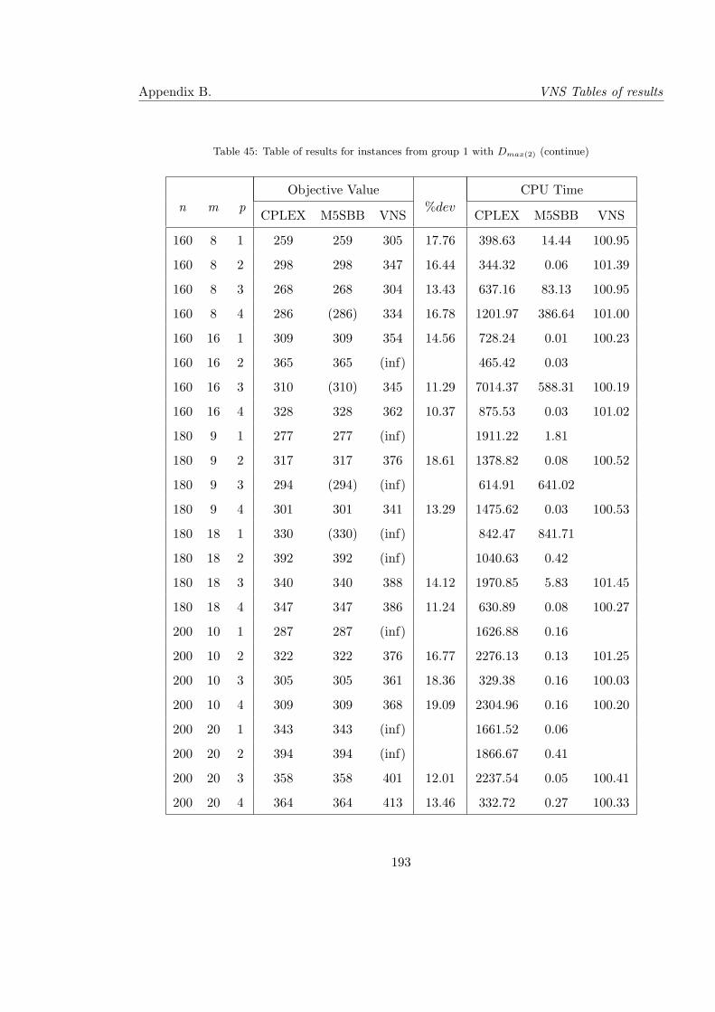
Appendix B. VNS Tables of results
Table 45: Table of results for instances from group 1 with Dmax(2) (continue)
Objective Value CPU Timen m p
CPLEX M5SBB VNS%dev
CPLEX M5SBB VNS
160 8 1 259 259 305 17.76 398.63 14.44 100.95
160 8 2 298 298 347 16.44 344.32 0.06 101.39
160 8 3 268 268 304 13.43 637.16 83.13 100.95
160 8 4 286 (286) 334 16.78 1201.97 386.64 101.00
160 16 1 309 309 354 14.56 728.24 0.01 100.23
160 16 2 365 365 (inf) 465.42 0.03
160 16 3 310 (310) 345 11.29 7014.37 588.31 100.19
160 16 4 328 328 362 10.37 875.53 0.03 101.02
180 9 1 277 277 (inf) 1911.22 1.81
180 9 2 317 317 376 18.61 1378.82 0.08 100.52
180 9 3 294 (294) (inf) 614.91 641.02
180 9 4 301 301 341 13.29 1475.62 0.03 100.53
180 18 1 330 (330) (inf) 842.47 841.71
180 18 2 392 392 (inf) 1040.63 0.42
180 18 3 340 340 388 14.12 1970.85 5.83 101.45
180 18 4 347 347 386 11.24 630.89 0.08 100.27
200 10 1 287 287 (inf) 1626.88 0.16
200 10 2 322 322 376 16.77 2276.13 0.13 101.25
200 10 3 305 305 361 18.36 329.38 0.16 100.03
200 10 4 309 309 368 19.09 2304.96 0.16 100.20
200 20 1 343 343 (inf) 1661.52 0.06
200 20 2 394 394 (inf) 1866.67 0.41
200 20 3 358 358 401 12.01 2237.54 0.05 100.41
200 20 4 364 364 413 13.46 332.72 0.27 100.33
193