dissimilarity measures for hidden markov models and their
TRANSCRIPT
Tampere University of Technology
Department of Information Technology
Matti Vihola
Dissimilarity Measures for Hidden Markov
Models and Their Application in Multilingual
Speech Recognition
Master of Science Thesis
Subject approved by the Department Councilon November 14th 2001Examiners: Prof. Jukka Saarinen
Prof. Jaakko AstolaDr. Tech. Petri SalmelaLic. Tech. Janne Suontausta

Preface
This thesis is a part of the User-Oriented Information Technology (USIX) technology pro-gram directed by the Finnish National Technology Agency (Tekes). The work has beencarried out at the Institute of Signal Processing, Department of Information Technology,Tampere University of Technology; in collaboration with Nokia Research Center and De-partment of Phonetics, University of Turku.
I wish to thank Dr. Tech. Petri Salmela for advice and persistent guidance throughout thewriting process. I am also grateful for Professor Jukka Saarinen, Professor Jaakko Astolaand Lic. Tech. Janne Suontausta for advice and contructive criticism.
I express my gratitude to all the members of the multilingual speech recognition projectboth at the Institute of Signal Processing and at the Institute of Digital and ComputerSystems. Furthermore, thanks goes to all the colleague researchers in the Audio ResearchGroup. It has been a pleasure working with you all!
Tampere, 6th May 2002
Matti Vihola
Opiskelijankatu 4 E 28933720 TampereTel. (+358)400-908508
ii

Contents
Preface ii
Contents iii
Tiivistelma v
Abstract vi
1 Introduction 1
2 Automatic Speech Recognition 42.1 Classification of Speech Recognition Tasks . . . . . . . . . . . . . . . . . . . 42.2 Typical Structure of a Modern Speech Recognition System . . . . . . . . . . 62.3 Feature Extraction Unit . . . . . . . . . . . . . . . . . . . . . . . . . . . . . 62.4 Hidden Markov Models . . . . . . . . . . . . . . . . . . . . . . . . . . . . . 8
2.4.1 HMM Representation . . . . . . . . . . . . . . . . . . . . . . . . . . 92.4.2 Speech Recognition Using HMMs . . . . . . . . . . . . . . . . . . . . 102.4.3 Training of HMMs . . . . . . . . . . . . . . . . . . . . . . . . . . . . 12
2.5 Speaker Adaptation . . . . . . . . . . . . . . . . . . . . . . . . . . . . . . . 142.5.1 Maximum Likelihood Linear Regression . . . . . . . . . . . . . . . . 15
3 Multilingual Speech Recognition 163.1 Multilingual Speech Corpora . . . . . . . . . . . . . . . . . . . . . . . . . . 163.2 Portability of Speech Technology . . . . . . . . . . . . . . . . . . . . . . . . 17
3.2.1 Language-dependency of Speech Recognition Systems . . . . . . . . 173.2.2 Cross-language Transfer . . . . . . . . . . . . . . . . . . . . . . . . . 183.2.3 Language Adaptation . . . . . . . . . . . . . . . . . . . . . . . . . . 18
3.3 Multilingual Acoustic Modeling . . . . . . . . . . . . . . . . . . . . . . . . . 193.3.1 Knowledge-Based Methods . . . . . . . . . . . . . . . . . . . . . . . 203.3.2 Computational Methods . . . . . . . . . . . . . . . . . . . . . . . . . 213.3.3 Language Identification . . . . . . . . . . . . . . . . . . . . . . . . . 21
4 Dissimilarity Measures for HMMs 234.1 Measures Based on Confusion Matrix . . . . . . . . . . . . . . . . . . . . . . 24
4.1.1 Estimation of a Confusion Matrix for Phoneme Model HMMs . . . . 254.1.2 Conversion of a Confusion Matrix into a Dissimilarity Matrix . . . . 27
4.2 Measures Based on Kullback-Leibler Divergence . . . . . . . . . . . . . . . . 294.2.1 Monte-Carlo Techniques . . . . . . . . . . . . . . . . . . . . . . . . . 304.2.2 Monte-Carlo Estimates based on Speech Data . . . . . . . . . . . . . 304.2.3 Closed Form Solutions based on Simplifying Approximations . . . . 31
iii

CONTENTS
5 Experimental Setup and Results 345.1 Speech Corpora and Front-End . . . . . . . . . . . . . . . . . . . . . . . . . 345.2 Baseline Speech Recognition Systems and Data Sets . . . . . . . . . . . . . 355.3 Multilingual Recognition Systems . . . . . . . . . . . . . . . . . . . . . . . . 36
5.3.1 Knowledge-based Multilingual Recognition Systems . . . . . . . . . 375.3.2 Multilingual Recognition Systems based on Dissimilarity Measures . 385.3.3 Unseen Languages . . . . . . . . . . . . . . . . . . . . . . . . . . . . 40
5.4 Comparison of Recognition Results . . . . . . . . . . . . . . . . . . . . . . . 42
6 Conclusions 46
A Transformation Classes for MLLR 52A.1 Mixture Component Level Definition . . . . . . . . . . . . . . . . . . . . . . 52A.2 HMM Level Definition . . . . . . . . . . . . . . . . . . . . . . . . . . . . . . 53
iv
Tiivistelma
TAMPEREEN TEKNILLINEN KORKEAKOULUTietotekniikan osastoSignaalinkasittelyn laitosVIHOLA, MATTI: Erilaisuusmitat piilo-Markov -malleille ja niiden kaytto monikielisessa
puheentunnistuksessa.Diplomityo, 51 s.; liite, 3 s.Tarkastajat: Prof. Jukka Saarinen, Prof. Jaakko Astola, TkT Petri Salmela, TkL Janne
Suontausta (Nokia Research Center).Rahoittajat: Teknologian kehittamiskeskus (Tekes), Nokia Research Center.Toukokuu 2002Avainsanat: Erilaisuusmitta, etaisyysmitta, Kullback-Leibler -divergenssi, monikielisyys,
piilo-Markov -malli, puheentunnistus, ryhmittely, sekaannusmatriisi.
Automaattista puheentunnistusta voidaan jo kayttaa joihinkin kuluttajasovelluksiin. In-tensiivista tutkimusta tarvitaan kuitenkin viela esimerkiksi monikielituen kehittamisessa.Tama tyo kasittelee monikielista akustista mallinnusta, erityisesti monikielisten akustistenmallien maaraamista. Eras menetelma monikielisen puheentunnistusjarjestelman toteut-tamiseksi pohjautuu valmiiksi koulutettuun joukkoon kieliriippuvia tunnistusjarjestelmia.Naiden jarjestelmien akustisten mallien valinen erilaisuus mitataan kayttaen tiettya erilai-suusmittaa, ja sita hyvaksikayttaen ryhmitellaan akustiset mallit. Tarkoituksena on saadaaikaiseksi pieni, mutta kattava joukko akustisia malleja, jotka jaetaan eri kielten kesken.
Tassa tyossa kaydaan lapi erilaisuusmittoja piilo-Markov -malleille (HMM). Mittoihin,joita voidaan kayttaa akustisten mallien ryhmittelyyn, kiinnitetaan erityista huomiota.Kaikki tyossa esitetyt mitat pohjautuvat joko sekaannusmatriisiestimaattiin tai Kullback-Leibler (KL) -divergenssin estimaattiin tai sen approksimaatioon. Tyossa luodaan katsausedella mainittuihin mittoihin, ja esitetaan muunnettuja menetelmia estimaattien tarkenta-miseksi. Tyossa esitellaan lisaksi kaksi approksimaatiota KL -divergenssista, jotka voidaanesittaa suljetussa muodossa. Naiden approksimaatioiden laskennalliset kustannukset ovaterittain alhaiset, mutta niita voidaan soveltaa ainoastaan HMM:iin, joilla on multinormaa-lit havaintojakaumat, seka tietynlainen mallirakenne.
Koejarjestelyssa erilaisuusmittoja tarkasteltiin monikielisten akustisten mallien maaritta-misessa. Kokeissa monikieliset tunnistimet rakennettiin viidelle kielelle, jotka olivat englan-ti, espanja, italia, saksa ja suomi. Monikielinen puheentunnistusjarjestelma, jossa on 64akustista mallia, opetettiin jokaisen erilaisuusmitan tuottaman akustisten mallien ryhmit-telyn perusteella. Naita tunnistusjarjestelmia verrattiin seka keskenaan, etta monikielisiinjarjestelmiin, joissa akustisten mallien ryhmittely ja maarittely oli suoritettu foneettisentiedon pohjalta. Monikielisten tunnistusjarjestelmien tunnistustarkkuus arvioitiin puhuja-riippumattomassa irrallisten sanojen tunnistuksessa. Kieliriippuvilla jarjestelmilla keski-maarainen tunnistusprosentti sanoille oli noin 89%. Monikielisten jarjestelmien tunnistus-prosentti vaihteli valilla 82–84%. Erot monikielisten jarjestelmien valilla olivat siten pienia.Monikielisia jarjestelmia kokeiltiin myos kahden uuden kielen, ranskan ja ruotsin, tunnis-tamisessa. Naiden kielten kieliriippuville jarjestelmille keskimaarainen tunnistusprosenttioli noin 84%. Vastaava prosentti monikielisille jarjestelmille vaihteli valilla 60–64%.
Abstract
TAMPERE UNIVERSITY OF TECHNOLOGYDepartment of Information TechnologyInsitute of Signal ProcessingVIHOLA, MATTI: Dissimilarity Measures for Hidden Markov Models and Their Appli-
cation in Multilingual Speech Recognition.Master of Science thesis, 51 pages; Appendix, 3 pages.Examiners: Prof. Jukka Saarinen, Prof. Jaakko Astola, Dr. Tech. Petri Salmela,
Lic. Tech. Janne Suontausta (Nokia Research Center).Funding: Finnish National Technology Agency (Tekes), Nokia Research Center.May 2002Keywords: Clustering, confusion matrix, dissimilarity measure, distance measure, hidden
Markov model, Kullback-Leibler divergence, multilinguality, speech recognition.
Although automatic speech recognition (ASR) technology is mature enough for some con-sumer products, intensive research is still needed to obtain e.g. the support for multiplelanguages. This thesis contributes to multilingual (ML) acoustic modeling, especially tothe techniques that can be used for defining a set of ML acoustic models for ML ASRsystem. One starting point for the development of such a system is first to train a set oflanguage dependent (LD) ASR systems. Based on some measure of dissimilarity betweenthe obtained LD acoustic models, the objective is to reduce the acoustic model set into acompact set of models that are shared across the languages.
In this thesis, the dissimilarity measures for hidden Markov models (HMMs), especiallythose that are applicable for the clustering of acoustic HMMs, are covered. All the measuresare based either on a confusion matrix estimate, or on an estimate or an approximationof the Kullback-Leibler (KL) divergence. This thesis reviews a number of such methods,and also proposes some modifications to get more accurate KL divergence and confusionmatrix estimates. In addition, two closed-form approximations of the KL divergence areproposed. These closed-form approximations have very low computational cost, but theyare restricted for HMMs with Gaussian emission densities and employ assumptions of theHMM topology.
The dissimilarity measures were experimented in the definition of the set of ML phonemodels. One ML ASR system having 64 phone models was trained for each phone clus-ter definition obtained from the corresponding dissimilarity measure. The systems weretrained for five languages: English, Finnish, German, Italian and Spanish. The obtainedASR systems were compared both against each other, and to the alternative ML ASR sys-tems having phone clusters determined solely by expert knowledge. The performances ofthese multilingual recognizers were evaluated in the task of speaker independent isolatedword recognition. The average word recognition rate (WRR) of the baseline LD recogni-tion systems was approximately 89%, while the average WRRs of the ML systems variedbetween 82–84%. Small differences were observed in the recognition accuracies of the dif-ferent ML recognition systems. The ML systems were tested also with two new languages,French and Swedish. In the experiments, the average WRR was 84% for the baseline LDsystems, while the average WRR of the ML ASR system dropped to 60–64%.

List of Acronyms
ASR Automatic speech recognitionBW Baum-WelchDCT Discrete cosine transformDFT Discrete Fourier transformEM Expectation-maximizationGMM Gaussian mixture modelHMM Hidden Markov modelHTK Hidden Markov Model ToolkitIPA International Phonetic AssociationKL Kullback-LeiblerLD Language dependentLID Language identificationMAP Maximum a posterioriMC Monte-CarloMFCC Mel-frequency cepstral coefficientML MultilingualMLE Maximum likelihood estimateMLLR Maximum likelihood linear regressionPDF Probability density functionSAMPA Speech Assessment Methods Phonetic AlphabetSD Speaker dependentSI Speaker independentSIL Silence modelSP Short pause modelWRR Word recognition rate
vii

List of Symbols
General notations
A,B,C . . . Matricesa, b, c . . . Vectorsa, b, c . . . ScalarsA,B, C . . . Setsaij Element of matrix AA−1 Inverse of matrix A|A| Determinant of matrix AbT Transpose of vector bcardA Cardinality, i.e. number of elements in the set Adim b Dimension of vector bE
{f(Oλ)
}Expectation of function f of a random variable Oλ with distributionλ
fD(·; θ) The PDF of distribution D with parameters θt(x,y) Tanimoto similarity ratio of vectors x and ytrA Trace of matrix Ax[n] n:th sample of a discrete-time signal xµ Mean vector of a random distributionΣ Covariance matrix of a random distribution{x : cond(x)} A set of all such elements x that fulfill the condition cond(·)[c, d]T A vector consisting of elements c and d(a, b) Ordered set containing the elements a and b
Mel-frequency cepstral coefficients
Ci The ith cepstral coefficient of a frameD Dimension of an observation feature vector oE The energy estimate of a frameO Observation vector sequenceot Observation vector occurring at time instant t∆C First time derivative coefficient corresponding C∆2C Second time derivative coefficient corresponding C
Hidden Markov models
A The transition matrix of a HMMbj(o) The likelihood of emission distribution of state j of a HMM
viii

LIST OF SYMBOLS
P (O) Likelihood of observation sequence OP (λ) A priori probability of model λP (O | λ) Conditional likelihood of O given λP ∗(O | λ) The likelihood of the most likely state sequence of O given λq State sequence vectorqt State at time instant tq∗ The most likely state sequenceQ(T ) Set of state sequences of length T
Q(λ, λ) Baum’s auxiliary functionwjk The weight of the kth mixture component of a GMM of the state j
of a HMMαt(j) Forward variable of state j at time instant tβt(i) Backward variable of state i at time instant tγt(j, k) The a posteriori probability of an observation at time instant t origi-
nating from the kth mixture component of the state j of a HMMδt(i) The accumulated likelihood of the most likely state sequence up to
state i at time instant tδ∗m(κ) The accumulated likelihood of the most likely state sequence of model
κΘ Parameter set of all emission densities of a HMMθjk Parameters of a mixture density component k of the state j of a HMMκ The parameter set of a HMMλ The parameter set of a HMMλ⊕ κ The concatenated HMM consisting of λ and κξt(i, j) The probability of being in state i at time t and state j at time t+ 1π Initial state distribution of a HMMψt(i) The previous state of the partial most likely state sequence up to state
i at time instant t
Dissimilarity measures
C Confusion matrixCX The estimate of the confusion matrix according to the estimation
method XD Dissimilarity matrixI(λ : κ) The directed KL divergence from distribution λ to κIX(λ : κ) The estimate of the directed KL divergence from λ to κ according to
the estimation method XJ(λ, κ) The KL divergence between distributions λ and κLLR(O | λ, κ) Logarithmic likelihood ratio function of O given the models λ and κS Similarity matrixSC(O | λ) Likelihood score function of O given the model λ
ix

Chapter 1
Introduction
An infant mimics speech sounds at a very young age, and learns to speak without ex-plicit teaching quickly. A recent reasearch has proved an interesing result: even a new-born child (1-7 days old) can distinguish between different vowel sounds, while being fastasleep [Cheour et al. 2002]. If speech is such a built-in communication method for humans,why cannot machines be operated by voice commands?
Automatic speech recognition (ASR), i.e. recognition of human speech with a machine, hasbeen researched since the 1950s [Gold and Morgan 2000]. Such a natural thing for humansas speech recognition has showed to be a very challenging task for machines. Despite thedifficulties, the persistent research in the area ever since the 1950s has yielded marks ofprogress. Today, ASR technology has been applied to consumer products, e.g. name dialersin mobile handsets, telephone number queries and train timetable retreival systems. Somevery fundamental issues have risen in employing ASR for the purposes of such applications.These include e.g. robustness, espcially for noise and changing acoustic conditions, andsupport for multiple languages. The speech interface is natural and convenient to use onlywhen it is robust, and can be operated with the native language of the user. Therefore,a comprehensive support for languages is one of the key characteristics that the speech-driven applications need to fulfill before a true widespread acceptance can be achieved.
The spoken languages apparently share common acoustic features. This is evident as thesource of the speech signal is always the human speech production system, regardless ofthe language. Different sounds that are produced by this system while speaking are knownas phonemes. Phonemes are the atomic units of speech, or language, meaning that bychanging a phoneme in a word, the meaning of the word can change. For example, bychanging the first phoneme in the word “pet”, we get the word “set”1. The phonemes canbe classified by their articulatory characteristics, e.g. to resonants and obstruents (whetherthe vocal tract is blocked or not), consonants and vowels, and so on2. Speech recognitionsystems are often built using the phonemes as modeling units. One phoneme, or allophone3,is represented with one acoustic model, most often a hidden Markov model (HMM).
This thesis concerns finding the phonemes, or allophones, that are similar to each otherover a set of languages. This information has been employed previously in the definition
1. Interestingly, in English, the change of the written form of a word doesn’t necessarily affect the pro-nunciation, i.e. the phonemic representation. For example, the phonemic content of the word “sea”, /si�/,is identical to the word “see”. Conversely, the phonemic content of the written word “read” depends on thetense, either /ri�d/ or /red/.2. Such categorization of phonemes is shown in Figure A.2 in Appendix A.3. Allophone is a phoneme in a certain context. For example, the two allophones of the phoneme /l/ inthe words “feeling” and “alarm” sound rather different.
1

CHAPTER 1. INTRODUCTION
Time [s]
Fre
quen
cy [H
z]
0 0.1 0.2 0.3 0.4 0.5 0.6 0.70
500
1000
1500
2000
2500
3000
3500
4000
p �� za
Time [s]
Fre
quen
cy [H
z]
0 0.1 0.2 0.3 0.4 0.50
500
1000
1500
2000
2500
3000
3500
4000
p o i s t �
b
Figure 1.1: (a) Spectrogram of the English word “pause” /p��z/ and (b) the Finnish word“poista” /poist�/.
of a set of multilingual (ML) phone HMMs [Kohler 2000]. This means in practice that thephonemes of a set of languages are grouped, or clustered, such that the number of clustersis smaller than the original number of language dependent phonemes. The Figure 1.1shows spectrograms of two uttered words, English “pause” and Finnish “poista” (“remove”in English). In this example, the English /p/ and Finnish /p/ could be represented with acommon ML phone4 model /p/. In addition, two pairs of similar phonemes can be found:English /��/ and Finnish /o/; and English /z/ and Finnish /s/. The number of the MLphone models could be reduced from nine to six in this example, if the above tying of thephonemes were applied.
The search for these similar phonemes has been previously performed by comparing theacoustic models, HMMs, that are used in the speech recognition system [Andersen et al.1994, Kohler 2001]. The proximity of the HMMs has been measured by employing some
4. In this thesis, “phone” refers to a ML acoustic model that represents a set of LD phoneme models.
2

CHAPTER 1. INTRODUCTION
dissimilarity measure, which measures how discriminating two HMMs are. This thesisreviews the measures introduced for this task. In addition, four modified measures areproposed to give an increased accuracy for the previously proposed measures, and twomeasures having low computational cost are introduced. The behavior of the measures iscompared, when they are applied in the task of phoneme model clustering.
This thesis consists of the following chapters. In Chapter 2, the methods used in modernspeech recognition are discussed. This discussion covers the methods often used for the pre-processing of the speech signal and statistical pattern recognition, which are Mel-frequencycepstral coefficients (MFCCs) and HMMs, respectively. In Chapter 3, an overview of theissues covered by the research in the field of multilingual speech recognition is given. Themain topic of the thesis, the dissimilarity measures for HMMs, is discussed in Chapter 4.The previously proposed methods are reviewed, and some novel techniques are proposed.Chapter 5 covers the experiments before the concluding remarks given in Chapter 6.
3

Chapter 2
Automatic Speech Recognition
Machine recognition of human speech, often referred to as automatic speech recognition(ASR), has been investigated from the early 1950s [Gold and Morgan 2000]. The researchin the area has been rather intense since the late 1970s. During 1980s, statistical model-ing, namely the hidden Markov models (HMMs), started to replace the earlier template-matching-based methods in ASR [Rabiner 1993]. Today, the most successful ASR systemsare based on these statistical models, of course flavored with lots of adjustments andimprovements.
In this chapter, a brief overview of the modern ASR systems is given. First of all, thecategorization of the speech recognition tasks is discussed in Section 2.1. After that, Sec-tion 2.2 outlines the structure of a typical ASR system. This system can be roughly dividedinto two main units which are the feature extraction unit, and the pattern classifier unit.These two units are often also referred as the front-end and the back-end, respectively.The derivation of the typical Mel-frequency cepstral coefficient (MFCC) features producedby the front-end unit is covered in Section 2.3. After that, the techniques involved in thepattern classifier unit are reviewed briefly in Section 2.4. These include the concept ofHMMs and some essential training and decoding algorithms. Finally, the speaker adap-tation techniques, especially maximum likelihood linear regression (MLLR), are discussedin Section 2.5.
2.1 Classification of Speech Recognition Tasks
Speech recognition systems are nowadays implemented in a very application dependentmanner. This is mainly due to limited resources and the many obstacles still faced in thefield of speech recognition. The obvious consequence of application oriented implementa-tions is that they may not work well in some other application domain. In the following,some characteristics are explained that discriminate the different ASR tasks [Adda-Decker2001, Kiss 2001, Laurila 2000, Viikki 1999, Waibel et al. 2000].
Vocabulary size: Today, the systems with small vocabulary can distinguish some tensof words. The medium vocabulary size ranges from hundred to thousand words andthe large vocabulary systems range up to 100000 words [Viikki 1999]. The numberof words in the vocabulary affects both the recognition accuracy and the speed ofthe recognition process. In addition, the choice of the acoustic units depends onthe size of the vocabulary. The whole word models can be used as acoustic units ina small vocabulary ASR task, while these units are replaced with subword modelsas the vocabulary becomes larger. The typical subword units represent phonemes,
4

CHAPTER 2. AUTOMATIC SPEECH RECOGNITION
allophones or syllables. Furthermore, the type of the vocabulary can be fixed, suchas in a digit recognition, or dynamic, such as in a name dialer in a mobile handset.
Continuous, connected or isolated word recognition: In an isolated word recogni-tion task, the recognition system forms a hypothesis of the uttered word or phraseas a single entity. Connected word recognition can be considered a step forward,since the user is allowed to speak several words at a time, but a short pause hasto be left between the words. However, the word boundaries are hard to find innatural speech due to coarticulation, which makes the task of continuous speechrecognition challenging. Coarticulation of words means that they are articulatedconsecutively after each other with no inter-word pause. A language model is notnecessarily needed in isolated word recognition, but in continous ASR, languagemodeling is an important issue.
Speaker dependent or independent systems: The speaker independency of an ASRsystem is a desired feature in general. A speaker independent (SI) system can copewith different speakers, speaking styles and even dialects. However, the speakerdependent (SD) ASR systems outperform the SI systems in recognition accuracybecause the acoustic models of the SD system have to cope with smaller variabilityof acoustic features in speech [Viikki 1999]. The direct training of SD recognitionsystem is unfeasible in most cases, as hours of speech material may be neededfrom the target speaker1. Speaker dependent speech recognition system can beobtained by adapting SI recognition system either continuously, i.e. performing theadaptation online, or with relatively small adaptation data set. Such adaptationtechniques are discussed more in detail in Section 2.5.1.
Language dependent or multilingual systems: Typically the ASR systems are lim-ited to only a single language. The support for multiple languages in ASR systemshas emerged as the first widely spread applications have been introduced [Waibelet al. 2000]. The multilinguality of an ASR system can be viewed somehow analo-gous to speaker independency. The multilingual speech recognition is discussed inChapter 3 in more detail.
Environmental robustness: Many speech recognition applications work well in labo-ratory, but they have difficulties in realistic environments. Their applicability cancollapse very quickly instead of graceful deterioration when the signal is corruptede.g. with background noise or microphone distortion. In general, the ASR systemswork well in conditions similar to the conditions of the acoustic material used dur-ing training. The real world ASR applications demand the recognition system tobe robust for various acoustic and noise conditions. The techniques that are usedin noise robust speech recognition can be grouped into the following categories:noise robust feature vectors, techniques compensating noise from feature vectorsand model parameter adaptation and compensation techniques [Furui 1995, Junqua2000].
The field of the speech recognition research can be stated extensive. Isolated word rec-ognition task with a small vocabulary is a rather straightforward pattern classificationtask. However, considering the recognition of continuous conversational speech with largevocabulary, the semantics and pragmatics involved in the discussion must be included toachieve accurate recognition performance. The scope of this thesis covers pattern classi-fication and acoustic modeling of speech. Language modeling and understanding are notdiscussed.
1. Practically, the SD system is feasible to build for a small vocabulary ASR task.
5
CHAPTER 2. AUTOMATIC SPEECH RECOGNITION
Speechwaveform
Front-end
Acoustic models
Pattern matching
Language model& lexicon
Back-end
Recognitionhypothesis
"forty-two"
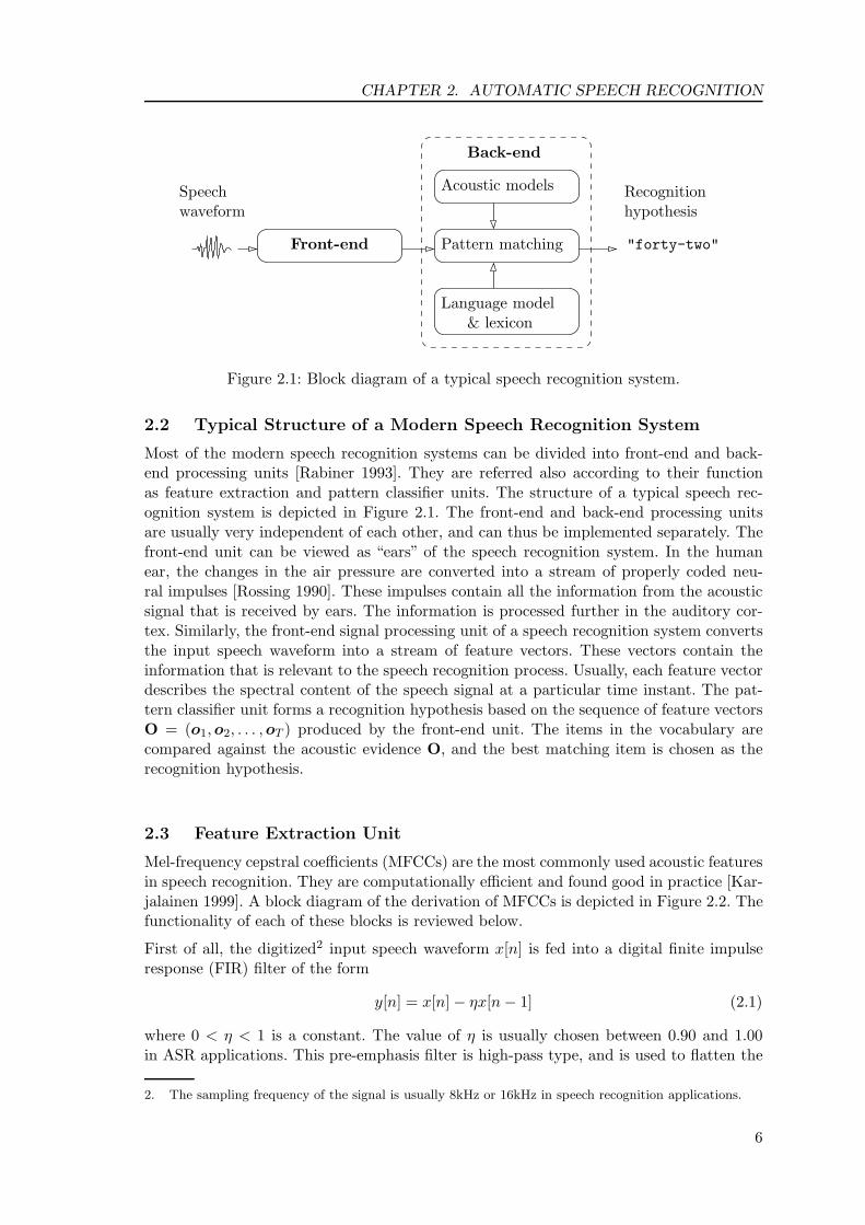
Figure 2.1: Block diagram of a typical speech recognition system.
2.2 Typical Structure of a Modern Speech Recognition System
Most of the modern speech recognition systems can be divided into front-end and back-end processing units [Rabiner 1993]. They are referred also according to their functionas feature extraction and pattern classifier units. The structure of a typical speech rec-ognition system is depicted in Figure 2.1. The front-end and back-end processing unitsare usually very independent of each other, and can thus be implemented separately. Thefront-end unit can be viewed as “ears” of the speech recognition system. In the humanear, the changes in the air pressure are converted into a stream of properly coded neu-ral impulses [Rossing 1990]. These impulses contain all the information from the acousticsignal that is received by ears. The information is processed further in the auditory cor-tex. Similarly, the front-end signal processing unit of a speech recognition system convertsthe input speech waveform into a stream of feature vectors. These vectors contain theinformation that is relevant to the speech recognition process. Usually, each feature vectordescribes the spectral content of the speech signal at a particular time instant. The pat-tern classifier unit forms a recognition hypothesis based on the sequence of feature vectorsO = (o1,o2, . . . ,oT ) produced by the front-end unit. The items in the vocabulary arecompared against the acoustic evidence O, and the best matching item is chosen as therecognition hypothesis.
2.3 Feature Extraction Unit
Mel-frequency cepstral coefficients (MFCCs) are the most commonly used acoustic featuresin speech recognition. They are computationally efficient and found good in practice [Kar-jalainen 1999]. A block diagram of the derivation of MFCCs is depicted in Figure 2.2. Thefunctionality of each of these blocks is reviewed below.
First of all, the digitized2 input speech waveform x[n] is fed into a digital finite impulseresponse (FIR) filter of the form
y[n] = x[n] − ηx[n− 1] (2.1)
where 0 < η < 1 is a constant. The value of η is usually chosen between 0.90 and 1.00in ASR applications. This pre-emphasis filter is high-pass type, and is used to flatten the
2. The sampling frequency of the signal is usually 8kHz or 16kHz in speech recognition applications.
6
CHAPTER 2. AUTOMATIC SPEECH RECOGNITION
...
Speechwaveform
Featurevectors
Pre-emphasis Windowing DFT
Mel-scalingLogarithmDCT
dB
f
ff
M
M
M
M
log MC
i
t
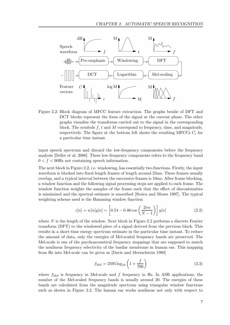
Figure 2.2: Block diagram of MFCC feature extraction. The graphs beside of DFT andDCT blocks represent the form of the signal at the current phase. The othergraphs visualize the transforms carried out to the signal in the correspondingblock. The symbols f , t and M correspond to frequency, time, and magnitude,respectively. The figure at the bottom left shows the resulting MFCCs Ci fora particular time instant.
input speech spectrum and discard the low-frequency components before the frequencyanalysis [Deller et al. 2000]. These low-frequency components refers to the frequency band0 < f < 90Hz not containing speech information.
The next block in Figure 2.2, i.e. windowing, has essentially two functions. Firstly, the inputwaveform is blocked into fixed length frames of length around 25ms. These frames usuallyoverlap, and a typical interval between the successive frames is 10ms. After frame blocking,a window function and the following signal processing steps are applied to each frame. Thewindow function weights the samples of the frame such that the effect of discontinuitiesis minimized and the spectral estimate is smoothed [Stoica and Moses 1997]. The typicalweighting scheme used is the Hamming window function
z[n] = w[n]y[n] =[0.54 − 0.46 cos
(2πnN − 1
)]y[n] (2.2)
where N is the length of the window. Next block in Figure 2.2 performs a discrete Fouriertransform (DFT) to the windowed piece of a signal derived from the previous block. Thisresults in a short-time energy spectrum estimate in the particular time instant. To reducethe amount of data, only the energies of Mel-scaled frequency bands are preserved. TheMel-scale is one of the psychoacoustical frequency mappings that are supposed to matchthe nonlinear frequency selectivity of the basilar membrane in human ear. This mappingfrom Hz into Mel-scale can be given as [Davis and Mermelstein 1980]
fMel = 2595 log10
(1 +
f
700
)(2.3)
where fMel is frequency in Mel-scale and f frequency in Hz. In ASR applications, thenumber of the Mel-scaled frequency bands is usually around 20. The energies of thesebands are calculated from the magnitude spectrum using triangular window functionssuch as shown in Figure 2.2. The human ear works nonlinear not only with respect to
7
CHAPTER 2. AUTOMATIC SPEECH RECOGNITION
frequencies, but also with the signal power. The perceived power of the audio signal,i.e. loudness, is roughly logarithmic compared to the power of the signal [Rossing 1990].This is why a logarithm of each of the bandwise energies is taken.
In order to obtain MFCCs, the last block in Figure 2.2 performs the discrete cosine trans-form (DCT) to the logarithmic energy estimates of the Mel-scaled frequency bands [Delleret al. 2000]. Typically only the first 13 DCT coefficients are preserved to form the basis ofa feature vector. The DCT reduces correlation between the elements of the feature vector,which is useful in the back-end processing3. Usually the zeroth MFCC, C0, is replacedwith an energy estimate E of the frame. This energy estimate is considered less noisy thanC0. An inter-frame context-dependency is also often supplemented to the feature vector bycalculating the first and second time derivative coefficients of the consecutive MFCC-basedfeature vectors [Furui 1986]. Finally, the resulting feature vector has the form
o =[E,C1, · · ·CL,∆E,∆C1, · · ·∆CL,∆2E,∆2C1, · · ·∆2CL
]T (2.4)
where E is the energy and Ci the ith cepstral coefficient of the frame. In addition, thenumber of cepstral coefficients in the feature vector is denoted with L and the first andsecond derivative coefficients are denoted with ∆ and ∆2, respectively. The dimension ofthis type of feature vector is D = 3(L+ 1). Most often D = 39 which means that L = 12,i.e. the feature vector contains 12 static cepstral coefficients and an energy estimate. Toenhance the recognition rates and robustness against different acoustic conditions, variousfeature vector normalization techniques have been presented [Hariharan 2001, Viikki andLaurila 1998].
2.4 Hidden Markov Models
The purpose of the back-end unit is to form a recognition hypothesis based on the acousticevidence O derived from the front-end unit. The statistical formulation of the problem canbe written as follows [Jelinek 1998]
W = arg maxW
P (W | O) (2.5)
where W is the recognition hypothesis, i.e. the chosen vocabulary item4. The HMMsprovide an efficient means to compute the Equation (2.5). According to the Bayes’ formula,the Equation (2.5) can be written as follows
W = arg maxW
P (O |W )P (W )P (O)
= arg maxW
P (O |W )P (W ) (2.6)
The likelihood P (O |W ) is obtained by evaluating P (O | λW ) where λW is the word HMMcorresponding to vocabulary word W . The probability of the word P (W ) is determined bythe language model. If the recognition system consists of subword acoustic modeling units,the combined word HMMs λW corresponding the vocabulary itemsW are constructed fromthe subword HMMs according the phonetic transcriptions determined in the lexicon.
The application of HMMs in speech recognition is based on two assumptions of the speechsignal [Rabiner 1993]
3. This is because the observation densities are often modeled as Gaussian mixture models with diagonalcovariance matrices.4. The vocabulary item can be e.g. word or sentence.
8
CHAPTER 2. AUTOMATIC SPEECH RECOGNITION
π1
a11
a12
a22
a23
a33
a34b1 b2 b3States
Featurevectors
o1 o2 · · · oT
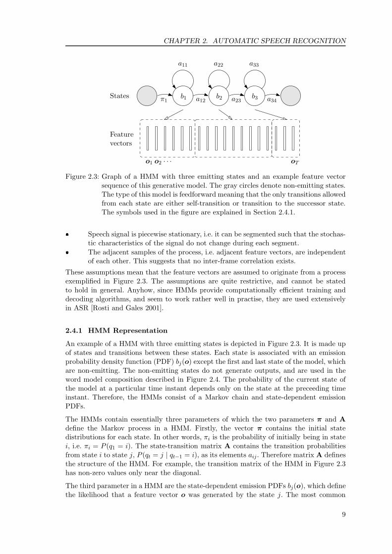
Figure 2.3: Graph of a HMM with three emitting states and an example feature vectorsequence of this generative model. The gray circles denote non-emitting states.The type of this model is feedforward meaning that the only transitions allowedfrom each state are either self-transition or transition to the successor state.The symbols used in the figure are explained in Section 2.4.1.
� Speech signal is piecewise stationary, i.e. it can be segmented such that the stochas-tic characteristics of the signal do not change during each segment.
� The adjacent samples of the process, i.e. adjacent feature vectors, are independentof each other. This suggests that no inter-frame correlation exists.
These assumptions mean that the feature vectors are assumed to originate from a processexemplified in Figure 2.3. The assumptions are quite restrictive, and cannot be statedto hold in general. Anyhow, since HMMs provide computationally efficient training anddecoding algorithms, and seem to work rather well in practise, they are used extensivelyin ASR [Rosti and Gales 2001].
2.4.1 HMM Representation
An example of a HMM with three emitting states is depicted in Figure 2.3. It is made upof states and transitions between these states. Each state is associated with an emissionprobability density function (PDF) bj(o) except the first and last state of the model, whichare non-emitting. The non-emitting states do not generate outputs, and are used in theword model composition described in Figure 2.4. The probability of the current state ofthe model at a particular time instant depends only on the state at the preceeding timeinstant. Therefore, the HMMs consist of a Markov chain and state-dependent emissionPDFs.
The HMMs contain essentially three parameters of which the two parameters π and Adefine the Markov process in a HMM. Firstly, the vector π contains the initial statedistributions for each state. In other words, πi is the probability of initially being in statei, i.e. πi = P (q1 = i). The state-transition matrix A contains the transition probabilitiesfrom state i to state j, P (qt = j | qt−1 = i), as its elements aij . Therefore matrix A definesthe structure of the HMM. For example, the transition matrix of the HMM in Figure 2.3has non-zero values only near the diagonal.
The third parameter in a HMM are the state-dependent emission PDFs bj(o), which definethe likelihood that a feature vector o was generated by the state j. The most common
9
CHAPTER 2. AUTOMATIC SPEECH RECOGNITION
case is that these emission PDFs are continuous and of mixture type, i.e.
bj(o) =Mj∑k=1
wjkfD(o; θjk) (2.7)
where Mj is the number of mixture components, and wjk the weight of the k:th mix-ture component density of the state j. The mixture component weights must satisfy thecondition
Mj∑i=1
wji = 1 with wjk ≥ 0 ∀j, k (2.8)
in order bj(o) to fulfill the properties of a PDF [Bishop 1998]. The component densi-ties fD(o; θjk) are density functions of some known distributions D with parameters θjk.Most often fD(o; θ) is the multivariate Gaussian density function defined as [Johnson andWichern 1998]
fN (o;µ,Σ) =1
(2π)D/2√|Σ| exp
[(o − µ)TΣ−1(o − µ)
](2.9)
where θ consists of µ, the mean, and Σ, the covariance matrix of the distribution. In thatcase, the density in Equation (2.7) is also known as Gaussian mixture model (GMM).Furthermore, the covariance matrices of the Gaussian distributions are often constraineddiagonal. Diagonality of the covariance matrices reduces the total number of parameters inthe model significantly, especially when the dimension of the feature vector is large. Eventhough the diagonality of the covariance matrix of a component density suggests that theelements of the modeled random vector are independent5, the mixture of these densitiesbj(o) can model correlation characteristics as well [Reynolds et al. 2000]. In addition,different parameter tying schemes have been proposed for covariance matrix modeling inHMMs, e.g. semi-tied covariance matrices [Gales 1999].
Alternative types of observation emission densities than the usual GMMs have beenproposed for ASR applications, e.g. Richter, power exponential and Laplacian distribu-tions [Gales and Olsen 1999]. However, no significant advantages have been achieved byusing these different observation densities. The parameters of all the state-dependent emis-sion densities in a HMM are denoted with Θ. For the clarity of notation, we use a singlesymbol λ = (π,A,Θ) to denote the whole parameter set of a single HMM. In Chapter 4,both symbols λ and κ are used to denote this parameter set.
2.4.2 Speech Recognition Using HMMs
In order to solve the classification task defined in Equation (2.6), the likelihood P (O | λW )and prior probability P (λW ) need to be determined for each word model λW .
The usual case is that the acoustic units, that are modeled as single HMMs, representphonemes. In this case, the word models λW must be constructed before recognition. Thisword model composition is depicted in Figure 2.4. First of all, the phonetic transcriptionof the current word is obtained from the lexicon. Then, the corresponding phoneme modelsare concatenated after each other to form a single word model. This procedure is appliedto all the vocabulary items. In the following, the evaluation of P (O | λW ) is determined
10

CHAPTER 2. AUTOMATIC SPEECH RECOGNITION
/s/ /t/
/�//p/
Figure 2.4: Concatenation of HMMs. The phonetic transcription of the english word“stop”written using IPA symbols is /st�p/. The word consists of four phonemes,which are modeled using separate phoneme models. These monophone HMMscorresponding to the phonemes are concatenated using the non-emitting statesin the beginning and at the end of the models. By defining the symbol “⊕” toindicate the model concatenation, the model for the word“stop”can be writtenas /s/⊕/t/⊕/�/⊕/p/.
for only one HMM. The evaluation of P (O | λW ) for concatenated HMMs can be founde.g. in [Jelinek 1998].
The likelihood of a feature vector sequence O given a HMM with parameters λ can becalculated as follows [Rabiner 1993]
P (O | λ) =∑
�∈Q(T )
P (O,q | λ) =∑
�∈Q(T )
πq1
T−1∏t=1
bqt(ot)aqtqt+1 (2.10)
where Q(T ) is the set of all state sequences of length T . Usually, when the last observationvector is encountered, the state is restricted to be the last non-emitting state of the model,in which case
Q(T ) ={q ∈ �T : qT = N
}(2.11)
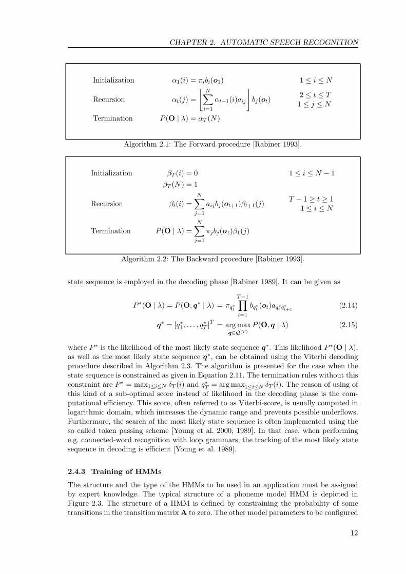
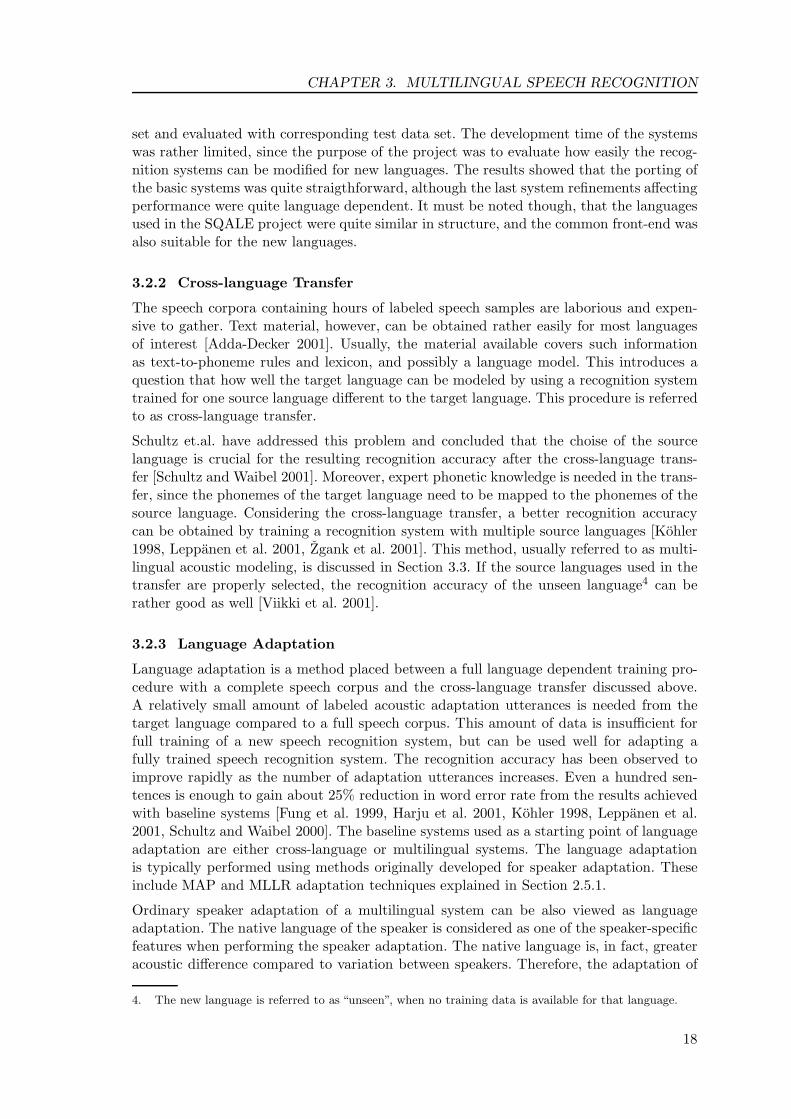
where N is the number of states in the model. The Equation (2.10) can be evaluatedrecursively using the forward or backward procedure explained in Algorithms 2.1 and 2.2,respectively [Rabiner 1993]. The forward and backward variables αt(j) and βt(j) are de-fined as [Rabiner 1993]
αt(j) = P (o1,o2, · · · ,ot, qt = j | λ) (2.12)βt(j) = P (ot+1,ot+2, · · · ,oT | qt = j, λ) (2.13)
The constraint qT = N results in the termination rule in Algorithm 2.1. In the literature,the termination rule is determined without this constraint, i.e. P (O | λ) =
∑Ni=1 αT (i) [Ra-
biner 1993]. Similarly, the initialization rule in Algorithm 2.2 can be given as βT (i) = 1, 1 ≤i ≤ N without the constraint qT = N .
Often, instead of using the likelihood in Equation (2.10), the likelihood of the most likely
5. In the case of Gaussian distributions, uncorrelatedness of the elements is equivalent with their inde-pendence [Johnson and Wichern 1998].
11
CHAPTER 2. AUTOMATIC SPEECH RECOGNITION
Initialization α1(i) = πibi(o1) 1 ≤ i ≤ N
Recursion αt(j) =
[N∑
i=1
αt−1(i)aij
]bj(ot)
2 ≤ t ≤ T1 ≤ j ≤ N
Termination P (O | λ) = αT (N)
Algorithm 2.1: The Forward procedure [Rabiner 1993].
Initialization βT (i) = 0 1 ≤ i ≤ N − 1βT (N) = 1
Recursion βt(i) =N∑
j=1
aijbj(ot+1)βt+1(j)T − 1 ≥ t ≥ 1
1 ≤ i ≤ N
Termination P (O | λ) =N∑
j=1
πjbj(o1)β1(j)
Algorithm 2.2: The Backward procedure [Rabiner 1993].
state sequence is employed in the decoding phase [Rabiner 1989]. It can be given as
P ∗(O | λ) = P (O,q∗ | λ) = πq∗1
T−1∏t=1
bq∗t (ot)aq∗t q∗t+1(2.14)
q∗ = [q∗1, . . . , q∗T ]T = arg max
�∈Q(T )
P (O,q | λ) (2.15)
where P ∗ is the likelihood of the most likely state sequence q∗. This likelihood P ∗(O | λ),as well as the most likely state sequence q∗, can be obtained using the Viterbi decodingprocedure described in Algorithm 2.3. The algorithm is presented for the case when thestate sequence is constrained as given in Equation 2.11. The termination rules without thisconstraint are P ∗ = max1≤i≤N δT (i) and q∗T = arg max1≤i≤N δT (i). The reason of using ofthis kind of a sub-optimal score instead of likelihood in the decoding phase is the com-putational efficiency. This score, often referred to as Viterbi-score, is usually computed inlogarithmic domain, which increases the dynamic range and prevents possible underflows.Furthermore, the search of the most likely state sequence is often implemented using theso called token passing scheme [Young et al. 2000; 1989]. In that case, when performinge.g. connected-word recognition with loop grammars, the tracking of the most likely statesequence in decoding is efficient [Young et al. 1989].
2.4.3 Training of HMMs
The structure and the type of the HMMs to be used in an application must be assignedby expert knowledge. The typical structure of a phoneme model HMM is depicted inFigure 2.3. The structure of a HMM is defined by constraining the probability of sometransitions in the transition matrix A to zero. The other model parameters to be configured
12

CHAPTER 2. AUTOMATIC SPEECH RECOGNITION
Initialization δ1(j) = πjbj(o1) 1 ≤ j ≤ N
ψ1(j)Recursion δt(j) = max
1≤i≤N[δt−1(i)aij ]bj(ot) 2 ≤ t ≤ T
ψt(j) = arg max1≤i≤N
δt−1(i)aij 1 ≤ j ≤ N
Termination P ∗ = δT (N)q∗T = N
Path backtracking q∗t = ψt+1(q∗t+1) t = T − 1, T − 2, . . . , 1
Algorithm 2.3: The Viterbi decoding algorithm [Viterbi 1967]. Temporary variables ψt(i)and δt(i) contain the information of the most likely state sequence up tothe state i at time instant t. The index of the previous state is stored inψt(i) while δt(i) contains the accumulated likelihood.
include the type of mixture densities, the number of the mixture component densities in thestate-dependent emission denisities and the number of states in one HMM. Furthermore,the acoustic units to be modeled with a single HMM must be fixed.
After defining the configuration of HMMs, the parameters should be estimated using somemethod. Typically, these parameters are estimated using a labeled speech corpus contain-ing a huge amount of training utterances. Assuming that monophone models are used,i.e. every phoneme is modeled with a single HMM, a combined word model is created tocorrespond to the phonetic transcription of each train utterance. The model concatenationscheme used in word model composition is shown in Figure 2.4. The training procedureusing the combined word models is also referred to as the embedded re-estimation of theparameters [Young et al. 2000].
Most often the parameters are estimated according to the maximum-likelihood criterion.The expectation-maximization (EM) algorithm provides an iterative procedure for esti-mating the maximum likelihood estimates (MLEs) of the parameters λ of a HMM. Ateach iteration of the EM algorithm, the value of the likelihood function increases, converg-ing to a local MLE of λ [Dempster et al. 1977]. For the sake of clarity, this algorithm ispresented in the following for a single observation sequence. The generalization of the al-gorithm to multiple observation sequences as well as detailed description of the derivationof the following re-estimation equations can be found e.g. in [Rabiner 1993].
At each iteration of the EM algorithm for HMMs, the Baum’s auxiliary function givenas [Baum 1972]
Q(λ, λ) =∑�∈Q
P (q | O, λ) log P (O,q | λ) (2.16)
is maximized with respect to the new HMM parameter estimates λ. The detailed descrip-tion of this maximization procedure can be found e.g. in [Rabiner 1993]. The maximizationof Q results in an increased value of the likelihood function,
λ = arg max�λ
Q(λ, λ) =⇒ P (O | λ) ≥ P (O | λ) (2.17)
13

CHAPTER 2. AUTOMATIC SPEECH RECOGNITION
The new estimates of the parameters λ are given in the following Baum-Welch re-estimationformulae [Rabiner 1993]. The given formulae apply for HMMs with GMM emission densi-ties.
πi = γ1(i) (2.18)
aij =∑T−1
t=1 ξt(i, j)∑T−1t=1
∑Ml=1 γt(j, l)
(2.19)
wjk =∑T
t=1 γt(j, k)∑Tt=1
∑Ml=1 γt(j, l)
(2.20)
µjk =∑T
t=1 γt(j, k) · ot∑Tt=1 γt(j, k)
(2.21)
Σjk =
∑Tt=1 γt(j, k) · (ot − µjk)(ot − µjk)T∑T
t=1 γt(j, k)(2.22)
The symbols on the left hand side of the Equations (2.18)–(2.22) are the new estimatesof the parameters λ explained in Section 2.4.1. The auxiliary variables used in Equations(2.18)–(2.22) are defined as ξt(i, j) = P (qt = i, qt+1 = j | O, λ) and γt(j, k) = P (qt =j,mixture component = k | O, λ). The latter is often referred as the a posteriori probabilityof the tth observation being emitted from the kth mixture of state j. They can be obtainedas follows [Rabiner 1993]
ξt(i, j) =αt(i)aijbj(ot+1)βt+1(j)∑N
i=1
∑Nj=1 αt(i)aijbj(ot+1)βt+1(j)
(2.23)
γt(j, k) =
[αt(j)βt(j)∑N
j=1 αt(j)βt(j)
][wjkfN (ot;µjk,Σjk)
bj(ot)
](2.24)
where fN (·;µ,Σ) denotes the multivariate Gaussian density function. The forward andbackward variables, αt(j) and βt(j), respectively, used in the formulae are obtained fromthe procedures in Algortihms 2.1 and 2.2.
2.5 Speaker Adaptation
The estimation of the parameters of the statistical models used in a speech recognitionsystem demands large amounts (hours) of speech material. Training a speaker independent(SI) speech recognition system is straightforward due to large annotated speech databasesavailable. The SI recognition systems perform rather well in most cases, but the errorrate is two to three times higher than with speaker dependent (SD) systems [Leggetterand Woodland 1994]. The SD recognition system provides better modeling of the speechcharacteristics for the target speaker. However, it is unfeasible to gather such a largeamount of speech material for every speaker. Model adaptation techniques provide methodsfor adapting a SI recognition system for the target speaker using only small amount ofacoustic adaptation material. A notable gain in recognition accuracy is achieved by theuse of such techniques [Leggetter and Woodland 1994].
Often, speaker adaptation is performed using maximum a posteriori (MAP) or maximumlikelihood linear regression (MLLR) methods, which both are model adaptation techniques.
14

CHAPTER 2. AUTOMATIC SPEECH RECOGNITION
The maximum a posteriori (MAP) technique provides a method for adapting the param-eters of the HMMs with a relatively small amount of adaptation data per model [Gau-vain and Lee 1994]. HMMs without adaptation data are left unchanged. Alternatively,the maximum likelihood linear regression (MLLR) can be employed for speaker adapta-tion [Leggetter and Woodland 1994]. This method is useful particularly when context-dependent models6, are used in the speech recognition system. In the MLLR framework,all the HMMs are adapted, even such HMMs that do not have any adaptation data. Thisis achieved such that the mixture density components of the HMM states are allocatedto so called transformation classes, which share the adaptation data of all the densities insuch class. The transformation classes are formed using the acoustic similarities betweenthe models. The MLLR technique is presented in brief in the following for HMMs withGMM emission densities.
2.5.1 Maximum Likelihood Linear Regression
The MLLR technique is based on an affine transformation of the mean vectors µ ∈ �D
for each mixture component. The transformation is defined as [Leggetter and Woodland1994]
µ = Wν = W[ωµ
](2.25)
where µ is the new (transformed) mean vector, W ∈ �D×(D+1) is the transformation
matrix and ω is the offset term for the regression.
The transformation matrix W is derived via similar optimization scheme as in the Baum-Welch training procedure described in Section 2.4.3. The optimization scheme results inthat the transformation matrix WΓ can be obtained for the mixture components in trans-formation class Γ by solving [Leggetter and Woodland 1994]
∑(j,k)∈Γ
T∑t=1
γt(j, k)Σ−1jk otν
Tjk =
∑(j,k)∈Γ
T∑t=1
γt(j, k)Σ−1jk WΓνjkν
Tjk (2.26)
where the a posteriori probabilities γt(j, k) are described in Section 2.4.3. The outer sums inEquation (2.26) go through all the mixture density components i.e. corresponding (state,mixture) pairs. The matrix WΓ can be solved from Equation (2.26) with the essentialcost of D matrix inversions of dimension D + 1, where D is the dimension of the featurevector [Leggetter and Woodland 1994]. The determination of the transformation classesΓ is discussed in Appendix A. These classes can be determined using the dissimilaritymeasures explained in Chapter 4, but the topic is beyond the scope of this thesis.
6. The widely used context-dependent phone models in ASR are the so called triphone models. Theyhave explicit left and right context phones. The number of unique triphone models is p3, where p is thenumber of unique phonemes in the language. Typically p is around 40.
15

Chapter 3
Multilingual Speech Recognition
The research in the field of speech recognition has been rather intense on few major lan-guages, namely on the American English [Adda-Decker 2001, Young et al. 1997]. Manypotential applications, however, require support for multiple languages. These includee.g. voice dialing applications in mobile handsets, which are typically aimed for widegeographic areas covering numerous languages [Kiss 2001]. Even the support for minorlanguages can be considered a necessity in these kind of applications. The flight reserva-tion systems are another area of applications which benefit from the support of multiplelanguages, non-native speakers and speakers with strong dialects. The benefits of a mul-tilingual ASR system include also reduced development costs, as no different languagedependent versions of the system need to be developed [Viikki et al. 2001].
The main topics in the field of multilingual speech recognition are the porting of existingrecognition systems for new languages and the multilingual acoustic modeling. The latterconcerns the development of a multilingual recognition system without separate acousticmodels for each language. The porting covers development of a speech recognition systemfor new language using existing speech recognition systems and corpora. The issue ofmultilinguality in speech recognition is still fairly new. The first publications concerningmultilinguality in speech technology are from the late 1980s. However, from the middle ofthe 1990s, this research are has started to gain increasing attention [Adda-Decker 2001,Andersen et al. 1994, Byrne et al. 2000, Fung et al. 1999, Imperl and Horvat 1999, Kiss2001, Kohler 2001, Navratil 2001, Uebler 2001, Van Compernolle 2001, Waibel et al. 2000,Young et al. 1997].
This chapter covers the issues of multilingual ASR discussed above. The Section 3.1 re-views the most basic resources, speech corpora needed for the development purposes ofmultilingual speech recognition. Next, in Section 3.2, the portability of ASR technology isdiscussed. The Section 3.3 covers the issues of multilingual acoustic modeling.
3.1 Multilingual Speech Corpora
The labeled speech corpora are the basic resources needed in the development of speechrecognition systems. Considering multilingual speech recognition systems, extra require-ments are set on the speech corpora. The corpora must include several language dependentspeech corpora compatible to each other. This means that the acoustic conditions, such asbackground noise and microphone distortions, should be similar. Furthermore, the contentof speech, i.e. the vocabulary and the type of speech should be similar. The training andtest sets should also be similar to achieve comparable results across the languages.
16

CHAPTER 3. MULTILINGUAL SPEECH RECOGNITION
As the research in multilingual ASR has gained momentum, a number of multilingualspeech corpora have been introduced [Adda-Decker 2001]. These include SpeechDat, OGI,LDC CallHome1 and GlobalPhone [Muthusamy et al. 1992, Schultz et al. 1997, Winski1997].
3.2 Portability of Speech Technology
Since most of the technology used in modern ASR applications is developed for a singlelanguage we can ask what are the parts of the speech recognition systems2 that canbe considered language independent. Furthermore, can the same development methodsexplained in Section 2.4 be used for training a speech recognition system for any languageprovided that a suitable speech corpus exists? For many minor languages, such corpusdoes not exists, and the collection of such a large database is unfeasible. In such a case,is it possible to obtain a speech recognition system for a new language with no acousticdata, or very little acoustic data available? The following sections cover these issues.
3.2.1 Language-dependency of Speech Recognition Systems
The typical MFCC feature extraction unit explained in Section 2.3 can be considered rela-tively language-independent, because only low-level signal processing is performed at thatlevel [Adda-Decker 2001, Kiss 2001]. The acoustic features commonly used in recognitionof the English language can be used also in recognition of e.g. most of the other Europeanlanguages. These acoustic features do not include information of pitch, which is vital whenrecognizing tonal languages, e.g. Mandarin Chinese. In such languages, the whole meaningof a phrase can change due to different pitch pattern [Lee 1997]. A modified front-endcan be formed where the feature vector is augmented to comprise also information ofpitch [Chang et al. 2000].
The acoustic models used in modern speech recognition systems are HMMs, as explainedin Section 2.4.1. The training as well as the decoding algorithms of HMMs are general, andindependent of the language [Adda-Decker 2001]. However, the topology of the HMMs andthe decision of the acoustic units3 to be modeled with a single HMM can demand languagedependent research. Therefore, the framework of acoustic modeling is applicable in generalwithout modifications, regardless of the language.
The lexicon and the language model are obviously the most language dependent partsof the system. The languages are very different in both written and spoken form. Thesegmentation into words, morphology and the used character set differs greatly betweenlanguages. The morphology and prosody reflect to the spoken form of the language [Waibelet al. 2000]. Most European languages seem to share many common features, but whencomparing e.g. Asian languages to European languages, the differences are tremendous.
The porting of the existing speech recognition systems was researched in the EuropeanSQALE project [Young et al. 1997]. Four recognition systems designed originally for Amer-ican English were compared in recognition of three European languages: British English,French and German. The systems were trained using a common predefined training data
1. See Linguistic Data Consortium (LDC), University of Pennsylvania web page for details:http://www.ldc.upenn.edu.2. The structure of modern ASR system is depicted in Figure 2.1.3. The acoustic unit refers here to phoneme, allophone or syllable.
17
CHAPTER 3. MULTILINGUAL SPEECH RECOGNITION
set and evaluated with corresponding test data set. The development time of the systemswas rather limited, since the purpose of the project was to evaluate how easily the recog-nition systems can be modified for new languages. The results showed that the porting ofthe basic systems was quite straigthforward, although the last system refinements affectingperformance were quite language dependent. It must be noted though, that the languagesused in the SQALE project were quite similar in structure, and the common front-end wasalso suitable for the new languages.
3.2.2 Cross-language Transfer
The speech corpora containing hours of labeled speech samples are laborious and expen-sive to gather. Text material, however, can be obtained rather easily for most languagesof interest [Adda-Decker 2001]. Usually, the material available covers such informationas text-to-phoneme rules and lexicon, and possibly a language model. This introduces aquestion that how well the target language can be modeled by using a recognition systemtrained for one source language different to the target language. This procedure is referredto as cross-language transfer.
Schultz et.al. have addressed this problem and concluded that the choise of the sourcelanguage is crucial for the resulting recognition accuracy after the cross-language trans-fer [Schultz and Waibel 2001]. Moreover, expert phonetic knowledge is needed in the trans-fer, since the phonemes of the target language need to be mapped to the phonemes of thesource language. Considering the cross-language transfer, a better recognition accuracycan be obtained by training a recognition system with multiple source languages [Kohler1998, Leppanen et al. 2001, Zgank et al. 2001]. This method, usually referred to as multi-lingual acoustic modeling, is discussed in Section 3.3. If the source languages used in thetransfer are properly selected, the recognition accuracy of the unseen language4 can berather good as well [Viikki et al. 2001].
3.2.3 Language Adaptation
Language adaptation is a method placed between a full language dependent training pro-cedure with a complete speech corpus and the cross-language transfer discussed above.A relatively small amount of labeled acoustic adaptation utterances is needed from thetarget language compared to a full speech corpus. This amount of data is insufficient forfull training of a new speech recognition system, but can be used well for adapting afully trained speech recognition system. The recognition accuracy has been observed toimprove rapidly as the number of adaptation utterances increases. Even a hundred sen-tences is enough to gain about 25% reduction in word error rate from the results achievedwith baseline systems [Fung et al. 1999, Harju et al. 2001, Kohler 1998, Leppanen et al.2001, Schultz and Waibel 2000]. The baseline systems used as a starting point of languageadaptation are either cross-language or multilingual systems. The language adaptationis typically performed using methods originally developed for speaker adaptation. Theseinclude MAP and MLLR adaptation techniques explained in Section 2.5.1.
Ordinary speaker adaptation of a multilingual system can be also viewed as languageadaptation. The native language of the speaker is considered as one of the speaker-specificfeatures when performing the speaker adaptation. The native language is, in fact, greateracoustic difference compared to variation between speakers. Therefore, the adaptation of
4. The new language is referred to as “unseen”, when no training data is available for that language.
18

CHAPTER 3. MULTILINGUAL SPEECH RECOGNITION
language-specific features is a big part of the speaker adaptation that is performed formultilingual ASR systems [Viikki et al. 2001].
3.3 Multilingual Acoustic Modeling
The concept of a phonetic typewriter issued in the 1950s was based on the idea of a machinecapable of transcribing auditory speech signals [Gold and Morgan 2000]. The sound units inspoken languages, phonemes, were supposed to be distinguishable from spoken utterances,which could be then transferred e.g. to a written form. This showed to be inapplicablesince the variation of the phonemes differs greatly according to context, speaking style,age, and the language used. Even a human listener cannot transcribe spoken utterancesreliably if the linguistic content is unclear. This is also the situation when the listener isunfamiliar with the language.
All the spoken languages still do seem to share common acoustic features. The source ofspeech, i.e. the human speech production system, is the same regardless of the languageused. This implies that the speech signals share common acoustic features, originatingfrom the physical properties of the human speech production system. In all the spokenlanguages, the content of speech is determined by a stream of phonemes articulated aftereach other. Thus the use of left-to-right proceeding HMMs as acoustic models can beconsidered a language independent strategy for acoustic modeling in speech recognitionapplications. The multilingual acoustic modeling can be stated applicable based on thesefacts.
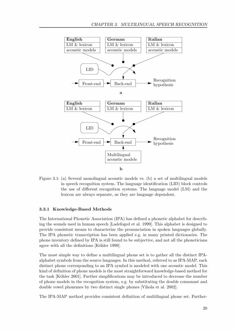
The Figure 3.1 shows how the sharing of acoustic models across languages effects thestructure of a speech recognition system. Instead of using a separate set of acoustic modelsfor each language, a common set of models is utilized in multilingual acoustic modeling.This results in the following benefits. The development costs are reduced as there is noneed developing separate language dependent systems [Viikki et al. 2001]. In addition, themultilingual systems can cope with non-native speakers, accents, dialects and multilingualvocabulary items [Viikki et al. 2001].
Even when constructing a language dependent speech recognition system, the model pa-rameters can be shared5 [Woodland and Young 1993]. The reasons for this are twofold.Firstly, such units that are unseen in the training phase can share the parameters of otherunits. Secondly, the number of free parameters in a speech recognition system can be re-duced without notable drop in recognition accuracy [Woodland and Young 1993]. In fact,when the number of free parameters is lower, the statistical estimation of the parameters ismore robust, which can improve the performance and generality of the speech recognitionsystem [Woodland and Young 1993]. The research concerning multilingual acoustic mod-eling indicated that much can be gained by modeling different languages with commonacoustic models. The following sections outline the methods for developing multilingualspeech recognition systems. The Sections 3.3.1 and 3.3.2 describe the knowledge-based andcomputational approaches for the definition of a set of multilingual acoustic models. TheSection 3.3.3 outlines the functionality of the language identification (LID) unit needed ina multilingual ASR system.
5. This is performed most often with ASR systems having context-dependent acoustic units, e.g. triphoneHMMs.
19
CHAPTER 3. MULTILINGUAL SPEECH RECOGNITION
LID
LID
Multilingual
Front-end
Front-end
Back-end
Back-end
Recognition
Recognition
hypothesis
hypothesis
b
a
acoustic models acoustic modelsacoustic models
acoustic models
German
German
Italian
Italian
English
English
LM & lexiconLM & lexiconLM & lexicon
LM & lexiconLM & lexiconLM & lexicon
Figure 3.1: (a) Several monolingual acoustic models vs. (b) a set of multilingual modelsin speech recognition system. The language identification (LID) block controlsthe use of different recognition systems. The language model (LM) and thelexicon are always separate, as they are language dependent.
3.3.1 Knowledge-Based Methods
The International Phonetic Association (IPA) has defined a phonetic alphabet for describ-ing the sounds used in human speech [Ladefoged et al. 1999]. This alphabet is designed toprovide consistent means to characterize the pronunciation in spoken languages globally.The IPA phonetic transcription has been applied e.g. in many printed dictionaries. Thephone inventory defined by IPA is still found to be subjective, and not all the phoneticiansagree with all the definitions [Kohler 1999].
The most simple way to define a multilingual phone set is to gather all the distinct IPA-alphabet symbols from the source languages. In this method, referred to as IPA-MAP, eachdistinct phone corresponding to an IPA symbol is modeled with one acoustic model. Thiskind of definition of phone models is the most straightforward knowledge-based method forthe task [Kohler 2001]. Further simplifications may be introduced to decrease the numberof phone models in the recognition system, e.g. by substituting the double consonant anddouble vowel phonemes by two distinct single phones [Vihola et al. 2002].
The IPA-MAP method provides consistent definition of multilingual phone set. Further-
20

CHAPTER 3. MULTILINGUAL SPEECH RECOGNITION
more, if a set of multilingual acoustic models is created according to the IPA alphabet6,the recognition system should be potentially language independent. This means that anunseen target language can be recognized if the phone inventory of the source languagesis sufficient, i.e. it contains all the phonemes in the target language. The IPA chart isdefined for the purposes of the phonetic representation of the languages, and is based onarticulatory features of the sounds. It may not describe the acoustic features as accuratelyas is needed for the purposes of speech recognition, e.g. the representation does not coverthe allophone variation of one phoneme.
3.3.2 Computational Methods
When expert knowledge is not available or, e.g. the number of multilingual phone modelsis constrained to be very low, the IPA-MAP method may not be useful. In this case, anautomatic, i.e. computational, method may provide an alternative approach for defining aset of multilingual phone models [Kohler 2001]. Using the same number of phone modelsas in the IPA-MAP method, the recognition accuracy of the resulting multilingual ASRsystem has been observed to be slightly better with the computational method [Kohler2001]. Conversely, a recognition accuracy comparable to the IPA-MAP recognition systemcan be achieved with less phone models when using the computational method [Harjuet al. 2001].
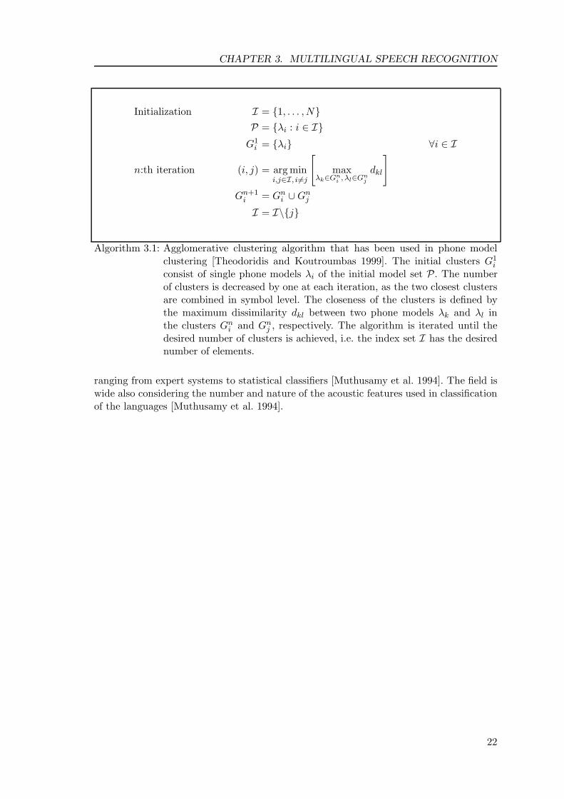
The computational methods used in defining the multilingual phone model set are based onsome measure of dissimilarity of two language dependent phoneme models, namely HMMs.These dissimilarity measures are reviewed and described in detail in Chapter 4. Usually,this kind of a measure is employed, and the models are collected to certain number of clus-ters, and each cluster is modeled with a common multilingual phone model. The clustersare typically obtained using a bottom-up, i.e. agglomerative clustering algorithm [Harjuet al. 2001, Kohler 2001]. This algorithm is described briefly in Algorithm 3.1.
3.3.3 Language Identification
A multilingual speech recognition system is fully operational after a language identification(LID) block is implemented [Kiss 2001]. The decision in LID block is made accordingto some knowledge about the spoken language. The knowledge of the language can beexplicit, e.g. defined by the user, or automatically identified. The function of the LIDblock in the recognition system is depicted in Figure 3.1. In the case of multilingualrecognition system constructed from a set of monolingual recognition systems, the LIDblock switches between the monolingual recognition systems as shown in Figure 3.1 (a).After the language selection, the recognition system performs the recognition using thechosen monolingual system. In the case of a multilingual recognition system with commonmultilingual acoustic models only the language model and the lexicon need to be selected.The same acoustic models are used for all the languages. This is shown in Figure 3.1 (b).
Automatic language identification has many real-world applications including telephonyservices, such as hotel reservation and emergency lines [Muthusamy et al. 1994]. The issueof language identification has been researched for decades, and it seems that the peakin the number of published reports and articles is just before middle of the 1990s. Thesystems implemented for language identification purposes are based on numerous methods
6. Usually, the alphabet used in computer environments is Speech Assessment Methods Phonetic Alpha-bet, SAMPA. It is a mapping of IPA alphabet into ASCII codes [SAM].
21
CHAPTER 3. MULTILINGUAL SPEECH RECOGNITION
Initialization I = {1, . . . , N}P = {λi : i ∈ I}G1
i = {λi} ∀i ∈ I
n:th iteration (i, j) = arg mini,j∈I, i�=j
[max
λk∈Gni , λl∈Gn
j
dkl
]Gn+1
i = Gni ∪Gn
j
I = I\{j}
Algorithm 3.1: Agglomerative clustering algorithm that has been used in phone modelclustering [Theodoridis and Koutroumbas 1999]. The initial clusters G1
i
consist of single phone models λi of the initial model set P. The numberof clusters is decreased by one at each iteration, as the two closest clustersare combined in symbol level. The closeness of the clusters is defined bythe maximum dissimilarity dkl between two phone models λk and λl inthe clusters Gn
i and Gnj , respectively. The algorithm is iterated until the
desired number of clusters is achieved, i.e. the index set I has the desirednumber of elements.
ranging from expert systems to statistical classifiers [Muthusamy et al. 1994]. The field iswide also considering the number and nature of the acoustic features used in classificationof the languages [Muthusamy et al. 1994].
22
Chapter 4
Dissimilarity Measures for Hidden Markov Models
In Chapter 3, the concept of multilingual acoustic modeling was discussed. The Sec-tion 3.3.2 summarized the computational method used in definition of a set of multilingualphone models. The explained method was based on a dissimilarity measurement of the LDphoneme models, i.e. HMMs. This dissimilarity has been evaluated in the previous researchprojects using one of the two methods: the Kullback-Leibler (KL) divergence estimate, oran estimate based on the confusion matrix [Andersen et al. 1994, Harju et al. 2001, Kohler2001]. Both of the estimates have been obtained using some speech data set. However,these methods have mainly two drawbacks: Firstly, the estimation procedure is computa-tionally expensive. Secondly, as the measures have been obtained from statistics computedusing some speech data set1, these measures have a considerable variation to the case whenthe measures are evaluated from another data set.
This chapter reviews the dissimilarity measures for HMMs. In addition to the above men-tioned computational phoneme model clustering, the dissimilarity measures can be utilizedin speech recognition e.g. in model selection and clustering [Juang and Rabiner 1985]. Fur-thermore, the measures could be applied in the MLLR adaptation framework, as describedin Appendix A. A detailed description of such dissimilarity measures that are suitable forthe purposes of phoneme model clustering is given in this chapter. Although these measuresare presented only for the monophone HMMs, most of the techinques can be generalizedfor cases in which different acoustic modeling units, e.g. allophones or words, are used. Inaddition, it should be noted that all the measures described in this chapter are consideredas dissimilarity measures. This is due to simpler representation, interpretation and compar-ison of the measures. Intuitively, a dissimilarity measure can be considered as a “distance”metric. All the dissimilarity measures described in this chapter, however, do not fulfill theproperties of a proper metric2. Therefore, the presented measures are generally referred toas dissimilarity measures.
The natural criterion, that describes the dissimilarity of statistical models used in pat-tern recognition, is the classification characteristics, i.e. the nature of the errors made inclassification task. This can be measured e.g. using a confusion matrix such as shown inTable 4.1. An interpretation of the dissimilarity in such a case is as follows. The more
1. This means that the speech data is considered as independent random observations of the HMMs.2. In topology, a metric is a function that describes proximity of objects. It is defined formally as afunction d : X × X → [0,∞), having the following properties:
1. d(x, y) = 0 if and only if x = y2. d(x, y) = d(y, x)3. d(x, z) ≤ d(x, y) + d(y, z)
where x, y and z are elements of the topological space X [Gariepy and Ziemer 1994].
23
CHAPTER 4. DISSIMILARITY MEASURES FOR HMMS
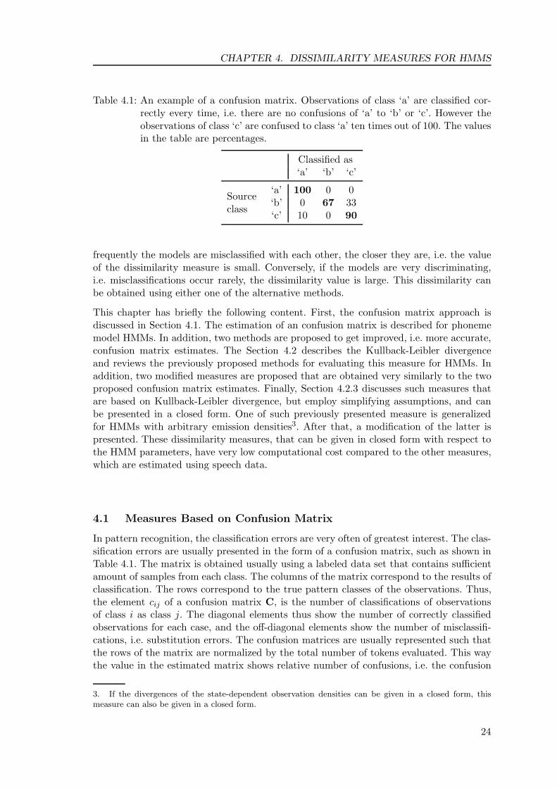
Table 4.1: An example of a confusion matrix. Observations of class ‘a’ are classified cor-rectly every time, i.e. there are no confusions of ‘a’ to ‘b’ or ‘c’. However theobservations of class ‘c’ are confused to class ‘a’ ten times out of 100. The valuesin the table are percentages.
Classified as‘a’ ‘b’ ‘c’
Sourceclass
‘a’ 100 0 0‘b’ 0 67 33‘c’ 10 0 90
frequently the models are misclassified with each other, the closer they are, i.e. the valueof the dissimilarity measure is small. Conversely, if the models are very discriminating,i.e. misclassifications occur rarely, the dissimilarity value is large. This dissimilarity canbe obtained using either one of the alternative methods.
This chapter has briefly the following content. First, the confusion matrix approach isdiscussed in Section 4.1. The estimation of an confusion matrix is described for phonememodel HMMs. In addition, two methods are proposed to get improved, i.e. more accurate,confusion matrix estimates. The Section 4.2 describes the Kullback-Leibler divergenceand reviews the previously proposed methods for evaluating this measure for HMMs. Inaddition, two modified measures are proposed that are obtained very similarly to the twoproposed confusion matrix estimates. Finally, Section 4.2.3 discusses such measures thatare based on Kullback-Leibler divergence, but employ simplifying assumptions, and canbe presented in a closed form. One of such previously presented measure is generalizedfor HMMs with arbitrary emission densities3. After that, a modification of the latter ispresented. These dissimilarity measures, that can be given in closed form with respect tothe HMM parameters, have very low computational cost compared to the other measures,which are estimated using speech data.
4.1 Measures Based on Confusion Matrix
In pattern recognition, the classification errors are very often of greatest interest. The clas-sification errors are usually presented in the form of a confusion matrix, such as shown inTable 4.1. The matrix is obtained usually using a labeled data set that contains sufficientamount of samples from each class. The columns of the matrix correspond to the results ofclassification. The rows correspond to the true pattern classes of the observations. Thus,the element cij of a confusion matrix C, is the number of classifications of observationsof class i as class j. The diagonal elements thus show the number of correctly classifiedobservations for each case, and the off-diagonal elements show the number of misclassifi-cations, i.e. substitution errors. The confusion matrices are usually represented such thatthe rows of the matrix are normalized by the total number of tokens evaluated. This waythe value in the estimated matrix shows relative number of confusions, i.e. the confusion
3. If the divergences of the state-dependent observation densities can be given in a closed form, thismeasure can also be given in a closed form.
24

CHAPTER 4. DISSIMILARITY MEASURES FOR HMMS
frequency, which can be given as
cij =card {k : Oκi
k is classified as κj}card {k : Oκi
k } (4.1)
where card denotes the number of elements in the set. Once a confusion matrix estimateC is obtained for the set of models, it contains the estimates of how likely it is that agiven model is classified as other model. The confusion frequency between two modelsdescribes the dissimilarity of the corresponding models in certain manner. Obviously, themore frequently the phone models are confused, the more similar they must be. However,the confusion matrix is not applicable as a dissimilarity measure as such. The Section 4.1.1outlines the practical issues that need to be considered when estimating a confusion matrixfor ASR classifier with phoneme model HMMs. Next, the Section 4.1.2 describes how ameaningful dissimilarity measure can be obtained based on a confusion matrix estimate.
4.1.1 Estimation of a Confusion Matrix for Phoneme Model HMMs
The estimation of the confusion matrix is not straightforward in the case of phonemeHMMs. This is due to two reasons. Firstly, the most common case is that isolated phonemeobservations are not available, but only the observations of sentences or words. Secondly,the phonemes are coarticulated to each other in natural speech and each transition fromone phoneme to another is smooth. This means that strict phoneme boundaries cannot beset. In addition, many speech corpora do not contain any phoneme boundary information.
If a speech database with phoneme boundary information is available, a confusion matrixof the phoneme models is rather straightforward to obtain. A predefined number of tokensOλ
1 , . . . ,OλN corresponding to each phoneme model λ are extracted from the speech cor-
pus. After that, these tokens are classified individually and the results are gathered intoa confusion matrix as determined in Equation (4.1). On the other hand, when the speechcorpus does not contain the phoneme boundary information, automatic phoneme segmen-tation can be obtained using a well-trained speech recognition system. This automaticsegmentation is based on the Viterbi decoding described in Algorithm 2.3. The algorithmis forced to obtain the most likely state sequence for the known phoneme sequence. Thephoneme boundary information of each sentence is set according to the obtained mostlikely state sequence.
The classification of the tokens Oλi is performed such that a token corresponding the model
λ is classified asκ∗ = arg max
κ∈PSC(Oλ
i | κ) (4.2)
where P is the set of all the phoneme models and SC(Oλi | κ) is the likelihood score
function, e.g. the forced Viterbi-score. A confusion matrix is formed based on these classi-fication results of the tokens as explained in Section 4.1. In the following, we define threescore functions, SCS(O | κ), SCC1(O | κ) and SCC2(O | κ), to be used in Equation 4.2.The confusion matrix estimates obtained using these score functions are referred to as CS,CC1 and CC2, respectively.
The first score function is the logarithmic likelihood of the most likely state sequence
SCS(Oλ | κ) = logP ∗(Oλ | κ) (4.3)
where the likelihood P ∗ is obtained using the Viterbi decoding described in Algorithm 2.3.This score is typically used as the classification criterion in the speech recognition phase.
25

CHAPTER 4. DISSIMILARITY MEASURES FOR HMMS
λRλL
κ1
κ2
κN
/�/ /p/
/�/
/�/
/�/
ba
......
Figure 4.1: Evaluation of confusions using one left and right context model. The Figure(a) shows the symbols used in the Equations (4.4) and (4.5). For example, inFigure (b), the utterend English word /��/, “ship”, is used in the evaluationof confusions of the phoneme /�/. Any phoneme model can appear in place of/�/, and the model that gives the best overall likelihood score is chosen.
The effects of coarticulation and ambiguity of the phoneme boundaries can be one sourceof errors in estimation of the confusion frequencies. A method proposed to overcome thisproblem is based on the use of context phonemes in gathering of the tokens. This meansthat instead of gathering tokens Oλ
i corresponding the model λ, the tokens including the
natural left and right context models OλLi ⊕λ⊕λR
ii are gathered. After that, the recognition
of these tokens is performed by choosing the target center model as in Equation (4.2). Thescore function used in classification becomes
SCC1(OλL⊕λ⊕λR | κ) = logP ∗(OλL⊕λ⊕λR | λL ⊕ κ⊕ λR) (4.4)
where λL and λR are the left and right context models corresponding the current tokenof λ, respectively. The operator “⊕” represents concatenation of models, as explained inFigure 2.4. This model substitution procedure is depicted in Figure 4.1.
Alternatively to the method based on Equation (4.4), one can eliminate the effect of thecontext models on the likelihood P ∗. This means that only the contribution of the targetmodel is included in the classification. This contribution is straightforward to evaluate,as the likelihood P ∗ is evaluated using the observation vectors as shown in Figure 4.2.The auxiliary variables δt(j) described in Algorithm 2.3 contain the desired information.The cumulative likelihood of the most likely state sequence of OλL⊕λ⊕λR
given the modelλL ⊕ κ⊕ λR is denoted as δ∗t (κ). The contribution of the target model can be written as
SCC2(OλL⊕λ⊕λR | κ) =log δ∗m(κ) − log δ∗l−1(κ)
Tκ(4.5)
where l and m are the time indices of the left and right boundaries of κ, respectively. Thedenominator Tκ is the number of feature vectors of OλL⊕κ⊕λR that lie in states of κ at themost likely state sequence of the combined model λL
j ⊕ κ⊕ λRj . The normalization by Tκ
results in the mean log-likelihood per observation sample.
When the two latter score functions, SCC1(O | ·) and SCC2(O | ·), are used for estimationof the confusion frequencies, an extra paradigm arises. Due to the drift of the segmentation,the concept of confusion becomes fuzzy. The similarity of the segmentations can be included
26
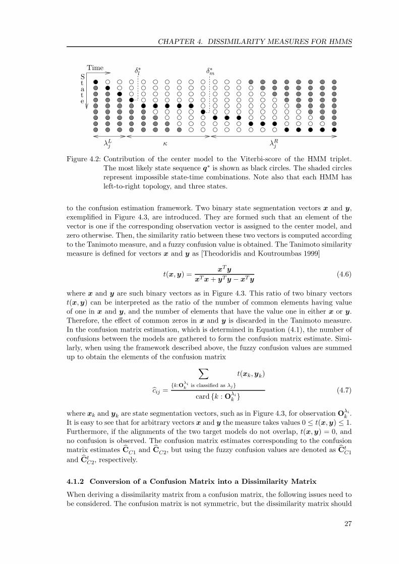
CHAPTER 4. DISSIMILARITY MEASURES FOR HMMS
λLj κ λR
j
δ∗l δ∗mTime
S
at
t
e
Figure 4.2: Contribution of the center model to the Viterbi-score of the HMM triplet.The most likely state sequence q∗ is shown as black circles. The shaded circlesrepresent impossible state-time combinations. Note also that each HMM hasleft-to-right topology, and three states.
to the confusion estimation framework. Two binary state segmentation vectors x and y,exemplified in Figure 4.3, are introduced. They are formed such that an element of thevector is one if the corresponding observation vector is assigned to the center model, andzero otherwise. Then, the similarity ratio between these two vectors is computed accordingto the Tanimoto measure, and a fuzzy confusion value is obtained. The Tanimoto similaritymeasure is defined for vectors x and y as [Theodoridis and Koutroumbas 1999]
t(x,y) =xT y
xT x + yT y − xT y(4.6)
where x and y are such binary vectors as in Figure 4.3. This ratio of two binary vectorst(x,y) can be interpreted as the ratio of the number of common elements having valueof one in x and y, and the number of elements that have the value one in either x or y.Therefore, the effect of common zeros in x and y is discarded in the Tanimoto measure.In the confusion matrix estimation, which is determined in Equation (4.1), the number ofconfusions between the models are gathered to form the confusion matrix estimate. Simi-larly, when using the framework described above, the fuzzy confusion values are summedup to obtain the elements of the confusion matrix
cij =
∑{k:O
λik is classified as λj}
t(xk,yk)
card {k : Oλik } (4.7)
where xk and yk are state segmentation vectors, such as in Figure 4.3, for observation Oλik .
It is easy to see that for arbitrary vectors x and y the measure takes values 0 ≤ t(x,y) ≤ 1.Furthermore, if the alignments of the two target models do not overlap, t(x,y) = 0, andno confusion is observed. The confusion matrix estimates corresponding to the confusionmatrix estimates CC1 and CC2, but using the fuzzy confusion values are denoted as Ct
C1
and CtC2, respectively.
4.1.2 Conversion of a Confusion Matrix into a Dissimilarity Matrix
When deriving a dissimilarity matrix from a confusion matrix, the following issues need tobe considered. The confusion matrix is not symmetric, but the dissimilarity matrix should
27
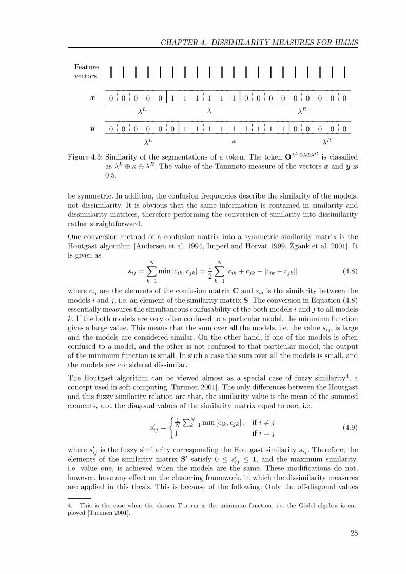
CHAPTER 4. DISSIMILARITY MEASURES FOR HMMS
0000000000 0 0 0 0
00000000000
111111
111111111
x
y
Featurevectors
λL
λL
λR
λRλ
κ
Figure 4.3: Similarity of the segmentations of a token. The token OλL⊕λ⊕λRis classified
as λL ⊕ κ⊕ λR. The value of the Tanimoto measure of the vectors x and y is0.5.
be symmetric. In addition, the confusion frequencies describe the similarity of the models,not dissimilarity. It is obvious that the same information is contained in similarity anddissimilarity matrices, therefore performing the conversion of similarity into dissimilarityrather straightforward.
One conversion method of a confusion matrix into a symmetric similarity matrix is theHoutgast algorithm [Andersen et al. 1994, Imperl and Horvat 1999, Zgank et al. 2001]. Itis given as
sij =N∑
k=1
min [cik, cjk] =12
N∑k=1
[cik + cjk − |cik − cjk|] (4.8)
where cij are the elements of the confusion matrix C and sij is the similarity between themodels i and j, i.e. an element of the similarity matrix S. The conversion in Equation (4.8)essentially measures the simultaneous confusability of the both models i and j to all modelsk. If the both models are very often confused to a particular model, the minimum functiongives a large value. This means that the sum over all the models, i.e. the value sij, is largeand the models are considered similar. On the other hand, if one of the models is oftenconfused to a model, and the other is not confused to that particular model, the outputof the minimum function is small. In such a case the sum over all the models is small, andthe models are considered dissimilar.
The Houtgast algorithm can be viewed almost as a special case of fuzzy similarity4, aconcept used in soft computing [Turunen 2001]. The only differences between the Houtgastand this fuzzy similarity relation are that, the similarity value is the mean of the summedelements, and the diagonal values of the similarity matrix equal to one, i.e.
s′ij =
{1N
∑Nk=1 min [cik, cjk] , if i �= j
1 if i = j(4.9)
where s′ij is the fuzzy similarity corresponding the Houtgast similarity sij . Therefore, theelements of the similarity matrix S′ satisfy 0 ≤ s′ij ≤ 1, and the maximum similarity,i.e. value one, is achieved when the models are the same. These modifications do not,however, have any effect on the clustering framework, in which the dissimilarity measuresare applied in this thesis. This is because of the following: Only the off-diagonal values
4. This is the case when the chosen T-norm is the minimum function, i.e. the Godel algebra is em-ployed [Turunen 2001].
28

CHAPTER 4. DISSIMILARITY MEASURES FOR HMMS
are employed in the clustering procedure. In other words, only the HMMs having differentmodel indices are compared against each other. In addition, the similarity values arecompared only against each other, meaning that the scaling does not have effect on theclustering procedure.
The conversion from a similarity matrix into a dissimilarity matrix can be performed usingbasically any monotonically decreasing function. The choice of such function depends onthe nature of the application in which the dissimilarity matrix is to be used. The clus-tering can be performed using agglomerative clustering algorithm with complete linkagecriterion, explained in Algorithm 3.1. As this procedure uses maximum dissimilarity in thecluster merging criterion, it is obvious that the clustering does not depend on the choise ofthe function used in the similarity-to-dissimilarity conversion. For example, the followingsimple function can be applied for this coversion
dij = 1 − s′ij (4.10)
where dij is the element of the dissimilarity matrix D corresponding the fuzzy similaritymatrix S′.
4.2 Measures Based on Kullback-Leibler Divergence
The dissimilarity measures described in Section 4.1 were based on the classification errorsmade by the recognition system. Alternatively, the dissimilarity of stochastic models canbe measured based on the distributions of the models. A well-known dissimilarity measurebetween two probability distributions is the Kullback-Leibler divergence. It characterizesthe discriminating properties of two probabilistic models λ and κ, and is defined as [Kull-back 1968]
J(λ, κ) = I(λ : κ) + I(κ : λ) (4.11)
where
I(λ : κ) = E
{log
f(Oλ;λ)f(Oλ;κ)
}(4.12)
is the directed divergence from λ to κ. In Equation (4.12), the expectation E is taken withrespect to the random variable Oλ corresponding the distribution of the model λ, and theprobability density functions of the corresponding models are denoted by f(Oλ; ·).The Kullback-Leibler (KL) divergence measure cannot usually be presented for HMMsin a closed form. Therefore, some approximations of this measure have been introduced[Falkhausen et al. 1995, Juang and Rabiner 1985, Kohler 2001]. These approximations arebased on Monte Carlo (MC) methods or simplifying approximations that lead to a closedform solution. In practice, the drawbacks of MC techniques are the extensive computa-tional cost and slow convergence properties. On the other hand, the closed form approx-imations presented are limited to very specific class of HMMs, e.g. HMMs with discreteobservation densities [Falkhausen et al. 1995]. The above mentioned methods are reviewedin Sections 4.2.1–4.2.3. The previously presented closed-form solution is extended to con-tinuous distributions in Section 4.2.3. In addition, a modified approximation is presentedin Section 4.2.3, that is supposed to be more accurate.
29

CHAPTER 4. DISSIMILARITY MEASURES FOR HMMS
4.2.1 Monte-Carlo Techniques
Juang et al. studied the KL-divergence between HMMs using MC simulations. The modelswere assumed ergodic, and the measure was defined as the mean divergence per observationsample [Juang and Rabiner 1985]. The measure was given as
IMC(λ : κ) =1T
logP (Oλ | λ)P (Oλ | κ) (4.13)
where Oλ is an observation sequence generated by model λ. In addition, the length of thesequence is denoted with T , and the likelihoods given the models λ and κ are given asP (Oλ | λ) and P (Oλ | κ), respectively. The method is valid for HMMs with arbitraryobservation probability distributions [Juang and Rabiner 1985].
Some approximations of the measure in Equation (4.13) were proposed and comparedin [Falkhausen et al. 1995]. In that article, the assumed ergodicity property of the originallyleft-to-right models was achieved by substituting the transitions to non-emitting statewith transitions to the first emitting state. The resulting measure, denoted by I∗MC , wasobtained by substituting the likelihoods P (O | ·) in Equation (4.13) with likelihoods ofthe most likely state sequences P ∗(O | ·) = max�∈Q P (O,q | ·)5. Only minor differenceswere observed when comparing the behavior of IMC and I∗MC [Falkhausen et al. 1995].
4.2.2 Monte-Carlo Estimates based on Speech Data
A variant of the measure given in Equation (4.13) was proposed in [Kohler 2001]. Tokensextracted from speech corpus were used in the evaluation of the measure instead of a gen-erated random sequence. Furthermore, the models were not ergodic as in Equation (4.13),but left-to-right phone models. Estimate of the divergence was defined as a sample meanof the log-likelihood differences over the tokens
I(λ : κ) =1N
N∑i=1
1Ti
logP (Oλ
i | λ)P (Oλ
i | κ) (4.14)
where Oλi is the i:th token of length Ti corresponding the model λ. Experimental results
showed that the obtained estimates of the divergence measure were applicable in phonememodel clustering [Kohler 2001]. As Falkhausen et. al. proposed, the likelihood of the mostlikely state sequence P ∗(O | ·) can be used instead of P (O | ·) in Equation (4.14), whichresults in the estimate
IS(λ : κ) =1N
N∑i=1
1Ti
logP ∗(Oλ
i | λ)P ∗(Oλ
i | κ) =1N
N∑i=1
LLRS(Oλi | λ, κ) (4.15)
where the function LLRS(O | λ, κ) denotes the logarithmic likelihood ratio of O given λand κ, respectively. The logarithmic likelihoods in Equation (4.15) are in fact the verysame values that were used as likelihood scores in evaluation of the confusion matrix CS.Therefore, the function can be written as
LLRS(Oλi | λ, κ) =
1Ti
[SCS(Oλ
i | λ) − SCS(Oλi | κ)
](4.16)
5. This can be obtained using the Viterbi-decoding described in Algorithm 2.3.
30
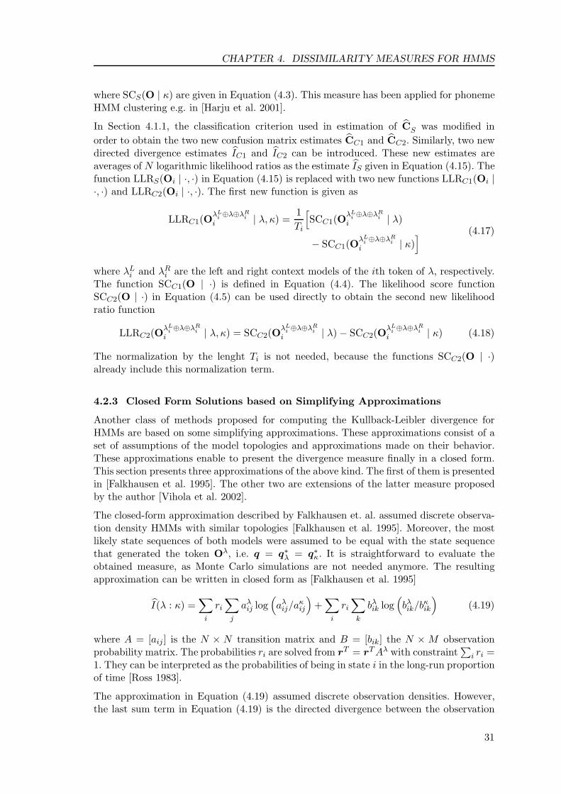
CHAPTER 4. DISSIMILARITY MEASURES FOR HMMS
where SCS(O | κ) are given in Equation (4.3). This measure has been applied for phonemeHMM clustering e.g. in [Harju et al. 2001].
In Section 4.1.1, the classification criterion used in estimation of CS was modified inorder to obtain the two new confusion matrix estimates CC1 and CC2. Similarly, two newdirected divergence estimates IC1 and IC2 can be introduced. These new estimates areaverages of N logarithmic likelihood ratios as the estimate IS given in Equation (4.15). Thefunction LLRS(Oi | ·, ·) in Equation (4.15) is replaced with two new functions LLRC1(Oi |·, ·) and LLRC2(Oi | ·, ·). The first new function is given as
LLRC1(OλL
i ⊕λ⊕λRi
i | λ, κ) =1Ti
[SCC1(O
λLi ⊕λ⊕λR
ii | λ)
− SCC1(OλL
i ⊕λ⊕λRi
i | κ)] (4.17)
where λLi and λR
i are the left and right context models of the ith token of λ, respectively.The function SCC1(O | ·) is defined in Equation (4.4). The likelihood score functionSCC2(O | ·) in Equation (4.5) can be used directly to obtain the second new likelihoodratio function
LLRC2(OλL
i ⊕λ⊕λRi
i | λ, κ) = SCC2(OλL
i ⊕λ⊕λRi
i | λ) − SCC2(OλL
i ⊕λ⊕λRi
i | κ) (4.18)
The normalization by the lenght Ti is not needed, because the functions SCC2(O | ·)already include this normalization term.
4.2.3 Closed Form Solutions based on Simplifying Approximations
Another class of methods proposed for computing the Kullback-Leibler divergence forHMMs are based on some simplifying approximations. These approximations consist of aset of assumptions of the model topologies and approximations made on their behavior.These approximations enable to present the divergence measure finally in a closed form.This section presents three approximations of the above kind. The first of them is presentedin [Falkhausen et al. 1995]. The other two are extensions of the latter measure proposedby the author [Vihola et al. 2002].
The closed-form approximation described by Falkhausen et. al. assumed discrete observa-tion density HMMs with similar topologies [Falkhausen et al. 1995]. Moreover, the mostlikely state sequences of both models were assumed to be equal with the state sequencethat generated the token Oλ, i.e. q = q∗
λ = q∗κ. It is straightforward to evaluate the
obtained measure, as Monte Carlo simulations are not needed anymore. The resultingapproximation can be written in closed form as [Falkhausen et al. 1995]
I(λ : κ) =∑
i
ri∑
j
aλij log
(aλ
ij/aκij
)+
∑i
ri∑
k
bλik log(bλik/b
κik
)(4.19)
where A = [aij ] is the N × N transition matrix and B = [bik] the N ×M observationprobability matrix. The probabilities ri are solved from rT = rTAλ with constraint
∑i ri =
1. They can be interpreted as the probabilities of being in state i in the long-run proportionof time [Ross 1983].
The approximation in Equation (4.19) assumed discrete observation densities. However,the last sum term in Equation (4.19) is the directed divergence between the observation
31

CHAPTER 4. DISSIMILARITY MEASURES FOR HMMS
��������
����
��������
��
����
��
����
λ
λκ
κ r1 r2 r3
w1 w2 w3 w4
state
a b
(1,1) (1,2) (2,2) (3,3)1
1
2
2
3
3
Figure 4.4: State alignment in divergence approximation. The possible state alignments ofthe models λ and κ are shown as dotted lines in (a). The solid line correspondsthe alignment of the models shown in (b). The symbols ri and wi are the onesused in Equation 4.22.
distributions of state i of the models λ and κ. Thus, we can rewrite the Equation (4.19)in the form
IA1(λ : κ) =∑
i
ri∑
j
aλij log
(aλ
ij/aκij
)+
∑i
riI(bλi : bκi ) (4.20)
where bλi and bκi are the observation probability distributions of the models λ and κ instate i, respectively. Now, the only terms that are dependent of the observation probabil-ity distributions are the directed divergences between the corresponding distributions ofthe states, I(bλi : bκi ). The Equation (4.20) generalizes the Equation (4.19) for arbitraryobservation densities. The other simplifying assumptions made in deriving the approxima-tion in Equation (4.19) still remain. In the case of Gaussian observation distributions, thecross-state directed divergences can be expressed in a closed form as [Kullback 1968]
I(b1 : b2) =12
[log
|Σ2||Σ1| + tr
(Σ1(Σ−1
2 −Σ−11 )
)+ tr
(Σ−1
2 (µ1 − µ2)(µ1 − µ2)T) ] (4.21)
where Σ and µ denote the covariance matrices and the mean vectors of the distributions,respectively.
The assumption made in deriving the approximation in Equation (4.20) is that the mostlikely state sequences of both of the models are equal to the state sequence of the generatingmodel, i.e. q = q∗
λ = q∗κ. This assumption can be considered realistic with the model λ.
However, there is no reason to assume that the model κ would follow the same sequence.Let us draw one sample from the observation distribution of i:th state of the model λ.It is easy to agree that in most of the cases the likelihood of the generating distributionis greater than likelihoods given by other distributions. This justifies why the most likelystate sequence of model λ should correspond the generating sequence, q∗
λ = q in average.Considering the state sequence q∗
κ of the model κ, the best likelihood for this model ismost likely given by the state-dependent density closest to the corresponding density ofλ. This gives us a reason to find such a state alignment between the models λ and κ thatthe states with best matching distributions coincide.
Assume now that the both HMMs have left-to-right topologies, such as the model shownin Figure 2.3. The transitions in these models are either self-transitions or transitions
32
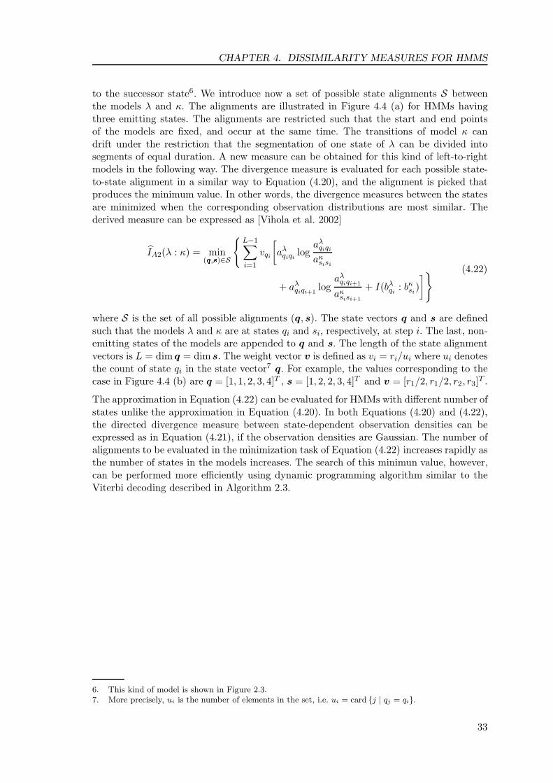
CHAPTER 4. DISSIMILARITY MEASURES FOR HMMS
to the successor state6. We introduce now a set of possible state alignments S betweenthe models λ and κ. The alignments are illustrated in Figure 4.4 (a) for HMMs havingthree emitting states. The alignments are restricted such that the start and end pointsof the models are fixed, and occur at the same time. The transitions of model κ candrift under the restriction that the segmentation of one state of λ can be divided intosegments of equal duration. A new measure can be obtained for this kind of left-to-rightmodels in the following way. The divergence measure is evaluated for each possible state-to-state alignment in a similar way to Equation (4.20), and the alignment is picked thatproduces the minimum value. In other words, the divergence measures between the statesare minimized when the corresponding observation distributions are most similar. Thederived measure can be expressed as [Vihola et al. 2002]
IA2(λ : κ) = min(�,�)∈S
{L−1∑i=1
vqi
[aλ
qiqilog
aλqiqi
aκsisi
+ aλqiqi+1
logaλ
qiqi+1
aκsisi+1
+ I(bλqi: bκsi
)]} (4.22)
where S is the set of all possible alignments (q, s). The state vectors q and s are definedsuch that the models λ and κ are at states qi and si, respectively, at step i. The last, non-emitting states of the models are appended to q and s. The length of the state alignmentvectors is L = dim q = dims. The weight vector v is defined as vi = ri/ui where ui denotesthe count of state qi in the state vector7 q. For example, the values corresponding to thecase in Figure 4.4 (b) are q = [1, 1, 2, 3, 4]T , s = [1, 2, 2, 3, 4]T and v = [r1/2, r1/2, r2, r3]T .
The approximation in Equation (4.22) can be evaluated for HMMs with different number ofstates unlike the approximation in Equation (4.20). In both Equations (4.20) and (4.22),the directed divergence measure between state-dependent observation densities can beexpressed as in Equation (4.21), if the observation densities are Gaussian. The number ofalignments to be evaluated in the minimization task of Equation (4.22) increases rapidly asthe number of states in the models increases. The search of this minimun value, however,can be performed more efficiently using dynamic programming algorithm similar to theViterbi decoding described in Algorithm 2.3.
6. This kind of model is shown in Figure 2.3.7. More precisely, ui is the number of elements in the set, i.e. ui = card {j | qj = qi}.
33

Chapter 5
Experimental Setup and Results
The dissimilarity measures covered in Chapter 4 were experimented in the task of phonememodel clustering. The clustering was used for defining a set of multilingual phone models fora multilingual speech recognition system. The word recognition accuracy of the resultingspeech recognition systems was evaluated in speaker independent isolated word recognitiontask. The experiments were evaluated with The Hidden Markov Model Toolkit (HTK),which provided efficient implementations of algorithms used in both training and testingof the speech recognition systems [Young et al. 2000]. The estimation of the dissimilaritymeasures and the clustering framework were implemented with Matlab 5.3 [MAT].
The content of this chapter is briefly following. Section 5.1 describes the speech corpora andthe front-end unit employed for the experiments. After that, the configuration and trainingof the language dependent baseline ASR systems is explained in Section 5.2. In addition,the test setup and the word recognition accuracies of the baseline systems are describedin detail. Section 5.3 covers the derivation and testing of the different multilingual ASRsystems. Finally, in Section 5.4, a summary and a comparison of the recognition results ofthe ML systems are given.
5.1 Speech Corpora and Front-End
All the experiments were performed using the SpeechDat(II) speech corpora of seven lan-guages: English, Finnish, French, German, Italian, Spanish and Swedish [Winski 1997].The speech utterances in the SpeechDat(II) corpora have been recorded over a fixed tele-phone network. The sample files are in raw 8bit A-law data format, with 8kHz samplingfrequency. The speech utterances in the corpora are annotated in word level, but withoutany word boundary information. However, the annotation contains additional informationof e.g. strong background noise, truncation of a sentence or speaker-specific noise occuredduring the recording session. In some of the languages, the utterances with speaker-specificnoise were included in the experiments, due to shortage of data. The last column in Ta-bles 5.1–5.3 indicate whether such utterances were included in the data sets. The wordpronunciation lexicons in the SpeechDat(II) corpora are written with the SAMPA phoneticsymbols [SAM]. These phonetic symbols are used in this chapter to denote the phonemes.
The speech material was parametrized using a Mel-frequency cepstral coefficient (MFCC)front-end described in Section 2.3. The frame interval and window length used in the front-end were 10ms and 25ms, respectively. For each frame, the front-end produced a featurevector consisting of 13 Mel-cepstral coefficients of which the zeroth, C0, was replaced withframe energy E. The first and second time derivatives of the elements were appended
34
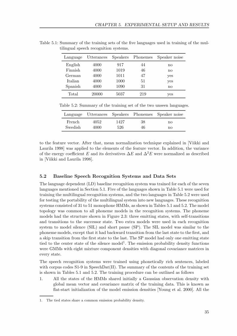
CHAPTER 5. EXPERIMENTAL SETUP AND RESULTS
Table 5.1: Summary of the training sets of the five languages used in training of the mul-tilingual speech recognition systems.
Language Utterances Speakers Phonemes Speaker noise
English 4000 917 44 noFinnish 4000 1019 46 noGerman 4000 1011 47 yesItalian 4000 1000 51 yesSpanish 4000 1090 31 no
Total 20000 5037 219 yes
Table 5.2: Summary of the training set of the two unseen languages.
Language Utterances Speakers Phonemes Speaker noise
French 4052 1427 38 noSwedish 4000 526 46 no
to the feature vector. After that, mean normalization technique explained in [Viikki andLaurila 1998] was applied to the elements of the feature vector. In addition, the varianceof the energy coefficient E and its derivatives ∆E and ∆2E were normalized as describedin [Viikki and Laurila 1998].
5.2 Baseline Speech Recognition Systems and Data Sets
The language dependent (LD) baseline recognition system was trained for each of the sevenlanguages mentioned in Section 5.1. Five of the languages shown in Table 5.1 were used fortraining the multilingual recognition systems, and the two languages in Table 5.2 were usedfor testing the portability of the multilingual system into new languages. These recognitionsystems consisted of 31 to 51 monophone HMMs, as shown in Tables 5.1 and 5.2. The modeltopology was common to all phoneme models in the recognition systems. The phonememodels had the structure shown in Figure 2.3: three emitting states, with self-transitionsand transitions to the successor state. Two extra models were used in each recognitionsystem to model silence (SIL) and short pause (SP). The SIL model was similar to thephoneme models, except that it had backward transition from the last state to the first, anda skip transition from the first state to the last. The SP model had only one emitting statetied to the center state of the silence model1. The emission probability density functionswere GMMs with eight mixture component densities with diagonal covariance matrices inevery state.
The speech recognition systems were trained using phonetically rich sentences, labeledwith corpus codes S1-9 in SpeechDat(II). The summary of the contents of the training setis shown in Tables 5.1 and 5.2. The training procedure can be outlined as follows1. All the states of the HMMs shared initially a Gaussian observation density with
global mean vector and covariance matrix of the training data. This is known asflat-start initialization of the model emission densities [Young et al. 2000]. All the
1. The tied states share a common emission probability density.
35

CHAPTER 5. EXPERIMENTAL SETUP AND RESULTS
HMMs, including the SIL model had equivalent initial topology. The SP model wasomitted at this stage of the training. The initial state distribution and the transitionprobabilities of the HMMs were set to π1 = 1, a11 = a22 = 0.6, a23 = a34 = 0.4,a33 = 0.7 and a34 = 0.3. Other elements of π and A were constrained zero.
2. The parameters of HMMs were re-estimated using the embedded Baum-Welch(BW) re-estimation procedure explained in Section 2.4.3. Three iterations of thealgorithm were performed over the full training data set.
3. Two extra transitions, the skip and the backward transition, were included tothe SIL model, a13 = a31 = 0.2. The other transition probabilities of the modelwere modified such that
∑j aij = 1, for all i. The SP model was included at this
time. The model consisted of one emitting state, namely the state two of SIL.The observation density parameters of the SP state and the second state of SILwere tied. A so called tee-transition, i.e. a transition over the emitting state of themodel π2 = 0.3, was included to the SP model. Finally, two iterations of BW wereperformed for the HMMs in the recognition system.
4. A realignment of the training utterances was performed next. This means that thetraining utterances were recognized with current HMMs, and the best matchingpronunciations of the words in the utterance were chosen, when there were duplicatepronunciations in the lexicon. After the realignment of the training utterances, twoiterations of the BW re-estimation were performed to the HMMs.
5. The Gaussian emission densities of the HMMs were replaced gradually with mixture-Gaussian densities. The number of mixture components was incremented by one ata time2, and after each incrementation of the components, an iteration of BW re-estimation was performed over the full training data set. This mixture incrementingwas repeated until the final number of mixtures, eight, was achieved. Finally, eightmore iterations of the BW re-estimation were performed.
The final LD recognition systems were tested in isolated word recognition task. The sum-mary of the test sets is shown in Table 5.3. The number of vocabulary items was around200 in each language. The test set of a language covered 3000–4000 samples includingapplication words (A1-3), isolated digits (I1) and forename-surname combinations3 (O7).The average word recognition rates of the baseline LD recognition systems are shown inTable 5.4. The differences between languages as well as different vocabulary items aresubstantial. The shorter items, i.e. application words and digits were recognized poorlycompared to the longer forename-surname combinations, especially in English and Germanlanguages. This reflects into the inferior average word recognition rate (WRR) of theselanguages.
5.3 Multilingual Recognition Systems
The multilingual (ML) recognition systems were trained using the training data for the fivesource languages shown in Table 5.1. The training procedure as well as the model config-uration were identical to the LD recognizers described in Section 5.2. The only differencewas that the label files and the lexicon were changed to correspond to the phone cluster
2. This mixture incrementation was performed such that the mixture component with the greatest weightwas split, meaning that the mixture component was copied, the weights were divided by two, and the meanswere perturbed by plus or minus 0.2 times the standard deviations [Young et al. 2000].3. The forename-surname combinations were recognized as one unit, i.e. the arbitrary combinations ofthe forenames and surnames were not allowed.
36

CHAPTER 5. EXPERIMENTAL SETUP AND RESULTS
Table 5.3: Summary of the test sets
Number of utterances Vocab. Speaker
Language A1 A2 A3 I1 O7 Total Speakers items noise
English 800 800 800 800 800 4000 1228 194 noFinnish 800 800 800 800 800 4000 1024 194 noGerman 800 800 800 800 800 4000 1582 196 yesItalian 800 800 800 800 800 4000 1349 201 yesSpanish 800 800 800 800 800 4000 1513 193 no
French 600 600 600 600 600 3000 1158 190 yesSwedish 800 805 807 803 781 3996 1435 190 no
Total 5400 5405 5407 5403 5381 26996 9289 - yes
Table 5.4: Average word recognition rates of the seven LD baseline recognition systems.
Language A1 A2 A3 I1 O7 Avg.
English 78.75 78.25 78.62 64.38 91.93 78.40Finnish 93.91 95.15 94.05 96.50 98.38 95.35German 82.75 83.50 80.75 75.62 95.16 83.32Italian 89.50 94.88 87.25 92.38 96.52 92.07Spanish 98.38 97.23 95.12 93.00 96.44 95.78
French 88.05 87.72 88.28 62.67 92.12 83.57Swedish 90.06 87.27 89.52 71.64 95.40 85.29
symbols of each ML recognition system. The determination of these phone clusters wasbased on either expert knowledge or agglomerative clustering. This clustering was basedon the dissimilarity measures between the phoneme HMMs of the baseline LD recogni-tion systems. These dissimilarity measures and the agglomerative clustering algorithm aredescribed in Chapter 4 and Algorithm 3.1, respectively. The obtained ML systems weretested similarly as the LD systems described in Section 5.2. During the recognition, onlythe vocabulary of the target language was set active. The Sections 5.3.1–5.3.3 review thederivation and the experiments performed with the ML recognition systems.
5.3.1 Knowledge-based Multilingual Recognition Systems
The multilingual recognition system SAMPA was based on the method IPA-MAP de-scribed in Section 3.3.1. The phonemes of different languages were clustered according totheir phonetic SAMPA symbol. The derived SAMPA system had a total of 105 multilin-gual phone models corresponding to all the unique SAMPA symbols present within thedatabases of the five source languages.
The second knowledge-based recognition system, referred to as SR, was obtained withstraightforward simplifications of the phone cluster definitions of SAMPA. The recognitionsystem had no explicit models for long vowels and double consonants. Such phones werereplaced with two single ones, e.g. /e:/ and /ee/ → /e/⊕/e/. In addition, the geminateaffricates in Italian language were replaced with the preceding plosive and the following
37

CHAPTER 5. EXPERIMENTAL SETUP AND RESULTS
Table 5.5: Tying of the rare phoneme models in Finnish, Italian and German.
Finnish Italian German
/gg/ → Italian /gg/ /@/ → English /@/ /o˜/ → Italian /o//bb/ → Italian /bb/ /dz/ → Italian /dZ/ /Z/ → English /Z//dd/ → Italian /dd/ /J/ → Spanish /J/ /a˜/ → Italian /a//ff/ → Italian /ff/ /L/ → Spanish /L/ /dZ/ → English /dZ//hh/ → Finnish /h/ /S/ → German /S/
affricate, e.g. /ddz/ → /d/⊕/dz/. When these simplifications were employed, the totalnumber of phone models was reduced to 64 from 105 of the SAMPA system.
5.3.2 Multilingual Recognition Systems based on Dissimilarity Measures
All the multilingual systems based on dissimilarity measures had a total of 64 phonemodels. The phone model definitions in such ML recognition systems were created asfollows. The symmetric dissimilarity matrices D were created according to the particulardissimilarity estimate. Each dissimilarity matrix was applied in the clustering framework,and the derived phone cluster configuration was used for training a ML recognition systemhaving 64 phone models. The agglomerative clustering used in the phone cluster definitionis described in Algorithm 3.1.
The dissimilarity measure estimates were obtained for both Gaussian and eight-mixtureGMM observation density HMMs. The phoneme models of the fully trained LD recognitionsystems were the HMMs with eight-mixture GMM observation densities. The Gaussianobservation density HMMs were obtained from the training procedure of the LD recogni-tion systems, just before the first mixture split. The estimates of the dissimilarity measureswere obtained using up to 1000 tokens for each LD phoneme model. These tokens wereextracted from training speech material according to phoneme level segmentation of theutterances. The segmentation of the utterances was obtained using the fully trained LDrecognition systems explained in Section 5.2. The phoneme models that did not have suf-ficient number of tokens for estimating the dissimilarity measures (under 50 tokens) werenot included in the clustering framework. Instead, they were assigned manually to thecluster having the most similar LD phoneme. The tying of these rare phoneme models isshown in Table 5.5. In addition, the clustering was constrained such that phoneme modelsof the same language were not allowed to locate in a same cluster, excluding the man-ually tied rare phonemes. This clustering procedure was applied identically with all thedissimilarity measures.
The experiments were carried out with the dissimilarity measures evaluated from theconfusion matrix estimates CS, CC1, CC2, Ct
C1 and CtC2, and from the KL divergence
estimates. These KL divergence estimates JX were obtained according to Equation (4.11)from the corresponding directed divergence measures IX . The three directed divergenceestimates IS , IC1 and IC2, as well as the two closed-form approximations IA1 and IA2,were employed in the experiments. The latter two approximations were evaluated only formodels with Gaussian observation densities, as these approximations cannot be presentedin a closed form with mixture observation density HMMs. The measures are referred hereaccording the terminology in Chapter 4. Specifically, the definitions of these estimatesare given in Equations (4.2)–(4.22). The number of mixture density components in the
38
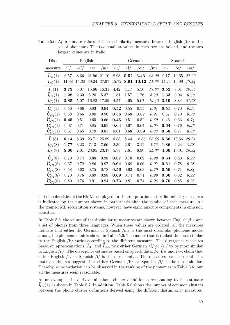
CHAPTER 5. EXPERIMENTAL SETUP AND RESULTS
Table 5.6: Approximate values of the dissimilarity measures between English /i:/ and aset of phonemes. The two smallest values in each row are bolded, and the twolargest values are in italic.
Diss. English German Spanish
measure /I/ /eI/ /e/ /m/ /i:/ /I/ /e:/ /m/ /i/ /e/ /m/
IA1(1) 6.57 8.66 21.96 21.10 8.98 5.52 5.43 23.00 9.17 10.65 27.29IA2(1) 11.38 15.38 39.24 37.97 15.72 8.91 10.12 41.68 14.24 19.99 47.34
IS(1) 3.73 5.07 15.86 16.31 4.42 4.17 5.50 17.87 3.52 8.01 20.05IC1(1) 1.28 2.30 5.20 5.37 1.81 1.57 1.76 5.70 1.33 3.04 6.22IC2(1) 3.85 5.07 16.83 17.59 4.57 4.65 5.07 19.42 3.19 8.84 21.68
CS(1) 0.56 0.66 0.83 0.94 0.52 0.55 0.55 0.94 0.51 0.70 0.95CC1(1) 0.58 0.66 0.80 0.90 0.56 0.58 0.57 0.91 0.57 0.70 0.93CC2(1) 0.45 0.51 0.65 0.66 0.45 0.51 0.52 0.69 0.46 0.63 0.74Ct
C1(1) 0.67 0.71 0.85 0.95 0.64 0.67 0.64 0.95 0.64 0.76 0.96Ct
C2(1) 0.67 0.65 0.79 0.81 0.61 0.68 0.59 0.83 0.58 0.71 0.83
IS(8) 6.14 8.39 23.71 25.89 6.58 8.44 10.55 25.65 5.36 13.56 29.51IC1(8) 1.77 3.23 7.13 7.66 2.39 2.61 3.12 7.73 1.86 4.24 8.68IC2(8) 5.66 7.01 23.95 23.47 5.73 7.61 8.90 24.07 4.66 13.01 26.94
CS(8) 0.70 0.74 0.88 0.98 0.67 0.70 0.69 0.98 0.64 0.80 0.99CC1(8) 0.67 0.72 0.86 0.97 0.64 0.68 0.66 0.97 0.61 0.78 0.98CC2(8) 0.58 0.63 0.75 0.78 0.56 0.62 0.63 0.79 0.56 0.71 0.84Ct
C1(8) 0.73 0.76 0.89 0.98 0.69 0.74 0.71 0.99 0.66 0.82 0.99Ct
C2(8) 0.80 0.76 0.91 0.94 0.73 0.81 0.74 0.96 0.70 0.85 0.96
emission densities of the HMMs employed for the computation of the dissimilarity measuresis indicated by the number shown in parenthesis after the symbol of each measure. Allthe trained ML recognition systems, however, have eight mixture components in emissiondensities.
In Table 5.6, the values of the dissimilarity measures are shown between English /i:/ anda set of phones from three languages. When these values are ordered, all the measuresindicate that either the German or Spanish /m/ is the most dissimilar phoneme modelamong the phoneme models shown in Table 5.6. The model that is ranked the most similarto the English /i:/ varies according to the different measures. The divergence measuresbased on approximations, IA1 and IA2, pick either German /I/ or /e:/ to be most similarto English /i:/. The divergence estimates based on speech data, IS , IC1 and IC2, claim thateither English /I/ or Spanish /i/ is the most similar. The measures based on confusionmatrix estimates suggest that either German /i:/ or Spanish /i/ is the most similar.Thereby, some variation can be observed in the ranking of the phonemes in Table 5.6, butall the measures seem reasonable.
As an example, the derived full phone cluster definition corresponding to the estimateIC2(1), is shown in Table 5.7. In addition, Table 5.8 shows the number of common clustersbetween the phone cluster definitions derived using the different dissimilarity measures.
39

CHAPTER 5. EXPERIMENTAL SETUP AND RESULTS
Table 5.7: Phone cluster definitions derived from the dissimilarity estimate IC2(1). Themanually assigned rare phonemes are shown in parenthesis. This table continueson Page 41.
Phone cluster English Finnish German Italian Spanish
1 U Y2 d g3 oo aU O4 U@5 h h, (hh) h6 dZ, (dz) jj7 I i I8 LL, (L) L9 u: yy 2:10 JJ, (J) J11 N N N N12 (dd) dd13 V 614 nn nn D15 aI aI16 ll ll17 @U A a18 b b19 j ddZ20 3: 22
Most of these definitions are very different compared against each other. In most of thecases, only less than half of the phone clusters in the definitions are common.
5.3.3 Unseen Languages
There were two unseen languages, French and Swedish, included in the tests. They areunseen, since no data was used from these languages in the training of the ML recog-nition systems. The tying of the phonemes of these languages was based on phoneticknowledge [Raimo and Savela 2001]. Each phoneme was tied explicitly to one languagedependent phoneme model of the five source languages. This tying is shown in Table 5.9.Based on this information, each phoneme of the unseen languages was mapped to a MLphone model accordingly. The tying shown in Table 5.9 was same within all the evaluatedML recognition systems.
The cross-language transfer (CLT) was experimented also for the two unseen languages.The LD recognition systems of the five source languages were employed for this transfer.The systems were obtained for French and Swedish by gathering the necessary phonememodels from the source LD recognizers to form a new CLT recognition system. The gath-ering of the models was performed according to the tying in Table 5.9, thus similarly asin the case of ML recognition systems. The silence and short pause models of the CLTsystems were obtained from the Spanish LD recognition system.
40

CHAPTER 5. EXPERIMENTAL SETUP AND RESULTS
Table 5.7: Continued from Page 40.
Phone cluster English Finnish German Italian Spanish
21 OI OY22 NN vv g23 ts ts24 e@ 225 tS tS tS26 @ v @ v, (@) B27 S C SS28 e e E e29 l u: u G30 T f, (ff) pf ff31 D y y: ddz32 Q o O, (o˜) o o33 Z s S, (Z) (S) s34 u U u35 r rr 9 rr rr36 A: AA a:37 b b, (bb) b bb38 I@ ee E: E39 d (gg) d gg40 eI e: e41 f f f f42 g g g d d43 k k k k k44 l l l l45 m m m m m46 n n n n n47 i: ii i: i i48 p p p p p49 r r r r50 s s s51 t t t t t52 v v tts T53 kk x kk x54 z z z z55 O: uu o:56 dZ (dZ) ttS tS57 j j j j58 w w w59 aU {{60 { { (a˜) a a61 ss ss62 pp pp63 tt tt64 mm mm
41

CHAPTER 5. EXPERIMENTAL SETUP AND RESULTS
Table 5.8: The number of common phone clusters in the phone cluster definitions obtainedusing the dissimilarity measures. The phone cluster definitions that have at least32 common clusters are bolded. This number is half of the total number of thephone clusters in each ML system.
I A2(1
)
I S(1
)
I C1(1
)
I C2(1
)
CS(1
)
CC
1(1
)
CC
2(1
)
Ct C
1(1
)
Ct C
2(1
)
I S(8
)
I C1(8
)
I C2(8
)
CS(8
)
CC
1(8
)
CC
2(8
)
Ct C
1(8
)
Ct C
2(8
)
IA1(1) 23 12 12 11 8 9 9 10 7 11 9 9 8 8 8 7 6IA2(1) – 17 20 15 14 15 13 14 13 12 15 13 12 11 13 10 9
IS(1) – – 22 26 21 24 20 24 18 22 14 20 22 19 17 19 16IC1(1) – – – 28 25 26 21 21 16 21 22 26 20 18 21 17 15IC2(1) – – – – 23 24 19 21 20 26 19 26 22 20 19 20 20
CS(1) – – – – – 35 22 29 22 23 23 29 29 29 24 26 20CC1(1) – – – – – – 27 38 23 32 28 38 29 30 26 30 27CC2(1) – – – – – – – 21 20 20 21 24 23 25 24 22 21Ct
C1(1) – – – – – – – – 23 30 21 31 30 28 24 28 19Ct
C2(1) – – – – – – – – – 19 19 20 26 23 19 23 22
IS(8) – – – – – – – – – – 25 36 30 28 20 30 26IC1(8) – – – – – – – – – – – 34 31 29 26 29 19IC2(8) – – – – – – – – – – – – 34 31 28 32 25
CS(8) – – – – – – – – – – – – – 45 24 46 24CC1(8) – – – – – – – – – – – – – – 26 53 29CC2(8) – – – – – – – – – – – – – – – 24 25Ct
C1(8) – – – – – – – – – – – – – – – – 28
5.4 Comparison of Recognition Results
The average word recognition rates of the LD and ML speech recognition systems areshown for the test sets in Tables 5.10 and 5.11. The two highest average WRRs of theML systems are bolded, and the two lowest WRRs are shown in italic. In Tables 5.10and 5.11, the ML recognition systems SAMPA and SR are based on expert knowledge,while the other ML recognition systems are based on dissimilarity measures. Table 5.10shows that the degradation in WRR of the test set was moderate within the five sourcelanguages, when comparing the LD recognition systems and the ML recognition systemSAMPA having 105 phone models. The further reduction of the WRR was small, when thenumber of ML phone models was dropped into 64 in the SR system. All the ML recognitionsystems based on computational model tying and employing the data-driven dissimilaritymeasures can be considered comparable to the knowledge based SR system having 64phone models. The systems based on approximations IA1 and IA2 had comparable WRRsto the other ML systems. The WRRs of all these ML recognition systems did not differsignificantly. However, these results show that a ML speech recognition system can bebuilt, in this case, using only 30% of the number of parameters that are used in the LDrecognition systems.
The test set WRRs of the unseen languages are shown in Table 5.11. The WRRs of the
42

CHAPTER 5. EXPERIMENTAL SETUP AND RESULTS
Table 5.9: Mapping of the phonemes of the two unseen languages to the phones included inML recognition systems. In Swedish, the new retroflex consonant phonemes weresplit into separate phones, e.g. /rn/ → /r/⊕/n/, and then mapped accordingly.Similarly, the unseen nasal vowels of French were split into separate vowel andvelar nasal, e.g. /9/ → /9/⊕/N/.
Mapping of the French phonemes
/A/ → English /A:/ /e/ → Italian /e/ /p/ → Italian /p//E/ → Italian /E/ /f/ → Italian /f/ /2/ → German /2://e˜/ → German /E/ /9˜/ → German /9/ /s/ → Italian /s//H/ → Finnish /y/ /g/ → Italian /g/ /t/ → Italian /t//J/ → Italian /J/ /h/ → English /h/ /u/ → Italian /u//N/ → German /N/ /i/ → Italian /i/ /v/ → Italian /v//O/ → Italian /O/ /j/ → Italian /j/ /9/ → German /9//R/ → German /r/ /k/ → Italian /k/ /w/ → Italian /w//S/ → Italian /S/ /l/ → Italian /l/ /o˜/ → German /o˜//Z/ → English /Z/ /m/ → Italian /m/ /y/ → German /y://a/ → Italian /a/ /n/ → Italian /n/ /z/ → German /z//b/ → Italian /b/ /o/ → Italian /o//d/ → Italian /d/ /a˜/ → German /a˜/
Mapping of the Swedish phonemes
/C/ → German /C/ /b/ → English /b/ /n/ → German /n//E/ → German /E/ /E:/ → German /E:/ /i:/ → German /i://u:/ → German /u:/ /d/ → English /d/ /2/ → Finnish /2//I/ → German /I/ /e:/ → German /e:/ /p/ → German /p//9:/ → German /9/ /e/ → Finnish /e/ /r/ → Finnish /r//N/ → German /N/ /f/ → German /f/ /s/ → German /s//O/ → German /O/ /g/ → English /g/ /t/ → German /t//y:/ → German /y:/ /h/ → German /h/ /{/ → Finnish /{//S/ → German /S/ /{:/ → Finnish /{{/ /v/ → English /v//U/ → German /U/ /j/ → German /j/ /9/ → German /9//Y/ → German /Y/ /k/ → German /k/ /o:/ → German /o://A:/ → English /A:/ /l/ → German /l/ /u0/ → English /U//2:/ → German /2:/ /m/ → German /m//a/ → Italian /a/ /}:/ → English /u:/
ML systems were significantly lower compared to the corresponding LD systems, especiallyfor French. The variation on the average WRR is much greater in the unseen languagescompared to the source languages of the ML recognition systems. The systems that werebased on cross-language transfer (CLT) achieved WRRs that are comparable to the MLsystems. Despite the fact that the WRRs of the ML systems was low compared to thecorresponding results of the baseline LD recognition systems of the unseen languages, thiscan be considered as a fair starting point for language or speaker adaptation.
All the ML recognition systems having 64 phone models had comparable WRRs. Thephone cluster definitions of these systems were, however, fundamentally different as shownin Table 5.8. Small differences in values of the dissimilarity measures may cause big dif-
43

CHAPTER 5. EXPERIMENTAL SETUP AND RESULTS
ference in the cluster definitions, due to the nature of the employed clustering algorithm.Furthermore, the dissimilarity measure approximations IA1 and IA2 showed to be applica-ble to the task of multilingual phoneme model clustering. They have, however, significantlylower computational cost compared to the data-driven dissimilarity measures.
44

CHAPTER 5. EXPERIMENTAL SETUP AND RESULTS
Table 5.10: Average test set WRRs of the source languages of the ML recognition systems.
Recognition system English Finnish German Italian Spanish Avg.
LD 78.40 95.35 83.32 92.07 95.78 88.98
SAMPA 63.38 92.30 79.60 93.18 94.55 84.60SR 59.67 91.07 79.07 92.68 93.22 83.14
IA1(1) 65.75 89.40 78.10 89.10 91.28 82.73IA2(1) 64.43 90.05 78.60 91.75 91.45 83.26
IS(1) 63.00 90.97 80.12 92.00 93.00 83.82IC1(1) 65.40 90.65 78.80 92.40 91.70 83.79IC2(1) 65.53 90.95 78.88 93.00 93.62 84.40
CS(1) 63.12 90.88 78.78 92.32 92.88 83.60CC1(1) 65.55 90.07 78.95 92.20 93.47 84.05CC2(1) 63.90 88.10 77.70 91.15 92.78 82.73Ct
C1(1) 65.80 89.68 79.28 91.35 93.55 83.93Ct
C2(1) 64.40 90.32 79.32 91.62 92.72 83.68
IS(8) 64.53 90.55 76.85 92.10 93.30 83.47IC1(8) 67.78 91.15 77.64 90.60 92.20 83.87IC2(8) 63.47 89.20 77.38 92.70 93.43 83.24
CS(8) 64.35 89.75 78.20 92.05 94.38 83.75CC1(8) 66.05 88.97 77.72 92.10 92.95 83.56CC2(8) 63.03 89.32 77.45 89.75 91.57 82.22Ct
C1(8) 66.88 88.53 79.25 93.35 93.20 84.24Ct
C2(8) 66.47 89.60 78.78 92.62 92.20 83.93
Table 5.11: Average test set WRRs of the unseen languages.
Rec. system French Swedish Avg. Rec. system French Swedish Avg.
LD 82.77 85.29 84.03 CLT 55.90 68.31 62.11
SAMPA 49.73 69.52 59.62 IA1(1) 46.72 66.54 56.63SR 50.03 66.27 58.15 IA2(1) 54.77 66.68 60.73
IS(1) 56.50 68.82 62.66 IS(8) 54.80 65.54 60.17IC1(1) 52.90 68.74 60.82 IC1(8) 60.00 67.49 63.75IC2(1) 58.30 68.69 63.50 IC2(8) 56.29 68.39 62.34
CS(1) 54.33 66.42 60.38 CS(8) 58.97 65.39 62.18CC1(1) 53.13 66.14 59.64 CC1(8) 58.63 66.79 62.71CC2(1) 58.23 65.89 62.06 CC2(8) 56.33 67.67 62.00Ct
C1(1) 54.57 64.46 59.52 CtC1(8) 61.43 66.79 64.11
CtC2(1) 57.03 67.46 62.24 Ct
C2(8) 61.50 67.39 64.44
45
Chapter 6
Conclusions
This thesis covered the dissimilarity measures for hidden Markov models (HMMs). Theywere researched especially for the purposes of multilingual (ML) speech recognition. Thesemeasures are needed when a compact set of ML phone models is created from a large set oflanguage dependent (LD) phoneme models by using a computational clustering method.This clustering can be done such that the dissimilarity measures are evaluated between theLD phoneme models, and the phonemes that are close to each other are represented witha common ML phone model. Such a phone model is shared across the source languagesand may also be ported for new languages. The source languages of the ML recognitionsystems were English, Finnish, German, Italian and Spanish. The ML recognition wereexperimented also with two unseen languages: French and Swedish.
The dissimilarity measures researched for HMMs can be grouped into two categories:the methods that are based on confusion matrix estimation, and those methods that arebased on Kullback-Leibler divergence. The different dissimilarity measures were comparedagainst each other in the task of phoneme model clustering. The experiments covered theevaluation of 18 different dissimilarity measures for the total of 219 LD phoneme modelHMMs of five languages. The data-driven dissimilarity measures were estimated using thetraining data of the LD recognition systems. For each measure, a dissimilarity matrixwas formed. Based on that matrix, these LD phoneme models were clustered into 64clusters, each of which corresponded to one ML phone model. After that, new vocabularyindependent ML recognition system was trained according to each phone cluster definition.These ML systems having 64 phone models had approximately 30% of the number ofparameters in the five LD recognition systems. In addition, the recognition systems basedon the computational definition of phone clusters were compared to the recognition systemswith knowledge-based phone cluster definitions. Particularly, a ML recognition systemhaving 105 ML phone models corresponding to unique SAMPA phonemes in the sourcelanguages, was included in the experiments. The second knowledge-based system, that wasincluded in the experiments, had no separate models for long vowels, double consonantsand geminate affricates. They were represented with the corresponding single phonemes.This system, having reduced set of SAMPA phones, had a total of 64 ML phone models.
The ML recognition systems were tested in isolated word recognition with approximately200 word vocabulary for each language. Only the vocabulary of the target language was setactive during the recognition. The test sets consisted of approximately 4000 utterances foreach language. The baseline LD recognition systems of the source languages had an averageword recognition rate (WRR) of 89.0%. The average WRRs of all the ML recognition weresurprisingly close to each other. The SAMPA recognition system having 105 ML phonemodels had an average WRR of 84.6%. The other knowledge-based system, which had 64
46
CHAPTER 6. CONCLUSIONS
phone models, had WRR of 83.1%. The systems having phone cluster definitions derivedusing different dissimilarity measures had WRRs between 82.2% and 84.4%. All these MLrecognition systems had 64 phone models.
All the ML recognition systems were also tested with two new languages. These languageswere not included in the training of the ML recognition systems. The baseline LD recog-nition systems of French and Swedish had the average WRRs of 82.8% and 85.3%, respec-tively. The mapping of the phonemes of the new languages into the ML phone models wasdefined using phonetic knowledge. This mapping was performed for each ML recognitionsystem. Only moderate differences were observed in the test set WRRs when the two newlanguages were recognized with the ML recognition systems. The WRRs of French andSwedish ranged from 46.7% to 61.5%, and from 58.2% to 69.5%, respectively. Despite thefact that these WRRs are very low compared to corresponding WRRs of the baseline LDrecognition systems, they can be considered as a fair starting point for language or speakeradaptation.
All of the measures employed in the experiments can be considered applicable in the task ofphoneme HMM clustering. It is interesting, that WRRs in these experiments were close toeach other, as the phone cluster definitions differed substantially among the measures. Thephone cluster definitions, that were derived using the different dissimilarity measures had,in most of the cases, less than half common clusters. Moreover, the proposed closed formmeasures having low computational cost proved to be equally applicable to the task. Theassumptions that were made with these measures are fulfilled with common left-to-rightproceeding phoneme HMMs. Furthermore, an closed form approximation was proposed,that allows the HMMs to consist of different number of states. These measures, that haveclosed form representation with respect to the model parameters, are also useful when notraining data, but a fully trained LD HMMs are available.
A possible future work topic is the definition of transformation class tree for MLLR modeladaptation scheme. This definition could be performed using the dissimilarity measurespresented in this thesis. The HMM level definition of the transformation classes, whichis achieved by using the dissimilarity measures for HMMs, has been mentioned as anadvantage, when performing MLLR speaker adaptation.
47
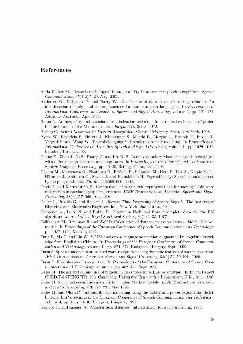
References
Adda-Decker M. Towards multilingual interoperability in automatic speech recognition. SpeechCommunication, 35(1-2):5–20, Aug. 2001.
Andersen O., Dalsgaard P. and Barry W. On the use of data-driven clustering technique foridentification of poly- and mono-phonemes for four european languages. In Proceedings ofInternational Conference on Acoustics, Speech and Signal Processing, volume 1, pp. 121–124,Adelaide, Australia, Apr. 1994.
Baum L. An inequality and associated maximization technique in statistical estimation of proba-bilistic functions of a Markov process. Inequalities, 3:1–8, 1972.
Bishop C. Neural Networks for Pattern Recognition. Oxford University Press, New York, 1998.Byrne W., Beyerlein P., Huerta J., Khudanpur S., Marthi B., Morgan J., Peterek N., Picone J.,
Vergyri D. and Wang W. Towards language independent acoustic modeling. In Proceedings ofInternational Conference on Acoustics, Speech and Signal Processing, volume II, pp. 1029–1032,Istanbul, Turkey, 2000.
Chang E., Zhou J., Di S., Huang C. and Lee K.-F. Large vocabulary Mandarin speech recognitionwith different approaches in modeling tones. In Proceedings of the International Conference onSpoken Language Processing, pp. 16–20, Beijing, China, Oct. 2000.
Cheour M., Martynova O., Naatanen R., Erkkola R., Sillanpaa M., Kero P., Raz A., Kaipio M.-L.,Hiltunen J., Aaltonen O., Savela J. and Hamalainen H. Psychobiology: Speech sounds learnedby sleeping newborns. Nature, 415:599–600, 2002.
Davis S. and Mermelstein P. Comparison of parametric representations for monosyllabic wordrecognition in continously spoken sentences. IEEE Transactions on Acoustics, Speech and SignalProcessing, 28(4):357–366, Aug. 1980.
Deller J., Proakis G. and Hansen J. Discrete-Time Processing of Speech Signals. The Institute ofElectrical and Electronics Engineers Inc., New York, 2nd edition, 2000.
Dempster A., Laird N. and Rubin D. Maximum likelihood from incomplete data via the EMalgorithm. Journal of the Royal Statistical Society, 39(1):1–38, 1977.
Falkhausen M., Reininger H. and Wolf D. Calculation of distance measures between hidden Markovmodels. In Proceedings of the European Conference of Speech Communicationn and Technology,pp. 1487–1490, Madrid, 1995.
Fung P., Ma C. and Liu W. MAP-based cross-language adaptation augmented by linguistic knowl-edge from English to Chinese. In Proceedings of the European Conference of Speech Communi-cation and Technology, volume II, pp. 871–874, Budapest, Hungary, Sept. 1999.
Furui S. Speaker independent isolated word recognition using dynamic features of speech spectrum.IEEE Transactions on Acoustics, Speech and Signal Processing, 34(1):52–59, Feb. 1986.
Furui S. Flexible speech recognition. In Proceedings of the European Conference of Speech Com-munication and Technology, volume 4, pp. 352–359, Sept. 1995.
Gales M. The generation and use of regression class trees for MLLR adaptation. Technical ReportCUED/F-INFENG/TR. 263, Cambridge University Engineering Department, U.K., Aug. 1996.
Gales M. Semi-tied covariance matrices for hidden Markov models. IEEE Transactions on Speechand Audio Processing, 7(3):272–281, May 1999.
Gales M. and Olsen P. Tail distribution modelling using the richter and power exponential distri-butions. In Proceedings of the European Conference of Speech Communication and Technology,volume 4, pp. 1507–1510, Budapest, Hungary, 1999.
Gariepy R. and Ziemer W. Modern Real Analysis. International Tomson Publishing, 1994.
48

REFERENCES
Gauvain J.-L. and Lee C.-H. Maximum a posteriori estimation for multivariate Gaussian mixtureobservations of Markov chains. IEEE Transactions on Speech and Audio Processing, 2(2):291–298, Apr. 1994.
Gold B. and Morgan N. Speech and Audio Signal Processing: Processing and Perception of Speechand Music. John Wiley & Sons, Inc., New York, 2000.
Haeb-Umbach R. Automatic generation of phonetic regression class trees for MLLR adaptation.IEEE Transactions on Speech and Audio Processing, 9(3), Mar. 2001.
Hariharan R. Robust Signal Parametrisation Techniques for Speech Recognition. Dr. Tech. thesis,Tampere University of Technology, Publications 317, Finland, 2001.
Harju M., Salmela P., Leppanen J., Viikki O. and Saarinen J. Comparing parameter tying tech-niques for multilingual acoustic modelling. In Proceedings of the European Conference of SpeechCommunication and Technology, pp. 2729–2732, Aalborg, Denmark, Sept. 2001.
Imperl B. and Horvat B. The clustering algorithm for the definition of multilingual set of contextdependent speech models. In Proceedings of the European Conference of Speech Communicationand Technology, pp. 887–890, Budabest, Hungary, 1999.
Jelinek F. Statistical Methods for Speech Recognition. The MIT Press, Cambridge, MA, 1998.Johnson R. and Wichern D. Applied Multivariate Statistical Analysis. Prentice-Hall, Inc., Upper
Saddle River, NJ, 4th edition, 1998.Juang B.-H. and Rabiner L. A probabilistic distance measure for hidden Markov models. AT&T
Technical Journal, 64(2):391–408, 1985.Junqua J.-C. Robust Speech Recognition in Embedded System and PC Application. Kluwer
Academic Publishers Group, Boston, 2000.Karjalainen M. Kommunikaatioakustiikka. Technical Report 51, Helsinki University of Technol-
ogy, Laboratory of Acoustics and Audio Signal Processing, Espoo, Finland, 1999. Preprint, InFinnish.
Kiss I. On Speech Recognition In Mobile Communications. Dr. Tech. thesis, Tampere Universityof Technology, Publications 326, Finland, 2001.
Kullback S. Information Theory and Statistics. Dover Publications, New York, 1968.Kohler J. Language adaptation of multilingual phone models for vocabulary independent speech
recognition tasks. In Proceedings of International Conference on Acoustics, Speech and SignalProcessing, volume 1, pp. 417–420, Seattle, WA, May 1998.
Kohler J. Comparing three methods to create multilingual phone models for vocabulary inde-pendent speech recognition tasks. In Proc. ESCA-NATO Tutorial and Research Workshop:Multi-lingual Interoperability in Speech Technology, pp. 79–84, Sept. 1999.
Kohler J. Erstellung einer statistisch modellierten multilingualen Lautbibliotek fur die Spracherken-nung. PhD thesis, der Technischen Universitat Munchen, 2000. In German.
Kohler J. Multilingual phone models for vocabulary-independent speech recognition tasks. SpeechCommunication, 35(1-2):21–30, Aug. 2001.
Ladefoged P., Local J. and Shockey L., editors. Handbook of the International Phonetic Associa-tion: A Guide to the Use of the International Phonetic Alphabet. Cambridge University Press,U.K., 1999.
Laurila K. Robust Speech Recognition Methods for Voice Dialing. Dr. Tech. thesis, TampereUniversity of Technology, Publications 298, Finland, 2000.
Lee L.-S. Voice dictation of Mandarin Chinese. IEEE Signal Processing Magazine, 14(4):63–101,July 1997.
Leggetter C. and Woodland P. Speaker adaptation of HMMs using linear regression. TechnicalReport CUED/F-INFENG/TR. 181, Cambridge University Engineering Department, U.K., June1994.
Leggetter C. and Woodland P. Flexible speaker adaptation using maximum likelihood linear re-gression. In Proceedings of the European Conference of Speech Communication and Technology,pp. 1155–1158, Madrid, Spain, 1995.
Leppanen J., Salmela P., Harju M., Parssinen K., Viikki O. and Saarinen J. Language adapta-tion of multilingual recognition system using MAP and MLLR. In Proceedings of InternationaConference on Speech Processing, volume 1, pp. 87–92, Taejon, Korea, Aug. 2001.
MAT. Using Matlab (Revised for Matlab 5.3, Release 11). The MathWorks Inc., 1999.
49

REFERENCES
Muthusamy Y., Barnard E. and Cole R. Reviewing automatic language identification. IEEE SignalProcessing Magazine, 11(4):33–41, Oct. 1994.
Muthusamy Y., Cole R. and Oshika B. The OGI multi-language telephone speech corpus. InProceedings of the International Conference on Spoken Language Processing, volume 2, pp.895–898, Banff, Alberta, Canada, Oct. 1992.
Navratil J. Spoken language recognition—a step toward multilinguality in speech recognition.IEEE Transactions on Speech and Audio Processing, 9(6):678–685, Sept. 2001.
Rabiner L. A tutorial on hidden Markov models and selected applications in speech recognition.Proceedings of the IEEE, 77(2):257–286, Feb. 1989.
Rabiner L. Fundamentals of Speech Recognition. PTR Prentice-Hall Inc., New Jersey, 1993.Raimo I. and Savela J. Personal communication. Department of Phonetics, University of Turku,
Finland, 2001.Reynolds D., Quatieri T. and Dunn R. Speaker verification using adapted Gaussian mixture models.
Digital Signal Processing, 10(1):19–41, Jan. 2000.Ross S. Stochastic Processes. John Wiley & Sons, Inc., New York, 1983.Rossing T. The Science of Sound. Addison-Wesley Publishing Company, Reading, Massachusetts,
2nd edition, 1990.Rosti A.-V. and Gales M. Generalised linear Gaussian models. Technical Report CUED/F-
INFENG/TR. 420, Cambridge University Engineering Department, U.K., Nov. 2001.SAM. ESPRIT project 2589: Final report – year three. Technical Report SAM-UCL-G004,
University College London, Department of Phonetics and Linguistics, England, 1989. URLhttp://www.phon.ucl.ac.uk/home/sampa/home.htm.
Schultz T. and Waibel A. Polyphone decision tree specialization for language adaptation. InProceedings of International Conference on Acoustics, Speech and Signal Processing, volume 3,pp. 1707–1710, Istanbul, Turkey, June 2000.
Schultz T. and Waibel A. Experiments on cross-language acoustic modeling. In Proceedings ofthe European Conference of Speech Communication and Technology, pp. 2721–2724, Aalborg,Denmark, Sept. 2001.
Schultz T., Westphal M. and Waibel A. The GlobalPphone project: Multilingual LVCSR withJANUS-3. In Multilingual Information Retrieval Dialogs: 2nd SQEL Workshop, pp. 20–27,Plzen, Czech Republic, Apr. 1997.
Stoica P. and Moses R. Introduction to Spectral Analysis. Prentice-Hall Inc., New Jersey, 1997.Theodoridis S. and Koutroumbas K. Pattern Recognition. Academic Press, San Diego, CA, 1999.Turunen E. Survey of theory and applications of Lukasiewicz-Pavelka fuzzy logic. In di Nola A. and
Gerla G., editors, Lectures on Soft Computing and Fuzzy Logic. Advances in Soft Computing,pp. 313–337. Physica-Verlag, Heidelberg, 2001.
Uebler U. Multilingual speech recognition in seven languages. Speech Communication, 35(1-2):53–69, Aug. 2001.
Van Compernolle D. Recognizing speech of goats, wolves, sheep and . . . non-natives. SpeechCommunication, 35(1-2):71–79, Aug. 2001.
Vihola M., Harju M., Salmela P., Suontausta J. and Savela J. Two dissimilarity measures for HMMsand their application in phoneme model clustering. Accepted to Proceedings of InternationalConference on Acoustics, Speech and Signal Processing, Orlando, USA, 2002.
Viikki O. Adaptive Methods for Robust Speech Recognition. Dr. Tech. thesis, Tampere Universityof Technology, Publications 257, Finland, 1999.
Viikki O., Kiss I. and Tian J. Speaker- and language-independent speech recognition in mobilecommunication systems. In Proceedings of International Conference in Acoustics, Speech andSignal Processing, volume I, pp. 5–8, Salt Lake City, Utah, May 2001.
Viikki O. and Laurila K. Cepstral domain segmental feature normalization for noise robust speechrecognition. Speech Communication, 25(1-3):133–147, Aug. 1998.
Viterbi A. Error bounds for convolutional codes and an asymptotically optimum decoding algo-rithm. IEEE Transactions on Information Theory, 13:260–267, 1967.
Waibel A., Geutner P., Tomokiyo L., Schultz T. and Woszczyna M. Multilinguality in speech andspoken language systems. Proceedings of the IEEE, 88(8), Aug. 2000.
50

REFERENCES
Winski R. SpeechDat: Definition of corpus, scripts and standards for fixed networks. TechnicalReport LE2-4001-SD1.1.1, http://www.speechdat.org/, Jan. 1997.
Woodland P. and Young S. The HTK tied-state continuous speech recogniser. In Proceedings ofthe European Conference of Speech Communication and Technology, volume 3, pp. 2207–2210,Berlin, 1993.
Young S., Adda-Decker M., Aubert X., Dugast C., Gauvain J.-L., Kershaw D., Lamel L.,Leeuwen D., Pye D., Robinson A., Steeneken H. and Woodland P. Multilingual large vocabu-lary speech recognition: The European SQALE project. Computer Speech and Language, 11(1):73–89, 1997.
Young S., Kershaw D., Odell J., Ollason D., Valtchev V. and Woodland P. The HTK Book (forHTK Version 3.0). Cambridge University Engineering Department, U.K., July 2000.
Young S., Russell N. and Thornton J. Token passing: A simple conceptual model for connectedspeech recognition systems. Technical Report CUED/F-INFENG/TR. 38, Cambridge UniversityEngineering Department, U.K., July 1989.
Zgank A., Imperl B. and Johansen F. Crosslingual speech recognition with multilingual acousticmodels based on agglomerative and tree-based triphone clustering. In Proceedings of the Euro-pean Conference of Speech Communication and Technology, pp. 2725–2728, Aalborg, Denmark,Sept. 2001.
51

Appendix A
Transformation Classes for MLLR
In the MLLR adaptation framework, discussed in Chapter 2, the target densities areassigned into transformation classes to ensure the sufficient data to estimate the transformmatrices. All the densities in one transformation class are assumed to have similar acousticproperties, as they are transformed using a common transformation matrix [Leggetter andWoodland 1994]. Usually a transformation class tree is built to enable dynamic use ofthe transformation classes. This means that the more adaptation data is available, themore specific transforms can be used [Leggetter and Woodland 1995]. An example ofthe transformation class tree is exemplified in Figure A.1. This transformation class tree isusually built either by using phonetic knowledge, or by some acoustic clustering algorithm.
The dissimilarity measures, discussed in Chapter 4, can also be employed for the definitionof the transformation class tree. The Sections A.1 and A.2 briefly describe the differentmethods that have been used for defining a transformation class tree. The Section A.1describes some acoustic clustering algorithms that form a tree consisting of the mixturecomponents of the state-dependent densities of HMMs. The Section A.2 discusses theHMM level definition of the transformation class tree. Most commonly used method fordefining a HMM level transformation class tree is the phonetic knowledge, but also acomputational method has been proposed [Haeb-Umbach 2001].
A.1 Mixture Component Level Definition
Some acoustic clustering algorithms used in the definition of the transformation classesutilize a distance measure between two mixture components. Based on the measure, atree of mixture component classes can be created using e.g. the agglomerative clusteringscheme shown in Algorithm 3.1. The advantages of this method are that expert phoneticknowledge is not needed, and the construction of the tree can be done using the availableadaptation data [Leggetter and Woodland 1995, Young et al. 2000]. The disadvantage ofthis mixture component level method is that the mixture components of a single HMM, oreven state, can be transformed using several different transformation matrices [Leggetterand Woodland 1994].
The acoustic clustering method used by Leggetter and Woodland employed the Kullback-Leibler divergence between two Gaussian mixture density components as a distance mea-sure [Leggetter and Woodland 1995]. The algorithm implemented in Hidden Markov ModelToolkit (HTK) introduces occupation counters1 in addition to the KL divergence to create
1. The occupation counters are the mean number of feature vectors that are assigned to a particularmixture component. They can be obtained using the posteriori probabilities γt(j, k) defined in Section 2.4.3.
52

APPENDIX A. TRANSFORMATION CLASSES FOR MLLR
1
2 3
4 5 6 7
8 9
Figure A.1: An example of a transformation class tree that may be used in MLLR adap-tation. Gray circles denote nodes with insufficient data. In this example, onlythree transformation matrices are computed: for nodes 2, 3 and 7. The compo-nents in terminal nodes (TNs) 8, 9 and 5 are transformed using one commontransformation matrix. The TN 7 has its own specific transformation, and thecomponents in TN 6 are transformed with a transformation matrix calculatedusing the data from both TNs 6 and 7.
the transformation classes [Young et al. 2000]. This enables the creation of such clustersthat utilize the specific adaptation data more efficiently. Gales has proposed a method thatis optimal in the sense of maximizing the likelihood of the transformation class usage. Theresults, however, differed very little from the acoustic clustering used as a baseline [Gales1996]. Furthermore, this method is computationally expensive.
A.2 HMM Level Definition
The use of phonetic knowledge in the generation of transformation class tree ensuresthat all the mixture component densities in one HMM are transformed using a commontransform matrix [Leggetter and Woodland 1994]. The disadvantage of this method is theuse of expert knowledge which may not be available. Moreover, the phonetic trees are notunique as the phonetic categories are not strictly hierarchical [Raimo and Savela 2001].An example of a phonetic transformation class tree is shown in Figure A.2.
The dissimilarity measures presented in Chapter 4 could be also used to define a trans-formation class tree in HMM level. The agglomerative clustering procedure described inAlgorithm 3.1 produces a binary tree [Theodoridis and Koutroumbas 1999]. The questionof using dissimilarity measures for HMMs for defining a transformation class tree is out ofthe scope of this thesis, but is mentioned here for possible future work. A computationalHMM level transformation class tree definition has been reported earlier in [Haeb-Umbach2001]. The dissimilarity measure employed in that research was based on inter-speakercorrelation [Haeb-Umbach 2001]. The advantages of this type of transformation class treedefinition is the HMM level definition, which has been mentioned as an advantage of thephonetic transformation class tree definition.
53
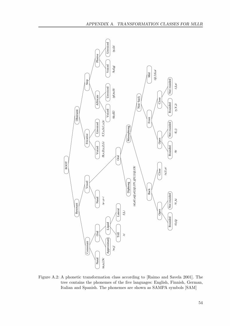
APPENDIX A. TRANSFORMATION CLASSES FOR MLLR
Obs
true
nt
/r/
Nas
al
/p,t,
k//b
,d,g
//d
z,dZ
//p
f,ts,
tS/
/B,v
,D,z
,Z,G
//f,
T,s
,S,C
,x,h
/
Voi
ced
Unv
oice
dV
oice
dU
nvoi
ced
Affr
icat
eP
losi
ve
Fric
ativ
e
Voi
ced
Unv
oice
d
Con
sona
nt
App
roxi
man
t Tril
lLa
tera
l
Liqu
id
Vow
el
Res
onan
t Nas
al
Mid
/@,3
,6,a
/
Mon
opht
ong
Dip
hton
g
Clo
seO
pen
Rou
nded
Not
rou
ndedBac
k
/V,A
/
/u,U
,o/
Fro
nt
Clo
seO
pen
Rou
nded
Not
rou
nded
Rou
nded
Not
rou
nded
Non
−ba
ck
Ora
l
/m,n
,J,N
/
Ora
l
/a~
,o~
/
RO
OT
Sto
p
/l,L/
/9/
/O,Q
//i,
I,e/
/y,Y
,2/
/E,{
/
/w,j/
/aI,a
U,e
@,e
I,I@
,OY
,@U
,U@
,OI/
Figure A.2: A phonetic transformation class according to [Raimo and Savela 2001]. Thetree contains the phonemes of the five languages: English, Finnish, German,Italian and Spanish. The phonemes are shown as SAMPA symbols [SAM]
54