Displacement and Development: Long Term Impacts

of Population Transfer in India ∗

Prashant Bharadwaj† Rinchan Ali Mirza‡

August 2018

Abstract

The partition of British India in 1947 resulted in one of the largest and most

rapid migrations and population transfers of the 20th century. Using refugee pres-

ence by 1951 as a measure for the intensity of the impact of the population transfer,

and district level data on agricultural output between 1911-2009 from India, we find

using difference in differences and event study approaches that areas that received

more refugees have higher average yields, are more likely to take up high yielding

varieties of seeds, and are more likely to use agricultural technologies. The increase

in yields and use of agricultural technology coincide with the timing of the Green

Revolution in India. Using pre-partition data, we show that refugee placement is

uncorrelated with soil and water table characteristics, agricultural infrastructure,

and agricultural yields prior to 1947; hence, the effects are not explained by selec-

tive movement into districts with a higher potential for agricultural development.

We highlight refugee literacy and land reforms in areas with refugees as two of the

many potential mechanisms that could be driving these effects.

JEL Codes: O13, O33, O15, Q16, N55

∗This project has benefitted from comments by Latika Chaudhary, James Fenske, Bishnupriya Gupta,Asim Khwaja, Takashi Kurosaki, Atif Mian, participants of the 17th World Economic History Congress,organizers and participants of the 10th International Conference on Migration and Development, andvarious seminar participants.†University of California San Diego & NBER. Corresponding author: Economics Dept, 9500 Gilman

Dr. #0508, La Jolla, CA 92093-0508, US. Phone: +1-858-822-6760. E-mail: prbharadwaj@ucsd.edu‡Namur University, Belgium. Website: www.rinchanmirza.com

1

1 Introduction

The end of the British Empire in India in 1947 was marked with an unprecedented

mass migration and population transfer of nearly 17 million people. By many accounts

this was a human rights disaster involving nearly a million deaths due to the riots that

ensued between Hindus and Muslims on either side of the newly created India-Pakistan

border. As historical events undoubtedly shape modern day institutions and economic

development (Acemoglu, Hassan, and Robinson, 2011; Nunn, 2008; Banerjee and Iyer,

2005; Acemoglu, Johnson, and Robinson, 2002; Chaney and Hornbeck, 2015; Dippel,

2014; Dell, 2010), one can only imagine whether and how the emergence from nearly a

century of colonial rule left an indelible mark on Indian economic progress.1 This paper

seeks to examine the legacy of the migration and population transfer that took place at

partition on an important aspect of economic progress – agricultural development.

This paper shows that areas that received refugees do better in the long run in terms

of agricultural development. Documenting this relationship is an important contribution

as mass migrations, institutional upheaval, and partitions are a reality even today.2 It is

therefore crucial to understand how communities and areas develop long after such events

take place. While almost by definition affected areas suffer in the short run, it is critical

to document whether the legacy of such events forever change the long run trajectory of

these places.

We find that areas that received a high fraction of refugees by 1951 have significantly

higher yields compared to areas with low fraction of refugees in the decades after India’s

independence. Between 1957 and 2009, districts that had a greater refugee presence saw

average annual wheat yields increase by 9.4% compared to low refugee districts. We find

similar results when examining annual revenue per hectare.3 The take off in agriculture

1Data limitations prevent us from examining these impacts on the Pakistani side.2The recent (as of September 2017) refugee crisis in Europe is a relevant example of a mass migration

with the potential to affect labor markets and economic development of receiving countries. The mostrecent example of a partition is that of Sudan where in a referendum held in January 2011 in the southshowed that an overwhelming 98.8 percent of the population were in favor of secession. As a consequence,constitutional declaration of the independence of South Sudan took place on 9 July 2011. The otherrecent example is the Dayton peace agreement of November 1995, which led to the partition of Bosniaand brought an end to the Bosnian War. Yet another prominent example is the partition of Cyprusinto Greek and Turkish speaking separate territorial units after the Turkish invasion and occupation ofNorthern Cyprus in 1974 (Christopher, 2011; Kumar, 2004; Kliot and Mansfield, 1997).

3This measure is used so as to not be reliant on any specific crop for our productivity measures.The measure uses data on the production of wheat, rice, sugar, jowar, maize, bajra, barley, cotton,

2

in refugee settled areas occurs at the same time as the green revolution starts in India.

The green revolution transformed Indian agriculture in the 1960s, making crops less

susceptible to destruction via pests and droughts, increasing yields, and increasing land-

based investments like irrigation. We find that refugee presence is strongly correlated

with the use of tractors (going from a low refugee district to a high refugee district

increases the use of tractors by 56% between 1957-1987) and fertilizers (phosphorous and

nitrogen).

A key aspect of our empirical framework uses agricultural data from before 1951, and

employs a difference in differences design for a subset of districts for whom such data is

available to examine the impact of partition affected districts on long run agricultural

outcomes. A concern with examining simple correlations of refugee presence and outcomes

is that despite the uncertainty and chaos of partition, refugees might have moved to places

pre-disposed to agricultural growth. Hence, the ability to use extensive pre-partition

agricultural data goes a long way in ensuring that districts that were affected by partition

related migration are not on differential trends until the start of the green revolution.

While limited in our ability to examine trends along certain other variables, we use

available data to examine at least in levels whether refugees went to more endowed

districts along dimensions that might matter for agricultural development. For example,

canals and tube wells were important characteristics that allowed for the spread of high

yielding varieties of seeds; however, we find no correlation between pre-partition canal

irrigation, aquifer depth in districts (groundwater access has been shown to be a strong

predictor of the green revolution – see D’Agostino (2017)), and refugee presence. We also

find no correlation between refugee migration and the presence of other infrastructure

variables such as banks, post offices, length of roads, and hospitals by 1961 (pre green

revolution). This mitigates the concern that even if migrants did not choose districts

based on agricultural yields, they might have chosen districts based on some characteristic

that happened to be extremely important for the spread of the green revolution (like

roads, banks, or schooling).

However, we might still be concerned that refugee presence might be generally related

to district characteristics or trends that affect agricultural yields. Our results on refugee

presence and yields are however only present for crops that were affected by the green

revolution. Non green revolution crops, such as millets, chickpeas, rapeseed etc. do not

groundnut, jute gram, potato, ragi, rapeseed, mustard, sesame, soybean, sugarcane, sunflower, tobacco,tur and other pulses.

3

show any changes in yields with refugee presence. Our results are also robust to restricting

the sample to just the two north-western states of United Provinces and Punjab. United

Provinces and Punjab are the two states that bore the brunt of the partition-related

violence and where refugees were resettled successfully shortly after partition. They form

the main focus of our study. Finally, we are able to account for an important institutional

feature of the British colonial system that has been shown to affect agricultural yields and

the take up of the green revolution - the British taxation system on agricultural lands.

Using data from Banerjee and Iyer (2005), we are able to control for these features, and

find that adding these controls does not affect our main estimates.

While we believe these results to be important, we want to be upfront about the scope

and limitations of this paper. This research is motivated by the goal of linking partition to

subsequent economic development (as measured by income, health and human capital);

however, in this paper we specifically (and only) examine agricultural outcomes. There

are two main reasons for this: first, agricultural outcomes are available at a yearly level,

at fine levels of administrative disaggregation, and over a long period of time – the same

is not true of many other variables of interest to development economists like health,

income, etc. Second, agriculture was, and still is, an important part of employment and

economic output in India.4

A second limitation of this study is that the partition was an event that resulted in many

changes: two way migrations along two new borders, new governments, mass deaths,

demographic changes, increased religious homogeneity, and loss and restructuring of land,

just to name a few. Hence, our interpretation of the results is that areas (districts in

our case) that received refugees due to partition were more “affected” along various

dimensions, like the ones we just mentioned, by partition than districts that did not

receive any refugees.5 While we use the refugee population as our metric for the intensity

of the impact of partition, it would be incorrect to interpret our results as solely the

effects of partition induced migration. For example, districts with more refugees could

4In 2014 approximately 17 percent of Indian GDP was made up of the agricultural sector and forthe decade prior to that it fluctuated between 18 and 17 percent. In 2012 as much as 47 percent of thetotal Indian workforce was employed in agriculture (data from World Bank Economic Indicators).

5Note that this also comes with an important interpretation when studying the impacts of migrationor refugee flows that “more” refugees implies higher intensity of impact – this is only true if the compo-sition of migrations in areas with “more” migrants is the same as the composition of migrants in areaswith “less” migrants. If more educated (but fewer in number) refugees travel further then just usingrefugee numbers is not adequate to measure impact. While it is entirely plausible that different typesof refugees ended up in Tamil Nadu relative to the Punjab, the fact that we use state fixed effects andexamine variation in refugee settlements across districts but within a state mitigates this concern.

4

have received more government aid in the years after partition, and our effects should be

interpreted as capturing the reduced form effect of both refugee presence and government

assistance. We wish to point out that this issue is present in all studies of mass migrations.

Mass migrations or refugee movements, by their very nature, induce all kinds of responses

on the part of sending and receiving governments and communities. At its core, this paper

is a reduced form way of understanding how places that were affected by the partition

related population transfer fare in the long run.

Data limitations, the sheer magnitude of the event, and the two way nature of the refugee

flows therefore makes it nearly impossible to make precise statements about any one

leading factor. We do, however, provide some preliminary evidence that the composition

of refugees played a qualitatively important role in the future agricultural development

of more affected areas. Migrants who moved to India were more educated than the

natives who stayed behind (Bharadwaj, Khwaja, and Mian, 2009). Given the positive

correlation between education and the better use and take up of agricultural technologies

(Feder, Just, and Zilberman, 1985), the demographic changes induced by partition could

be a plausible mechanism for the effects seen. These findings are also consistent with the

seminal work of Foster and Rosenzweig (1996).

We explore two other mechanisms, but provide more qualitative evidence towards these.

First, the data show that refugees were more likely to have been involved in money

lending and other commercial aspects of farming. Since credit is an important aspect of

agriculture and especially so for the take up of newer technologies it is likely that the

presence of refugees during the green revolution helped along this dimension. Second,

the way land was redistributed to refugees likely resulted in more land consolidation

and redistribution in areas that had more refugees. If consolidated lands were more

likely to see investments in technology during the green revolution, then this could be

an important channel for the results. While we do not have data on farm size before

and after partition at the district level, we provide qualitative evidence towards this

mechanism. We hope future research in this area can shed empirical evidence towards this

mechanism. Finally, since partition resulted in two way migration flows (Muslims leaving

India, replaced by Hindus and Sikhs arriving from Pakistan/East Pakistan) resulting in

no major net population change at the district level in India, the main mechanism for

agricultural development is unlikely to be the same as identified by Hornbeck and Naidu

(2014) in the case of the American South, or the local agglomeration effects in West

Germany studied by Peters (2017). We are well aware that the mechanisms we explore

5

are neither conclusive nor exhaustive. However, even identifying the reduced form impacts

of refugee movements poses significant challenges (both in terms of data and econometric

identification) and we leave the deep exploration of individual mechanisms to future work.

This paper contributes to the economics literature on the long term impacts of historical

events in general (see Nunn (2009) for a review), and also to the literature more focussed

on the impacts of history and colonization in India (Jha, 2013; Chaudhary and Rubin,

2011; Donaldson, 2010; Iyer, 2010). Most closely related is the work of Banerjee and Iyer

(2005), who show that different institutions (specifically practices regarding land rights)

during the colonial period had a profound impact on agricultural development long after

the British left India. They find that these institutions played an important role after

the green revolution, where individual rights to ownership of land were a crucial aspect of

districts that were able to take advantage of HYV seeds, fertilizers, and other agricultural

technologies. This paper also builds on and extends the research that is directly related

to the partition of India (Bharadwaj, Khwaja, and Mian, 2009; Jha and Wilkinson, 2012;

Bharadwaj and Fenske, 2012). While these papers contribute in important ways to our

understanding of the event by analyzing the demographic consequences of partition, the

role of combat experience during WWII on ethnic cleansing during the partition, and

the impact of partition related migratory movement on jute cultivation, they do not

examine long run consequences. Hence, the main contribution of this work is to examine

how partition (as measured by the presence of refugees) impacted long run economic

outcomes such as agricultural development.

2 Background

2.1 Partition of India

Although the possibility that British India would be partitioned upon independence had

been present for several years prior to the actual event, the partition when it finally

came on August the 14th, 1947 was sudden, violent and chaotic for the millions who

found themselves on the wrong side of the newly created India-Pakistan border. An

estimated 14.5 million people were displaced within a short span of just four years after

partition (Bharadwaj, Khwaja, and Mian, 2008, p. 39). As the partition was based along

religious lines the dominant factor behind migratory flows was religion. Muslims who

found themselves a minority in India had to move to Pakistan. On the other hand the

6

Hindu and Skih minorities of Pakistan were forced to move to India. Those districts that

experienced greater out-flow of peoples also received more inflows. Bharadwaj, Khwaja,

and Mian (2008) call such a pattern the “replacement effect”. They also document what

they term is a “distance to the border effect” whereby districts that were closer to the

partition border experienced both greater inflow and outflow of peoples.

An important contribution of the Bharadwaj, Khwaja, and Mian (2009) study is to

highlight the demographic consequences of partition. They document a shift in the de-

mographic make-up of districts that experienced greater inflow and outflow of peoples

along three dimensions: education, occupation and gender. In particular, their results

show that refugees were more likely to be “educated, and choose non-agricultural profes-

sions” (Bharadwaj, Khwaja, and Mian, 2009, p. 2). A one standard increase in refugees

inflows and outflows led to a 0.9% increase in literacy in India and a 1.16% increase in

persons engaged in non-agricultural occupations. Since, it was the religious minority on

both sides of the border who were forced to move the partition led to a significant de-

cline in religious diversity. The drop in diversity was particularly stark along the western

border. The percentage of Muslims fell from 30 per cent to 1.75 per cent in districts that

later became Indian Punjab. “Similarly, in the districts that became part of Pakistani

Punjab, the percentage of Hindus/Sikhs fell from 21.7 per cent to [just] 0.16 per cent!”

(Bharadwaj, Khwaja, and Mian, 2008, p. 40).

The decision to partition was formally laid out by the British in the shape of a plan on

June the 3rd, 1947. The partition plan, as it was called, laid the foundations for redrawing

the boundaries of the two most contested states of Punjab and Bengal. A British civil

servant, Cyril Radcliffe, was appointed chairman of the Punjab and Bengal boundary

commissions. Radcliffe was both unfamiliar with boundary making and had no intimate

knowledge of the people or the land he was about to carve up (Yong and Kudaisya, 2000,

p. 84). His task was further complicated by the procedural difficulties involved in the

partition plan itself. While all major political parties had agreed upon partition, they had

vaguely laid down that boundaries would be demarcated by contiguous majority areas of

Muslims and Non-Muslims as well as by considering “other factors”. This clause – “other

factors” – probably caused the most controversy during the entire process of boundary

making. The idea of “contiguous areas” was also vague as it was not certain whether this

meant districts or tehsils or other, smaller, administrative units.

Further adding to the chaos and confusion surrounding partition was the fact that Rad-

cliffe’s decision regarding the placement of the partition border was kept secret until the

7

very last minute. Such secrecy heightened speculation regarding his methods of demar-

cating the border. It was alleged that Radcliffe used the 1941 census to calculate religious

majorities in various districts. Since the decision for a separate Muslim state was released

in 1940, many feared that the 1941 census was rigged and under reported the presence

of certain religious groups.

The reports of the boundary commissions were eventually made public on August 17th,

1947, two days after India had declared her independence. Immediately afterwards there

were voices of dissent coming from all quarters. The myriad factors that Radcliffe had to

consider in a short period of time, made the placement of the partition border both illogi-

cal and inconsistent. The border “zigzagged precariously across agricultural land, cut off

communities from their sacred pilgrimage sites, paid no heed to railway lines or the in-

tegrity of forests, [and] divorced industrial plants from the agricultural hinterlands where

raw materials, such as jute, were grown” (Khan, 2017, p. 126). Once the partition line

was revealed, thousands found themselves on the wrong side of the border, particularly

in the state of Punjab. There were neither provisions nor preparations for the affected

populations to be evacuated, until it was too late (Yong and Kudaisya, 2000, p. 98). The

ensuing violence, migrations and human suffering were unprecedented. Even before the

declaration of independence, the violence in both Punjab and Bengal had started to take

its toll with several incidents of rioting between the Muslims on one side and Hindus and

Sikhs on the other.

Considered together, the above factors point to certain features of the partition that

are important to the context of our paper. First, areas from where there was greater

outflow of peoples also experienced greater inflows (“replacement effect”). Second, areas

closer to the partition border saw greater outflows as well as inflows (“distance to border

effect”). Third, the partition led to significant shifts in the demographic make-up of

areas that were most affected. In areas that saw greater inflows and outflows there

was an overall improvement in literacy and an increase in the non-agricultural share of

the labour force. Fourth, the rapidity with which the partition unfolded meant that

the majority of migratory flows took place under a relatively short span of time and

without much preparation. Fifth, since the boundaries were not declared till later and

there was a lot of uncertainty regarding them, it was unlikely that people moved much

before partition. Finally, the fact that the partition plan was riddled with procedural

difficulties and inherent contradictions meant that the border line was drawn without

paying adequate attention to the economic and geographic factors on the ground.

8

2.2 East Punjab Refugee Resettlement

A monumental task faced by administrators immediately after independence was to re-

settle refugees who had arrived from Pakistan as quickly as possible so as to minimize

the disruption caused by partition. The way in which the refugee resettlement process

unfolded, however, differed fundamentally between the Western and Eastern borders.

Along the Western border, refugees were quickly resettled through a means of a centrally

organized plan that was executed effectively by willing administrators. In contrast, for

the Eastern border there was neither a plan nor the willingness on behalf of adminis-

trators to resettle refugees in large numbers. In fact, the post independence government

of West Bengal made every attempt to avoid a population exchange between East and

West Bengal and was caught completely unprepared by the extent of the refugee crisis in

its state around partition. As a consequence many of the refugees who arrived in West

Bengal ended up not being resettled at all. Accordingly, we have only discussed the East

Punjabi refugee resettlement process, the main focus of our study, in the main text of

our paper and have moved the discussion of what happened to refugees who came from

East Bengal to Appendix B.

The resettlement of refugees in East Punjab was both short and largely successful. On

15 September 1947, just one month after Partition, the East Punjab government decided

that “rural refugees should be temporarily settled on evacuee land and that each family

be given a plough unit” (Kudaisya, 1995, p. 77). In late 1949, the scheme of permanent

allotment of evacuee land to refugees was ready for implementation (Kudaisya, 1995,

p. 81). The East Punjab government completed implementation of the permanent al-

lotment scheme in early 1951 by delivering evacuee land to refugees (Kudaisya, 1995,

p. 81). The swiftness and success of the resettlement process was such that “by the early

1960s the refugees had not only settled” on their allotments “but had also attained a

certain level of prosperity” (Kudaisya, 1995, p. 85). The following paragraphs describe

the process of East Punjab refugee resettlement in detail.

In the immediate aftermath of the Partition, the refugee population of East Punjab was

assigned temporary allotments of land (Kudaisya, 1995, p. 77). Under the temporary

allotments, each refugee family “was given a plough unit, i.e. about 10 acres of land,

regardless of its holdings in Pakistan” from East Punjabi villages where land had become

available because of the evacuation of the Muslim population (Randhawa, 1954, p. 67).

In assigning temporary allotments, the government made no distinction between refugees

9

who had been tenants or landholders. Moreover, rather than assign temporary allotments

to individuals or families, the resettlement administrators decided to assign them to

groups of families. It was not obligatory for group allottees to cultivate jointly the

area allotted to their group. Instead, if a group allottee wanted to cultivate their share

separately s/he could do so by simply asking for their share to be demarcated (Randhawa,

1954, p. 68). There were certain benefits from making ‘group’ as opposed to ‘individual’

or ‘family’ allotments. It was easier, logistically, for resettlement administrators to deal

with groups of families rather than individuals or families when assigning allotments.

Working together as a group also made it easier for refugee families to pool their resources

to secure access to agricultural inputs like bullocks and implements. Through temporary

allotments the refugees were able to take up almost the entire area left behind by Muslim

evacuees in a short span of time. Later, when the government launched the permanent

allotment scheme, a substantial number of the temporary allottees were confirmed in the

villages of their temporary allotments.

Under the scheme of temporary allotments, the East Punjab government did not con-

sider the previous land holdings of refugees. Therefore, a need arose to formulate a more

permanent scheme of allotments that would take into account the size of holdings left

behind by refugees in Pakistan. Accordingly, the government of East Punjab launched a

scheme of quasi-permanent allotments in February 1948. As part of the scheme, refugees

submitted their claims to evacuee land based on the size of their previous land holdings

in Pakistan. A total of 517,401 refugee households or families submitted their claims

during the period of March 1948 to April 1948. Once received, the claims were matched

against revenue records held by the East Punjab government on Pakistani villages evac-

uated during Partition. Whilst the claims were being processed, it became clear that a

significant proportion of the refugees had exaggerated the size of their holdings in Pak-

istan (Kudaisya, 1995, p. 79). The government therefore decided not to proceed with the

scheme of quasi-permanent allotment and instead made further efforts to develop a more

accurate assessment of past refugee land ownership. Through the involvement of village

panchayats and local land revenue staff, the government was eventually able to ‘obtain a

fairly accurate picture of the precise extent of land ownership’ of the refugees (Kudaisya,

1995, p. 79).

Building upon the work completed under the scheme of quasi-permanent allotments,

resettlement administrators devised a scheme for the permanent rehabilitation of refugees

(Kudaisya, 1995, p. 79). Administrators faced two important issues when devising such a

10

scheme. The first was to resettle refugees across areas that varied greatly in terms of soil,

irrigation, rainfall and productivity. To facilitate the allotment of evacuee land across

agriculturally diverse areas, the administrators created a common measure of value called

the ‘standard acre’ (Kudaisya, 1995, p. 79). The ‘standard acre’ acre was different from

the physical acre and represented a unit of value based on the productivity of the land

rather than the physical area covered by the land. For example, one physical acre that

could yield ten to eleven maunds of wheat was equivalent to a ‘standard acre’, whereas,

a physical acre that yielded only five to six maunds of wheat was equivalent to one half

of a ‘standard acre’. The diversity in agricultural conditions across East Punjab meant

that the physical area behind a standard acre varied substantially across its sub-regions.

In the dry south-eastern districts of Hissar and Gurgaon, four physical acres made one

standard acre. On the other hand, in the highly productive canal irrigated tracts of

the province, a single physical acre was equivalent to a ‘standard acre’ (Kudaisya, 1995,

p. 80). A comprehensive description of the grading system for land and its valuation in

terms of the ‘standard acre’ across each of the tehsils of East Punjab is available in Singh

(1952).

The second issue facing resettlement administrators was to determine the extent of refugee

compensation based on the size of land holdings left behind in Pakistan. To address the

issue resettlement administrators developed a system of ‘graded cuts’ as a solution (Ku-

daisya, 1995, p. 81). According to the system of ‘graded cuts’, refugee claims expressed

in ‘standard acre’ terms were placed into different categories based on the size of land

holdings left behind in Pakistan. The administrators then applied a different discount

rate, known as the ‘rate of cut’, to the claims in each size category to reach the net

allotment of land to refugees. The sliding scale applied by the administrators under the

graded cuts system to arrive at the net allotments of refugees is summarised in Figure

1. It is clear from the figure that for small claims of up to ten standard acres the ‘rate

of cut’ was 25 per cent. At the extreme end, claims upwards of 500 standard acres were

subjected to a 95 per cent ‘rate of cut’.

The above discussion points to two features of the refugee resettlement process that are

important to the context of our study. The fact that refugee resettlement was centrally

planned and managed by the state means that it is unlikely that refugees were able to

self-select into districts that were pre-disposed to great agricultural development. Further-

more, the speed and success of the permanent allotment scheme meant that most refugees

were already permanently settled by the time the 1951 census was undertaken. This is

11

Figure 1: Sliding scale used for net allotment of refugees

crucial for our refugee presence measure to reflect only permanently settled refugees who

were unlikely to have migrated later on.

2.3 Green Revolution in India

2.3.1 Development of High Yielding Varieties

The Green Revolution originates from the cross-breeding experiments carried out at the

International Rice Research Institute (IRRI), in the Philippines in 1961, and its sister

institution, the International Centre for Maize and Wheat Improvement (CIMMYT) in

Mexico in 1967. The objective of the experiments was to develop shorter, stiff strawed

varieties of the wheat and rice crops that devoted much of their energy to producing

grain and relatively little to producing straw or leaf material (Evenson and Gollin, 2003,

p. 758). The development and diffusion of HYVs of crops other than rice and wheat took

longer and was not as impressive as that of rice and wheat. This was because scientists

had already developed a critical mass of knowledge for rice and wheat in particular, which

did not exist for other crops (Evenson and Gollin, 2003). As late as the 1980s only a

few HYVs of crops like sorghum and millet had been developed (Evenson and Gollin,

2003, p. 758). The differences in the initial stock of scientific knowledge of crops meant

that the benefits of HYV adoption in terms of increasing agricultural productivity were

largely concentrated in households producing wheat and rice.

12

2.3.2 Diffusion of rice and wheat HYVs in India

A selection of the hybrid varieties developed at the IRRI and CIMMYT were imported

into India where they were further crossed with local varieties to adapt to local conditions.

Out of these crosses came the locally adapted rice varieties of “Padma” and “Jaya” and

wheat varieties of “Kalyan Sona” and “Sonalika”. It was the large scale release of such

locally adapted varieties in the late 1960s that marked the start of the Green Revolution

in India. The wheat varieties of “Kalyan Sona” and “Sonalika” were an immediate

success and were quickly adopted in the three main wheat growing regions of India:

the Northwest Plains, the Northeast Plains, and the Central Peninsular zone6. Due to

the rapid adoption of the wheat varieties, the production of wheat went up from twelve

million tons to twenty million tons between 1966-67 and 1969-70, an increase of 40% in

the span of just three years (Chakravarti, 1973, p. 321). The success of the varieties was

due to their robustness to the varying conditions under which wheat is grown in India

(Munshi, 2004, p. 187). Building on the success of the early wheat varieties, agricultural

scientists began concentrating their research on developing new varieties for what were

termed “marginal environments”. Marginal environments included low rainfall areas

with limited or no irrigation infrastructure. As a consequence of the continuing research

efforts, a new generation of wheat varieties were developed that were able to penetrate

into marginal environments in the later phases of the Green Revolution (Byerlee and

Moya, 1993, p. XI).

In contrast to the early wheat varieties, the early rice varieties of “Padma” and “Jaya”

were less successful in penetrating the rice growing areas of India. Both varieties were

unsuitable in a variety of stress conditions such as water logging, salinity and drought

(Munshi, 2004, p. 190). They were also found to be susceptible to a number of pests and

diseases prevalent in the rice growing areas (Munshi, 2004, p. 190). Due to the limited

success of the early rice varieties Indian agricultural scientists concentrated their research

efforts on developing varieties that were suited to local conditions in rice areas (Munshi,

2004, p. 190) and also incorporated resistance to pests and diseases (Evenson and Gollin,

2003, p. 759).

6The states of Punjab, Haryana, (western) Uttar Pradesh, Delhi and Rajasthan make up the North-west Plains region. The Northeast Plains region includes (eastern) Uttar Pradesh, Bihar, Orissa andBengal. Finally, the Central Peninsular zone is made up of the states of Madhya Pradesh and Gujarat.

13

The greater success of wheat HYVs relative to the rice varieties means that we focus

exclusively on wheat yields in this paper; although we do show results for all crops in an

aggregate revenue per acre measure as well.

2.3.3 Role of canals and aquifers

In addition to the differences in seed technology discussed above, there were other factors

that were important in the adoption of rice and wheat HYVs in India. One of these

was the timely and controlled provision of water (Rud, 2012, p. 353). The uninterrupted

supply of water at specific periods of growth, development and flowering was crucial to

the successful performance of the HYVs. That is why pre-existing patterns of irrigation

and climate were one of the main drivers behind their diffusion (Gollin, Hansen, and

Wingender, 2016, p. 5). The importance of irrigation can be gauged by the fact that states

like Punjab, Haryana and Tamil Nadu that had a well developed irrigation infrastructure

dating back to the colonial period rapidly adopted HYVs shortly after the start of the

Green Revolution (Evenson and Gollin, 2003b, p. 91). On the other hand, at around

the same time states like Gujarat, Maharashtra, Orissa, West Bengal, Bihar, Kerala and

Rajasthan, that lacked an extensive irrigation network, were lagging behind considerably

in terms of HYV adoption (NCAI-I, 1976, p. 284).

Beginning with the introduction of HYVs in the late 1960s, more minor irrigation projects

were undertaken to rapidly expand irrigation beyond the historically canal-irrigated

states. The minor irrigation projects used electrified tube-wells to access groundwa-

ter instead of using canals to access river water (Rud, 2012, p. 353). They offered greater

control in terms of flow and timing of water supplies compared with canal irrigation

(NCAI-V, 1976, p. 20). Due to their cost effectiveness, the minor irrigation projects were

also particularly attractive for small and medium farmers in areas without canal irriga-

tion. Recognizing the importance of minor irrigation projects the Indian state financed

the extension of the electricity network across rural India and provided credit to farmers

for purchasing electrified tube-wells (NCAI-V, 1976, p. 20). As a consequence, the use

of electrified tube-wells for groundwater irrigation accelerated remarkably after the start

of the Green Revolution in the late 1960s. It is important to note that groundwater

irrigation depends crucially on the depth of aquifers (D’Agostino, 2017). Aquifers are

underground layers of water bearing permeable rock, rock fractures or other unconsoli-

dated materials from which groundwater can be extracted. The closer an aquifer is to the

14

surface (i.e. of lower depth) the more likely it is to be used for groundwater irrigation.

Hence, in this paper we crucially account for the presence of historic canals as well as

aquifer depth in our estimations.

3 Data and Empirical Framework

3.1 Full Sample Analysis

For our full sample analysis that relates to the post-partition period the data comes from

three different sources: the 1951 census of India, the Indian Agriculture and Climate

Dataset (i.e. IACD) and the Village Dynamics in South Asia Dataset (i.e. VDSA). The

1951 census data was used to construct a measure of refugee presence that was then

related to measures of agricultural development from 1957 to 2009 that were constructed

from data in the IACD and VDSA datasets.7 An important task in relating the two

measures was to make district boundaries comparable between 1951, the year in which

data on partition refugees was recorded, and the first year for which data is available

in the combined IACD—VDSA panel dataset (i.e.1957).8 For those districts that were

partitioned between 1951 and 1957 we used a mapping procedure to achieve such a

task. Our procedure involved the following steps. We first identified the districts that

were created between 1951 and 1957. We called these are our child districts. We then

identified the 1951 districts from which our child districts were created between 1951 and

1957. We called these our parent districts. We then recorded the areas of all our child

and parent districts. Next, we divided the area of the child district by the area of its

corresponding parent district to determine the proportion of the 1951 parent district that

was made up of the child district. Finally we use the resulting proportions to estimate

1951 numbers for the child districts that were created between 1951 and 1957.

7In constructing our agricultural development measures from 1957 to 2009 we combined the IACDdata from 1957 to 1965 with the VDSA data from 1966 to 2009. For the period where there was anoverlap between the IACD and the VDSA (i.e. 1966 to 1987) we carried out empirical exercises to showthat the data contained in both of them were not significantly different from each other.

8The district boundaries were kept constant for the period 1957 to 2009 in the combined IACD andVDSA panel. Therefore, making the 1951 district boundaries comparable with those in the first year ofthe combined IACD and VDSA panel (i.e. 1957) also makes them comparable with the boundaries inall the subsequent years of the panel (i.e. from 1958 to 2009).

15

3.1.1 1951 Census of India

The 1951 census of India was carried out in the last three weeks of February 1951 with

enumerators revisiting households from the 1st to the 3rd of March of the same year. It

is significant for having recorded the initial and the most substantial phase of migration

inflows that resulted from partition. A total of 7.3 million displaced persons were enumer-

ated, of whom 4.7 and 2.55 million had come from West and East Pakistan, respectively,

and 0.05 million did not specify their place of origin (Visaria, 1969). Information on

refugee inflows was disaggregated by gender, age, occupation and region of origin. In the

case of sex, separate inflows were recorded for both males and females9. For age struc-

ture, the refugees were classified in ten-year age groups going from ages 5-14 through

65-74. The region of origin for each refugee was identified as being either West or East

Pakistan. In addition to demographic characteristics, there was also data on the occupa-

tion of refugees. Appendix II of Table IV in the census provides a detailed occupational

classification of the refugees10.

The 1951 census provides the best estimate to date of the spatial distribution of the

partition related refugees who moved from Pakistan to India. That said, it does have

some drawbacks. Firstly, the data on region of origin does not provide enough granu-

larity to identify the district of West or East Pakistan from which a refugee came from.

Secondly, substantial changes in the administrative machinery and the relatively unset-

tled conditions in those districts that received refugees casts doubt over the quality and

coverage of the data (Visaria, 1969). On the other hand the multiple counting of persons

crossing the border into India more than once caused an over reporting of refugees (Vis-

aria, 1969). Finally, the high mortality rate amongst the refugees who arrived between

1947 and 1951 meant that the true scale of partition related displacement could not be

established (Visaria, 1969).

3.1.2 Indian Agriculture and Climate Dataset

The Indian Agriculture and Climate Dataset is a panel dataset that covers 271 districts

across thirteen states of India and includes annual data on agricultural, economic, climate

9According to Bharadwaj, Khwaja, and Mian (2009) the percentage of men in the inflows was, onaverage, 1.09 percentage points lower than the residents.

10Bharadwaj, Khwaja, and Mian (2009) find that the refugees tended to engage more in non-agricultural professions relative to the resident population.

16

and edaphic variables for the period 1957 to 1987. The states covered are Haryana, Pun-

jab, Uttar Pradesh, Gujarat, Rajasthan, Bihar, Orissa, West Bengal, Andhra Pradesh,

Tamil Nadu, Karnataka, Maharashtra and Madhya Pradesh. One of the key concerns

that the compilers of the dataset addressed was to keep district boundaries constant

between 1957 and 1987 so as to make the data comparable over time. They did so by

taking into account all the changes in district boundaries that occurred between 1957 and

1987. More, specifically they preserved the original district boundaries by consolidating

new districts created after the start date of the panel (i.e. 1957) into previous parent

districts. For this reason the actual number of districts at the end of the panel period

(i.e. 1987) is larger than the 271 districts contained in it.

In particular, the dataset includes annual information on the quantity produced of each

crop (in tons), the area planted to each crop (in hectares), the area planted to high yield

varieties of each major crop (in hectares) and the price of each crop (in rupees). The

quantity and price of the various inputs used in agriculture such as bullocks, tractors, and

fertilizer is also given. The climatic variables included are average monthly rainfall (in

millimetres) and average monthly temperature (in degree celsius) for the period 1957 to

1987. Data from the decadal population census reports from 1951 to 1981 is also available

on the number of persons, literacy, number of cultivators and the number of agriculture

labourers. Finally, there is a set of 21 indicator variables, each specifying a different soil

quality type in the dataset.

3.1.3 Village Dynamics in South Asia Dataset

The Village Dynamics in South Asia Dataset is a panel dataset that covers 594 districts

across nineteen states of India and includes annual district level data on agricultural,

socioeconomic, climate, edaphic variables and agro-ecological variables for the period 1966

to 2009. It builds and expands on the thirteen states given in the IACD by including the

six additional states that are Assam, Himachal Pradesh, Kerala, Chhattisgarh, Jharkhand

and Uttarakhand. The dataset uses 1966 as the base year for its districts. Hence, data

from child districts formed after 1966 are given back to their respective parent districts

to form a comparable sample of districts from 1966 to 2009 that is based on 1966 district

boundaries. This is the same process of consolidating child districts into their parent

districts that is used by the IACD dataset.

17

The VDSA dataset includes annual information on crop area (in hectares) and production

(in tons), price of crops (in rupees), area planted to high yield varieties of each major

crop (in hectares), irrigated area, livestock, agricultural implements, annual rainfall (in

millimetres), fertilizer consumption (in tons) and operational holdings. It also contains

data from the decadal population census reports from 1961 to 2001 on the number of

persons, literacy, number of cultivators and the number of agricultural labourers.

3.1.4 Combining the IACD with the VDSA datasets

In constructing our post-partition panel for the full sample of districts we combined the

data on the thirteen states contained in the IACD dataset from 1957 to 1965 with the

data on the same thirteen states in the VDSA dataset from 1966 to 2009. For the period

where the two datasets overlapped (i.e. 1966 to 1987) we used the data from the VDSA

dataset. A concern here was that for the overlapping period the data in the IACD dataset

could be significantly different from the data in the VDSA dataset. We carried out two

empirical exercises to show that this is not the case. Firstly, in Figures A.1 and A.2 we

show that the correlation between the data on the annual wheat yields and the annual

proportion of wheat HYV in the two datasets are quite high. Secondly, in Appendix Table

3b we show regressions for annual wheat yields and annual proportion wheat HYVs that

exclude observations that are zero in one of the datasets and non-zero in the other. As is

clear from the results, dropping observations that are not similar across the two datasets

does not reduce the significance or the magnitude of our results.

3.2 Sub Sample Analysis

For our sub-sample analysis we combine post-partition data from the joint IACD—VDSA

dataset with pre-partition data from the Agricultural Statistics Reports of British India

for a select group of districts for which data on crop yields is available on a consistent

basis throughout the pre and post partition periods. The four major crops we focus on

are wheat, rice, sugar and maize. We have already described the data contained in the

joint IACD—VDSA dataset above. The Agricultural Statistics Reports of British India,

produced on an annual basis by the Department of Revenue and Agriculture, contained

information on yields for all major crops and most other crops for a select group of

districts. Although the reports came out on an annual basis, the yield numbers were

only revised intermittently after gaps of several years. Therefore, the panel we construct

18

for our sub sample difference in differences analysis contains information on yields for

only four pre-partition years between 1910 and 1940.11 The colonial government started

recording rough estimates of acreage and production of the major crops from as early

as 1861. However, a concerted effort to systematically collect such information on most

crops only began in 1891-92 (Heston, 1973). Our selection of 1910 as the starting point

of our panel for the sub sample analysis was determined by the substandard quality of

data prior to that date.

3.3 Lack of data on Pakistan

Ideally, we would have liked to have carried out the empirical analysis we carried out in

this paper for Pakistan as well. However, the agricultural data on Pakistan is extremely

limited in its scope. This meant that we could not meaningfully document the relationship

between refugee presence and agricultural development in the case of Pakistan. Post-

partition data on agricultural yields for the major crops is only available annually from

the 1980s onwards and does not cover the crucial initial phases of the Green Revolution12.

Moreover, no data on yields is available on the Baluchistan province, the Bahawalpur

Division of the Punjab province and the Khairpur Division of the Sind province for the

pre-partition period. All three regions were former princely states for whom no records

exist in the Agricultural Statistics Reports of British India.

3.4 Empirical Specification

3.4.1 Sub sample difference in differences

Ideally, the empirical specification used in this paper would account for pre-existing trends

in agricultural development in areas that eventually received refugees relative to areas

that did not receive refugees. As mentioned in Section 2, for a smaller sample of our

data, we were able to obtain agricultural data starting in 1911 although not at the yearly

level. For this subsample of districts (Table 1B compares the districts in this sub sample

to the overall sample), we estimate the following regression:

11To be more precise the exact years are 1911, 1921, 1932 and 1938.12The “Crops Area and Production by Districts (1981-82 to 2008-09)” publication of the Pakistan

Federal Bureau of Statistics provides district wise agricultural statistics annually from 1981-2009.

19

Yist = βD51is + θPostt + γD51

is × Postt + µZis + ζs × t+ ζs + αt + εist (1)

Yist represents the yields of a specific crop (say wheat) in district i, in state s, at time

t. D51is is the refugee presence measure which is also the main variable of interest. The

refugee presence measure that proxies for the intensity of the effect of partition, D51is , is

defined as a dummy variable that takes a value of 1 if the fraction of the population that

is composed of refugees in 1951 in district i, in state s, is above the median based on the

full sample of districts. D51is × Postt is the interaction of the refugee presence measure

with time (either via a single “Post” dummy that indicates either the post-partition or

the post-green revolution period, or simply year dummies in a more flexible specification).

Zist is a vector of controls representing agricultural characteristics of the district like soil

types (soil types do not vary over time in the district), altitude, latitude and longitude.

As mentioned earlier, the IACD data contains information on 21 different soil types at

the district level. We control for each of these soil types as soil quality plays an important

role in both the adoption of agricultural technology and in agricultural productivity. We

also control for broader time-invariant characteristics at the state level with state fixed

effects (ζs), for country level year specific effects with calendar year fixed effects (αt), and

also for state-specific time varying characteristics with state-time trends (ζs× t) that are

split to capture state trends pre and post independence. Finally, given the panel nature

of the data we cluster the standard errors at the district level.

3.4.2 Full sample panel regressions

Our main estimating equation for the full sample of districts where the data does not

extend to the pre-partition time period is the following:

Yist = βD51is + δPop51is + γDen61

is + µZist + ζs × t+ ζs + αt + εist (2)

Yist represents the outcome of interest in district i, in state s, at time t. We examine 2

crop specific agricultural outcomes: yield and HYV adoption (defined as acreage using

HYV seeds divided by the total amount of land under cultivation). In order to compare

districts that grow different crops, we use an overall revenue based measure as well.

This measure computes the total revenue generated from all crops that are produced in

20

a district using a single calendar year price (in our case 1960)13, and then divides the

resulting total by the area under cultivation in that district. The unit of our revenue

based measure is “revenue per acre”. In additional specifications, we use measures of

technology adoption other than HYV seeds (tractors per acre and fertilizers per acre) to

further examine the role of refugees in the overall advancement of agricultural technology.

While our main specification uses the data in panel form, an analogous specification would

be to collapse the data at the district level by taking averages for the entire period for

which we have agricultural data, or for specific decades or years. This would analyse

cross-sectional variation. Not surprisingly, the results with the cross sectional approach

are similar and presented in the appendix (see Appendix Tables 1 and 2). The main

advantage of the panel form is in our examination of the effect of refugees after the

green revolution. In some specifications, we interact D51is with the calendar year in the

district when the acreage under HYV exceeds 5% (our approximate measure of when the

green revolution started in that district). The interaction thus represents the differential

impacts due to partition on agricultural outcomes after the start of the green revolution

and in many ways is similar to the difference in differences specification used for the sub

sample analysis.

It is important to reiterate that our estimates on the refugee presence measure, D51is ,

in the above estimating equation represents a reduced form or “net” effect of refugee

settlement and associated changes due to settlement on agricultural development. Such

an interpretation is still useful, as rarely in the world would a mass movement of people

take place without other simultaneous responses (either by governments or by people in

receiving countries).

4 Results

4.1 Sub sample analysis

We first present results using the sub sample of districts for whom we have data for years

prior to the partition. The results from estimating equation 1 is presented in Table 2.

Aside from our preferred refugee presence measure—a dummy variable that takes on a

value of 1 if a district is above the median in terms of the fraction of its population in

1951 that is composed of refugees—we also use the log number of refugees to capture the

13We do this to avoid the fact that production in any given year can affect prices.

21

effects of partition. Table 2 shows that districts with a greater refugee presence did better

after partition, and more specifically, after the green revolution in India. The “post green

revolution” dummy takes on a value of 1 after 1972, which is the first year when India’s

overall HYV adoption was greater than or equal to 10%. In particular Column 8 of Table

2 shows a stark result when we examine the effects by each decade. We find a large

and statistically significant effect during the decade of 1977-1987 (the height of the green

revolution period in India) in the high refugee districts. Since it is easier to interpret the

magnitudes of the coefficients on a dummy variable, we choose the high refugee dummy

as our preferred measure for the intensity of the effect of partition.

Figure 2 is analogous to Table 2, but more flexible in its specification. To create the

figure, we simply interact year dummies with our preferred measure for refugees (i.e. the

high refugee dummy) and plot the resulting year and refugee interaction coefficients and

their associated confidence intervals; it is important to note that this specification still

controls for state fixed effects so we are not simply comparing one state (say the Punjab)

with another (say Bihar). This figure captures the essence of the paper - that refugee

presence in 1951 seems uncorrelated with trends in yields for wheat prior to partition,

and indeed even for many years after the partition. There is, however, a clear “take off”

occurring in the high refugee areas immediately after the start of the green revolution in

India.

Table 3 examines whether other crops not directly associated with improvements in seed

technology during the green revolution responded similarly to refugee presence. Our main

argument is that refugee presence enabled the take up of better crops and technologies

once the green revolution made it possible to do so. Hence, for crops not affected by

the green revolution, we would not expect to see an increase in yields, unless refugees

were somehow better at farming all crops. Table 3 shows that this is broadly not the

case across eight other crops for which we have consistent data. Figure 3 follows the

same methodology as Figure 2 and shows that a) there were no pre trends in the yields

of other crops prior to partition, and b) that even after partition and the advent of the

green revolution, there was little change to the yields of non-green revolution crops in

high refugee areas.

Table 4 uses alternative measures of partition affectedness. Bharadwaj, Khwaja, and

Mian (2009) established two crucial facts about the migratory flows in India after the

partition: refugee inflows of hindus and sikhs were correlated with refugee outflows of

muslims, and areas closer to the partition border experienced both greater refugee inflows

22

Figure 2: Refugee Presence and Wheat Yields

Notes: Each point on the graph is the interaction coefficient from a regression where year

dummies are interacted with a dummy for high refugee presence at the district level. The

regression controls for the main effects, state fixed effects and state specific quadratic trends

along with controls for soil types, latitude, longitude and altitude at the district level. This

regression is based on a sub sample of districts for whom comparable agricultural data was

available starting in 1911 as described in the text. The vertical line in the figure is at 1969.

23

Figure 3: Refugee Presence and Other Crops

Notes: See Figure 2 and text for details.

24

as well as refugee outflows. Hence, we can employ two alternatives measures to capture

the effects of partition without actually using refugee presence in 1951. While magnitudes

are not easily interpretable in this table, we show consistency of sign and significance. In

columns 1 and 2 of Table 4, we show that areas that had more Muslims in 1931 see similar

patterns regarding wheat yields as in Table 2. Columns 3-6 employ a more nuanced proxy

for partition impacts: while areas with more muslims pre-partition were more likely to

see refugees in 1951, the effect differed by whether these muslim areas were close to the

border. Hence, in columns 3-6 we use the interaction of fraction muslims in 1931 and

distance to the border as a measure for places that were affected by partition related

refugee flows. Once again, we find consistent results in terms of sign and significance,

although the magnitudes are much harder to interpret.

4.1.1 Robustness of subsample results

As discussed in Section 2, it is crucial that we account for characteristics of districts that

might have, for reasons unrelated to refugee flows, made them more suitable for green

revolution technologies. In Table 5, we show robustness to an aforementioned important

characteristic – aquifer depth. Table 5 essentially replicates the specification in Table 2,

but also controls for aquifer depth at the district level. The aquifer depth controls enter

flexibly in separate specifications through their interaction with either a post-partition

dummy, a post green revolution dummy or a series of decade dummies. Coefficients in

Table 5 look very similar to Table 2, and hence, our takeaway from this is that while

aquifer depth may have been a crucial input into the take up of the green revolution,

refugee presence is uncorrelated with aquifer depth.

Table 6 deals more directly with the influence of public infrastructure in the relationship

between refugee presence and agricultural development by examining a host of outcomes:

historic canal irrigation, pre-green revolution presence of banks, post offices, hospitals,

schools, roads, and aquifer depth. The broad take away is that across a host of pre-green

revolution district characteristics and across all measures of refugee presence we have

used to proxy for the effects of partition in this paper, there does not appear to be a

systematic correlation between factors that predict refugee flows and factors that may

predict the take up of the green revolution.

Table 7 shows robustness to excluding districts from the sub-sample that were classified as

“Intensive Agriculture District Programs” or “IADP” districts. According to Mohan and

25

Evenson (1975), the IADP districts were essentially pilot districts that the Government

of India used to figure out its plan to boost food production in the 1960s. Specifically,

Mohan and Evenson (1975) list four main criteria that were used to select districts into the

pilot program: 1) assured water supply, 2) minimum natural hazards, 3) well developed

cooperatives and panchayats, and 4) high potential for rapid agricultural growth. While

it is clear that refugee presence from 1951 is not one of the factors, we show that excluding

these pilot IADP districts from our sub sample does not affect our results (Table 7).

In Table 8 we show that the results are robust to the inclusion of controls from Banerjee

and Iyer (2005). As mentioned earlier, Banerjee and Iyer (2005) show important long

term effects of colonization in areas that were under different forms of British governance.

In the event that refugee places correlated with these historical forms of land taxation,

it is important to control for these factors. We obtained the data used in Banerjee and

Iyer (2005) and Table 8 shows that controlling for these historical features does not alter

our results.

Finally, Table 9 shows that our results are robust to restricting our sample to the two

most impacted north-western states of Punjab and United Provinces. As discussed in

Section 2.2, the main focus of our study is on the north-western border where the post-

independence Indian state made concerted efforts for resettling refugees. It was, therefore,

important for us to show that our results also hold when restricting the sample to only

the north-western states of United Provinces and Punjab.

4.2 Full sample analysis

Having established in the prior section that refugee settlement is not correlated with

factors that eventually predict agricultural success, in this section, we turn to analysis

of all districts in India using data just from the post partition period. Analogous to

Figure 2, we show fully flexible graphs with the full sample of districts where we interact

the high refugee dummy with calendar year dummies along with the main effects, state

fixed effects and state-by-year fixed effects included as controls. Hence, each point on the

graphs is the differential effect of higher refugee areas compared to lower refugee areas.

The graphs show that high and low refugee areas within the same state were quite similar

until the mid-late 1960s, after which the high refugee districts see greater revenue, wheat

yields, tractor use, and acreage under HYV seeds. This is broadly consistent with the

26

timing of the green revolution (Foster and Rosenzweig, 1996). Our main take away here

is that the graphs in Figure 4 are consistent with the main story in Figure 2.

Figure 4: Refugee presence and agricultural outcomes using full sample

Notes: Each point on the above graphs is the interaction coefficient from a regression where

year dummies are interacted with a dummy for high refugee presence at the district level. The

regression controls for the main effects, state fixed effects and state-by-year fixed effects. The

regressions are based on the full sample of districts for which annual agricultural data was

available in the post partition period as described in the text. The vertical line represents the

year 1969 which is the start of the Green Revolution in India. The vertical line in each of the

plots is at 1969.

Turning to analysis in the tables, the outcome variable in Table 10 is revenue per acre

based on 1960 prices. As mentioned earlier, the data is in panel form and hence, we cluster

the standard errors at the district level (comparable estimates from a cross section where

the average over the entire sample period is used is presented in Appendix Table 1).

In column 1 of Table 10, we estimate equation 2 with no controls for soil conditions

and population density, but including controls for state and year fixed effects, as well as

state specific time trends. Column 1 shows that high refugee areas saw an increase in

annual revenue per acre of nearly 51 rupees. Given the average revenue per hectare of

approximately 486 Rupees, this is a meaningful increase of 10%.

27

In Columns 2 and 3, we sequentially add the controls for soil quality, population density

and rainfall. We do this primarily to asses whether refugee selection into districts was

systematically correlated with these variables, which might also affect the outcome of

interest. Adding soil quality, population density and rainfall keeps the results largely

stable, suggesting that refugee selection on the basis of soil quality and suitability for

agriculture is not a concern in our case.

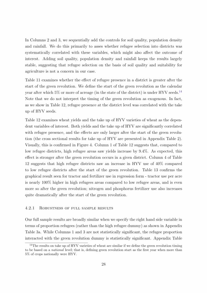
Table 11 examines whether the effect of refugee presence in a district is greater after the

start of the green revolution. We define the start of the green revolution as the calendar

year after which 5% or more of acreage (in the state of the district) is under HYV seeds.14

Note that we do not interpret the timing of the green revolution as exogenous. In fact,

as we show in Table 12, refugee presence at the district level was correlated with the take

up of HYV seeds.

Table 12 examines wheat yields and the take up of HYV varieties of wheat as the depen-

dent variables of interest. Both yields and the take up of HYV are significantly correlated

with refugee presence, and the effects are only larger after the start of the green revolu-

tion (the cross sectional results for take up of HYV are presented in Appendix Table 2).

Visually, this is confirmed in Figure 4. Column 1 of Table 12 suggests that, compared to

low refugee districts, high refugee areas saw yields increase by 9.4%. As expected, this

effect is stronger after the green revolution occurs in a given district. Column 4 of Table

12 suggests that high refugee districts saw an increase in HYV use of 40% compared

to low refugee districts after the start of the green revolution. Table 13 confirms the

graphical result seen for tractor and fertilizer use in regression form - tractor use per acre

is nearly 100% higher in high refugees areas compared to low refugee areas, and is even

more so after the green revolution; nitrogen and phosphorus fertilizer use also increases

quite dramatically after the start of the green revolution.

4.2.1 Robustness of full sample results

Our full sample results are broadly similar when we specify the right hand side variable in

terms of proportion refugees (rather than the high refugee dummy) as shown in Appendix

Table 3a. While Columns 1 and 3 are not statistically significant, the refugee proportion

interacted with the green revolution dummy is statistically significant. Appendix Table

14The results on take up of HYV varieties of wheat are similar if we define the green revolution timingto be based on a national level; that is, defining green revolution start as the first year when more than5% of crops nationally were HYV.

28

3b shows that these results are also robust to exclusion of mismatching data across the

overlapping years in the VDSA and IACD data sets. Appendix Table 4 restricts the

full sample results to the smaller set of districts that we use in the sub sample analysis

and the results are more or less consistent (although the results for wheat yields become

insignificant).

5 Mechanisms

Our empirical analysis has shown a positive relationship between the refugee presence who

arrived at partition and long-run agricultural development after the advent of the green

revolution in India. Why was it the case that agricultural development after the start

of the green revolution differed between areas with a greater or lesser extent of refugee

presence? And why did the difference persist for an extended period that stretched

beyond the intial phases of the green revolution? In this section we explore two possible

channels that provide answers to such questions.

The two channels we focus on are (1) human capital and (2) the land regime. Firstly,

the refugees who arrived in India differed in terms of their educational achievement and

occupational choices from both the natives of the districts in which they settled and the

evacuees who had left for Pakistan. Hence we argue for human capital as an important

pathway through which refugees shaped persistent differences in agricultural development

in the period after the start of the green revolution. Secondly, the post-independence

government of India in its efforts to resettle the refugees on agricultural land aggressively

implemented programs of land redistribution and consolidation in districts in which the

refugees settled in large numbers. Accordingly, we argue that land redistribution and

consolidation is another key channel through which high refugee areas were able to pull

ahead of low refugee areas in terms of their agricultural development once the green

revolution had started.

5.1 Refugees and Human Capital

5.1.1 Literacy

According to Bharadwaj, Khwaja, and Mian (2009) Indian districts that received refugees

at Partition experienced a net increase in their literacy rates. Simple correlations in

29

Appendix Table 5a show that refugee presence is indeed correlated with increased literacy

of Indian districts in the years after partition. The correlation coefficient between the

high refugee dummy and rural male literacy in 1961 is 0.1204 and is significant at the 10%

level. It increases in both magnitude and significance between 1961 and 1991. At least

part of the reason why refugees were associated with increases in literacy was because

they belonged to highly literate minority communities in the areas of Pakistan from where

they had emigrated. This is clear from Figure 5 that compares the pre-partition literacy

of the minority communities (i.e. hindus and sikhs) with the majority community (i.e.

muslims) in districts that became Pakistan. The stark difference between the literacy of

the various groups is quite revealing. The hindu and sikh minorities vastly out performed

the muslim majority in terms of literacy throughout the four pre-partition census years

of 1901, 1911, 1921 and 1931.

Figure 5: Hindu, Sikh and Muslim literacy prior to partition in districts that went to Pakistan.

Notes: The figure is based on the three colonial regions of Western Punjab, Sind and North

West Frontier Province, all of which became part of post-independence Pakistan

Official colonial documents also acknowledge the superior position held by the refugees in

terms of education in the Pakistani districts from which they came. For instance, literacy

was highest “among hindus and sikhs, among the non-christian population” of the Attock

district15. In the Lahore district the pre-eminence of the hindus in education was deemed

“remarkable” and the considerable progress that had been made in “education of sikh

males” recognized16. Interestingly, the 1929 Muzaffargarh district gazetteer went so far

as to suggest that “no special measures were necessary in the case of hindus and sikhs”

15Gazetteers, Punjab District. Gazetteer of the Attock District, 1907. Page 30416Gazetteers, Punjab District. Gazetteer of the Lahore District, 1893-94. Page 84

30

as they were “ready to take advantage of every opportunity” of providing education to

their children17. A more systematic record of statements contrasting the pre-partition

literacy rate of hindus and sikhs with those of the muslims in the districts that went to

Pakistan is given in Appendix Table A6.

Other sources, outside of the official colonial publications, also point to the contribution

the refugees had made to education. Raychaudhuri, Habib, and Kumar (1983) when dis-

cussing the aftermath of partition in Pakistan observe that the event led to the sudden

departure of teachers and instructors who mainly came from the hindu and sikh commu-

nities18. The First Five Year Plan of the Planning Commission of Pakistan acknowledges

the damage done to the educational sector by the “sudden departure of hindu teachers

and instructors” who had manned the staff of the technical institutions, schools, colleges

and universities in the country19. The Hartog (1929) committee report that reviewed

the growth of education in late colonial India notes that in the Western Punjab and the

North Western Frontier Province—both regions that later went to Pakistan—the hindus

and sikhs had done “good service to the cause of education by the maintenance of a large

number of schools and colleges”20.

Another reason why the refugees could have led to the persistent differences in literacy

documented in Appendix Table 5a is the inter-generational transmission of human capi-

tal. The correlation in human capital outcomes across generations is well documented in

the literature examining persistent human capital differences. Rocha, Ferraz, and Soares

(2017) find that the education of first generation immigrants into Brazil in the late nine-

teenth century, attracted through a state-sponsored open immigration policy, led to per-

sistent differences in literacy outcomes throughout the twentieth century. Wantchekon,

Klasnja, and Novta (2014) in their study on the US show that educated parents lead to

better living standards, a shift away from farming and greater political activism amongst

the future generations. Bleakley and Ferrie (2016) argue that it is through the cogni-

tive ability and social aptitudes of parents that the inter-generational transfer of human

capital takes place.

17Gazetteers, Punjab District. Gazetteer of the Muzaffargarh District, 1929. Page 29118Raychaudhuri, Tapan, Irfan Habib, and Dharma Kumar, eds. The Cambridge economic history of

India. Vol. 2. CUP Archive, 1983. Page 99819Planning Commission. Government of Pakistan. The First Five Year Plan 1955-60. (1957). Page 720Hartog, P.J., 1929. Interim Report of the Indian Statutory Commission: Review of Growth of

Education in British India by the Auxiliary Committee Appointed by the Commission . Vol. 3407. HMStationery Office. Page 246

31

We postulate that the persistent change in literacy outcomes brought by the refugees in

the districts in which they settled translated into the adoption of high yielding varieties

of seeds during the green revolution. Several papers show a positive relationship between

education and agricultural technology adoption. Rosenzweig (1978) finds that the prob-

ability of adopting high yield varieties of grain in the Indian Punjab is positively related

to farmer education and farm size. Sidhu (1976) in another study on the Indian Punjab

found that the education of farmers had a positive impact on both the crop yields and

gross sales revenue from the lands that were cultivated in the early stages of the Green

Revolution. Ram (1976) in yet another study on India shows that the contribution of

farm operators to production was positively related to their education. Schultz (1964),

Gerhart (1974) and Jamison, Lau, et al. (1982) all show similar relationships.

The argument usually put forward in such studies is that the adoption of agricultural

technology requires the ability to perceive, interpret, and respond to new events in the

context of risk, and that such ability is derived through human capital (Schultz, 1964).

The underlying hypothesis of such an argument is that education increases the ability of

farmers to “understand and evaluate the information on new products and processes”,

thereby incentivizing them to adopt new technologies (Feder, Just, and Zilberman, 1985).

Feder, Just, and Zilberman (1985) provide a comprehensive review of the broader liter-

ature connecting human capital to agricultural technology adoption. In our context, we

show using simple correlations in Appendix Table 5b, that literacy at the district level is

positively correlated to the take up of high yielding variety of seeds in the years subse-

quent to the start of the green revolution. The correlation coefficient between take up of

high yielding variety of all major crops and rural male literacy is 0.2691 in 1971, 0.0843

in 1981 and 0.2640 in 1991.

There is also some suggestive qualitative evidence that the higher literacy of the refugees

had already led to them engaging in superior farming practices even before partition. The

evidence relates to the minority hindu and sikh communities in those districts of colonial

India that later became Pakistan. For instance, the hindu Jats21 of Lyallpur district were

considered by the colonial administrators as being the “most useful class of peasants”22.

The hindu and sikh Jats of Sialkot district were deemed to be far superior cultivators

than their muslim counterparts23. The gazetteer of the Lahore district notes that the

21An agricultural caste of the Punjab22Gazetteers, Punjab District. Gazetteer of the Chenab Colony, 1904. Vol.A. Page 5123Gazetteers, Punjab District. Gazetteer of the Sialkot District, 1893-94. Page 75

32

hindu and sikh Jats were “good husbandsmen”24. The sikh Virakhs25 of the Montgomery

district were considered first-rate cultivators26. Most emphatically, the (1881) census of

the Punjab states that a substantial proportion of the sikh Jats belonging to the Lahore

and Gujranwala districts were “stalwart, sturdy yeomen of great independence, industry,

and agricultural skill” who collectively formed “perhaps the finest peasantry in India”27.

5.1.2 Money-Lending

Literacy is not the only dimension of human capital along which the refugees were differ-

ent from the native population. From the qualitative evidence we have gathered we know

that a significant number of the refugees were involved in small-scale money lending to

farmers for agricultural purposes in the districts from which they emigrated. They pro-

vided a “much needed source of credit for cultivation”(Raychaudhuri, Habib, and Kumar,

1983) for local farmers who would otherwise not have had access to formal credit mar-

kets. A substantial proportion amongst them belonged to the three great hindu and sikh

mercantile castes of India—Khatris, Aroras and Baniahs—that dominated commercial

activity. Figure 6 provides a snapshot of the advantage that the refugees had over the

native population in commercial occupations at the time of partition. It compares the

proportion of refugees engaged in commerce against the same proportion for the natives

based on actual data on both groups from the 1951 census of India. Again, the stark

contrast between the two groups in terms of their involvement in commerce is clearly

apparent.

As was the case with their educational superiority the higher concentration of the refugees

in money-lending in the areas where they came from was also noted in official publications

dating from the colonial period. The notes pertain to the hindu and sikh minority com-

munities in areas that later became Pakistan. For instance, the (1881) census of Punjab

states that the hindus and sikhs were mostly traders.28 Hindus from the Arora caste con-

trolled “almost the whole of the trade, moneylending, and banking” in the Muzaffargarh

district.29 The hindu Aroras were also considered as being the “chief moneylenders and

24Gazetteers, Punjab District. Gazetteer of the Lahore District, 1883-84. Page 6525An agricultural caste of the Punjab26Gazetteers, Punjab District. Gazetteer of the Montgomery District, 1898-99. Page 8627Report on the Census of the Panjab Taken on the 17th of February 1881. Page 22928Report on the Census of the Panjab Taken on the 17th of February 1881. Page 125-138.29Gazetteers, Punjab District. Gazetteer of the Muzaffargarh District, 1929. Page 78.

33

Figure 6: Refugees in the commercial sector

Notes: The black bar is the proportion of the displaced persons in 1951 that were previously

engaged in commerce. This data is given in Appendix II of Table IV of the 1951 census of

India. The grey bar is the proportion of the non-displaced persons (natives) that were previously

engaged in commerce. This data is also available in the 1951 census of India.

capitalists” and the “chief creditors of the agriculturists” in the Jhang district.30 The

hindus and sikhs from the Arora caste were identified as being the main moneylenders in

the Montgomery district31. In the Attock district “almost the whole trade and money-

lending business” was divided by the the three most numerically important hindu castes

amongst themselves32.

The higher concentration of the refugees in money-lending is likely to have had important

consequences for agricultural technology adoption. It is plausible that refugee presence

could have led to an expansion of credit to farmers that in turn led to faster adoption

of high yielding varieties during the green revolution. The argument that farmers who

are credit constrained find it difficult to adopt new agricultural technologies is well doc-

umented in the literature (Bhalla, 1979; Pitt and Sumodiningrat, 1991; Lipton, 1976).

Often, introducing a high yielding variety of seeds or purchasing a tractor requires having

access to loans because farmers simply do not have adequate savings that are required

to make such investments on their own. Access to credit then acts as a supplement to

savings that can be used to invest in agricultural technology. The provision of credit also

reduces the risks farmers face in their lives as it cushions them from extreme fluctuations

30 Gazetteers, Punjab District. Gazetteer of the Jhang District, 1883-84. (1884). Page 68.31Gazetteers, Punjab District. Gazetteer of the Montgomery District, 1883-84. (1884). Page 69-7032Gazetteers, Punjab District. Gazetteer of the Attock District, 1930. Page 115.

34

in agricultural output. The reduction in risk in turn makes them more likely to adopt

newer, more riskier, technologies. We, therefore, postulate that money-lending expertise

was another potential pathway through which the refugees could have influenced post

green revolution agricultural development in India.

5.2 Refugees and Land Reforms

5.2.1 Land Redistribution

As discussed in Section 1, the arrival of refugees was associated with land reforms that

were crucial to the adoption of high yielding varieties during the green revolution. The

first of these reforms was the substantial redistribution of land from large landholders to

small and medium sized owner-cultivators that took place amongst the refugee popula-

tion. One extreme example of redistribution occurred when one of the large landowners

amongst the refugees submitted a claim for 11,582 acres based on her previous land hold-

ings in Pakistan. In return, she received an allotment of only 835 acres, which represented

a 93 percent reduction in her previous land holdings (Kudaisya, 1995, p. 82). In addition

to dramatically reducing large landholdings the redistribution also increased small and

medium sized landholdings amongst the refugee population. It did so by allotting some of

the poorest refugee farmers small parcels of land, known as ‘plough units’, for cultivation

regardless of their holdings in Pakistan (Randhawa, 1954, p. 67).

The redistribution of land amongst the refugee population had important repercussions

for the long term agricultural development in the high-refugee districts. To begin with,

land redistribution increased the size of those landowning groups (i.e. small and medium

owner-cultivators) that were most likely to undertake the lumpy and/or risky investments

required for improving agricultural productivity.33 According to Kudaisya (1995) it was

the superior risk taking ability of the refugee farmers that “enabled them to make signifi-

cant changes in their methods of irrigation and farming” that were required for adopting

HYVs during the green revolution.

The redistribution also affected farming incentives within the refugee community in a

way that was beneficial to agricultural development. By forcing large landowners to take

33The link between small and medium sized owner cultivators and intensity of agricultural technologyadoption is well established in the literature. For example Muthiah (1971), Schluter (1971) and Sharma(1973) all find that the proportion of acreage devoted to high yielding varieties on small and mediumsized farms in India is higher than the corresponding number for large farms.

35

up cultivation themselves rather than live as absentee landlords and by giving land to

landless labourers it increased the incidence of owner-cultivation amongst the refugee

population. Since owner-cultivators have superior incentives relative to tenant farmers

and landless labourers,34 the redistribution of land contributed to agricultural technology

adoption and productivity through through the channel of incentives. Indeed, Kudaisya

(1995) credits the process through which evacuee land was redistributed to refugees with

creating a system of peasant-proprietorships through which agriculturists in general were

encouraged to ‘work hard and stand on their own feet’.

5.2.2 Land Consolidation

Another important change in the land regime associated with the arrival of refugees was

the consolidation of fragmented land. The need to consolidate fragmented land for im-

proving agricultural productivity had been officially recognised since the enactment of the

Punjab Consolidation Act in 1936 during the colonial period. However, progress in the

field of land consolidation had been slow up until Partition. The large number of prop-

erty transfers involved in redistributing evacuee land to refugees provided the required

impetus behind accelerating the process of land consolidation shortly after Partition.

Consequently, efforts towards land consolidation picked up pace through the enactment

of the East Punjab Consolidation and Fragmentation Act in 1948. The legislation im-

posed ‘restrictions on the creation of fragments as a preventive measure of consolidation’

(Sarkar, 1989, p. 84). For instance, one of the clauses of the Act prohibited any trans-

fer or partitioning of land that could result in the creation of a fragment (Sarkar, 1989,

p. 84). Another clause barred the practice of fragmenting undivided agricultural land for

distribution amongst inheritors. In addition to the Act of 1948 a series of further laws

were passed for promoting the consolidation of landholdings (Gill, 1989, p. 80). A sep-

arate department was even opened by the East Punjab government for the sole purpose

of enforcing land consolidation (Gill, 1989, p. 80). As a result of legislation and other

proactive measures taken by the government, the size of consolidated land holdings went

up from 700,000 acres in 1948 to over 22.084 million acres in 1966 in East Punjab as a

whole (Kudaisya, 1995, p. 83). Most of consolidation took place in districts where the

34The argument that cultivating other people’s land rather than your own leads to incentive problemsthat reduce investment and productivity is well established in the literature (See Banerjee and Iyer (2005)for reference).

36

problem of land fragmentation had become especially acute as a result of refugees settling

in large numbers.

The increase in consolidated land in high refugee districts could have influenced the

adoption of HYVs during the Green Revolution in several ways. First, large areas of

wasteland, such as embankments and field boundaries, under the previous fragmented

land regime were brought under cultivation through consolidation. The increase in plot

size that accompanied such consolidation could have led to farmers being more willing

to experiment with planting the new, more risky, HYVs on a fraction of their cultivated

land. Second, farmers with consolidated landholdings could have found it economically

viable to sink tube-wells in their farms to gain access to sub-soil water for cultivation. It

was largely through land consolidation that the number of tube-wells in East Punjab rose

from close to zero in 1950 to 570,000 in 1978 (Kudaisya, 1995, p. 83). The increased access

to sub-soil water that farmers were able to secure through consolidation was crucial to the

adoption of high yielding varieties that depended on the timely and controlled provision

of water. Finally, land consolidation could also have led to improved access to canal

irrigation since supplying canal-irrigated water to tiny scattered plots under the previous

fragmented land regime had been practically impossible (Kudaisya, 1995, p. 84). Just as

was the case with sub-soil water, the access to canal irrigated water proved vital to the

adoption of high yielding varieties during the green revolution.

6 Conclusion

In this study, we examine the impact of the partition of India on the take up of agricultural

technology and agricultural productivity post-partition. Using refugee presence as a proxy

for the intensity of the impact of partition, we find that areas with more refugees have

higher average yields, are more likely to take up High Yielding Varieties (HYV) of seeds,

and are more likely to use agricultural technologies within the first 60 years after partition

in India. In particular, we show that more affected districts diverge from the less affected

districts after the start of the Green Revolution in the late 1960s. We further show,

using pre-partition agricultural data, that the effects are not solely explained by selective

refugee movement into districts with a higher potential for agricultural development.

While limited in our ability to explore empirically the potential pathways through which

the partition impacted long run agricultural development, we nonetheless argue that

the greater levels of education of the refugees and their higher concentration in money-

37

lending contributed to agricultural development. Additionally, we also provide qualitative

evidence for the role of land reforms soon after partition, particularly in areas with

refugees, as a factor in explaining higher agricultural productivity.

While our study makes progress on an important question about the legacy of India’s

partition, there are several aspects that we hope future work can address. Prime among

these is the effects of the partition in the long run on the Pakistani side. While data

limitations prevent us from doing a similar analysis for agriculture, perhaps other relevant

outcomes such as literacy and urbanization could be analyzed. Future work on land

reforms after the partition would lend fascinating insights into why places affected by

refugee settlement evolved differently, as would work on other mechanisms (political,

social capital, religious homogeneity) that may explain the patterns seen in this paper.

38

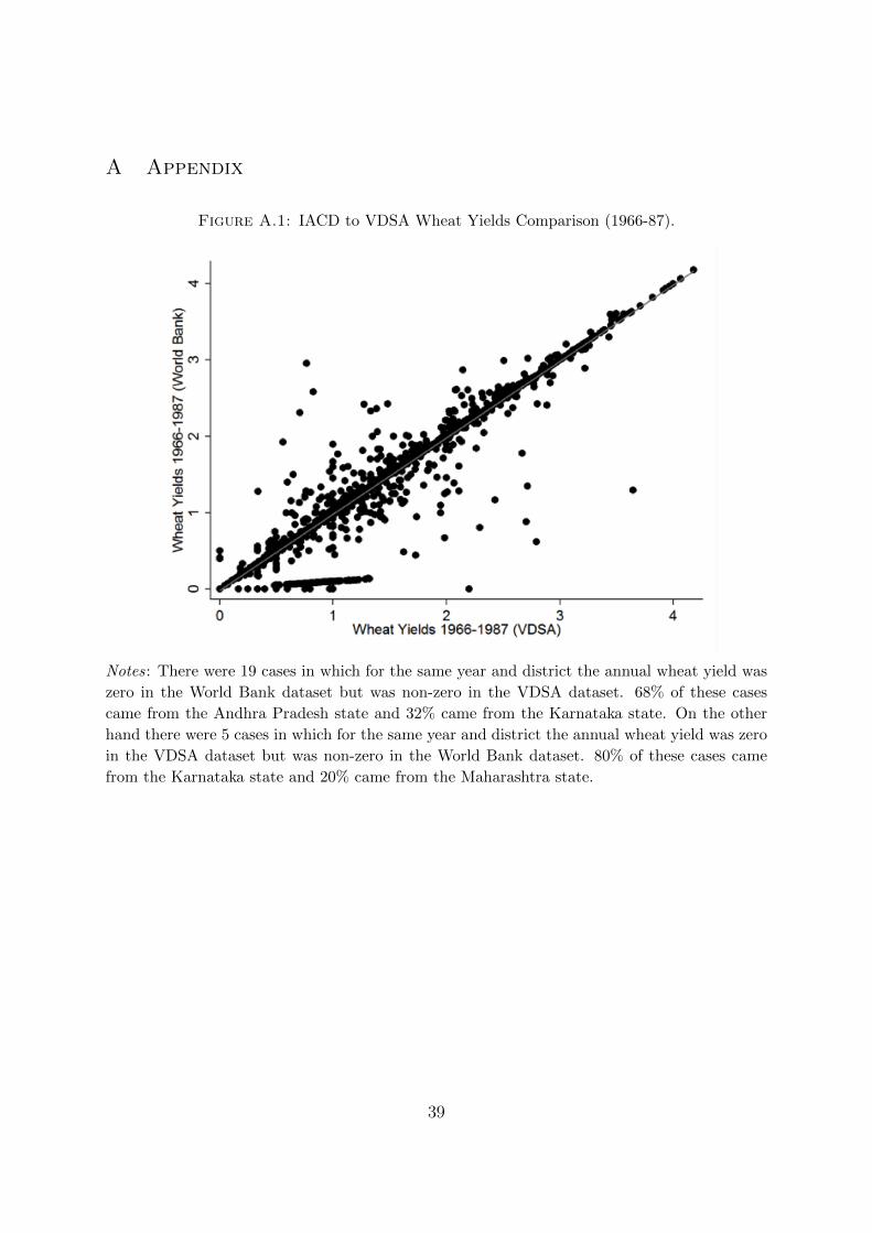
A Appendix

Figure A.1: IACD to VDSA Wheat Yields Comparison (1966-87).

Notes: There were 19 cases in which for the same year and district the annual wheat yield was

zero in the World Bank dataset but was non-zero in the VDSA dataset. 68% of these cases

came from the Andhra Pradesh state and 32% came from the Karnataka state. On the other

hand there were 5 cases in which for the same year and district the annual wheat yield was zero

in the VDSA dataset but was non-zero in the World Bank dataset. 80% of these cases came

from the Karnataka state and 20% came from the Maharashtra state.

39

Figure A.2: IACD to VDSA Wheat HYV Take Up Comparison (1966-87).

Notes: There were 22 cases in which for the same year and district the annual fraction of HYV

of wheat was zero in the World Bank dataset but was non-zero in the VDSA dataset. 82%

of these cases came from the Maharashtra state, 9% came from the Gujarat state, 4.5% from

Rajasthan state and 4.5% from Tamil Nadu state. On the other hand there were 475 cases in

which for the same year and district the annual fraction of HYV of wheat was zero in the VDSA

dataset but was non-zero in the World Bank dataset. 98.3% of these cases came from the Uttar

Pradesh state, 0.9% came from the Andhra Pradesh state, 0.2% came from the Gujarat state,

0.4% came from the Madhya Pradesh state and 0.2% came from the Orissa state.

40

B Appendix

West Bengal Refugee Resettlement: Rather than coming in one big rush around

the time of Partition, as was the case with the East Punjabi refugees, the West Bengali

refugees instead came in waves over a prolonged period. The prolonged nature of the

migration from East Pakistan to West Bengal was due to the gradual deterioration in the

security situation of the minorities in East Pakistan after Partition. Initially, the hindu

minorities felt safe enough to remain behind in East Pakistan. However, after 1950 when

tensions between the muslim and hindu communities began to rise, many of the hindus

who had originally decided to remain behind in East Pakistan at the time of Partition

decided to leave for West Bengal in India.

Unlike its East Punjabi counterpart, the government of West Bengal failed to resettle

refugees on agricultural land. Part of the reason behind this failure was the deliberate

policy of both the Indian and Pakistani governments to avoid a population exchange

between West Bengal and East Pakistan. A clear reflection of the policy was the Nehru-

Liaqat pact of 1950. The Pact aimed at creating a sense of security amongst minorities

in both East and West Bengal to avoid population exchange across the Partition border

(Kudaisya, 1995, p. 87). In accordance with its policy of avoiding population exchange,

the West Bengal government did not make any detailed plans regarding the distribution

of land to refugees. Consequently, many of the refugees ended up becoming landless and

congregated in areas around Calcutta city, forming a vast urban underclass (Kudaisya,

1995, p. 90). Another factor behind the West Bengal government’s failure to resettle

refugees was the amount of evacuee land available after Partition. The number of Muslim

evacuees who left for East Pakistan was far less than the number of hindu refugees who

replaced them in West Bengal (Kudaisya, 1995, p. 89). Moreover, the Muslim evacuees

who left for East Pakistan were mostly either landless peasants or small-scale farmers

with meagre land holdings. Such a situation meant that the evacuee land available for

resettling refugees was insufficient.

Up until 1950, most of the refugees who arrived in West Bengal “came from the middle

classes and relied on their own resources to begin life afresh” in their new homeland

(Kudaisya, 1995, p. 89). However, when fresh riots broke out in East Bengal in early

1950, many hindu agriculturists were forced to migrate to West Bengal. Such a change

in the economic profile of the incoming refugees caused a fundamental shift in the nature

of the rehabilitation problem faced by the West Bengal government. The post-1950

41

refugees came with “few possessions, capital or skills” and urgently sought resettlement

on agricultural land (Kudaisya, 1995, p. 87). The government, however, was slow in

responding to the refugee resettlement problem. As late as 1958, almost eleven years

after Partition, the West Bengal government had “been able to acquire only 61,000 acres

of agricultural land for redistribution among the refugees, which was hardly adequate

considering the numbers involved” (Kudaisya, 1995, p. 89).

Eventually, the official policy on refugees shifted from ignoring the land resettlement

needs of the refugees to actively resettling refugees on agricultural land. The policy shift

manifested itself in the form of the Dandakaranya scheme. The scheme represented the

West Bengal government’s attempt at finding ‘a long-term solution for the resettlement

of the East Bengali refugees’ (Kudaisya, 1995, p. 91). According to the scheme, refugees

were allotted land in the Dandakaranya region that comprised the districts of Bastar

in Madhya Pradesh State and Kalahandi and Koraput in Orissa State. Initially, the

scheme looked promising with around 12,000 refugee families being allotted land in the

Dandakaranya region by 1967. However, a major drawback of the scheme was that the

agricultural conditions in Dandakaranya were unsuitable for paddy – a crop the refugees

specialized in cultivating. Dandakaranya was a forested plateau where the soil was hard,

red, and porous and, as a result, the potential for surface irrigation was limited (Kudaisya,

1995, p. 91). All these factors severely limit the potential for paddy cultivation. Once

the refugees realized that the land they had been allotted was severely limited in terms

of its potential for large-scale paddy cultivation, they abandoned their holdings and left.

Between 1972 and 1978, some 10,923 refugee families deserted their land holdings in the

region. The Dandakaranya scheme had completely failed by the late 1970s.

The failure of the Dandakaranya scheme and the lack of state support for resettlement

led to some refugees creating their own settlements by clearing forests and colonising

agricultural lands in regions of Eastern India like the Sunderbans, Assam valley, and

Tripura. Despite such independent efforts, the bulk of the refugee community remained

landless throughout the post-partition period (Kudaisya, 1995, p. 86).

42

References

Acemoglu, D., T. A. Hassan, and J. A. Robinson (2011): “Social Structure and

Development: A Legacy of the Holocaust in Russia,” The Quarterly journal of eco-

nomics, 126(2), 895–946.

Acemoglu, D., S. Johnson, and J. A. Robinson (2002): “Reversal of Fortune:

Geography and Institutions in the Making of the Modern World Income Distribution,”

The Quarterly Journal of Economics, 117(4), 1231–1294.

Banerjee, A., and L. Iyer (2005): “History, Institutions, and Economic Performance:

The Legacy of Colonial Land Tenure Systems in India,” The American Economic Re-

view, 95(4), 1190–1213.

Bhalla, S. S. (1979): “Farm and Technical Change in Indian Agriculture,” .

Bharadwaj, P., and J. Fenske (2012): “Partition, migration, and jute cultivation in

India,” Journal of Development Studies, p. 1.

Bharadwaj, P., A. Khwaja, and A. Mian (2008): “The big march: migratory flows

after the partition of India,” Economic and Political Weekly, pp. 39–49.

Bharadwaj, P., A. I. Khwaja, and A. R. Mian (2009): “The partition of India:

demographic consequences,” .

Bleakley, H., and J. Ferrie (2016): “Shocking behavior: Random wealth in an-

tebellum Georgia and human capital across generations,” The quarterly journal of

economics, 131(3), 1455–1495.

Byerlee, D., and P. Moya (1993): Impacts of international wheat breeding research

in the developing world, 1966-1990. CIMMYT.

Chakravarti, A. (1973): “Green revolution in India,” Annals of the Association of

American Geographers, 63(3), 319–330.

Chaney, E., and R. Hornbeck (2015): “Economic Dynamics in the Malthusian Era:

Evidence from the 1609 Spanish Expulsion of the Moriscos,” The Economic Journal.

Chaudhary, L., and J. Rubin (2011): “Reading, writing, and religion: Institutions

and human capital formation,” Journal of Comparative Economics, 39(1), 17–33.

43

Christopher, A. J. (2011): “Secession and South Sudan: an African precedent for the

future?,” South African Geographical Journal, 93(2), 125–132.

D’Agostino, A. (2017): “Technical Change and Gender Wage Inequality: Long-Run

Effects of India?s Green Revolution,” Working Paper.

Dell, M. (2010): “The persistent effects of Peru’s mining mita,” Econometrica, 78(6),

1863–1903.

Dippel, C. (2014): “Forced coexistence and economic development: Evidence from

native american reservations,” Econometrica, 82(6), 2131–2165.

Donaldson, D. (2010): “Railroads of the Raj: Estimating the impact of transportation

infrastructure,” Discussion paper, National Bureau of Economic Research.

Evenson, R. E., and D. Gollin (2003): “Assessing the impact of the Green Revolu-

tion, 1960 to 2000,” Science, 300(5620), 758–762.

Feder, G., R. E. Just, and D. Zilberman (1985): “Adoption of agricultural innova-

tions in developing countries: A survey,” Economic development and cultural change,

pp. 255–298.

Foster, A. D., and M. R. Rosenzweig (1996): “Technical change and human-capital

returns and investments: evidence from the green revolution,” The American economic

review, pp. 931–953.

Gerhart, J. D. (1974): “The diffusion of hybrid maize in western Kenya,” PhD Dis-

sertation, Princeton University.

Gill, S. S. (1989): “Changing land relations in Punjab and implications for land re-

forms,” Economic and Political Weekly, pp. A79–A85.

Gollin, D., C. W. Hansen, and A. M. Wingender (2016): “Two Blades of Grass:

The Impact of the Green Revolution,” Centre for Economic Policy Research Discussion

Paper DP11611.

Hartog, P. J. (1929): ... Interim Report of the Indian Statutory Commission:(Review

of Growth of Education in British India by the Auxiliary Committee Appointed by the

Commission)..., vol. 3407. HM Stationery Office.

Heston, A. W. (1973): “Official Yields Per Acre in India, 1886-1947: Some Questions

of Interpretation,” Indian Economic & Social History Review, 10(4), 303–332.

44

Hornbeck, R., and S. Naidu (2014): “When the levee breaks: black migration

and economic development in the American South,” The American Economic Review,

104(3), 963–990.

Iyer, L. (2010): “Direct versus indirect colonial rule in India: Long-term consequences,”

The Review of Economics and Statistics, 92(4), 693–713.

Jamison, D. T., L. J. Lau, et al. (1982): Farmer education and farm efficiency.

Johns Hopkins University Press.

Jha, S. (2013): “Trade, Institutions, and Ethnic Tolerance: Evidence from South Asia,”

American Political Science Review, 107(04), 806–832.

Jha, S., and S. Wilkinson (2012): “Does combat experience foster organizational

skill? Evidence from ethnic cleansing during the partition of South Asia,” American

Political Science Review, 106(04), 883–907.

Khan, Y. (2017): The great partition: The making of India and Pakistan. Yale University

Press.

Kliot, N., and Y. Mansfield (1997): “The political landscape of partition: the case

of Cyprus,” Political geography, 16(6), 495–521.

Kudaisya, G. (1995): “The demographic upheaval of partition: Refugees and agricul-

tural resettlement in India, 1947–67,” South Asia: Journal of South Asian Studies,

18(s1), 73–94.

Kumar, R. (2004): “Settling Partition Hostilities: Lessons Learned, Options Ahead,”

The Fate of the Nation-state, p. 247.

Lipton, M. (1976): “Agricultural finance and rural credit in poor countries,” World

Development, 4(7), 543–553.

Mohan, R., and R. E. Evenson (1975): “The intensive agricultural districts pro-

gramme in India: A new evaluation,” The Journal of Development Studies, 11(3),

135–154.

Munshi, K. (2004): “Social learning in a heterogeneous population: technology diffusion

in the Indian Green Revolution,” Journal of development Economics, 73(1), 185–213.

Muthiah, C. (1971): “The Green Revolution-Participation by Small and Large Farm-

ers,” Indian Journal of Agricultural Economics, 26(1), 53.

45

NCAI-I (1976): “Report of the National Commission on Agriculture, 1976,” .

NCAI-V (1976): “Report of the National Commission on Agriculture, 1976,” .

Nunn, N. (2008): “The Long-Term Effects of Africa’s Slave Trades,” The Quarterly

Journal of Economics, 123(1), 139–176.

(2009): “The importance of history for economic development,” Discussion

paper, National Bureau of Economic Research.

Peters, M. (2017): “Refugees and Local Agglomeration: Evidence from Germany’s

Post-War Population Expulsions,” Yale University Working Paper.

Pitt, M. M., and G. Sumodiningrat (1991): “Risk, schooling and the choice of seed

technology in developing countries: a meta-profit function approach,” International

Economic Review, pp. 457–473.

Ram, R. (1976): “Education as a quasi factor of production: the case of India’s agricul-

ture,” Ph.D. thesis, University of Chicago, Department of Education.

Randhawa, M. S. (1954): Out of the ashes: An account of the rehabilitation of refugees

from West Pakistan in rural areas of East Punjab. Public Relations Dept., Punjab.

Raychaudhuri, T., I. Habib, and D. Kumar (1983): The Cambridge Economic

History of India: Volume 2, C. 1751-c. 1970, vol. 2. CUP Archive.

Rocha, R., C. Ferraz, and R. R. Soares (2017): “Human capital persistence and

development,” American Economic Journal: Applied Economics, 9(4), 105–36.

Rosenzweig, M. R. (1978): “Schooling, allocative ability and the green revolution,”

Paper presented at the meetings of the Eastern Economic Association, Washington,

D.C.

Rud, J. P. (2012): “Electricity provision and industrial development: Evidence from

India,” Journal of development Economics, 97(2), 352–367.

Sarkar, B. (1989): Land Reforms in India, Theory and Practice: A Study of Legal

Aspects of Land Reforms Measures in West Bengal. APH Publishing.

Schluter, M. (1971): Differential Rates of Adoption of the New Seed Varieties in

India: The Problem of the Small Farm. Department of Agricultural Economics, Cornell

University.

46

Schultz, T. W. (1964): Transforming Traditional Agriculture. Yale University Press,

New Haven, CT.

Sharma, A. (1973): “Influence of certain economic and technological factors on the

distribution of cropped area under various crops in the Ludhiana district,” Journal of

Research (Punjab Agricultural University), 10, 243–49.

Sidhu, S. S. (1976): “The Productive Value of Education in Agricultural Development,”

Discussion paper, University of Minnesota, Department of Applied Economics.

Singh, T. (1952): Land Resettlement Manual for Displaced Persons in Punjab & Pepsu.

Controller of Printing & Stationary.

Visaria, P. M. (1969): “Migration between India and Pakistan, 1951–61,” Demography,

6(3), 323–334.

Wantchekon, L., M. Klasnja, and N. Novta (2014): “Education and human cap-

ital externalities: evidence from colonial Benin,” The Quarterly Journal of Economics,

130(2), 703–757.

Yong, T. T., and G. Kudaisya (2000): The Aftermath of Partition in South Asia.

London, Routledge.

47

Variable Mean MedianStandard

Deviation

Number of

Observations

Annual Wheat Yields (1957-2009) (tons per hectare) 1.489 1.292 0.893 12763

Annual Take-Up of HYVs of Wheat (1957-2009) (proportion) 0.070 0.005 0.128 11573

Annual Revenue per hectare based on 1960 prices (rupees per hectare) 493.391 386.945 356.939 11500

Annual consumption of Nitrogen Fertilizer (tons) 40.241 16.262 118.801 13001

Annual consumption of Phosphorus Fertilizer (tons) 15.812 5.906 50.427 13001

Annual consumption of Potassium Fertilizer (tons) 10.257 1.258 99.389 13001

Annual number of tractors per 1000 hectares (1957-1987) 1.811 0.395 4.896 8370

Log Refugees (1951) 7.443 7.549 2.576 270

Log of Population (1951) 13.792 13.846 0.639 270

High Refugee Dummy (1951) 0.485 … … 270

Proportion Refugees (1951) 0.021 0.002 0.055 269

Annual Rainfall (1957-2009) (millimeters) 1039.807 945.000 573.994 13971

Population Desnity (1961) 1.789 1.251 2.117 270

Table 1A. Summary Statistics

Notes: Data on annual rainfall does not change between 1957 and 1965. This is because the Indian Agriculture and Climate Dataset from

which the data between 1957 and 1965 is taken only provides estimated average rainfall for each district for each month across all the

years between 1957 and 1987. Data for the annual number of tractors from 1988 to 2009 does not exist. This because the Village

Dynamics in South Asia Dataset from which the data from between 1957 to 2009 was supposed to be taken does not include information

on tractors.

Variable Actual Mean Median Std. Dev Observations ActualProportion of

Full SampleMean Median Std. Dev Observations

Proportion of

Full Sample

Number of Refugees (1951) 5862319 … … … 265 3329178 57% … … … 67 25%

Population (1951) 302980160 … … … 265 94666560 31% … … … 67 25%

Annual Wheat Yields (lbs per acre) … 1328.77 1152.56 796.56 12763 … … 1341.08 1106.13 838.29 3870 30%

Annual Rice Yields (lbs per acre) … 1213.27 1009.41 736.97 13396 … … 894.47 378.50 1468.52 3427 26%

Annual Maize Yields (lbs per acre) … 1190.27 973.29 817.38 12758 … … 1175.99 1049.76 656.69 3508 27%

Annual Jowar Yields (lbs per acre) … 631.79 590.52 388.95 11840 … … 652.58 632.14 386.15 2950 25%

Annual Bajra Yields (lbs per acre) … 653.52 575.19 418.15 8514 … … 658.07 580.00 416.91 2395 28%

Annual Rainfall (millimeters) … 1040.65 946.00 574.73 13926 … … 1013.19 949.30 437.26 3470 25%

Altitude (meters) … 353.38 357.00 140.20 13878 … … 424.72 396.00 212.03 3939 28%

Latitude (degrees) … 22.78 23.45 4.85 13878 … … 24.61 24.96 3.92 3939 28%

Longitude (degrees) … 78.82 78.11 4.36 13878 … … 79.43 78.43 4.57 3939 28%

Table 1B: Summary Statistics comparison between full and restricted sample

Full Sample (1957-2009) Restricted Sample (1911-2009)

Notes: The unit of observation is a district and year. Data on annual rainfall does not change between 1957 and 1965 and is only available from 1957 onwards. Restricted sample is the

sample of 67 districts for which data is consistently available from 1911 to 2009. Full sample is the sample of districts in the dataset from 1957 onwards.

(1) (2) (3) (4) (5) (6) (7) (8)

Post Partition X Var 32.3 32.24 150.1** 150.0**

(21.82) (23.33) (60.99) (65.21)

Post GR X Var 53.10** 196.3***

(25.69) (72.67)

1957-1967 X Var -6.926 2.094

(15.78) (44.99)

1967-1977 X Var 8.937 67.05

(22.20) (57.10)

1977-1987 X Var 51.11 183.5**

(31.00) (81.00)

1987-1997 X Var 63.16* 251.4***

(33.19) (93.12)

1997-2009 X Var 42.26 224.1**

(34.76) (106.0)

Mean outcome 1351 1351 1351 1351 1351 1351 1351 1351

Observations 3785 3785 3785 3785 3785 3785 3785 3785

R-squared 0.893 0.925 0.926 0.926 0.914 0.946 0.948 0.927

Controls:

Main effects Yes Yes Yes Yes Yes Yes Yes Yes

State FE Yes No No No Yes No No No

State polynomial trends Yes No No No Yes No No No

State X Year FE No Yes Yes Yes No Yes Yes Yes

Geographic controls Yes Yes Yes Yes Yes Yes Yes Yes

Table 2: Wheat Yields and Refugees

Log Refugees High Refugee Dummy

Robust standard errors in parentheses, clustered at the district level

The unit for yields is lbs per acre. Geographic controls include 21 dummies for district soil type, latitude, longitude and altitude.

*** p<0.01, ** p<0.05, * p<0.1

(1) (2) (3) (4) (5) (6) (7) (8)

Sugarcane Maize Sorghum Pearl millets Other millets Chickpea Rapeseed Linseed

Post Partition X High Refugee Dummy 360.8** 48.19 -93.74 20.05 -122.2 53.25 170.9 1.538

(164.4) (121.6) (85.68) (63.38) (103.7) (50.65) (104.0) (18.34)

Mean outcome 4446 1182 654 661 664 646 561 329

Observations 3,656 3,441 2,918 2,367 1,130 3,108 2,948 1,786

R-squared 0.530 0.492 0.329 0.418 0.188 0.055 0.524 0.480

Controls:

Main effects Yes Yes Yes Yes Yes Yes Yes Yes

State FE Yes Yes Yes Yes Yes Yes Yes Yes

State linear trends Yes Yes Yes Yes Yes Yes Yes Yes

Geographic controls Yes Yes Yes Yes Yes Yes Yes Yes

*** p<0.01, ** p<0.05, * p<0.1

The unit for yields is lbs per acre. Geographic controls include 21 dummies for district soil type, latitude, longitude and altitude.

Robust standard errors in parentheses, clustered at the district level

Table 3: Refugee presence and other crops

(1) (2) (3) (4) (5) (6)

Post Partition X Var 2.164 -0.717 62.80

(7.533) (22.55) (57.69)

Post GR X Var 8.940* 31.37** 30.93**

(5.239) (14.16) (13.75)

Mean outcome 1351 1351 1351 1351 1351 1351

Observations 3,785 3,785 3,785 3,785 3,785 3,785

R-squared 0.885 0.878 0.884 0.878 0.886 0.879

Controls:

Main effects Yes Yes Yes Yes Yes Yes

All double interactions N/A N/A No No Yes Yes

State FE Yes Yes Yes Yes Yes Yes

State polynomial trends Yes Yes Yes Yes Yes Yes

Geographic controls Yes Yes Yes Yes Yes Yes

Table 4: Wheat Yields and Other proxies

Robust standard errors in parentheses, clustered at the district level

*** p<0.01, ** p<0.05, * p<0.1

Proportion Muslim in 1931Proportion Muslim in 1931 X Inverse Distance to the

border

The unit for yields is lbs per acre. Geographic controls include 21 dummies for district soil type, latitude, longitude and

altitude.

(1) (2) (3) (4)

Post Partition X Var 154.1** 154.0**

(59.84) (63.99)

Post GR X Var 197.0***

(70.74)

1957-1967 X Var -0.578

(45.52)

1967-1977 X Var 57.81

(56.42)

1977-1987 X Var 184.1**

(77.11)

1987-1997 X Var 236.7**

(91.03)

1997-2009 X Var 200.3*

(102.6)

Mean outcome 1351 1351 1351 1351

Observations 3,785 3,785 3,785 3,785

R-squared 0.896 0.928 0.930 0.929

Main effects Yes Yes Yes Yes

State FE Yes No No No

State polynomial trends Yes No No No

State X Year FE No Yes Yes Yes

Aquifer depth Yes Yes Yes Yes

Aquifer depth X Post Partition Yes Yes No No

Aquifer depth X Post GR No No Yes No

Aquifer depth X Decade FE No No No Yes

Geographic controls Yes Yes Yes Yes

*** p<0.01, ** p<0.05, * p<0.1

Geographic controls include 21 dummies for district soil type, latitude, longitude and altitude.

Table 5: Wheat Yields and Refugees accounting for soil conditions and aquifer depth after partition

High Refugee Dummy

Robust standard errors in parentheses, clustered at the district level

(1) (2) (3) (4) (5) (6) (7) (8) (9) (10) (11)

Area sown with

canal irrigation in

1938

Hospitals per

capita in 1961

Schools per

capita in 1961

Post offices

per capita in

1961

Banks per

capita in 1961

Length of

roads in

district in 1966

Total

geographic

area of district

Growth in

literate

population

1911-1921

Aquifer

Depth 1

Aquifer

Depth 2

Aquifer

Depth 3

High Refugee Dummy -0.0114 3.17e-06 -0.0002** -1.34e-05 -5.47e-07 534.3* -50.81 0.0319 -0.0305 0.143 0.0129

(0.180) (4.64e-06) (5.80e-05) (3.10e-05) (1.31e-06) (308.3) (93.50) (0.0689) (0.0941) (0.100) (0.0408)

Proportion of Muslims in 1931 -1.050 -2.45e-05 -1.29e-05 2.28e-05 6.44e-06 1,896 -9.889 -0.00676 0.00380 -0.784*** 0.851***

(0.803) (2.03e-05) (0.000124) (2.52e-05) (5.24e-06) (1,234) (130.1) (0.119) (0.0631) (0.287) (0.267)

Inverse distance to the border 10.24* -9.08e-06 -0.000615 1.36e-05 -1.61e-05 2,655 661.0 -0.446 -1.694 -2.906 3.026

(5.930) (0.000165) (0.000568) (0.000357) (3.34e-05) (3,438) (788.3) (0.863) (1.271) (2.453) (1.937)

Prop Muslim X Inverse distance

to the border-1.218 -6.42e-05 -0.000228 0.000128 3.47e-05 6,523 124.6 -0.0596 -0.382 -3.427*** 3.799***

(3.159) (0.000124) (0.000431) (0.000184) (2.35e-05) (3,947) (446.3) (0.434) (0.363) (0.950) (0.808)

Controls Yes Yes Yes Yes Yes Yes Yes Yes Yes Yes Yes

Observations 197 61 62 45 60 65 67 67 67 67 67

Robust standard errors in parentheses

*** p<0.01, ** p<0.05, * p<0.1

Table 6: Proxies and pre partition/green revolution infrastructure

Controls: State fixed effects and district area in all regressions (except column 8). Also included are controls for district level soil characteristics, latitude, longitude and altitude.

(1) (2) (3) (4) (5) (6) (7) (8)

Post Partition X Var 28.27 28.21 133.5** 133.4**

(19.98) (21.46) (59.25) (63.65)

Post GR X Var 48.31** 186.4**

(24.09) (70.95)

1957-1967 X Var -7.457 -8.465

(15.60) (45.00)

1967-1977 X Var 5.300 45.79

(20.75) (56.44)

1977-1987 X Var 44.17 148.4*

(26.55) (75.15)

1987-1997 X Var 59.50* 239.3**

(31.91) (93.88)

1997-2009 X Var 37.18 217.2**

(33.44) (103.7)

Mean outcome 1307 1307 1307 1307 1307 1307 1307 1307

Observations 3,557 3,557 3,557 3,557 3,557 3,557 3,557 3,557

R-squared 0.892 0.927 0.928 0.928 0.891 0.926 0.928 0.928

Controls:

Main effects Yes Yes Yes Yes Yes Yes Yes Yes

State FE Yes No No No Yes No No No

State polynomial trends Yes No No No Yes No No No

State X Year FE No Yes Yes Yes No Yes Yes Yes

Geographic controls Yes Yes Yes Yes Yes Yes Yes Yes

Table 7: Wheat Yields and Refugees - Excluding IADP districts

Log Refugees High Refugee Dummy

Robust standard errors in parentheses, clustered at the district level

*** p<0.01, ** p<0.05, * p<0.1

The unit for yields is lbs per acre. Geographic controls include 21 dummies for district soil type, latitude, longitude and altitude.

(1) (2)

Post Partition X High Refugee Dummy 120.8** 120.8*

(58.01) (62.14)

Banerjee-Iyer District X Post 188.2*** 188.2***

(65.44) (70.11)

Mean outcome 1361 1361

Observations 3,690 3,690

R-squared 0.896 0.928

Controls:

Main effects Yes Yes

State FE Yes No

State polynomial trends Yes No

State X Year FE No Yes

Geographic controls Yes Yes

*** p<0.01, ** p<0.05, * p<0.1

Table 8: Wheat Yields and Refugees - accounting for Banerjee & Iyer (2005) districts

Wheat Yields

Robust standard errors in parentheses, clustered at the district level. Tables notes are the same as in Table 2,

with the addition of districts level data from Banerjee and Iyer (2005), which classify districts based on various

types of colonial tax regimes.

(1) (2) (3) (4) (5) (6) (7) (8)

Post Partition X Var 109.6** 109.6** 359.6*** 359.6***

(40.30) (42.76) (110.5) (117.2)

Post GR X Var 111.2** 315.8**

(43.57) (126.7)

1957-1967 X Var 21.59 120.7

(31.08) (77.25)

1967-1977 X Var 61.55 230.4**

(40.75) (99.39)

1977-1987 X Var 119.9** 379.1**

(53.19) (138.0)

1987-1997 X Var 181.1*** 556.0***

(55.10) (153.6)

1997-2009 X Var 151.5** 476.6**

(61.57) (182.5)

Mean outcome 1875 1875 1875 1875 1875 1875 1875 1875

Observations 1,421 1,421 1,421 1,421 1,421 1,421 1,421 1,421

R-squared 0.926 0.950 0.952 0.954 0.927 0.951 0.953 0.955

Controls:

Main effects Yes Yes Yes Yes Yes Yes Yes Yes

State FE Yes No No No Yes No No No

State polynomial trends Yes No No No Yes No No No

State X Year FE No Yes Yes Yes No Yes Yes Yes

Geographic controls Yes Yes Yes Yes Yes Yes Yes Yes

The sample for the regressions in columns (1) to (8) has been restricted to the western India states of Punjab and Uttar Pradesh. The unit

for yields is lbs per acre. Geographic controls include 21 dummies for district soil type, latitude, longitude and altitude.

Table 9: Wheat Yields and Refugees (restricting sample to Punjab and UP only)

Log Refugees High Refugee Dummy

Robust standard errors in parentheses, clustered at the district level

*** p<0.01, ** p<0.05, * p<0.1

(1) (2) (3)

High Refugee Dummy 51.34** 62.72*** 61.65***

(22.50) (20.93) (20.03)

Mean outcome 485.64 484.68 478.28

Observations 11,500 11,469 11,312

R-squared 0.606 0.675 0.691

Controls

Soil type dummies No Yes Yes

Population density (1961) No No Yes

Annual rainfall No No Yes

State fixed effects Yes Yes Yes

Year fixed effects Yes Yes Yes

State-specific linear time trends Yes Yes Yes

Table 10. Annual revenue per hectare based on 1960 prices and Refugee Presence

Annual revenue (in rupees) per hectare based on 1960 prices

Notes: * p < .10, ** p < .05, *** p < .01. Clustered standard errors (at the district level) in parentheses. Data used is a combination of IACD

(1957 to 1965) and VDSA (1966-2009).

(1) (2) (3)

High Refugee Dummy 31.58** 42.49*** 43.01***

(15.60) (16.16) (15.92)

High Refugee Dummy X Post GR 33.72** 34.14** 31.84**

(16.86) (15.31) (14.87)

Mean outcome 485.64 484.68 478.28

Observations 11,500 11,469 11,312

R-squared 0.607 0.676 0.691

Controls

Soil type dummies No Yes Yes

Population density (1961) No No Yes

Annual rainfall No No Yes

State fixed effects Yes Yes Yes

Year fixed effects Yes Yes Yes

State-specific linear time trends Yes Yes Yes

Annual revenue (in rupees) per hectare based on 1960 prices

Notes: All Columns also include the post green revolution dummy (defined as taking a value 1 on or after the first year in which the proportion of

HYV area for all major crops exceeds 5% at the state level and 0 otherwise). * p < .10, ** p < .05, *** p < .01. Clustered standard errors (at the

district level) in parentheses. Data used is a combination of IACD (1957 to 1965) and VDSA (1966-2009).

Table 11. Annual revenue per hectare based on 1960 prices, Refugee Presence and the Green Revolution

(1) (2) (3) (4)

High Refugee Dummy 0.138*** 0.0212 0.00714* -0.00768*

(0.0407) (0.0288) (0.00381) (0.00408)

High Refugee Dummy X Post GR 0.198*** 0.0287***

(0.0424) (0.00807)

Mean outcome 1.46 1.46 0.07 0.07

Observations 12215 12215 11295 11295

R-squared 0.788 0.791 0.806 0.819

Controls

Soil type dummies Yes Yes Yes Yes

Population density (1961) Yes Yes Yes Yes

Annual rainfall Yes Yes Yes Yes

State fixed effects Yes Yes Yes Yes

Year fixed effects Yes Yes Yes Yes

State-specific linear time trends Yes Yes Yes Yes

Table 12. Annual wheat yields/HYV take up, Refugee Presence and the Green Revolution

Annual wheat yields Take up of wheat HYV

Notes: The unit for yields is tons per hectare. Columns 2 and 4 also include the post green revolution dummy (defined as

taking a value 1 on or after the first year in which the proportion of HYV area for all major crops exceeds 5% at the state

level and 0 otherwise). * p < .10, ** p < .05, *** p < .01. Clustered standard errors (at the district level) in parentheses. Data

used is a combination of IACD (1957 to 1965) and VDSA (1966-2009).

(1) (2) (3) (4) (5) (6)

High Refugee Dummy 1.128*** 0.477*** 16.42 0.959 8.304* 1.424

(0.298) (0.176) (10.70) (3.339) (4.998) (1.589)

High Refugee Dummy X Post GR 2.009*** 27.89 12.39*

(0.598) (18.68) (6.968)

Mean outcome 2.01 2.01 33.14 33.14 13.09 13.09

Observations 8339 8339 12562 12562 12562 12562

R-squared 0.597 0.604 0.333 0.336 0.284 0.287

Controls

Soil type dummies Yes Yes Yes Yes Yes Yes

Population density (1961) Yes Yes Yes Yes Yes Yes

Annual rainfall Yes Yes Yes Yes Yes Yes

State fixed effects Yes Yes Yes Yes Yes Yes

Year fixed effects Yes Yes Yes Yes Yes Yes

State-specific linear time trends Yes Yes Yes Yes Yes Yes

Consumption of nitrogen

fertilizer per 1000 hectares

Consumption of phosphorus

fertilizer per 1000 hectares

Notes: The unit for yields is tons per hectare. Columns 2, 4 and 6 also include the post green revolution dummy (defined as taking a value 1 on or after the first

year in which the proportion of HYV area for all major crops exceeds 5% at the state level and 0 otherwise). The use of tractors is measured as the number of

tractors per thousand hecatares of cultivated land. Tractor data is only avaialble in the IACD, and hence available from 1958-1987. Data on fertilizers is in both

the VDSA and IACD and is available from 1957-2009. The consumption of Nitrogen and Phosphorus fertilizers is measured in tons per thousand hectares of

cultivated land. * p < .10, ** p < .05, *** p < .01. Clustered standard errors in parentheses.

Tractors per 1000 hectare

Table 13. Annual use of agricultural inputs and Refugee Presence

(1) (2) (3)

High Refugee Dummy 84.51*** 90.32*** 89.08***

(24.40) (24.98) (24.81)

Mean outcome 497.13 497.13 497.13

Observations 265 265 265

R-squared 0.5607 0.6554 0.6561

Controls

State fixed effects Yes Yes Yes

Soil type dummies No Yes Yes

Population density (1961) No No Yes

Appendix Table 1. Average annual revenue per hectare based on 1960 prices (1957 to 2009) and

Refugee Presence

Average Annual Revenue Per Hectare Based on 1960 prices

(1957 to 2009)

Notes: This table shows regressions of annual revenue per hectare (based on 1960 prices) from all crops

averaged over the period 1957 to 2009 on the high refugee dummy. The unit in which revenue is

measured is rupees. * p < .10, ** p < .05, *** p < .01. Clustered standard errors in parentheses.

(1) (2) (3)

High Refugee Dummy 0.00729 0.00829* 0.00821*

(0.00538) (0.00461) (0.00462)

Mean outcome 0.07 1.07 2.07

Observations 271 271 271

R-squared 0.852 0.896 0.897

Controls

State fixed effects Yes Yes Yes

Soil type dummies No Yes Yes

Population density (1961) No No Yes

Average Annual Take-Up of HYVs of Wheat (1957 to 2009)

Notes: The unit for yields is tons per hectare. This table shows regressions of annual take-up of High

Yielding Varieties (HYVs) of wheat averaged over the period 1957 to 2009 on the high refugee dummy.

The annual take-up of HYV of wheat is measured as the proprotion of total area planted to all crops in a

given year that is devoted to HYVs of wheat.* p < .10, ** p < .05, *** p < .01. Clustered standard errors

in parentheses.

Appendix Table 2. Average annual Take-Up of HYVs of wheat (1957 to 2009) and Refugee

Presence

(1) (2) (3) (4)

Proportion Refugees 0.351 -0.243 0.435 -0.523

(0.308) (0.251) (0.542) (0.465)

Proportion Refugees X Post GR 0.872*** 1.389***

(0.254) (0.433)

Mean outcome 1.46 1.46 1.31 1.31

Observations 12,015 12,015 12,410 12,410

R-squared 0.784 0.785 0.702 0.703

Controls

Soil type dummies Yes Yes Yes Yes

Population density (1961) Yes Yes Yes Yes

Annual rainfall Yes Yes Yes Yes

State fixed effects Yes Yes Yes Yes

Year fixed effects Yes Yes Yes Yes

State-specific linear time trends Yes Yes Yes Yes

Appendix Table 3a: Annual Yields and Proportion Refugees

Annual wheat yields Annual rice yields

Notes: The unit for yields is tons per hectare. Columns 2 and 4 also include the post green revolution dummy (defined as taking a value 1 on or

after the first year in which the proportion of HYV area for all major crops exceeds 5% at the state level and 0 otherwise). * p < .10, ** p < .05,

*** p < .01. Clustered standard errors (at the district level) in parentheses. Data used is a combination of IACD (1957 to 1965) and VDSA (1966-

2009).

(1) (2) (3) (4)

High Refugee Dummy 0.139*** 0.0227 0.007 -0.010**

(0.0408) (0.0287) (0.00407) (0.004)

High Refugee Dummy X Post GR 0.196*** 0.030***

(0.0425) (0.008)

Mean outcome 1.46 1.46 0.07 0.07

Observations 12191 12191 10815 10815

R-squared 0.788 0.791 0.838 0.845

Controls

Soil type dummies Yes Yes Yes Yes

Population density (1961) Yes Yes Yes Yes

Annual rainfall Yes Yes Yes Yes

State fixed effects Yes Yes Yes Yes

Year fixed effects Yes Yes Yes Yes

State-specific linear time trends Yes Yes Yes Yes

Appendix Table 3b. Annual wheat yields/HYV take up, Refugee Presence and the Green Revolution - accounting for overlapping

data

Annual wheat yields Take up of wheat HYV

Notes: The unit for yields is tons per hectare. Data used for the regressions is a combination of IACD (1957 to 1965) and VDSA (1966-2009).

For those years that overlap between the IACD and VDSA (1966 to 1987) it excludes observations where the dependent variable was either zero

in IACD and non-zero in VDSA or non-zero in IACD and zero in VDSA. Columns 2 and 4 also include the post green revolution dummy

(defined as taking a value 1 on or after the first year in which the proportion of HYV area for all major crops exceeds 5% at the state level and 0

otherwise). * p < .10, ** p < .05, *** p < .01. Clustered standard errors (at the district level) in parentheses. Data used is a combination of IACD

(1957 to 1965) and VDSA (1966-2009).

(1) (2) (3) (4)

High Refugee Dummy 0.0620 0.00942 0.0152*** -0.00325

(0.0579) (0.0498) (0.00510) (0.00986)

High Refugee Dummy X Post GR 0.0817 0.0290*

(0.0804) (0.0153)

Mean outcome 1.53 1.53 0.12 0.12

Observations 3409 3409 2747 2747

R-squared 0.894 0.895 0.864 0.865

Controls

Soil type dummies Yes Yes Yes Yes

Population density (1961) Yes Yes Yes Yes

Annual rainfall Yes Yes Yes Yes

State fixed effects Yes Yes Yes Yes

Year fixed effects Yes Yes Yes Yes

State-specific linear time trends Yes Yes Yes Yes

Appendix Table 4. Annual wheat yields/HYV take up, Refugee Presence and the GR (pre-partition consistent wheat sample)

Annual wheat yields Take up of wheat HYV

Notes: The unit for yields is tons per hectare. The regressions in this table are based on the sample of 67 districts for which there was

data available on wheat yields on a consistent basis for the pre-partition period 1911 to 1938. Columns 2 and 4 also include the post green

revolution dummy (defined as taking a value 1 on or after the first year in which the proportion of HYV area for all major crops exceeds

5% at the state level and 0 otherwise). * p < .10, ** p < .05, *** p < .01. Clustered standard errors (at the district level) in parentheses.

Data used is a combination of IACD (1957 to 1965) and VDSA (1966-2009).

1961 1971 1981 1991 2001

High Refugee Dummy 0.1204* 0.1731*** 0.1945*** 0.3128*** 0.1103

(0.0637) (0.0087) (0.0031) (0.0001) (0.3120)

Observations 238 229 229 151 86

Proportion of rural males who are literate

Notes: This table shows the pairwise correlation coefficients between the proportion of rural males who are

literate and the high refugee dummy for each census year in the period between 1961 and 2001. The sample

upon which the correlations are based excludes districts of the Rajasthan state due to missing data. In the case

of the census year 2001 quite a lot of the data on rural male literacy rates is missing and therefore the numbers

for that year are not reliable. * significant at the 10% level or better, ** significant at the 5% level or better, ***

significant at the 1% level or better. Standard errors in parentheses.

Apppendix Table 5a: Pairwise correlations between Rural Male Literacy and Refugee Presence

1961 1971 1981 1991 2001

HYV Adoption N/A 0.2691*** 0.0843 0.2640*** -0.0839

N/A (0.0000) (0.1996) (0.0007) (0.4537)

Observations N/A 223 233 161 82

Notes: This table shows the pairwise correlation coefficients between the proportion of rural males who are

literate and the HYV take-up of all major crops for each census year in the period between 1961 and 2001.

HYV adoption did not start to happen until after 1961 and therefore no numbers are reported for that year.

The sample upon which the correlations are based excludes districts of the Rajasthan state due to missing data.

In the case of the census year 2001 quite a lof of the data on rural male literacy rates is missing and therefore

the numbers for that year are not reliable. * significant at the 10% level or better, ** significant at the 5% level

or better, *** significant at the 1% level or better. Standard errors in parentheses.

Proportion of rural males who are literate

Appendix Table 5b: Pairwise correlations between Rural Male Literacy and HYV take-up in the same

year

Muzaffargarh

Muzaffargarh

District

Gazetteer, 1929.

Page 291.

Attock

Attock District

Gazetteer, 1907.

Page 304.

Shahpur

Shahpur District

Gazetteer, 1897.

Page 91.

Jhelum

Jhelum District

Gazetteer, 1904.

Page 259.

Lahore

Lahore District

Gazetteer, 1893-

94. Page 84.

Multan

Multan District

Gazetteer, 1923-

24. Page 260.

Gujrat

Gujrat District

Gazetteer, 1921.

Page 156 and 50.

Jhang

Jhang District

Gazetteer, 1908.

Page 158.

Rawalpindi

Rawalpindi

District

Gazetteer, 1893-

98.

Appendix Table 6: Qualitative evidence relating to litreacy of refugees in districts from

which they emigrated

1.The majority of the girls are Hindu or Sikh. The Muhammadans are still slow to

send their girls to school

2. He [the Hindu] has been quick to take advantage of the ducation in the

schools, and his children have secured a large proprotion of Government

appointments

Among Hindus and Sikhs apparently one in three males can read and write, while

among Muhammadans about one in sixty only … Viewed in percentages the resut

for females is less unsatisfactory, as among Hindus and Sikhs education has

increased tenfold in the twenty and doubled among the Muhammadan population

As was expected, the Muhammadan portion of the population, in other words,

the agricultural class, is grossly ignorant. Only two persons in a hundred can read

and write, and only one is learning. Jains appear to be given a batter education

than Sikhs, and Sikhs than Hindus. The district cannot be congratulated on the

literacy acquirements of its inhabitants

District Statement on literacy of Hindus & Sikhs Source

Among the Hindus the standard [of literacy] is very high, but the Muhammadans

are very backward

The district is still one of the most backward in the province. This backwardness

is mainly among Muhammadans as the percentage of educated Muhammadans is

only 1.12 against 15.47 of educated Hindus and 6.55 of educated Sikhs. No

special measures are necessary in the case of Hindus and Sikhs as they are ready

to take advantage of every opportunity; indeed, there are two private Hindu high

schools in the district

Attock District is the most illiterate district in the Rawalpindi Division .... Literacy

is highest among Hindus and Sikhs, among the non-Christian population

The increase since the last census in the proportion of total males educated is

largest for Sikhs, next for Hindus, and least of all for Musalmans; and now among

Hindus one male out of every three is educated. Among the Sikhs almost half the

male population have some education, but among Musalmans only about one if

forty can read and write

In the last Census, of the educated classes, 11,969 were Hindus and 9071

Musalmans. These figures are remarkable, when it is observed that the entire

Hindu population amounts to 51,801, while the Musalmans number 526,725

The Sikhs show considerable progress in the education of males. The leading

place taken by Hindus in the education among the three religions is remarkable