Discussion Papers in Economics

Trade Liberalization, Imported Inputs and Factor Efficiencies: Evidence from the Auto

Components Industry in India

Sanghamitra Das and

Ch. Sambasiva Rao

Discussion Paper 04-05

February, 2004

Indian Statistical Institute, Delhi Planning Unit

7 S.J.S. Sansanwal Marg, New Delhi 110 016, India

Trade Liberalization, Imported Inputs and Factor Efficiencies:

Evidence from the Auto Components Industry in India.

Sanghamitra Das* Indian Statistical Institute—Delhi

Email:dasm@isid.ac.in

Ch. Sambasiva Rao National Council of Applied Economic Research

Email:csrao@ncaer.org

Revised: February, 2004

Abstract: Firm-level data have been used to estimate changes in factor efficiencies—imported inputs being one of them-- over three sub-periods, 1977-84, 1985-91 and 1992-99 respectively denoting eras before liberalization, partial liberalization of the automotive industries and economy-wide liberalization. We see that the average size of firms has increased from that in the protected regime as the degree of liberalization has advanced. We find that the substitutability among inputs changed over the three sub-periods. We also find that the marginal products of all the inputs are very heterogeneous among firms in each period. The distributions of marginal product of labour and domestic materials and has moved to the left in the later periods while that of capital has moved to the right. The distribution of marginal product of imported materials first moved to the right and then to the left as compared to the first period. Overall the smaller firms benefited more in the earlier periods and bigger ones in the last period.

*Corresponding author. We thank the Planning and Policy Research Unit of ISI-Delhi for funding the study.

Trade Liberalization, Imported Inputs and Factor Efficiencies: Evidence from the Auto Components Industries in India.

1

1. Introduction

The opening up of many countries in the last two decades has made it possible to

empirically explore theories of gains from trade. A number of studies have examined the

relationship of productivity and liberalization. Results have been mixed1. For some

countries like Japan, South Korea, Turkey, Yugoslavia, Morocco and Chile studies have

found a positive correlation while for some other countries like Bolivia, Sri Lanka,

Malawi and India there is no compelling evidence. A few studies have tried to test for

the mechanism of efficiency gain after liberalization. Tybout and Westbrook (1995)

found insignificant gains from scale effects but significant gains due to reductions in

average cost. Harrison (1994), Levinsohn (1993), Roberts and Tybout (1996), and

Krishna and Mitra (1998) focussed on gains from increased competition. Our focus is to

explore another channel of change long emphasized in the theoretical literature; namely

the effect of imported inputs (see Bardhan and Lewis (1970)).

Almost all of the above studies treat productivity as the residual in the production

function (Solow’s TFP measure) and hence changes in productivity over time is treated

as neutral efficiency changes. Since imported inputs are likely to also change factor

efficiencies the change in the production function estimates over time is also important.

We focus on both aspects of productivity change – the neutral and the factor augmenting.

Most of the previous studies have examined a broad class of industries whereas

we focus on one specific industry. The pay off of the narrow focus is that we were able

1 For instance, Nishimizu and Robinson (1984), Haddad (1991) found positive association between liberalization and productivity for Japan, South Korea, Turkey, Yugoslavia and Morocco while Jenkins (1995), Weiss and Jayanthakumaran (1995), Mulaga and Weiss (1996), and Srivastava (1996) found no such effects for Bolivia, Srilanka, Malawi and India respectively.

2

to obtain output price information for these firms and hence reliable data on output2. As

pointed out by Tybout (2000) this is one of the important outstanding problems in

productivity measurement. Our choice of auto components is good because raw material

is the most important factor of production (in terms of its share in total revenue) and it

can respond fairly quickly to policy changes. Further, this industry has been subject to a

small-scale liberalization in 1984 followed by the economy-wide liberalization in 1991.

So we have regimes of various levels of liberalization that can be studied. We estimate

productivity changes over 1977-84, 1985-91 and then for 1992-99.

2. Industry Background and Data

The hallmark of Indian industrial policy after independence was its restrictive

nature. Automobile and auto-components were no exception. Under the restricted policy

regime the industry was regulated by different government policies among which

licensing and trade policies were the main elements. Licenses were required to establish,

to expand, to diversify, and to change location of plants. In 1965, about 80 auto-

components were reserved for the exclusive production in the small-scale sector. Big

industrial houses and firms with more than 25% of market power were required to get

permission from the Monopolies and Restrictive Trade Practices (MRTP) Commission

from 1969 onwards. Firms with more than 40% foreign equity were further scrutinized

under the Foreign Exchange Regulation Act (FERA) 1973. A number of restrictions

have been implemented in order to protect the domestic industries from imports. An

important one being the rule that the item imported must not be produced by any of the

domestic producers. In the case of imports of intermediate goods the phased

2 Previous studies have used real sales as a measure of output.

3

manufacturing condition must be satisfied. It means that firms had to substitute at least

90% of imported inputs with the domestic ones within five years of import (known as the

phased manufacturing program). Most of the intermediate and capital imports were

placed in restricted list of imports, which meant that import of these items has to pass

beaurocratic hurdles. Import licenses were issued based on the foreign exchange

availability at that time. After satisfying all the conditions the importer has to pay tariffs

set by the Government, which were higher than international standards.

In 1985 Auto-components industry was delicensed for non-MRTP and non-FERA

companies. Later in the same year both automobile and components industries were

exempted from the MRTP rules. Broad banding scheme, which allowed to diversify into

related products without obtaining new licenses, was introduced in automotive industry in

1985. Besides these policy changes, the arrival of Maruti Udyog Ltd., (MUL) a

collaboration between Indian Government and Suzuki Motor Corporation of Japan in

1983 brought a sea change in the Indian automotive industry. MUL promoted a number

of components units in collaboration with the Japanese component suppliers of Suzuki in

Japan. New firms also were established with technology and financial collaboration with

foreign firms. The quality standards enforced by the Japanese and other collaborators

forced the domestic component firms to achieve high standards and compete with each

other.

In 1991 economy wide liberalization process was undertaken with different

liberalization measures. Industrial licensing policies were totally abolished for auto

components and vehicle industries (except passenger cars segment which was delicensed

in 1993) in 1991. Automotive industry was identified as a priority sector where

4

automatic approval for 51% foreign equity was to be given. Customs duties were cut;

import restrictions on raw materials and capital goods were removed. Number of items

reserved for small-scale units were also reduced. Phased manufacturing program was

abolished. It must be remarked that in spite of all the liberalization it is not easy for

losing firms to exit due to our labor laws. Hence the sample selection bias in measuring

productivity does not arise (see Olley and Pakes (1996)).

The data sources and compilation are explained in the appendix. Here we

examine the nature of the annual data on firms over time. The variables of interest are

output, labor, domestic raw materials (DM), imported raw materials (IM), and capital

(K). Table 1 provides the movement of means and medians over time. The relationship

of the mean and median will reveal the nature of skewness of the size distribution of

firms.

Table 1: Nature of the Data on the Auto-components Industry

Period

No.of obs.

Output Mean-median

Labor Mean—median

DM Mean—median

IM Mean—median

K Mean--median

1977-84

213 1128 571 1298 502 517 265 111 27 621 335

1985-91

265 1298 662 985 423 533 312 191 58 843 473

1992-99

346 2486 1202 946 377 1033 550 184 48 1350 646

Labor is the number of employees. Other variables are in ’000 s of 1981-82 Rupees.

Table 2: Nature of the Data on the Automobile Industry

Period No. of obs.

Output Mean--median

Labor Mean-median

DM Mean--median

IM Mean-median

K mean-median

5

1977-84

102 11598 5020 9077 3836 7076 2703 871 264 5133 1557

1985-91

108 18060 7930 9399 3225 8901 3918 1919 1195 8474 3426

1992-99

126 33259 11905

8669 2206 17852 6530 1931 1161 12580

4099

In both industries we see that the average size of firms has increased from that in

the protected regime as the degree of liberalization has advanced. The median values are

lower than the means indicating that the size distribution is skewed right. There are a

large number of small firms. Employment has consistently gone down (except the mean

for auto industry) while domestic raw material use has increased almost doubling in the

second to the last period. Surprisingly, however, imported materials increased after the

initial liberalization but declined (in median only for auto) after that indicating

substitution of domestic materials for imported ones.

The median is the middle value. It tells us that one half of values higher than it

and other half lower than it. It is less affected by extreme values. So hence forward we

only give the median values. In Table 3 and Table 4 we present the average factor

productivities with liberalization. Output per unit of labor is steadily increasing with

liberalization in both industries. Employment per unit of output is declining sharply with

liberalization but the average productivity of other factors in both industries is non-

monotonic with liberalization. The reasons may lie in the nature of complementarity and

substitutability of the various factors. Hence we need to examine the production function

estimates.

Table 3: Average Factor Productivities in the Auto Components Industry Period Labor

median DM

Median IM

median K

Median 1977-84 1.10 2.02 17.67 2.05

6

1985-91 1.57 2.09 11.89 1.57 1992-99 3.08 2.16 28.52 1.99

Table 4: Average Factor Productivities in the Automobile Industry

Period Labor median

DM Median

IM median

K Median

1977-84 1.27 1.61 18.03 2.77 1985-91 1.99 2.03 11.75 2.27 1992-99 5.45 1.95 15.86 3.06

3. Econometric Methodology

Productivity can be studied by estimating the production function directly or by

estimating the cost function. Mundlak (1996) has shown that the former approach is

more efficient for productivity measurement and so we adopt it. There is no compelling

reason to assume the commonly used Cobb-Douglas production function with its

restrictions on the degree of substitution among factors. On the other hand, given that we

have four factors and the number of observations in each regime is insufficient for non-

parametric estimation such as kernel, we adopt an intermediate approach. We use the

translog production function, which is a second-order approximation of the production

function and carries the Cobb-Douglas as a special case.

Let Yit be the logarithm of output (or value added) of firm i in year t.

Analogously defining Lit , Kit, DMit and IMit the translog production function can be

written as:

Yit =ßL Lit + ßD DMit +ßI IMit + ßK Kit + ßLL ½ (Lit2) + ßDD ½ (DMit

2)

7

+ ßII ½ (IMit2 ) + ßKK ½ (Kit

2 ) + ßLD Lit DMit + ßLI Lit IMit + ßLK Lit Kit

+ ßDI DMit IMit+ ßDK DMit Kit+ ßIK IMit kit+ εit, (1)

i=1,……….,N, t= 1,……, Ti

εit= αi + uit (2)

The neutral efficiency differences are in εit , which may be further modeled in

terms of αi plus an error. The αi ‘s fixed effect or random effects.

Since it is very hard to defend the uncorrelatedness of the inputs and the

unobserved productivity that is included in the error term the random effects approach is

not adopted. Since each time-period is relatively short it may not be unreasonable to

assume that firm-efficiencies are constant over each period. So we follow a fixed-effects

approach for estimating (1) for each of the periods. In the fixed effects approach when

we take the first differences of (1) to get rid of the αI ‘s the remaining error term may still

be correlated with the inputs. Hence we augment the usual fixed effects with

instrumental variable estimator and use the Arellano and Bond (1991) approach to get

efficient estimates using the generalized-methods of moments estimator (GMM).

4. Results

We estimate the translog production function specified in (1) using both fixed

effects (FE) and GMM estimators and the results are given below in Table 5. The

Hausman test rejected the fixed effects model. So we base our results on the GMM

estimates. The individual coefficients do not have the interpretation of elasticities, which

have to be computed. But the signs of interaction coefficients indicate substitution and

complementarity possibilities between inputs. The explanatory power of the model is

8

good as shown by the value of R2 . For the GMM the R2 is a pseudo - R2 computed by

regressing value added on its predicted value.

Labor and domestic material inputs interaction, ßLD , is insignificant in the first but

in the second period they are complements whereas in the third period they are

substitutes. Labor and imported materials are found to be complements in all the three

periods. Capital and labor are complements in the first two periods but no such

relationship seems to exist in the last period. Domestic and imported materials are

substitutes in the first period and for the later two periods their interaction terms, ßDI,

coefficient is not significant. Capital and domestic materials are found to be substitutes

in the first two periods and in the third period the coefficient is not significant. Capital is

substitute for imported material in the first period but no relationship exists in the latter

two periods. On the whole, except labor, imported material input is a substitute for all

other factors in the first period. In the latter two periods its interaction with domestic

materials and capital is not statistically significant. In the second period, labor is a

complement of both imported and domestic material inputs. However in the third period

the labor and imported materials are found to be complements whereas labor and

domestic materials are found to be substitutes. Overall we see that the technological

relation among the inputs has been changing when we move from a closed economy to a

partially open and then to a fully open economy.

Table 5: Production Function Estimates for the Auto Components Industry 1977-84

FE--------------GMM 1985-91

FE--------------GMM 1992-99

FE--------------GMM

9

ßL 1.37

(3.03)

1.05

(6.29)

0.08

(0.26)

-5.54

(4.31)

0.38

(2.28)

4.46

(19.35)

ßD 0.17

(0.64)

0.99

(24.94)

1.06

(5.37)

2.25

(2.74)

0.41

(3.49)

-1.13

(12.54)

ßI 0.27

(2.81)

-0.09

(4.39)

0.20

(2.33)

-1.48

(3.99)

0.28

(6.73)

-0.52

(3.53)

ßK 0.48

(2.86)

-1.27

(22.19)

-0.33

(2.69)

-0.86

(2.97)

0.06

(0.49)

0.43

(3.04)

ßLL 0.03

(0.19)

-0.28

(5.3)

0.01

(0.09)

-0.05

(0.16)

0.17

(2.14)

-0.37

(1.96)

ßDD 0.21

(2.52)

0.34

(4.16)

0.13

(2.01)

-0.40

(5.09)

0.18

(4.24)

0.39

(7.26)

ßII 0.06

(7.06)

-0.004

(0.84)

0.04

(5.38)

0.09

(4.61)

0.01

(3.0)

-0.08

(28.3)

ßKK 0.01

(0.95)

0.06

(11.4)

-0.03

(1.33)

0.01

(0.14)

0.06

(2.96)

-0.11

(2.92)

ßLD -0.11

(1.05)

-0.17

(3.04)

-0.15

(2.48)

0.45

(2.75)

-0.12

(2.09)

-0.40

(5.57)

ßLI -0.01

(0.34)

0.31

(12.34)

-0.01

(0.31)

0.12

(2.28)

0.02

(1.35)

0.09

(4.15)

ßLK -0.11

(2.51)

0.22

(13.72)

0.09

(2.61)

0.35

(4.34)

-0.07

(2.29)

0.06

(0.91)

ßDI -0.06

(2.37)

-0.23

(15.05)

-0.05

(2.97)

0.06

(0.81)

-0.08

(5.08)

-0.01

(0.38)

ßDK 0.01

(0.70)

-0.08

(6.37)

0.00

(0.06)

-0.23

(3.37)

0.005

(0.20)

0.12

(1.64)

ßIK 0.01

(0.68)

-0.08

(9.54)

0.01

(0.83)

0.003

(0.09)

0.01

(1.67)

0.01

(0.39)

R2

(pseudo)

.87 .94 .89 .83 .86 .94

In order to examine the factor efficiencies we now turn to the elasticity estimates.

Tables 6 and 7 give the elasticities and marginal products of output with respect to labor

10

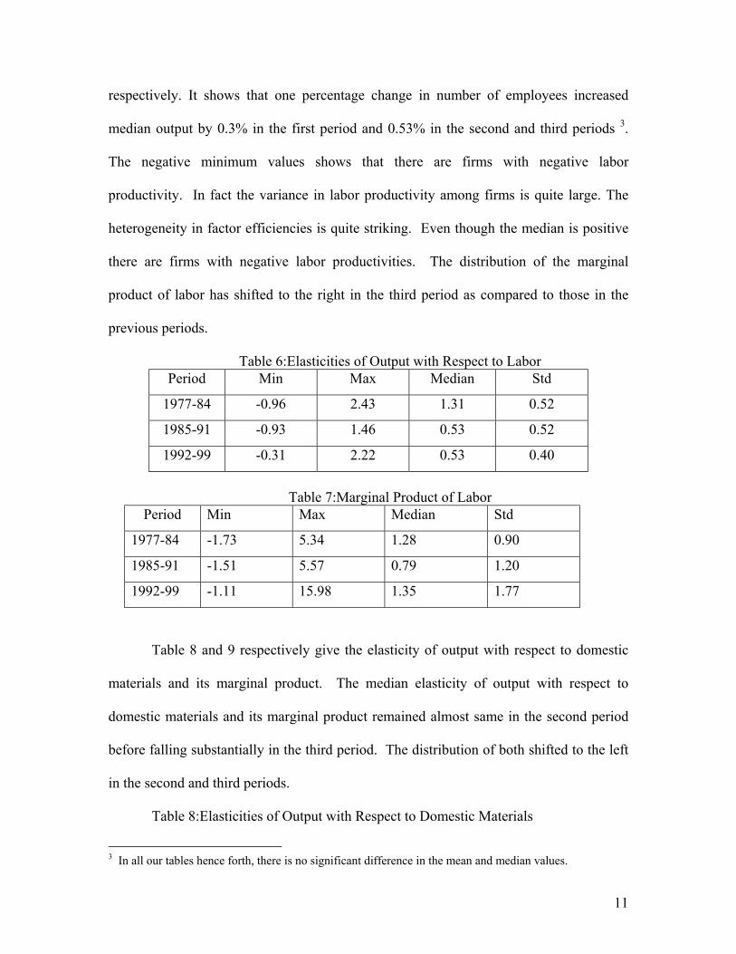
respectively. It shows that one percentage change in number of employees increased

median output by 0.3% in the first period and 0.53% in the second and third periods 3.

The negative minimum values shows that there are firms with negative labor

productivity. In fact the variance in labor productivity among firms is quite large. The

heterogeneity in factor efficiencies is quite striking. Even though the median is positive

there are firms with negative labor productivities. The distribution of the marginal

product of labor has shifted to the right in the third period as compared to those in the

previous periods.

Table 6:Elasticities of Output with Respect to Labor Period Min Max Median Std

1977-84 -0.96 2.43 1.31 0.52

1985-91 -0.93 1.46 0.53 0.52

1992-99 -0.31 2.22 0.53 0.40

Table 7:Marginal Product of Labor

Period Min Max Median Std

1977-84 -1.73 5.34 1.28 0.90

1985-91 -1.51 5.57 0.79 1.20

1992-99 -1.11 15.98 1.35 1.77

Table 8 and 9 respectively give the elasticity of output with respect to domestic

materials and its marginal product. The median elasticity of output with respect to

domestic materials and its marginal product remained almost same in the second period

before falling substantially in the third period. The distribution of both shifted to the left

in the second and third periods.

Table 8:Elasticities of Output with Respect to Domestic Materials

3 In all our tables hence forth, there is no significant difference in the mean and median values.

11

Period Min Max Median Std

1977-84 -0.49 1.61 0.37 0.39

1985-91 -0.83 1.48 0.38 0.41

1992-99 -0.89 1.06 0.06 0.35

Table 9:Marginal Product of Domestic Materials Period Min Max Median Std

1977-84 -2.04 4.57 0.80 0.81

1985-91 -19.20 3.34 0.78 1.83

1992-99 -39.16 2.11 0.13 3.00

Elasticity of output with respect to imported materials is shown in Table 10, is

found to be negative in the first and last periods while it is positive for the second period.

Surprisingly, the distribution has shifted substantially to the left in the last period. The

situation is different when we consider the distribution of marginal product of imported

material. The median value is the lowest in the third period but the distribution of

productivity in the third period has shifted substantially to the right as compared to the

second period but left as compared to the first period.

Table 10: Elasticities of Output with Respect to Imported Materials Period Min Max Median Std

1977-84 -0.43 0.54 -0.06 0.14

1985-91 -0.38 0.49 0.12 0.16

1992-99 -0.66 0.07 -0.23 0.15

Table 11:Marginal Product of Imported Materials Period Min Max Median Std

1977-84 -111.07 61.19 -0.54 11.82

12

1985-91 -366.75 4.43 0.91 35.07

1992-99 -156.16 21.26 -2.93 17.20

Elasticities of output with respect to capital are given in Table 12. It is negative

for the first period and positive and increasing for the second and third periods. Its

distribution has also been shifting to the right with the degree of liberalization. In Table

13 we see that marginal product of capital was extremely low when the economy was

closed. Even though the median value does not show substantial change, the distribution

of marginal product has significantly moved to the right.

Table 12: Elasticities of Output with Respect to Capital Period Min Max Median Std

1977-84 -0.53 0.54 -0.07 0.24

1985-91 -0.28 0.86 0.18 0.23

1992-99 -0.19 1.12 0.59 0.25

Table 13:Marginal Product of Capital Period Min Max Median Std

1977-84 -393.28 0.03 -0.01 28.59

1985-91 -0.15 0.52 0.01 0.07

1992-99 -0.01 2.29 0.02 0.31

Productivity growth rates:

Productivity of a firm at any point in time is given by exp(εit). It is computed by

replacing εit by the residual of the ith firm in year t. Tables 14 to 16 give productivity

growth rates of auto components industry for the three periods. Annual and period

averages of productivity growth rates for the industry are calculated as simple averages

13

and output share weighted growth rates of each of the firm’s in the sample. In the last

row of the table the period averages are given.

Table 14 gives the average productivity growth rates for the industry for the first

period. The simple averages of firm growth rates for the period show that productivity

increased by 3.2% during the first period while the weighted average productivity growth

rates show 2.61% for the same period. It implies that smaller firms experienced higher

growth rates than bigger firms in the auto components industry during 1977-84.

Table 14: Average Productivity Growth Rates in the Auto Components Industry During 1977-84. Year Simple

averages Weighted averages

1977-78 0.0312 0.0017

1978-79 0.0103 0.0084

1979-80 -0.0187 0.2005

1980-81 0.1235 0.0053

1981-82 0.0620 0.0115

1982-83 -0.0104 0.0294

1983-84 0.0234 -0.0738

1977-84 0.0316 0.0261

Table 15 gives the average productivity growth rates for the industry for the

second period. The simple average growth rates for the period show that productivity fell

on average by 0.01% while the weighted average productivity growth rates decreased by

4.34% in the second period. Again for smaller the firms productivity is lesser than that of

the bigger firms.

Table 15: Average Productivity Growth Rates in the Auto Components Industry During 1985-91.

14

Year Simple averages

Weighted averages

1985-86 -0.1152 -0.23

1986-87 -0.0007 -0.1457

1987-88 0.0834 0.3862

1988-89 0.0142 -0.0687

1989-90 0.0149 -0.1499

1990-91 -0.0310 -0.0525

1985-91 -0.0001 -0.0434

Productivity growth rates for the post 1991 period are shown in Table 16.

Contrary to the first two periods bigger firms performed better than the smaller firms in

terms of productivity growth rates. The simple average growth rates for the period are

1.09 % while the weighted average productivity growth rates are 4.25 %.

Table 16: Average Productivity Growth Rates in the Auto Components Industry During 1992-99. Year Simple

averages Weighted averages

1992-93 -0.0009 0.0656

1993-94 0.0212 -0.0475

1994-95 0.0288 0.1390

1995-96 0.0041 0.1274

1996-97 -0.0433 -0.0372

19997-98 0.0402 0.3130

1998-99 0.0262 -0.2629

1992-99 0.0109 0.0425

15

Productivity growth rates are found to be important contributors of output in the

first and third periods. In the second period it was not significant. This finding is in line

with the findings of previous studies 4.

5. Concluding Remarks

This paper attempts to learn about technological changes in the auto-components

industry when it moved from a restrictive policy regime to a less restrictive one in 1984

and finally to liberalized one in 1991. With regard to the factor efficiencies we find that

the middle period was more-or-less an adjustment period. Capital is the only factor for

which we find a monotonic relationship of its productivity with the degree of openness.

In all the periods we find that the productivities of all factors is very variable and firms

with negative factor productivities are not rare! This is perhaps a result of the fact that

losing concerns can not easily shutdown.

With regard to (neutral) productivity (TFP) changes we find that the closed

regime of the first period favored the smaller firms more whereas the most open regime

of the third period favors the bigger firms more leading to a higher growth in productivity

for the industry as a whole.

Currently we are trying to extend this study in two ways. One is to link it

to productivity movements in the auto industry. The other is to explicitly bring in the

role of imported capital.

4 Srivastava (1996) found that for the transport equipment and parts industry experienced productivity growth of –0.005 % for the period 1985-89. For the period between the years 1981 and 1984 he calculated this industry’s productivity growth as –0.010 %. In another relevant study by Krishna and Mitra (1998) productivity growth in the transport equipment industry is calculated as –0.000 % for the period between the years 1986 and 1993. Ahluwalia (1991) found 6.6% growth in productivity for the intermediate goods sector. Though panel data was used in this study the panel nature of the data was not modelled.

16

Data Appendix

The data used for the study are the firm-level panel data obtained from the

Reserve Bank of India for the period 1976-77 to 1989-99 inclusive. Company Finances

Department of Reserve Bank of India compiles these from the annual accounts of the

firms in the sector. From this data we have obtained the required variables as follows.

Output is defined as net sales adjusted for changes in inventories. Real output is

constructed by deflating output by the wholesale prices of main product of the firm.

Number of employees is taken as the labor variable. Amount spent on wages and salaries

is given in the data. We have collected per capita average wage of the public sector

employees and used it to divide wages and salaries figures to obtain number of

employees.

Regarding the domestic material input, domestic materials consumed are deflated

by wholesale price index of basic metals, alloys and metal products. Imported materials

variable is obtained by deflating the nominal expenditure on imported materials by unit

value index of imports of manufactures of metals.

Our data distinguishes between buildings and plant and machinery that together

account for about 95% of total gross capital stock. All calculations of the capital stock are

done separately for buildings and Plant and machinery. Real capital is obtained by

deflating gross capital stocks of buildings by wholesale price index of non metallic

mineral products and gross stocks of plant and machinery by wholesale price index of

heavy machinery. To calculate net stocks of capital, depreciation is calculated basing on

the straight-line depreciation method. For this purpose we considered the life span of

17

plant and machinery as 20 years and buildings as 50 years as suggested by Central

Statistical Organization (1989).

All the deflators used are constructed on 1981-82 base. We have collected all the price

indices from the Office of the Economic Adviser, Government of India, and Reserve

Bank of India Currency and Finance Report.

18

References: Ahluwalia, I.J., (1991) Productivity and Growth in Indian Manufacturing, Oxford University Press, Delhi. Arellano, M., and Bond, S., (1991) Some Tests of Specification for Panel Data: Monte Carlo Evidence and an Application to Employment Equations, Review of Economic Studies, 58, 277-297. Bardhan, P., and Lewis, S., (1970) Models of Growth with Imported Inputs, Economica, 371-385. Central Statistical Organization, Government of India, (1989) National Accounts Statistics: Sources and Methods, Department of Statistics, Ministry of Planning, New Delhi. Haddad M. (1991) How Trade Liberalization Effected Productivity in Morocco, World PRE working paper no. 1096. Harrison, A., (1994) Productivity, Imperfect Competition and Trade Reform: Theory and Evidence, Journal of International Economics, 36, 53-73. Jenkins Rhys (1995) Does Trade Liberalization led to Productivity Increases? A Case Study of Bolivian Manufacturing, Journal of International Development, 7, 577-597. Krishna, P., and Mitra, D., (1998) Trade Liberalization, Market Discipline and Productivity Growth: New Evidence from India, Journal of Development Economics, 56,447-462. Levinsohn, J., (1993) Testing the Imports-as-Market-Discipline Hypiothesis. Journal of International Economics 35, 1-22. Levinsohn, J., and Petrin, A., (1999) When Industries Become More Productive, Do Firms?: Investigating Productivity Dynamics, NBER Working Paper No.6893. Mulaga G. and Weiss J. (1996) Trade Reform and Manufacturing Performance in Malawi 1970-91, World Development, 24, 1267-1278. Mundlak, Y., (1996) Production Function Estimation: Reviving the Primal, Econometrica, 64 (2). Nishimizu M. and Robinson S. (1984) Trade Policies and Productivity Change in Semi-Industrializing Countries, Journal of Development Economics 16, 177-206. Office of Economic Adviser, Ministry of Industry, Index Numbers of Wholesale Prices in India, Various issues, Government of India, New Delhi. Olley, G.S., and Pakes, A.,( 1996) The Dynamics of Productivity in the Telecommunications Equipment Industry, Econometrica, 64(6), 1263-1297. Reserve Bank of India, Currency and Finance Report, Vol-2, Various issues, Mumbai.

19

Roberts, M.J., and Tybout, J.R., (1996) Industrial Evolution in Developing Countries, Oxford University Press. Tybout, J., (2000) Manufacturing Firms in Developing Countries: How Well They Do, and Why? Journal of Economic Literature, 38, 11-44. Srivastava, V., (1996) Liberalization, Productivity and Competition: A panel study of Indian Manufacturing, Oxford University Press, Delhi. Tybout, J.R., and Westbrook M.D., (1995) Trade Liberalisation and the Dimensions of Efficiency Change in Mexican Manufacturing Industries, Journal of International Economics, 39, 53-78. Weiss J. and Jayanthakumaran K. (1995) Trade Reforms and Manufacturing Performance: Evidence from Sri Lanka 1978-89, Development Policy Review, 13, 65-83.

20