discussion paper series product diversification and export

1

Discussion Paper Series

Product Diversification and Export Performance:

A Comparative Study of Developing Asian Countries

Alongkorn Tanasritunyakul

Discussion Paper No.64

November 18, 2021

International Competitiveness Research Center (ICRC) Faculty of Economics, Thammasat University

2

Product Diversification and Export Performance: A Comparative Study of Developing Asian Countries*

Alongkorn Tanasritunyakul

International Competitiveness Research Center (ICRC) Faculty of Economics, Thammasat University

[email protected] Abstract: There has been renewed emphasis in the recent trade policy debate on the

potential positive impact of diversification of the product composition on export expansion.

However, the standard trade theory predicts that export success depends on pursuing

comparative advantages rather than policy-induced export diversification. This paper

studies the relationship between product diversification and export performance of

developing Asian economies using panel data from 1976 to 2017. The methodology

involves estimating export equations for total non-oil exports and product subcategories.

Commodity diversification is alternatively measured using the Herfindahl-Hirschman and

Theil indices. The autoregressive distributed lag (ARDL) technique is used to delineate

short-run and long-run effects. The results suggest that export diversification has a negative

and statistically significant impact on export performance. This relationship holds for total

non-oil exports and the major exports subcategories. The magnitude of the impact varies for

product categories, casting doubt on the results of previous studies that focused on

aggregate exports. Supply-side factors appear to be more important than external demand in

explaining inter-country differences in export performance.

Keywords: Export diversification, International trade, Export performance

* This discussion paper is forthcoming in Thailand and The World Economy (TWE).

3

1. Introduction

The World economic slump and export contraction in the aftermath of the global

economic crisis of 2008 - 2009 has led to a renewed policy concern calling for export

diversification. It is widely believed that dependence on too few products can adversely

affect export growth. This concern is prominent in policy circles for both developed and

developing countries (Newfarmer, Shaw, & Walkenhorst, 2009; López-Cálix,

Walkenhorst, & Diop, 2010; Vos & Koparanova, 2011).

The case for the diversification of the product mix of exports of developing

countries is not new to the trade and development policy debate (Maizels, 2003). The

related literature dates back to the early 1950s when economic development in

developing countries emerged as a key theme in the economic profession (Prebisch,

1950; Singer, 1959). These studies were concerned with the decline in the term of trade

of developing countries resulting from the heavy concentration of exports in primary

products.

Some later studies came up with the idea of ‘Dutch disease’, alternatively called

the natural resource curse, which postulated the negative impact of natural resource

export on economic growth and non-natural resource exports (Corden, 1984; Gelb, 1988;

Sachs & Warner, 1999). The Dutch disease mechanism is that when there is a boom in

natural resource exports, this situation can raise wage levels and result in currency

appreciation. The latter effects deteriorate the price competition in non-natural resource

sectors such as manufacturing products. Thus, high dependence on natural resource

export is postulated to be potentially harmful to export performance.

In the context of renewed policy emphasis on export diversification, some

economists have recently argued that countries should be able to diversify exports

through industrial policy, that is, government policy targeted explicitly at industries, or

even individual firms, with export potential, to overcome the barriers to entry into export

markets (Hausmann & Rodrik, 2005; Rodrik, 2007). This literature based on the

perceived risk faced by ‘pioneer firms’ firms in “discovery of exports” and make a strong

case of the government engage in targeted industrial policy to eliminate barriers to entry.

When the pioneer firm succeeds in discovering a new export product, other firms can

obtain information from the pioneer firm and enter export markets.

4

The case for export diversification policy, however, is not consistent with the

standard trade theory: the Ricardian and the Heckscher-Ohlin models. These standard

trade theories postulate that export patterns should evolve naturally on specialization

based on countries’ comparative advantage. The international market is highly

competitive. Hence, specialization in a few products based on comparative advantage

would be more important for export success than diversification into many products

through direct policy intervention because specialization would help reap gains from

economies of scale and competitiveness in world markets.

There are, indeed, some vivid examples that export diversification may not

always guarantee faster export growth. For instance, India had a highly diversified export

basket that evolved through a protectionist trade regime during the first four decades of

the post-independent period. However, its share in world trade declined throughout this

period (Krueger, 2010). In contrast, some countries with less export diversification can

maintain considerable export growth. Hong Kong is such a particular case. Hong Kong

experienced rapid export growth with high commodity concentrations in textiles,

clothing, and footwear in the 1970s to the 1990s. The share of textiles, clothing, and

footwear exports accounted for over 60% of the total exports of Hong Kong during this

period (Weiss, 2005). Recent in-depth studies of emerging exports patterns in developing

countries have demonstrated that product-specific factors matter in export success over

and above policy-induced changes in the commodity mix (Hausmann & Rodrik, 2005;

Daruich, Easterly, & Reshef, 2019).

Besides, the rise in global production networks cast doubt on the validity of the

proposition that export diversification contributes to export expansion. This is because the

lead firms operating within global production networks set up production bases in

individual countries based on their relative cost advantage for specialization-specific

segments/tasks in the value chain. A given developing country is, therefore, not able to

determine its pattern of specialization within global production networks. It can only

create an enabling business environment to facilitate the process of specialization within

global production networks (Jones & Kierzkowski, 2001; Athukorala, 2014).

The advocacy of export diversification as a means of export expansion based on

the prior view that export diversification invariably promotes export growth. Only a few

studies have systematically tested this hypothesized relationship (Ali, Alwang, & Siegel,

1991; Roy, 1991; Piñeres & Ferrantino, 1997; Funke & Ruhwedel, 2001; Kandogan,

5

2006; Rosal, 2019). There are mixed results in the impact of export diversification on

export performance for developed and developing economies.

Therefore, the purpose of this paper is to examine the impact of export

diversification on export growth, drawing on the experiences of export performance

record in developing Asian countries over the period 1976-2017. These countries provide

an ideal laboratory for examining this issue because they have significant policy shifts

and structural changes in export patterns during this period.

This paper has some methodological improvements compared to the previous

studies. First, we cover a more prolonged period that can capture significant policy shifts

and structural changes in export patterns of the countries covered. The previous studies

covered much shorter periods (10 to 15 years), which is insufficient to capture the

dynamic of export diversification and its impact on export growth. Second, our empirical

analysis is undertaken for total non-oil exports and decomposing total non-oil exports into

commodity groups (primary products and manufactured products and major

subcategories within the latter). This disaggregation is needed because diversification

within different product groups can result in other impacts on export performance. Third,

we examine the implications of countries’ engagement in global production networks for

the relationship between commodity diversification and export growth. Finally, we

employ an econometric methodology that distinguishes between the short-run and long-

run (steady-state) relationships between export diversification and export growth.

The main finding of the paper is that product diversification is negatively

associated with export growth. This result holds for total non-oil merchandise exports,

primary exports, and manufactured exports. Thus, the findings are consistent with the

postulate of the standard trade theory that export success depends on specialization based

on comparative advantage in world trade rather than on product diversification achieved

through direct policy intervention.

The rest of the paper is structured as follows. Section 2 examines the trends and

patterns of commodity diversification and export performance. Section 3 describes the

estimation method and variables. Section 4 undertakes an econometric analysis of the

impact of commodity diversification on export performance. The final section

summarises the findings and makes policy inferences.

6

2. Trends and patterns of export diversification

2.1 Measurement of export diversification

There are two standard measures of export diversification: the Herfindahl-

Hirschman index (HHI) (Hirschman, 1964), and the Theil index (THI) (Theil, 1972).

The Herfindahl-Hirschman index (HHI) is

𝐻𝐻𝐻𝐻𝐻𝐻 =�∑ (𝑆𝑆𝑖𝑖)2𝑁𝑁

𝑖𝑖=1 −�1/𝑁𝑁

1−�1/𝑁𝑁 (1)

where si is the share of export in each product i and N is total product lines1. An

increase in the HHI represents concentration, while a decrease in the HHI indicates

diversification. In the extreme case, each product has the same export share; then, the

HHI is zero. By contrast, a country exports only one product; then the HHI is one.

The Theil index (THI) is defined as

𝑇𝑇𝐻𝐻𝐻𝐻 = 1𝑁𝑁∑ 𝑥𝑥𝑖𝑖

𝜇𝜇𝑁𝑁𝑖𝑖=1 𝑙𝑙𝑙𝑙 �𝑥𝑥𝑖𝑖

𝜇𝜇� and 𝜇𝜇 = 1

𝑁𝑁∑ 𝑥𝑥𝑖𝑖𝑛𝑛𝑖𝑖=1 (2)

where xi is the export value of product i and an N is the number of product lines.

A higher value of the THI indicates higher export concentration, while a lower value

reflects higher export diversification. The index ranges between 0 (extreme export

diversification) and the natural logarithm of N (extreme export concentration). Thus, the

Theil index can be normalized between 0 and 1 by dividing the natural logarithm of N.

The HHI is more sensitive to large export shares changes, which can result from

an economic crisis and demand and supply shocks because it is the sum of squared

export shares. By contrast, the THI is less susceptible to such extreme changes since it

measures each export's share relative to the average exports. The HHI is generally more

volatile than the THI. In the case of negatively skewed export data series, the numerical

value of the THI tends to be higher than that of the HHI (Cowell, 2000). Given these

differences, both indices are used in this paper for a robustness check.

1 Number of product lines refers to active exported products (excluding zero-valued exports) in

each country at each year because the prevalence of many zero-valued exports at the SITC 5-digit level are found in the case developing countries. So, this paper does not count zero-valued exports as number of product lines to avoid any bias in measuring the level of export diversification, especially developing countries with different stages of economic development.

7

Both indices are ‘indirect’ measures of diversification (‘direct’ measures of

concentration). Decreases in both indices (reflecting export diversification) can result

from two factors: an increase in numbers of new product lines and/or reduction of

export shares of existing products without new product lines.

2.2 Data compilation

The pattern of export diversification in developing Asian countries is examined

over the period 1976-2017. Data are compiled from the United Nation (UN) Comrade

database. Data based on the Revision 3 of Standard International Trade Classification

(SITC Rev. 3) is available for 1986 - 2018. Data are backdated to 1976 by linking data

based on the SITC Rev 2 for 1976-1985 to data based on SITC Rev. 3 using the SITC

Rev 3 – Rev 2 concordance available from the United Nation Statistical Office’s

website. Data for non-oil exports (Total exports – products belonging to SITC Section

3) are disaggregated into four subcategories (Table 1). Data on oil and gas products

(SITC 3) are excluded from this analysis's commodity coverage because exports of

these products depend on a country’s specific resource endowment. Not all countries

are thus able to diversify their export in oil and gas products. Also, price and volume

fluctuations of oil and gas products are significantly determined by non-market factors.2

2.3 Trends and patterns

The export structures of developing Asian countries have changed significantly

over the past five decades (Table 2). The shares of primary products in total exports

have declined, while manufactured goods account for an increasing share of export

composition. In the early 1980s, manufactured goods accounted for 46.8% of total

exports from developing Asian countries. This share had increased to 74.3% by

2016/17.

At the individual country level, this pattern is more prominent in East Asia and

Southeast Asia and South Asia, where, on average, manufactured goods account for 2 We perform the robustness check by estimating total merchandise exports including oil and gas products. According to the estimation results, the coefficient of diversification indices between total merchandise exports and total non-oil merchandise exports are not significantly different sign. However, the size of coefficient in the case of total merchandise export is greater than the coefficient of total non-oil merchandise.

8

over two-thirds of the total exports. In Southeast Asia, the only exception to this overall

pattern is Indonesia, where primary products still account for over 40% of total exports.

Interestingly, some developing countries with low per capita income have very high

export shares in manufactured products. For example, Bangladesh’s manufactured

products accounted for around 80% of total exports in 1990/91 and increased to about

96% of total exports in 2016/17. In Cambodia, the manufacturing share has remained

around 90% over the past two decades.

In Central and West Asia, primary products still account for the bulk of total

exports. Armenia has the highest primary export share in developing Asian countries,

with these products accounting for around 70% of total exports in 2016/17. In this

subregion, only two transition countries (Kazakhstan and Kyrgyzstan) have an upward

trend in their manufactured export shares in total exports (Table 2).

Data compiled to discuss the role of global production sharing exports within

global production networks (GPNs) in the export composition are summarized in Table

3. A comparison of data in Table 2 and 3 clearly shows that GPN exports are the key

factor in the upward trend of manufactured export shares. In the region as a whole, the

percentage of GPNs products in total manufacturing exports increased from 46.7% in

1980/81 to 65.0% in 2016/17. This evidence can be seen for all countries except India,

Pakistan, and Kazakhstan. The shares of GPN exports in total manufactured exports, on

average, in North Asia, Southeast Asia and South Asia were more than 60%, while the

shares of GPN exports in Central and West Asia was only 34.3% in 2016/17 (Table 3).

As some countries in South Asia, and Central and West Asia involving slightly

in global production networks, their GPN export shares account for less than 40% of

total manufactured exports. India is one example that is not able to engage in global

production networks. Compared with Bangladesh and Sri Lanka, India’s share of GPN

exports in total manufactured exports was very low, around 35% in 2016/17. On the

other hand, the shares of GPN exports in Bangladesh and Sri Lanka accounted for about

90% and 80% of total manufactured exports, respectively.

Data on export diversification patterns are summarized as measured by the

Herfindahl-Hirschman index (HHI), and the Theil index (THI) are plotted in Figure 1

and Figure 2, respectively. Table 4 reports only the Herfindahl-Hirschman index (HHI)

for each developing Asian country. To facilitate our analysis, both indices are reported

as percentages.

9

In general, both indices show the same export diversification pattern in total

exports, primary products, and the major export categories over the last three decades

(Figure 1 and Figure 2). The two indices are highly correlated3. However, there are two

vital differences between the HHI and the THI; the HHI is slightly more volatile than

the THI, and on average, the magnitude of the THI is relatively large than the HHI for

all commodity groups.

The export diversification levels in total non-oil exports and subcategories are

shown in Figure 1. In developing Asia, this region experienced a significant export

diversification in total non-oil exports. Its export diversification increased by

approximately 10% during the period 1980-2017. A comparison between primary

products and manufactured products shows that level of HHI in primary products, on

average, is higher (the degree of diversification is lower) than that of manufactured

products. This finding is consistent because the manufactured sector has more chances

of product diversification than primary products due to its higher range of product lines

and smaller resource constraints in domestic productions.

Patterns of export diversification reflect some responses to external shocks. For

example, after the Asian financial crisis of 1997-98, the degree of export diversification

dropped significantly; the HHI for total non-oil exports increased from 18.9% in 1997

to 23.1% in 1999 (Figure 1).

The data in Table 4 reveal the level of export diversification is different among

the four regions. On average, export diversification is highest in North Asia, followed

by Southeast Asia, South Asia, and Central and West Asia. Moreover, the enormous

changes in export diversification level for all four regions existed in 1980 to 2000. But

since 2000, export diversification has not been changing for all subregions. For

example, in total non-oil exports, the HHI’s South Asia was high at around 34.08% in

1980/81 and fell to 16.49% in 1995/96. However, after 2000, South Asia could not

substantially diversify its export basket.

GPN exports are generally more concentrated at the country level than non-GPN

exports for only the Asian countries with high engagement in global product sharing.

China is also such a case (Table 4 (e)). Compared with other commodity groups, export

diversification levels in China’s GPN products are low (the higher value in the HHI).

3 As the correlation calculation (not shown in this paper), we find that correlations between the HHI and the THI in each commodity group are around 0.90 - 0.97.

10

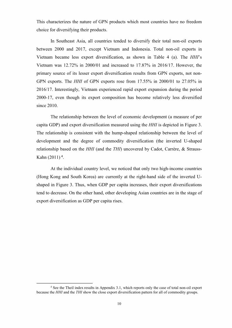
This characterizes the nature of GPN products which most countries have no freedom

choice for diversifying their products.

In Southeast Asia, all countries tended to diversify their total non-oil exports

between 2000 and 2017, except Vietnam and Indonesia. Total non-oil exports in

Vietnam became less export diversification, as shown in Table 4 (a). The HHI’s

Vietnam was 12.72% in 2000/01 and increased to 17.87% in 2016/17. However, the

primary source of its lesser export diversification results from GPN exports, not non-

GPN exports. The HHI of GPN exports rose from 17.55% in 2000/01 to 27.05% in

2016/17. Interestingly, Vietnam experienced rapid export expansion during the period

2000-17, even though its export composition has become relatively less diversified

since 2010.

The relationship between the level of economic development (a measure of per

capita GDP) and export diversification measured using the HHI is depicted in Figure 3.

The relationship is consistent with the hump-shaped relationship between the level of

development and the degree of commodity diversification (the inverted U-shaped

relationship based on the HHI (and the THI) uncovered by Cadot, Carrère, & Strauss-

Kahn (2011) 4.

At the individual country level, we noticed that only two high-income countries

(Hong Kong and South Korea) are currently at the right-hand side of the inverted U-

shaped in Figure 3. Thus, when GDP per capita increases, their export diversifications

tend to decrease. On the other hand, other developing Asian countries are in the stage of

export diversification as GDP per capita rises.

4 See the Theil index results in Appendix 3.1, which reports only the case of total non-oil export

because the HHI and the THI show the close export diversification pattern for all of commodity groups.

11

3. Econometric analysis

3.1 Model specification

This section aims to estimate a ‘reduced form’ export equation with export

diversification as an explanatory variable. The control variables are guided by previous

studies on export performances determinants (Goldstein & Khan, 1985; Bayar, 2018).

The export equation is specified as follow,

𝐸𝐸𝐸𝐸𝐸𝐸𝑖𝑖𝑖𝑖 = 𝛽𝛽0 + 𝛽𝛽1𝐷𝐷𝐻𝐻𝐷𝐷𝐸𝐸𝐷𝐷𝑖𝑖𝑖𝑖 + 𝛽𝛽2𝑊𝑊𝐷𝐷𝑖𝑖𝑖𝑖 + 𝛽𝛽3𝐺𝐺𝐷𝐷𝐸𝐸𝐺𝐺𝑖𝑖𝑖𝑖+𝛽𝛽4𝐷𝐷𝐸𝐸𝐸𝐸𝐷𝐷𝑖𝑖𝑖𝑖 + 𝛽𝛽5𝐹𝐹𝐷𝐷𝐻𝐻𝑖𝑖𝑖𝑖

+𝛽𝛽6𝑇𝑇𝐷𝐷𝑇𝑇𝐷𝐷𝐸𝐸𝑖𝑖𝑖𝑖+𝛽𝛽7𝐺𝐺𝐷𝐷𝐻𝐻𝐶𝐶𝐻𝐻𝐶𝐶𝑖𝑖𝑖𝑖 + 𝜀𝜀𝑖𝑖𝑖𝑖 (3)

where EXP is real exports (total non-oil exports and product subcategories), i =1,2,…,N

is the developing Asian countries, t = 1,2,…,T is the time unit in years. 𝜀𝜀 is the error

term in the model. The explanatory variables are listed below with the expected sign of

the regression coefficient in brackets:

DIVER (- / +) Export diversification alternatively measured by the HHI and the THI indices

WD (+) Real world demand measured as export-weighted GDP of trading partner countries (US$)

GDPC (+) Real per capita income of exporting country (US$)

REER (-) Real effective exchange rate

FDI (+) Real foreign direct investment (US$)

TRADE (+) Trade policy regime alternatively measured by openness index and trade liberalization index

CRISIS (-) Dummy variable for the global financial crisis taking value of 1 if year 2018-2019

WD is the real weighted income of export-destination countries. GDPC is real

per capita income representing the economic development stage, with higher GDPC

indicating the higher advanced stage of economic development. REER captures the

combined price effect of relative prices and exchange rate (export competitiveness). An

increase in REER implies a real appreciation of the domestic currency, which causes

export more expensive in export markets. FDI is real foreign direct investment (net

inflow), which influences the improvement in export supply capacity.

Trade policy regime (TRADE) is used by two indices: OPEN and LIB. OPEN is

trade openness measured as percentage shares of foreign trade (exports + imports) in

GDP. LIB is a trade liberalization index constructed by Sachs and Warner (1995) and

updated by Wacziarg and Welch (2008) and Paudel (2014). LIB represents trade

openness in terms of policy liberalization. Sachs and Warner (1995) state that a country

12

is classified as having open trade policy if a country exhibits the following five

characteristics: none of the average tariff rates of 40% or more on imports of

intermediate and capital goods, none of the non-tariff barrier covering 40% or more of

imports of intermediate and capital goods, none of black-market exchange rate

premium of 20% or more, none of a socialist economic system, and none of a state

monopoly on major export. We estimate the export model by using both indices for a

robustness check. The last variable (CRISIS) represents the effect of the global

financial crisis on exports in developing countries.

In this paper, we estimate the export equation as shown in equation (3) for total

non-oil exports and product subcategories for capturing the impact of export

diversification on export performance among product subcategories because of two

reasons. First, the stylized facts in section 2 show that the pattern of export

diversification level is determined by mixed patterns of export diversification in product

subcategories for some developing countries. For example, a decrease in export

diversification for Vietnam’s manufactured exports from 2000 to 2017 was from less

export diversification in GPN exports and higher export diversification in non-GPN

exports. Thus, we should investigate the effect of export diversification on export

growth for product subcategories, not only total non-oil exports. Second, the estimated

export equations for product subcategories can directly compare the impact of export

diversification on export growth among product subcategories such as GPN exports and

non-GPN exports.

3.2 Data

The model is estimated for total non-oil exports and four subcategories (primary

products, manufactured products, GPN products and non-GPN products) using panel

data for 20 developing Asian countries with a population of more than one million and

covers the period from 1976 to 2017. The panel data are unbalanced because of

limitations on data availability. Roughly, the sample coverage can be separated into

three groups (Table 5). The first group (10 countries) covers the starting years in the

late 1970s. The second group (2 countries) and the third group (8 countries) have the

starting years in the 1980s and the 1990s, respectively. The sample covers countries at

different economic development stages and includes natural-resource rich countries

such as Indonesia, Vietnam, and Kazakhstan. This would give considerable variability,

13

both over time in a given country and across countries, for econometric analysis on

commodity diversification's impact on export growth.

As already discussed in Section 2, data series for the dependent variable (total

non-oil exports and product subcategories) and export diversification index (HHI and

THI) are computed using data from the UN Comtrade database at SITC five-digit level.

We use export price (unit value) indices from the UNCTAD database to construct real

export series. However, export price indices are available at the SITC 3-digit level.

Thus, real export series in this paper are deflated at SITC 3-digit level for all product

subcategories.

Real world demand (WD) is measured by the weighted average of the real GDP

of the 20 major export destination countries of each developing Asian country. WD

varies by each country’s export market structure. We compute WD by using real GDP

at constant prices 2010 US$ from the World Bank database. GDPC is real GDP per

capita at constant prices 2010 US$ extracting from the World Bank database. FDI is

from the UNTAD database and is deflated by using GDP deflator for each country.

REER and the openness index are from the French Research Center in International

Economics (CEPII) and the World Bank database, respectively. Finally, LIB (policy

liberalization index) is from Sachs and Warner (1995), Wacziarg and Welch (2008),

and then Paudel (2014).

3.3 Estimation method

The traditional panel data estimation is not suitable for this study because of the

long-time span (t) in the panel dataset (Baltagi, 2001). Specifically, it could encounter a

spurious regression problem if the data series are non-stationary. It also fails to capture

possible differences between the short-run and long-run export diversification impact

on export growth. To avoid the above problems, we use the Autoregressive Distributed

Lag (ARDL) estimator (Pesaran, 2015).

The ARDL estimator can be used for the data series which are either stationary

at the level I(0) or stationary at the first difference I(1). The study uses the Fisher

combination test of Im, Pesaran, and Shin (2003), which applies to an unbalanced panel

dataset. This test method is also superior because it allows a heterogeneous panel

dataset with serially uncorrelated errors, unlike the traditional stationarity test, which

14

assumes a homogeneous panel dataset with serially uncorrelated errors. The stationarity

test results suggest that all data series are non-stationary at the level, but their first

differences are stationary (see Appendix B).

The export equation can be specified in ARDL with one period lag as following form,

1 2 3 4 5 6 7

1 1 2 1 3 1 4 1 5 1 6 1

7 1 1

it it it it it it it it

it it it it it it

it i it i it

EXP DIVER WD GDPC REER FDI TRADE CRISISDIVER WD GDPC REER FDI TRADECRISIS EXP

α α α α α α αα α α α α αα γ δ ε

− − − − − −

− −

= + + + + + +′ ′ ′ ′ ′ ′+ + + + + +′+ + + + (4)

where iδ is country specific effects, and itε is the error term. Given that X denotes all

exogenous variables in the model, except EXP. The error-correction formulation of

equation (4) is as follows:

1 1 1( )it i it i it i it i itEXP EXP X Xµ β λ δ ε− − −′ ′∆ = − + ∆ + + (5)

where 1it it itEXP EXP EXP −∆ = − , (1 )i iµ γ= − − , and 1

i ii

i

α αβγ′+′ =

−.

In equation (5), the short-run and long-run coefficients are represented as iλ′ and

iβ ′ , respectively. The study transforms all data series into the natural logarithm form,

except only LIB and CRISIS because both variables are dummy variables. Thus, the

coefficients can be explained as elasticity term. Besides, µ is the parameter of

adjustment toward the long-run equilibrium. To ensure a long run co-integration

relationship among the variables, µ must be negative and statistically significant.

One concern relating to the model specification as equation (5) is the possible

endogeneity problem in export value between two periods. However, the “ARDL

models have the advantage that they are robust to integration and co-integration

properties of the regressors, and for sufficiently high lag-orders could be immune to the

endogeneity problem, at least as far as the long-run properties of the model are

concerned” (Pesaran, 2015: p.726). This paper uses the Akaike information criterion

(AIC) as the criteria for choosing sufficiently high lags-order for ARDL estimation.

Based on the AIC, the optimal lag-orders for the dependent variable (p) and

independent variables (q) are two lags and one lag, respectively, for all cases except

primary products and GPN products. The latter cases are preferred to the one lag in the

dependent variable and independent variables.

15

The estimation allows heterogeneous characteristics in the panel dataset. We

estimate the export equation using the three alternative ARDL estimations: the Pooled

Mean Group estimator (PMGE), the Mean Group estimator (MGE), and the Dynamic

Fixed Effects estimator (DFEE). These estimations have different assumptions on short-

term and long-term coefficients. The PMG allows the short-term coefficients to differ

across groups, but the long-term coefficients are identical. However, the MG allows

both the short-term and long-term coefficients to differ across groups. The DFEE

imposes the constraints of identical coefficients in the short-term and long-term

coefficients for across groups.

To choose the preferred estimation among three alternative estimations, we

conduct the Hausman test. Regarding the Hausman test results in Appendix B, the

dynamic fixed effect estimation (DFEE) is the most preferred estimator.

4. Results

The results based on the DFEE estimator with HHI as the measure of

commodity diversification are reported in Table 6. The parameter of adjustment toward

the long-run equilibrium µ is negative and statistically significant. Thus, there is a

long-run cointegration relationship between the variables. The result of the alternative

estimate of the model with the Theil index (THI) is used in place of HHI for

comparison (see Appendix C). Since the two diversification indices are highly

correlated, the estimations with both indices have similar sign coefficients for all

explanatory variables5.

In Table 6, the adjustment coefficients are statistically significant in all

equations with the expected negative sign. This indicates that the model can capture the

long-term effect of the explanatory variables on export growth. The adjustment

coefficient varies in the rage of -0.15 to -0.35, suggesting that the speed of adjustment

varies significantly among the product categories. For example, there are vast

differences in speed of adjustment towards equilibrium between primary products and

5 The coefficients of export diversification index are positive and statistically significant for all

models using the HHI and the THI, except only the GPN model using the THI. However, the coefficients of the HHI model are lower than that of the THI. Also, there is no highly volatile measurement in export diversification when we use the HHI. Thus, the HHI model has reliable estimations and can be used as a baseline index.

16

manufactured products. The adjustment coefficient of primary products (-0.31) is

around twice as much as the manufactured products' coefficient (-0.15). Primary

products have a much slower speed of adjustment towards the long-run equilibrium

compared to manufactured products. Within manufacturing, non-GPN products have a

higher adjustment coefficient than GPN products. This suggests that GPN products

would respond better to any economic shock rather than non-GPN products. In the

following discussion, we specifically focus on the long-run regression coefficients

based on the adjustment coefficients.

The coefficient of the HHI, the key variable of interest, is positive and

statistically significant at the 1% level or better in all equations for the long-term effect.

In contrast, the short-term coefficient of the HHI is not statistically different from zero

in all cases. As expected, the relationship between commodity diversification and

export performance is effectually a long-term phenomenon.

Therefore, after controlling other variables, more export diversification is

associated with negative export growth for only the long-term effect. This result may be

surprising for some international trade economists. However, the result is consistent

with the evidence of India. India experienced a big improvement in export diversification

from 1980 to 2000, however, its export share in world market was constant at 0.6% of

world exports for the two decades. Moreover, the coefficients of export diversification

are different among product subcategories. For example, GPN products have a higher

coefficient of the HHI compared to non-GPN products. In Table 6, the HHI coefficients

are 0.414 and 0.282 for GPN products (column 7) and non-GPN products (column 9),

respectively. Thus, a decrease in commodity diversification by 1% would increase

export growth by 0.414% for GPN products and 0.282% for non-GPN products.

To comment on the control variables' results, the dummy variable for the global

financial crisis (CRISIS) has a negative long-term effect on export growth as expected.

The trade openness coefficient measured by the trade to GDP ratio is statically

significant with the expected positive sign in all equations. However, the Sachs-Werner

index's coefficient, which is used as an alternative measure of trade openness, is not

statistically significant in all regressions even though it carries the positive sign as

expected. This is presumably because a binary variable does not have sufficient

variation over time.

17

The impact of world demand on export growth is positive for all product

subcategories except primary products. In other words, an increase in world demand

results in export growth in the long run. However, Table 6 shows that the coefficients of

world demand are distinct among product subcategories. Comparing GPN products and

non-GPN products, the coefficients of world demand are 0.520 (column 7) and 0.168

(column 9), respectively. As a result, GPN products would respond more to an increase

in world demand than non-GPN products. This result confirms the importance of GPN

products in export success in developing Asian countries.

The REER coefficient is negative and statistically significant in the long run for

total non-oil exports and all product subcategories. As expected, real exchange rate

appreciation leads to lower export performance. Interestingly, the degree of long-run

responsiveness of GPN products (-0.884) is much smaller compared to that of non-GPN

products (-1.198). This difference is consistent with the postulate that exports based on

global production sharing are relatively less responsive to relative price changes (as the

overall production structure is dispersed among many countries) compared to export

based on the traditional form of horizontal specialization (Athukorala & Khan, 2016).

On the supply side, GDP per capita is a vital factor determining export

performance in developing Asian countries. The coefficient of GDPC is significant at

the 1% level, and it is the largest coefficient compared to that of other explainable

variables. The long-term coefficients range between 0.7 and 1.7, while the short-term

coefficients range between 1.0 and 2.9. Notably, the coefficients of GDPC are

statistically significant for all cases. Thus, the stage of economic development is

essential for improving export performance.

Also, the FDI coefficient is positive and statistically significant at the 1% level

in the short-run and the long-run for only GPN products. Unsurprisingly, most FDI

inflow in Asia is relevant to global production sharing. An increase in FDI inflow is

associated with higher export growth for GPN products. Thus, FDI inflow is one

important channel to boost export performance for the short-run and the long-run.

Lastly, the results suggest that GDP per capita, which captures the country's

state of development, is much more important than world demand in explaining export

performance. This result is consistent with the standard small-country assumption

relating to export performance (Athukorala & Riedel, 1996). Thus, the role of supply

capability is vital for export expansion. Interestingly, alternative estimates suggest that

18

the results are remarkably resilient to the exclusion of the world demand variable from

the model (see Appendix C, Table C.2).

5. Conclusion This paper has examined the relationship between export product diversification

and export performance in developing Asian countries. The analysis covered total non-

oil exports distinguishing between primary products and manufactured products, with

the latter further disaggregated into exports within global production networks (GPN

products) and non-GPN products.

The key finding is that export diversification has a negative impact on export

performance for total exports and all product subcategories in developing Asian

countries. This result is consistent with some previous studies. For example, Piñeres

and Ferrantino (1997) provided evidence of a negative association between export

growth and export diversification in Chile. Also, export diversification in new products

did not contribute much to export growth in developing countries (Newfarmer et al.,

2009). Thus, the result in this paper supports the prediction of the standard trade theory,

which postulates that a country gains from international trade by specialization based

on its own comparative advantage.

This paper does not suggest that developing countries should not diversify their

exports. However, developing countries should realize that export diversification does

not guarantee higher export growth. One reason is that high export performance can

occur when a country can diversify its exports toward new potential products in the

world market. Second reason is that a country should diversify its exports based on its

comparative advantage in each stage of economic development.

In conclusion, our estimation results suggest that government should facilitate

and improve the attractiveness of foreign direct investment for improving export supply

capacity and promoting potential exported products with corresponding a country’s

comparative advantage. In particular, GPN products should be targeted for developing

countries because GPN exports can highly grow with world demand compared to other

product subcategories.

19

Table 1: Definition of commodity group

No. Commodity group SITC Codes 1 Total non-oil

Item 1 + 2 2 Primary products SITC section 0, 1, 2, 4 and 68 excluding oil and gas

3 Manufactured

SITC section 5, 6 (less SITC 68: nonferrous metals), 7,

4 GPN products See Athukorala (2019) 5 Non-GPN products Item 3 - 4 Note: 1 Manufactured products are comprised of GPN products and Non-GPN products. Source: Author’s compilation.

Table 2: Shares of manufactured products in total non-oil exports (%)1

1980/8

1990/9

1995/9

2000/0

2005/0

2010/1

2016/1 North Asia 91.8 89.6 92.3 94.4 95.6 94.5 94.8

China n.a. 80.7 87.6 91.5 94.3 94.7 94.9 Hong Kong 92.9 93.4 93.9 95.9 96.8 94.2 94.7 South Korea 90.7 94.7 95.3 95.9 95.8 94.6 94.7 Southeast Asia 32.0 72.3 82.2 86.2 84.3 79.6 82.4 Brunei n.a. 81.3 98.9 99.2 94.1 96.2 95.5 Cambodia n.a. n.a. n.a. 96.3 97.6 94.9 93.0 Indonesia 11.7 64.7 68.5 76.1 62.9 51.0 57.0 Malaysia 26.0 69.1 82.4 89.7 87.2 73.9 74.9 Philippines 27.7 64.4 77.1 92.4 90.1 80.0 86.2 Singapore 70.0 88.6 92.7 95.7 94.1 93.0 91.8 Thailand 24.4 65.8 73.8 79.4 81.0 76.0 79.0 Vietnam n.a. n.a. n.a. 60.6 67.6 71.4 82.0

South Asia 45.8 73.5 81.3 84.4 82.0 79.6 81.9 Bangladesh 68.1 80.0 87.2 91.9 91.9 93.6 96.4 India 45.2 74.0 75.0 81.5 78.7 78.6 81.2 Pakistan2 58.7 80.2 84.3 86.6 85.5 77.0 77.9 Sri Lanka 11.3 59.8 78.8 77.5 72.0 69.2 72.3

Central and West

n.a. n.a. 46.1 41.0 49.3 47.2 42.9 Armenia3 n.a. n.a. 56.4 62.6 68.4 33.6 29.4 Azerbaijan n.a. n.a. 58.4 44.7 42.3 44.1 32.7 Georgia n.a. n.a. 50.0 36.1 44.0 62.0 48.2 Kazakhstan n.a. n.a. 19.8 16.6 35.5 42.3 44.8 Kyrgyzstan n.a. n.a. 46.1 45.1 56.5 54.0 59.6 Developing Asia 46.8 76.7 73.7 75.8 76.8 73.7 74.3 Note: 1. n.a. denotes non-available data. 2. Due to the lack of observation in 1980/81 for Pakistan, we use observation in 1982 instead of 1980/81. 3. Due to the lack of observation in 1995/96 for Armenia, we use observation in 1997 instead of 1995/96. Source: Author’s computation using the UN Comtrade database.

20

Table 3: Shares of GPN Products in total manufactured exports (%)1

1980/8

1990/9

1995/9

2000/0

2005/0

2010/1

2016/1 North Asia 65.8 67.3 65.0 70.3 73.6 68.7 67.0

China n.a. 63.0 61.4 68.1 70.2 65.9 62.0 Hong Kong 74.6 72.1 68.5 73.1 78.2 74.0 75.1 South Korea 57.0 66.9 65.1 69.6 72.3 66.3 64.0 Southeast Asia 59.7 67.6 67.5 77.1 72.6 63.0 66.1 Brunei n.a. n.a. 46.2 81.0 79.2 54.7 41.8 Cambodia n.a. n.a. n.a. 79.2 78.3 67.8 92.3 Indonesia 40.4 36.2 45.3 52.1 51.5 49.8 49.0 Malaysia 75.1 80.5 79.2 82.2 77.2 65.2 63.1 Philippines 55.7 73.6 83.0 93.3 91.4 82.3 86.2 Singapore 71.0 77.3 81.9 81.8 65.4 61.3 58.1 Thailand 56.1 70.6 69.4 69.9 66.8 57.8 60.9 Vietnam n.a. n.a. n.a. 77.1 71.2 64.8 77.3


Central and West

n.a. n.a. 25.6 33.9 31.0 32.5 34.3 Armenia3 n.a. n.a. 28.0 24.5 9.7 15.7 34.3 Azerbaijan n.a. n.a. 29.1 50.5 47.1 25.0 18.9 Georgia n.a. n.a. 15.9 37.8 41.7 44.6 37.3 Kazakhstan n.a. n.a. 25.0 10.1 15.1 7.0 11.9 Kyrgyzstan n.a. n.a. 30.0 46.5 41.5 70.1 69.0 Developing Asia 46.7 61.4 52.5 61.6 59.1 54.9 65.0 Note: 1. n.a. denotes non-available data. 2. Due to the lack of observation in 1980/81 for Pakistan, we use observation in 1982 instead of 1980/81. 3. Due to the lack of observation in 1995/96 for Armenia, we use observation in 1997 instead of 1995/96. Source: Author’s computation using the UN Comtrade database.

21

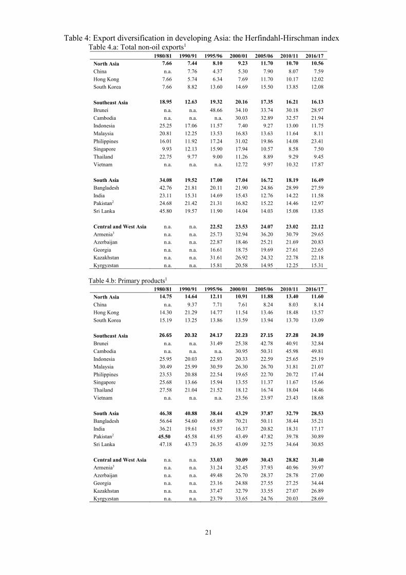
Table 4: Export diversification in developing Asia: the Herfindahl-Hirschman index Table 4.a: Total non-oil exports1

1980/81 1990/91 1995/96 2000/01 2005/06 2010/11 2016/17

North Asia 7.66 7.44 8.10 9.23 11.70 10.70 10.56 China n.a. 7.76 4.37 5.30 7.90 8.07 7.59 Hong Kong 7.66 5.74 6.34 7.69 11.70 10.17 12.02 South Korea 7.66 8.82 13.60 14.69 15.50 13.85 12.08 Southeast Asia 18.95 12.63 19.32 20.16 17.35 16.21 16.13 Brunei n.a. n.a. 48.66 34.10 33.74 30.18 28.97 Cambodia n.a. n.a. n.a. 30.03 32.89 32.57 21.94 Indonesia 25.25 17.06 11.57 7.40 9.27 13.00 11.75 Malaysia 20.81 12.25 13.53 16.83 13.63 11.64 8.11 Philippines 16.01 11.92 17.24 31.02 19.86 14.08 23.41 Singapore 9.93 12.13 15.90 17.94 10.57 8.58 7.50 Thailand 22.75 9.77 9.00 11.26 8.89 9.29 9.45 Vietnam n.a. n.a. n.a. 12.72 9.97 10.32 17.87


Central and West Asia n.a. n.a. 22.52 23.53 24.07 23.02 22.12 Armenia3 n.a. n.a. 25.73 32.94 36.20 30.79 29.65 Azerbaijan n.a. n.a. 22.87 18.46 25.21 21.69 20.83 Georgia n.a. n.a. 16.61 18.75 19.69 27.61 22.65 Kazakhstan n.a. n.a. 31.61 26.92 24.32 22.78 22.18 Kyrgyzstan n.a. n.a. 15.81 20.58 14.95 12.25 15.31

Table 4.b: Primary products1

1980/81 1990/91 1995/96 2000/01 2005/06 2010/11 2016/17




22

Table 4.c: Manufactured products1

1980/81 1990/91 1995/96 2000/01 2005/06 2010/11 2016/17

North Asia 8.04 8.12 8.48 9.54 12.04 11.14 10.98 China n.a. 9.45 4.80 5.64 8.22 8.35 7.83 Hong Kong 7.96 5.79 6.53 7.82 11.88 10.60 12.52 South Korea 8.11 9.13 14.10 15.15 16.01 14.48 12.59 Southeast Asia 17.07 15.02 20.70 21.41 17.92 16.37 17.24 Brunei n.a. n.a. 49.07 34.32 35.39 31.18 30.19 Cambodia n.a. n.a. n.a. 31.05 33.53 34.09 23.21 Indonesia 24.68 24.29 13.35 7.49

6.61 6.69 8.29

Malaysia 18.75 13.59 15.12 18.48 15.12 11.09 8.36 Philippines 10.07 13.53 19.98 33.47 21.85 16.85 27.06 Singapore 8.88 13.53 16.99 18.61 11.07 9.06 7.94 Thailand 22.95 10.18 9.66 13.45 10.30 10.82 11.39 Vietnam n.a. n.a. n.a. 14.42 9.51 11.14 21.49



Table 4.d: GPN products1

1980/81 1990/91 1995/96 2000/01 2005/06 2010/11 2016/17




23

Table 4.e: Non-GPN products1

1980/81 1990/91 1995/96 2000/01 2005/06 2010/11 2016/17




Note: 1 n.a. denotes non-available data. 2 Due to lack of observation in 1980/81 for Pakistan, we use observation in 1982 instead of 1980/81. 3 Due to lack of observation in 1995/96 for Armenia, we use observation in 1997 instead of 1995/96. Source: Author’s computation using the UN Comtrade database.

Table 5: List of developing Asian countries

Time range Number of countries List of country

The late 1970s - 2017 10 Bangladesh, Hong Kong, India, Indonesia, South Korea, Malaysia, Philippines, Sri Lanka, Singapore, Thailand

The 1980s - 2017 2 China, Pakistan The late 1990s - 2017 8 Armenia, Azerbaijan, Brunei, Cambodia, Georgia,

Kazakhstan, Kyrgyzstan, Vietnam Source: Author’s compilation from the list of developing countries based on the UN country classification.

24

Table 6: The estimation results based on the Herfindahl-Hirschman index (HHI) Dependent var. Total non-oil Primary Manufacture

GPN Non-GPN

(Real export) (1) (2) (3) (4) (5) (6) (7) (8) (9) (10)

Long-run Coefficients

HHI t-1 0.241*** 0.395*** 0.473*** 0.498*** 0.391*** 0.548*** 0.414* 0.494** 0.282*** 0.284***

(0.002) (0.000) (0.079) (0.084) (0.003) (0.058) (0.241) (0.244) (0.016) (0.025)

World demand t-1 0.009 0.059 -0.255*** -0.235*** 0.169* 0.199* 0.520*** 0.494*** 0.168*** 0.103

(0.086) (0.137) (0.017) (0.007) (0.099) (0.114) (0.027) (0.046) (0.038) (0.128)

GDPC t-1 1.245*** 1.306*** 1.280*** 1.261*** 1.125*** 1.208*** 0.900*** 0.994*** 1.632*** 1.763***

(0.137) (0.203) (0.203) (0.202) (0.125) (0.191) (0.158) (0.105) (0.199) (0.287)

FDI t-1 0.087* 0.107 0.078** 0.084*** 0.087* 0.134 0.207*** 0.255*** 0.027 0.037

(0.051) (0.095) (0.038) (0.031) (0.049) (0.092) (0.057) (0.020) (0.113) (0.121)

REERt-1 -0.481*** -0.864*** -0.417*** -0.564*** -0.360** -0.894*** -0.884*** -1.076*** -1.198*** -1.331***

(0.136) (0.192) (0.063) (0.064) (0.155) (0.065) (0.153) (0.093) (0.157) (0.026)

OPENNESS t-1 0.615*** 0.139*** 0.883*** 0.687*** 0.487**

(0.109) (0.042) (0.084) (0.117) (0.217)

LIBER 0.264 0.031* 0.236 0.063 0.209

(0.422) (0.017) (0.458) (0.161) (0.219)

CRISIS -0.337*** -0.532*** -0.139*** -0.253*** -0.315*** -0.550*** -0.515*** -0.484*** -0.191*** -0.166

(0.059) (0.197) (0.017) (0.004) (0.074) (0.096) (0.131) (0.036) (0.050) (0.110)

Adjustment coefficient -0.155*** -0.157*** -0.311*** -0.314*** -0.150*** -0.152*** -0.235*** -0.228*** -0.263*** -0.258***

(0.042) (0.026) (0.011) (0.010) (0.018) (0.006) (0.015) (0.018) (0.069) (0.065)

Short-run Coefficients

∆HHI 0.204 0.186 -0.084 -0.098 0.109 0.092 0.028 0.023 0.236 0.245

(0.246) (0.244) (0.059) (0.061) (0.174) (0.180) (0.173) (0.162) (0.265) (0.272)

∆World demand 0.033 0.006 0.091*** 0.083*** 0.040 0.008 0.089*** 0.082*** -0.070 -0.076

(0.101) (0.107) (0.026) (0.029) (0.119) (0.130) (0.001) (0.010) (0.045) (0.065)

∆GDPC 0.935*** 0.990*** 0.376*** 0.386*** 1.387*** 1.463*** 1.805*** 1.882*** 1.023*** 1.046***

(0.035) (0.011) (0.064) (0.037) (0.001) (0.022) (0.011) (0.001) (0.217) (0.227)

∆FDI -0.006 -0.000 0.011** 0.017*** -0.004 0.001 0.051*** 0.046*** 0.018*** 0.016

(0.009) (0.001) (0.005) (0.004) (0.013) (0.004) (0.017) (0.008) (0.006) (0.011)

∆REER -0.184 -0.292*** 0.007 -0.008 -0.250** -0.358*** -0.006 0.001 -0.198 -0.164**

(0.136) (0.057) (0.008) (0.009) (0.118) (0.017) (0.008) (0.002) (0.137) (0.069)

∆OPENNESS 0.400** 0.419*** 0.449* -0.178 -0.132

(0.176) (0.027) (0.233) (0.295) (0.228)

∆LIBER -0.024 -0.170*** -0.034 -0.047*** 0.095

(0.061) (0.009) (0.049) (0.018) (0.070)

∆CRISIS -0.037 -0.017 -0.030*** -0.010 -0.032 -0.008 0.034 0.036** -0.022 -0.019

(0.038) (0.040) (0.003) (0.006) (0.032) (0.037) (0.030) (0.015) (0.035) (0.046)

∆EXP at t-1 0.045 0.063 0.048*** 0.064*** 0.058 0.061

(0.063) (0.050) (0.012) (0.007) (0.083) (0.078)

Constant -0.156 0.342 0.925* 1.294*** -0.655*** 0.098*** -1.441*** -0.653*** -0.985*** -0.339**

(0.313) (0.217) (0.476) (0.377) (0.163) (0.015) (0.241) (0.231) (0.226) (0.152)

Observations 621 621 621 621 621 621 621 621 621 621 Note: ***, **, * respectively denotes 1%, 5%, and 10% level of significance. The standard errors are reported in parentheses. Source: Author’s estimation.

25

Figure 1: Export diversification in developing Asia: the Herfindahl-Hirschman index1

Figure 1 (a): Total exports, primary and manufactured products

Figure 1 (b): GPN and non-GPN products

Note: 1 The values are simple average of the Herfindahl-Hirschman index (HHI). Source: Author’s computation using the UN Comtrade database.

Figure 2: Export diversification in developing Asia: the Theil index1

Figure 2 (a): Total exports, primary and manufactured products

Figure 2 (b): GPN and non-GPN products

Note: 1 The values are simple average of the Theil index (THI). Source: Author’s computation using the UN Comtrade database.

10

20

30

40

1980 1985 1990 1995 2000 2005 2010 2015

total export primary products manufactured products

10

20

30

40

1980 1985 1990 1995 2000 2005 2010 2015

GPN Non-GPN

30

40

50

60

1980 1985 1990 1995 2000 2005 2010 2015

total export primary products manufactured products

30354045505560

1980 1985 1990 1995 2000 2005 2010 2015

GPN Non-GPN

26

Figure 3: Export diversification in total non-oil exports (measured by the HHI) and GDP per capita in developing Asian countries in the period 1976-2017

Source: The Herfindahl-Hirschman index (HHI) is estimated using data from the UN Comtrade database, and data on GDP per capita are from World Development Indicators, World Bank.

020

4060

HH

I (pe

rcen

t)0 10000 20000 30000 40000

GDP per capita (US$)

27

References

Ali, R., Alwang, J. R., & Siegel, P. B. (1991). Is export diversification the best way to achieve export growth and stability?: A look at three African countries, World Bank Policy Research Working Paper Series No. 729.

Athukorala, P. (2014). Global production sharing & trade patterns in East Asia. In I. Kaur, & N. Singh (Eds.), Oxford Handbook of Pacific Rim Economies (pp. 334-360). New York: Oxford University Press.

Athukorala, P., & Khan, F. (2016). Global production sharing and the measurement of price elasticity in international trade. Economics Letters, 139(C), 27-30.

Athukorala, P., & Riedel, J. (1996). Modelling NIE exports: Aggregation, quantitative restrictions and choice of econometric methodology. The Journal of Development Studies, 33(1), 81-98.

Baltagi, B. H. (2001). Econometric analysis of panel data (2nd ed.). New York: John Wiley & Sons.

Bayar, G. (2018). Estimating export equations: A survey of the literature. Empirical Economics, 54(2), 629-672.

Cadot, O., Carrère, C., & Strauss-Kahn, V. (2011). Export diversification: What's behind the hump?. Review of Economics and Statistics, 93(2), 590-605.

Corden, W. M. (1984). Booming sector and Dutch disease economics: Survey and consolidation. Oxford Economic Papers, 36(3), 359-380.

Cowell, F. A. (2000). Measurement of inequality. In A.B. Atkinson & F. Bourguignon, Handbook of Income Distribution, Volume 1 (pp. 87-166). Oxford, United Kingdom: Elsevier.

Daruich, D., Easterly, W., & Reshef, A. (2019). The surprising instability of export specializations. Journal of Development Economics, 137(1), 36-65.

Funke, M., & Ruhwedel, R. (2001). Export variety and export performance: Empirical evidence from East Asia. Journal of Asian Economics, 12(4), 493-505.

Gelb, A. H. (1988). Oil windfalls: Blessing or curse?. New York: Oxford University Press.

Goldstein, M., & Khan, M.S. (1985). Income and price effects in foreign trade. In R.W. Jones & P.B. Kenen (Eds.), Handbook of International Economics, Vol. II (pp. 1041-1105). New York: Elsevier Science Publications.

Hausmann, R., & Rodrik, D. (2005). Self-discovery in a development strategy for El Salvador. Economía, 6(1), 43-101.

Hirschman, A. O. (1964). The paternity of an index. The American Economic Review, 54(5), 761–762.

Im, K. S., Pesaran, M. H., & Shin, Y. (2003). Testing for unit roots in heterogeneous panels. Journal of econometrics, 115(1), 53-74.

Jones, R. W., & Kierzkowski, H. (2001). Globalization and the consequences of international fragmentation. In G. A. Calvo, R. Dornbusch & M. Obstfeld (Eds.), Money, capital mobility, and trade: Essays in honor of Robert A. Mundell (pp. 365-383). Massachusetts: The MIT Press.

Kandogan, Y. (2006). Does product differentiation explain the increase in exports of transition countries?. Eastern European Economics, 44(2), 6-22.

Krueger, A. O. (2010). India’s trade with the world: Retrospect and prospect. In S. Acharya, & R. Mohan (Eds.), India’s economy: Performances and challenges–Essays in honour of Montek Singh Ahluwalia (pp. 399-429). New Delhi, India: Oxford University Press.

28

López-Cálix, J. R., Walkenhorst, P., & Diop, N. (Eds.). (2010). Trade competitiveness of the Middle East and North Africa: Policies for export diversification. Washington DC: The World Bank.

Maizels, A. (2003). Economic dependence on commodities. In J. F. Toy (Ed), Trade and development: Directions for the 21st century (pp. 169-184). Cheltenham, United Kingdom: Edward Elgar.

Newfarmer, R., Shaw, W., & Walkenhorst, P. (Eds.). (2009). Breaking into new markets: Emerging lessons for export diversification?. Washington DC: The World Bank.

Paudel, R., (2014). Trade liberalization and economic growth in developing countries: Does stage of development matter?. Crawford School of Public Policy Working Paper. The Australian National University. Retrieved from https://papers.ssrn.com/sol3/papers.cfm?abstract_id=2545735

Pesaran, M. H. (2015). Time series and panel data econometrics. New York: Oxford University Press.

Piñeres, S. A. G., & Ferrantino, M. (1997). Export diversification and structural dynamics in the growth process: The case of Chile. Journal of Development Economics, 52(2), 375-391.

Prebisch, R. (1950). The economic development of Latin America and its principal problems, economic commission for Latin America. New York: United Nations.

Rodrik, D. (2007). One economics, many recipes: Globalization, institutions, and economic growth. Princeton, United Kingdom: Princeton University Press.

Rosal, D. I. (2019). Export diversification and export performance by destination country. Bulletin of Economic Research, 71(1), 58-74.

Roy, D. K. (1991). Determinants of export performance of Bangladesh. The Bangladesh Development Studies, 19(4), 27-48.

Sachs, J. D., & Warner, A. M. (1995). Economic reform and the process of global integration. Brookings Papers on Economic Activity, 1, 1-118.

Sachs, J. D., & Warner, A. M. (1999). The big push, natural resource booms and growth. Journal of Development Economics, 59(1), 43-76.

Singer, H. W. (1959). Stabilization and development of primary producing countries. Kyklos, 12(2), 271-283.

Theil, H. (1972). Statistical decomposition analysis with applications in the social and administrative sciences. Amsterdam, Netherlands: North Holland Publishing.

Vos, R., & Koparanova, M. (Eds.) (2011). Globalization and economic diversification: Policy challenges for economies in transition. London, United Kingdom: Bloomsbury Academic.

Wacziarg, R., & Welch, K. H. (2008). Trade liberalization and growth: New evidence. The World Bank Economic Review, 22(2), 187-231.

Weiss, J. (2005). Export growth and industrial policy: Lessons from the East Asian miracle experience. ADB Institute Discussion Papers No. 26.

29

Appendix A

Table A.1: Export diversification pattern by the Theil index1

Total non-oil export 1980/81 1990/91 1995/96 2000/01 2005/06 2010/11 2016/17

North Asia 29.15 26.97 26.34 28.30 32.11 30.48 29.96

China n.a. 26.48 20.43 21.85 24.97 23.65 22.67

Hong Kong 28.06 24.24 25.28 27.80 33.28 32.06 34.66

South Korea 30.23 30.19 33.32 35.25 38.08 35.73 32.54

Southeast Asia 46.98 35.78 42.22 44.88 42.19 40.14 38.69

Brunei n.a. n.a. 70.87 61.83 60.34 53.55 52.00

Cambodia n.a. n.a. n.a. 62.22 65.13 63.00 53.88

Indonesia 57.46 38.60 34.00 28.90 30.70 34.95 32.90

Malaysia 51.60 37.65 38.10 40.11 37.30 32.75 28.60

Philippines 44.36 37.65 42.51 53.97 48.75 43.14 45.84

Singapore 28.74 31.09 36.57 40.46 30.23 29.38 28.98

Thailand 52.72 33.93 31.24 31.53 30.18 30.28 29.69

Vietnam n.a. n.a. n.a. 40.03 34.86 34.06 37.61

South Asia 64.08 48.68 45.52 45.01 43.48 44.56 42.89

Bangladesh 75.90 58.24 55.16 55.87 55.91 58.62 58.06

India 53.82 36.36 34.14 32.38 30.23 32.10 28.97

Pakistan2 51.32 51.64 51.03 47.85 44.11 42.18 41.52

Sri Lanka 75.30 48.48 41.75 43.94 43.67 45.35 43.02

Central and West Asia n.a. n.a. 50.77 51.96 53.69 53.50 51.22

Armenia3 n.a. n.a. 52.05 57.58 64.08 61.45 57.84

Azerbaijan n.a. n.a. 48.36 49.02 55.00 53.93 52.65

Georgia n.a. n.a. 47.18 50.28 52.10 57.14 52.15

Kazakhstan n.a. n.a. 60.06 55.84 53.82 54.30 50.46

Kyrgyzstan n.a. n.a. 46.20 47.06 43.44 40.69 43.01 Note: 1 n.a. denotes non-available data. 2 Due to lack of observation in 1980/81 for Pakistan, we use observation in 1982 instead of 1980/81. 3 Due to lack of observation in 1995/96 for Armenia, we use observation in 1997 instead of 1995/96. Source: Author’s computation using the UN Comtrade database.

30

Appendix B Table B.1: Results of the unit root test

Variable Level I(0) First Difference I(1) W-t-bar p-value W-t-bar p-value Real Export Total non-oil merchandise 3.2043 0.9993 -7.0074 0.0000 Total non-oil primary -1.0556 0.1456 -6.8276 0.0000 Total manufacture 3.1862 0.9993 -6.1229 0.0000 GPN (Global Production Network) 1.6147 0.9468 -5.0500 0.0000 Non-GPN (Non-Global Production Network) 1.7280 0.9580 -6.9212 0.0000 HHI Total non-oil merchandise -0.7963 0.2129 -6.5698 0.0000 Total non-oil primary -2.0240 0.0215 -8.2894 0.0000 Total manufacture -0.5008 0.3082 -7.6920 0.0000 GPN (Global Production Network) -0.7706 0.2205 -7.6358 0.0000 Non-GPN (Non-Global Production Network) 0.0129 0.5051 -7.7406 0.0000 Theil Index Total non-oil merchandise 0.1509 0.5600 -6.5127 0.0000 Total non-oil primary -1.5810 0.0569 -8.2565 0.0000 Total manufacture 0.6403 0.7390 -6.6045 0.0000 GPN (Global Production Network) -1.3903 0.0822 -7.2479 0.0000 Non-GPN (Non-Global Production Network) 0.1110 0.5442 -7.8281 0.0000 World demand -6.8245 0.0000 -10.2172 0.0000 GDP per capita 3.5049 0.9998 -4.5110 0.0000 FDI -1.9681 0.0245 -8.3495 0.0000 REER (Real Effective Exchange Rate) 0.4385 0.6695 -4.7517 0.0000 Openness Index 1.8672 0.9691 -4.1507 0.0000 LIBER Index 1.9058 0.9717 -3.8781 0.0001 CRISIS -5.4239 0.0000 -13.2856 0.0000 Note: All variables are transformed into natural logarithm form, except LIBER Index and CRISIS. Source: Author’s estimation

Table B.2: Results of the Hausman test P-value (Chi2) (1) (2) (3) (4) (5)

HHI Theil HHI Theil HHI Theil HHI Theil HHI Theil PMG versus DFE 1.000 1.000 1.000 1.000 0.981 0.992 0.765 0.865 0.999 0.999 MG versus DFE 1.000 1.000 1.000 1.000 1.000 1.000 1.000 1.000 1.000 1.000 HHI Theil HHI Theil HHI Theil HHI Theil HHI Theil PMG versus DFE 1.000 1.000 1.000 1.000 0.981 0.992 0.765 0.865 0.999 0.999 MG versus DFE 1.000 1.000 1.000 1.000 1.000 1.000 1.000 1.000 1.000 1.000 Note: Column (1) – (5) represent product categorizes as following total non-oil export, primary, manufacturing, GPN, and non-GPN, respectively. Source: Author’s estimation.

31

Appendix C

Table C.1 The estimation results based on the Theil index1 Dependent var. Total non-oil Primary Manufacture GPNs Non-GPNs

(Real export) (1) (2) (3) (4) (5) (6) (7) (8) (9) (10) Long-run Coefficients Theil index t-1 0.508** 0.829*** 0.758*** 0.907*** 1.114*** 1.457*** 0.503 0.664 0.585*** 0.580***

(0.206) (0.161) (0.165) (0.163) (0.261) (0.335) (0.395) (0.406) (0.108) (0.099)

World demand t-1 0.044 0.063 -0.265*** -0.246*** 0.178*** 0.171*** 0.505*** 0.484*** 0.197*** 0.129

(0.049) (0.079) (0.015) (0.004) (0.040) (0.037) (0.049) (0.063) (0.035) (0.126)

GDPC t-1 1.251*** 1.347*** 1.299*** 1.298*** 1.154*** 1.276*** 0.920*** 1.011*** 1.622*** 1.757***

(0.087) (0.136) (0.204) (0.205) (0.027) (0.075) (0.057) (0.005) (0.219) (0.307)

FDI t-1 0.091* 0.111 0.075* 0.078** 0.095* 0.140* 0.207*** 0.268*** 0.031 0.041

(0.053) (0.082) (0.040) (0.033) (0.049) (0.071) (0.041) (0.015) (0.118) (0.121)

REERt-1 -0.499*** -0.937*** -0.476*** -0.643*** -0.453 -1.022*** -0.869*** -1.106*** -1.179*** -1.308***

(0.108) (0.214) (0.043) (0.043) (0.289) (0.145) (0.186) (0.121) (0.114) (0.027)

OPENNESS t-1 0.646*** 0.148*** 0.904*** 0.767*** 0.499*

(0.028) (0.044) (0.052) (0.027) (0.270)

LIBER 0.288 0.074*** 0.284 0.007 0.218

(0.342) (0.015) (0.362) (0.112) (0.204)

CRISIS -0.338*** -0.542** -0.146*** -0.262*** -0.307*** -0.545*** -0.520*** -0.500*** -0.175** -0.141 (0.073) (0.232) (0.015) (0.008) (0.051) (0.125) (0.086) (0.002) (0.068) (0.129) Adjustment coefficient -0.157*** -0.156*** -0.309*** -0.313*** -0.151*** -0.152*** -0.233*** -0.224*** -0.267*** -0.261***

(0.055) (0.041) (0.014) (0.013) (0.026) (0.016) (0.008) (0.009) (0.081) (0.076)

Short-run Coefficients ∆Theil index 0.148 0.119 -0.159 -0.209 -0.030 -0.047 -0.422 -0.427 0.273 0.296

(0.821) (0.818) (0.227) (0.239) (0.717) (0.722) (0.449) (0.418) (0.711) (0.711) ∆World demand 0.032 0.00754 0.083*** 0.077*** 0.034 0.003 0.095*** 0.085*** -0.078* -0.080

(0.100) (0.109) (0.027) (0.029) (0.108) (0.120) (0.000) (0.011) (0.041) (0.063)

∆GDPC 0.926*** 0.978*** 0.366*** 0.372*** 1.400*** 1.463*** 1.840*** 1.937*** 1.106*** 1.127***

(0.016) (0.0442) (0.066) (0.042) (0.059) (0.062) (0.022) (0.006) (0.104) (0.127)

∆FDI -0.008 -0.00190*** 0.012** 0.019*** -0.006 -0.001 0.051*** 0.045*** 0.015 0.012

(0.006) (0.000198) (0.006) (0.004) (0.011) (0.004) (0.013) (0.006) (0.009) (0.014)

∆REER -0.184 -0.288*** 0.010 -0.004 -0.247** -0.352*** 0.000 0.008*** -0.208 -0.162

(0.153) (0.0744) (0.007) (0.008) (0.116) (0.023) (0.006) (0.002) (0.188) (0.111)

∆OPENNESS 0.391** 0.411*** 0.435** -0.155 -0.170

(0.175) (0.024) (0.219) (0.253) (0.256)

∆LIBER -0.034 -0.040 -0.186*** -0.047 -0.054*** 0.069

(0.032) (0.038) (0.011) (0.040) (0.008) (0.051)

∆CRISIS 0.041 -0.014 -0.029*** -0.008 -0.033 -0.008 0.030 0.034** -0.032 -0.030

(0.086) (0.034) (0.003) (0.007) (0.028) (0.033) (0.030) (0.017) (0.047) (0.060)

∆EXP at t-1 0.148 0.059 0.048*** 0.065*** 0.060 0.062

(0.821) (0.075) (0.017) (0.014) (0.086) (0.081)

Constant -0.259 0.326** 0.971** 1.359*** -0.628*** 0.205 -1.564*** -0.671*** -1.131*** -0.463**

(0.246) (0.128) (0.485) (0.375) (0.039) (0.132) (0.055) (0.082) (0.180) (0.233)

Observations 621 621 621 621 621 621 621 621 621 621 Note: ***, **, * respectively denotes 1%, 5%, and 10% level of significance. The standard errors are reported in parentheses. Source: Author’s estimation.

32

Table C.2: The alternative estimation results excluding world demand Dependent var Total non-oil Primary Manufacture GPN Non-GPN

(Real export) (1) (2) (3) (4) (5)

Long-run Coefficients HHI t-1 0.241*** 0.549*** 0.392*** 0.430* 0.292***

(0.015) (0.081) (0.005) (0.240) (0.006)

GDPC t-1 1.246*** 1.203*** 1.164*** 1.044*** 1.686***

(0.117) (0.195) (0.110) (0.201) (0.187)

FDI t-1 0.085* 0.061* 0.092** 0.233*** 0.038

(0.047) (0.035) (0.046) (0.065) (0.114)

REERt-1 -0.502*** -0.377*** -0.416 -1.057*** -1.231***

(0.064) (0.075) (0.264) (0.156) (0.221)

OPENNESS t-1 0.611*** 0.127*** 0.885*** 0.680*** 0.499** (0.107) (0.043) (0.080) (0.127) (0.224)

CRISIS -0.340*** -0.135*** -0.331*** -0.573*** -0.197*** (0.045) (0.015) (0.094) (0.145) (0.047) Adjustment coefficient -0.155*** -0.309*** -0.146*** -0.222*** -0.258***

(0.041) (0.011) (0.015) (0.016) (0.067)

Short-run Coefficients ∆HHI 0.204 -0.102* 0.112 0.032 0.238

(0.250) (0.060) (0.173) (0.172) (0.263) ∆GDPC 0.935*** 0.421*** 1.373*** 1.754*** 1.001***

(0.043) (0.067) (0.008) (0.009) (0.212)

∆FDI -0.005 0.011** -0.003 0.053*** 0.018***

(0.010) (0.005) (0.014) (0.017) (0.005)

∆REER -0.186 0.008 -0.247** -0.011 -0.182

(0.139) (0.008) (0.119) (0.008) (0.132)

∆OPENNESS 0.398** 0.410*** 0.454* -0.168 -0.117 (0.180) (0.023) (0.239) (0.304) (0.235)

∆CRISIS -0.037 -0.031*** -0.033 0.032 -0.022

(0.039) (0.003) (0.034) (0.029) (0.035)

∆EXP at t-1 0.047 0.049*** 0.055 (0.067) (0.018) (0.082)

Constant -0.115 -0.026 -0.282 0.258 -0.424

(0.072) (0.400) (0.174) (0.317) (0.577)

Observations 621 621 621 621 621 Note: To test sensitivity results, world demand is excluded in the model. The model shows only trade policy regime through trade openness (OPENNESS) because this trade policy variable is statistically significant in all equations. In contrast, policy liberalization index (LIB) is not statistically significant in most cases. ***, **, * respectively denotes 1%, 5%, and 10% level of significance. The standard errors are reported in parentheses. Source: Author’s estimation.

discussion paper series product diversification and export

Documents