discussion paper no. 3033
TRANSCRIPT

MULTIPLE CHOICE TRIESAND DISTRIBUTED HASH TABLES
Luc Devroye Gabor Lugosi Gahyun Park and Wojciech Szpankowski
School of Computer Science ICREA and Department of Economics Department of Computer Sciences
McGill University Universidad Pompeu Fabra Purdue University
3450 University Street 25-27 Ramon Trias Fargas 250 N. University Street
Montreal H3A 2K6 Barcelona West Lafayette, Indiana, 47907-2066
Canada Spain USA
[email protected] [email protected] {gpark,spa}@cs.purdue.edu
April 10, 2006
Corresponding authors’ address: Luc Devroye, School of Computer Science, McGill University, 3480 Uni-versity Street, Montreal, Canada H3A 2K6. The first author’s research was sponsored by NSERC GrantA3456 and FQRNT Grant 90-ER-0291. The second author acknowledges support by the Spanish Ministryof Science and Technology and FEDER, grant BMF2003-03324 and by the PASCAL Network of Excel-lence under EC grant no. 506778. The last two authors were supported by NSF Grants CCR-0208709,CCF-0513636, and DMS-0503742, AFOSR Grant FA8655-04-1-3074, and NIH Grant R01 GM068959-01.

Abstract. In this paper we consider tries built from n strings such that each string can be chosen
from a pool of k strings, each of them generated by a discrete i.i.d. source. Three cases are considered:
k = 2, k is large but fixed, and k ∼ c logn. The goal in each case is to obtain tries as balanced as
possible. Various parameters such as height and fill-up level are analyzed. It is shown that for two-
choice tries a 50% reduction in height is achieved when compared to ordinary tries. In a greedy on-line
construction when the string that minimizes the depth of insertion for every pair is inserted, the height
is only reduced by 25%. In order to further reduce the height by another 25%, we design a more refined
on-line algorithm. The total computation time of the algorithm is O(n log n). Furthermore, when we
choose the best among k ≥ 2 strings, then for large but fixed k the height is asymptotically equal to
the typical depth in a trie. Finally, we show that further improvement can be achieved if the number of
choices for each string is proportional to logn. In this case highly balanced trees can be constructed by
a simple greedy algorithm for which the difference between the height and the fill-up level is bounded by
a constant with high probability. This, in turn, has implications for distributed hash tables, leading to
a randomized ID management algorithm in peer-to-peer networks such that, with high probability, the
ratio between the maximum and the minimum load of a processor is O(1).
Keywords and phrases. Random tries, random data structures, probabilistic analysis of algorithms,
algorithms on sequences, distributed hash tables.
CR Categories: 3.74, 5.25, 5.5.
1991 Mathematics Subject Classifications: 60D05, 68U05.
2
1. Introduction
A trie is a digital tree built over n strings (see Knuth (1997), Mahmoud (1992) and Szpankowski
(2001) for an in-depth discussion of digital trees.) A string is stored in an external node of a trie and the
path length to such a node is the shortest prefix of the string that is not a prefix of any other strings.
Tries are popular and efficient data structures that were initially developed and analyzed by Fred-
kin (1960) and Knuth (1973) as an efficient method for searching and sorting digital data. Recent years
have seen a resurgence of interest in tries that find applications in dynamic hashing, conflict resolution
algorithms, leader election algorithms, IP address lookup, Lempel-Ziv compression schemes, and others.
Distributed hash tables arose recently in peer-to-peer networks in which keys are partitions across a set
of processors. Tries occur naturally in the area of ID management in distributed hashing, though they
were never explicitly named. One of the major problems in peer-to-peer networks is load balancing. We
address this problem by redesigning old-fashioned tries into highly balanced trees that in turn produce an
O(1) balance (i.e., the ratio between the maximum and the minimum load) in the partition of processors
in such networks. We accomplish this by adopting the “power-of-two” technique that already found many
successful applications in hashing.
We consider random tries over N , the set of positive integers, where each datum consists of an
infinite string of i.i.d. symbols drawn from a fixed distribution on N . The probability of the i-th symbol
is denoted by pi. The tries considered here are constructed from n independent strings X1, . . . , Xn. Each
string determines a unique path from the root down in an infinite ∞-ary tree: the symbols have the
indices of the child nodes at different levels, that is, the path for Xi starts at the root, takes the Xi1-st
child, then the Xi2-st child of that node, and so forth. Let Nu be the number of strings traversing node
u in this infinite tree. A string is associated with the node u on its path that is nearest to the root and
has Nu = 1. The standard random trie for n strings consists of these n marked nodes, one per string,
and their paths to the root. The marked nodes are thus the leaves of the tree.
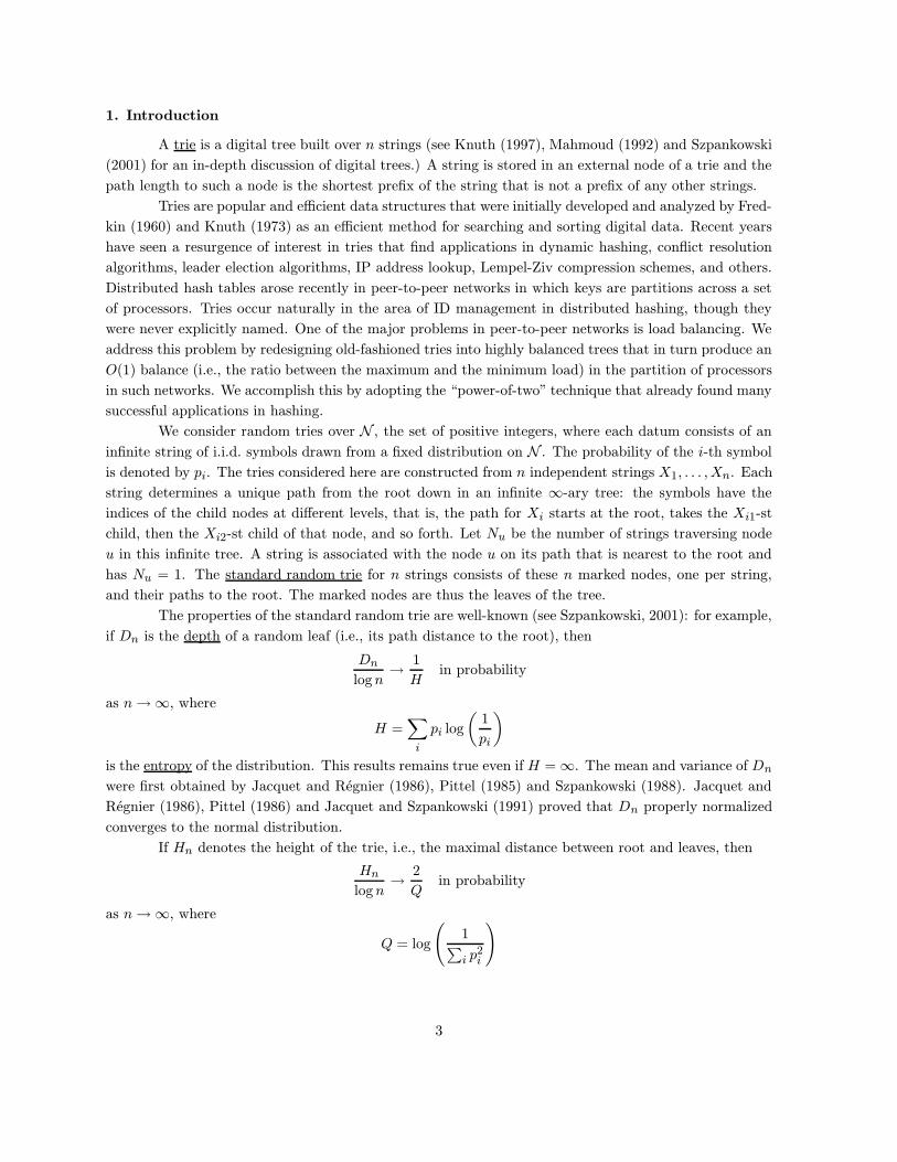
The properties of the standard random trie are well-known (see Szpankowski, 2001): for example,
if Dn is the depth of a random leaf (i.e., its path distance to the root), then
Dnlogn
→ 1
Hin probability
as n→∞, where
H =∑
i
pi log
(1
pi
)
is the entropy of the distribution. This results remains true even if H =∞. The mean and variance of Dn
were first obtained by Jacquet and Regnier (1986), Pittel (1985) and Szpankowski (1988). Jacquet and
Regnier (1986), Pittel (1986) and Jacquet and Szpankowski (1991) proved that Dn properly normalized
converges to the normal distribution.
If Hn denotes the height of the trie, i.e., the maximal distance between root and leaves, then
Hnlogn
→ 2
Qin probability
as n→∞, where
Q = log
(1∑i p
2i
)
3

(Pittel, 1985). From Jensen’s inequality and (maxi pi)2 ≤∑i p
2i ≤ maxi pi, we have
1
H≤ 1
Q≤ 1
log(
1maxi≥1 pi)
) ≤ 2
Q,
so that the height is always at least twice as big as the typical depth of a node.
In some applications, it is important to reduce the height as much as possible. Attempts in
this direction include patricia trees (Morrison, 1968) and digital search trees (Coffman and Eve, 1970,
Konheim and Newman, 1973). In patricia trees, all internal nodes with one child are eliminated. In
digital search trees, each internal node is associated with a string, namely the first string that visits that
node (the order of X1, . . . , Xn thus matters). In both cases, we have
Hnlogn
→ 1
log(
1maxi≥1 pi)
) in probability
(Pittel, 1985). In other words, the height of the latter variants of tries improves over that of the random
trie, but by not more than 50%. Also, both patricia trees and digital search trees introduce slight
inconveniences: “in order traversal” of digital search trees does not visit the nodes in sorted order, and
internal edges of patricia trees have cumbersome labels.
In the so called b-tries, one allows to store in an external node up to b strings (i.e., there are at
most b strings sharing the same prefix). For such a b-trie,
Hnlogn
→ b+ 1
log
(1∑
i pb+1i
) in probability
(Pittel (1985), see also Szpankowski, 2001).
The height is not the only balance parameter. In a trie with finite fanout β (i.e., Xi takes values
on {1, . . . , b}), the fill-up level Fn, the distance from the root to the last level that has a full set of βFn
nodes, is also important. Pittel (1986) found the typical value of the Fn in a trie built over n strings
generated by mixing sources. For memoryless sources,
Fnlogn
→ 1
log(1/pmin)=
1
h−∞in probability
where pmin = mini{pi} is the smallest probability of generating a symbol and h−∞ = log(1/pmin) is
the Renyi entropy of infinite order (Szpankowski (2001)). This was further extended by Pittel (1986),
Devroye (1992), and Knessl and Szpankowski (2005) who proved that the fill-up level Fn is concentrated
on two points kn and kn + 1, where for asymmetric sources kn is an integer
1
log(1/pmin)(logn− log log logn) +O(1)
while for symmetric sources (i.e., sources with p1 = p2 = 1/2) kn is
log2 n− log2 log2 n+O(1).
Observe that in the symmetric case we have log logn instead of log log logn.
To understand why balanced tries are relevant to load balancing in peer-to-peer networks, consider
the following scenario discussed in Malkhi et al. (2002) and Adler et al. (2003). In peer-to-peer networks,
each of n processor is given a key which is mapped into the interval [0, 1]. Thus, processors can be
considered as infinite binary strings. These strings are organized as in a binary trie. When the keys are
4

uniform on [0, 1], then the bits are i.i.d. with p1 = p2 = 1/2, as in standard binary trie. The trie is used
to locate peers with close keys, and the table of keys is also called a distributed hash table.
There are a number of performance measures for distributed hash tables. Among them the search
time (the number of queries required to locate a requested item) and load balancing (how load is balanced
between the processors) are the most important. Since every processor is assigned to a subinterval in [0, 1]
(namely the one controlled or “owned” by its key, which could, but does not have to be at its center),
load balancing can be measured by the ratio Bn of the largest to the smallest assigned subinterval. The
goal is to design hash tables with bounded balance ratio.
We address load balancing and search time issues in the context of the associated tries. In order
to construct a well balanced trie needed for an efficient distributed hash table, we design a new trie in
which every processor has O(log n) keys to be tried before inserting into the trie the key that has the
smallest depth of insertion. We will argue that in a problem of ID management in peer-to-peer networks
the relevant quantity is the ratio
Bn = 2Hn−Fn ,
where Hn and Fn are the height and the fill-up level in the associated trie, respectively. In view of this
a well balanced network requires to design a well-balanced trie with Hn − Fn = O(1). As the first step
we propose the so called two-choice trie in which we deal with pairs of strings. A simple argument shows
that if, in an on-line fashion, for every pair of strings one inserts in the trie the one that has smaller depth
of insertion, then for symmetric sources
Hnlogn
→ 3
2Qin probability,
resulting in a 25% reduction in height compared to standard tries. However, even with such a reduction
in height, one has Hn − Fn = Θ(logn) in probability.
To reduce the height further, we design a refined version of the power-of-two tries in which one
selects n strings resulting in a height that is close to the smallest possible. Call this height H∗n. We design
an on-line algorithm with total computational time O(n log n) such that
H∗nlogn
→ 1
Qin probability.
Interestingly, one can further reduce the height by considering tries with k choices for large k.
We prove that if k is sufficiently large (but fixed) then the ratio H∗n/ logn approaches 1/H with arbitrary
precision, a bound that cannot be improved.
Finally, we consider tries with k choices for symmetric sources when k is allowed to grow with
n. In particular, we show that if the number of choices per datum is proportional to logn, then with
high probability a nearly perfectly balanced trie exists with Hn − Fn ≤ 2. Furthermore, we show that
by a natural greedy on-line algorithm one also achieves nearly perfect balancing with Hn − Fn ≤ 7 with
probability 1 − o(1). This has applications for load balancing in peer-to-peer networks. In particular,
the result implies that if in a peer-to-peer network in which ID’s of the n hosts are organized on a
circle and upon arrival, each host is allowed to try c logn randomly chosen ID’s and choose the one that
maximizes its distance from its neighbors then the maximal load balance ratio remains bounded with
high probability.
5

2. Two-choice tries.
In this section we consider the situation when each datum has two independent strings Xi and
Yi drawn from our string distribution, and that we are free for pick one of the two for inclusion in
the trie. Define Zi(0) = Xi, Zi(1) = Yi, let {i1, . . . , in} ⊆ {0, 1}n, and let Hn(i1, . . . , in) denote the
height of the trie for Z1(i1), . . . , Zn(in). Thus, with n data pairs, we have 2n possible random tries. Let
H∗n = mini1,...,in Hn(i1, . . . , in) be the minimal height over all these 2n tries.
The paradigm of two choices, applied here for tries, was successfully applied in hashing, see Azar,
Broder, Karlin and Upfal (1994, 1999), Czumaj and Stemann (1997) and Pagh and Rodler (2001).
We show the following:
Theorem 1. Assume that the vector of pi’s is nontrivial (maxi pi < 1). Then H∗n/ logn → 1/Q in
probability. In particular, for fixed t ∈ R,
P{H∗n ≥
logn + t
Q
}≤ 8e−t.
Also, for all ε > 0,
limn→∞P
{H∗n ≤
(1− ε) logn
Q
}= 0.
This theorem shows that the asymptotic improvement over standard random tries is 50%. Furthermore,
the height is less than or equal to the height of the corresponding patricia and digital search trees.
In Section 2.2, we deal with an efficient algorithm for constructing a good trie. The upper bound
in Theorem 1 will be shown to hold for Hn, the height of the trie obtained by a simple algorithm. Hence,
the algorithm is optimal to within a term that is o(logn) in probability. We stress that the results in
the entire section are for tries with an unlimited number of possible children. We start by constructing
a two-choice trie that achieves the upper bound of Theorem 1. This is followed by a description of an
O(n log n) on-line algorithm that realizes this trie. Finally, we prove the lower bound.
2.1 The upper bound.
In the infinite trie formed by all 2n strings, we consider all subtrees Tj , j ≥ 1 rooted at nodes
at distance d from the root. We sometimes write Tj(d) to make the dependence upon d explicit. More
often, we just use Tj . We say that a string visits Tj if the root of Tj is on the path of the string. Prune
this forest of trees by keeping only those that contain at least two leaves. Define
λ =∑
i
p2i .
The following lemma is immediate from the definition of the trie.
Lemma 1. A bad datum is one in which both of its strings fall in the same Tj . The probability that
there exists a bad datum anywhere is not more than
nλd.
We also need a lemma for pairs of data.
6

Lemma 2. A colliding pair of data is such that for some j 6= k, each datum in the pair delivers one string
to Tj and one string to Tk. The probability that there is a colliding pair of data anywhere is not more
than
2n2λ2d.
Proof. Fix a pair of data. The probability that the first strings in each datum fall in the same Tj is λd.
The probability that each datum puts its first string in Tj and second in Tk is thus not more than λ2d.
Summing over all pairs and combinations of collisions, we obtain the upper bound(n
2
)× 4× λ2d.
Next, we consider a multigraphG(d) (or just G), whose vertices represent the Tj(d)’s. We connect
Tj with T` if a datum deposits one string in each of these trees. With Tj we keep a list of indices of data
for which at least one of the two strings visits Tj .
1 2 3 3’ 2’ 1’
T1 T2 T3
d
T1
T3
T2
1
1’2’
3’
2
3
graph G
Figure 1. The multigraph G and an infinite trie for n = 3 pairsof strings, denoted by (1, 1′), (2, 2′) and (3, 3′). Note that (2, 2′)and (3, 3′) is a colliding pair.
Lemma 3. The probability that G has a cycle of length ≥ 3 is not more than
(4n)3λ3d
1− 4nλd.
7

Proof. The probability of a cycle of length ` can be bounded by the number of possible data assignments
times the probability that the ` pairs of data are in the given lists. This is not more than
2` (2n)` λd`.
Thus, the probability of a cycle of length ≥ 3 does not exceed
∞∑
`=3
(4n)`λd` =(4n)3λ3d
1− 4nλd.
So, finally, assuming that there is no bad datum, no colliding data and no cycle (so that G is a
forest with no multiedges), we can assign strings as follows. For each tree in turn pick any node as the
root. Then choose any one of the strings in the root node’s list. For all other strings in the root’s list,
choose the companion string of the same datum (found by following edges away from the root). This
either terminates, or has an impact on one or more child trees. But for the child tree of the root, we have
fixed one string (as we did for the root), and thus choose again companion strings for that child list, and
so forth. This process is continued until one string of each datum is chosen for the trie. In this manner,
the height Hn of the trie for the data selected by this procedure is not more than d. Therefore, we have
shown that
P{Hn > d} ≤ P{there exists a bad datum}+ P{there exists a colliding pair}+ P{there exists a cycle}
≤ nλd + 2n2λ2d +(4n)3λ3d
1− 4nλd.
If we set A = nλd, then
P{Hn > d} ≤ min
(A+ 2A2 +
64A3
1− 4A, 1
)≤ 4A1A≤1/8 + 1A>1/8 ≤ 4A1A≤1/8 + 8A1A>1/8 ≤ 8A.
We summarize:
Theorem 2. There exists a way of assigning the strings such that the trie satisfies, for all n and d,
P{Hn > d} ≤ 8nλd.
In particular,
P{Hn >
logn
Q+ t
}≤ 8e−t
for all n, t and vectors (p1, p2, . . .).
The proof above relates to our algorithm. It is noteworthy that the algorithm has a bit of slack,
because a choice of strings in the n data is only possible if and only if one of the connected components
in G has more than one cycle. With one cycle, it is still possible to pick the strings. However, it is not
worth the trouble to design a more complicated algorithm for a small gain in height. That limitation of
the gain in height is explained by the lower bound shown below.
8
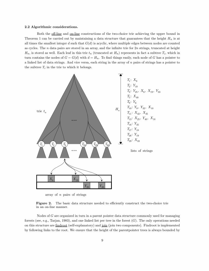
2.2 Algorithmic considerations.
Both the off-line and on-line constructions of the two-choice trie achieving the upper bound in
Theorem 1 can be carried out by maintaining a data structure that guarantees that the height Hn is at
all times the smallest integer d such that G(d) is acyclic, where multiple edges between nodes are counted
as cycles. The n data pairs are stored in an array, and the infinite trie for 2n strings, truncated at height
Hn, is stored as well. Each leaf in this trie tn (truncated at Hn) represents in fact a subtree Ti, which in
turn contains the nodes of G = G(d) with d = Hn. To find things easily, each node of G has a pointer to
a linked list of data strings. And vice versa, each string in the array of n pairs of strings has a pointer to
the subtree Ti in the trie to which it belongs.
T1 T2 T3 T28 T29 T30
...
...
Hn
X6 X19
Y25 Y33
trie tn
array of n pairs of strings
T1 : X9
T2 : Y10
T3 : Y25 , X6 , X19 , Y33
T5 : X40
T8 : Y6
T10 : Y9 , Y32 , X10
T11 : X32 , X35
T13 : X25 , Y40 , X18
T16 : Y35
T17 : Y18
T26 : Y19
T29 : X33
lists of strings
Figure 2. The basic data structure needed to efficiently construct the two-choice triein an on-line manner.
Nodes of G are organized in turn in a parent pointer data structure commonly used for managing
forests (see, e.g., Tarjan, 1983), and one linked list per tree in the forest (G). The only operations needed
on this structure are findroot (self-explanatory) and join (join two components). Findroot is implemented
by following links to the root. We ensure that the height of the parentpointer trees is always bounded by
9

log2 n, where n is the number of nodes in the tree. A join proceeds by making the root of the smallest
of the two subtrees the child of the root of the other tree. The two linked lists of the nodes in the trees
are joined as well. This takes constant time. By picking the smaller tree, we see that the height of the
parent pointer tree is never more than log2 n.
T3 T5 T8
T17 T26 T29
T16
T1
T10 T2
T13
T11
...
Figure 3. The forest G is maintained by organizing each tree component in aparentpointer tree. The components in the figure might correspond, for example, tothe list of strings given in the previous figure.
Assume that we have maintained this structure with n data pairs and that the height of tn is
h = Hn. Then, inserting data pair n + 1, say (X,Y ), into the structure proceeds as follows: for X and
Y in turn, determine the nodes of G in which they live, by following paths down from the root in tn.
Let these nodes of G be Tj and Tk. Run findroot on both nodes, to determine if they live in the same
component. If they do not, then join the components of Tj and Tk, add X to the linked list of Tj , and
add Y to the linked list of Tk. The work done thus far is O(h+ logn).
If Tj and Tk are in the same component, then adding an edge between them would create a cycle
in G. Thus, we destroy tn and create t′n of height h+ 1 from scratch in time O(n) (see below how). An
attempt is made to insert (X,Y ) in t′n. We repeat these attempts, always increasing h by one, until we
are successful. The time spent here is O(n∆h), where ∆h is the number of attempts.
In a global manner, starting from an empty tree, we see that to create this structure of size n
takes time bounded by O(nHn + n logn). By Theorem 2, E{Hn} = O(log n). Therefore, the expected
time is O(n logn), which cannot be improved upon.
The space used up is O(nHn). It is known that for standard tries the expected number of
internal nodes is O(n/H), where H is the entropy (Regnier and Jacquet, 1989). While it is still true that
the expected number of internal nodes in the final trie is O(n) (because it is smaller than that for the
trie constructed using all 2n data strings), the intermediate structure needed during the construction is
possibly of expected size of the order of n logn.
Two details remain to be decided. First, we have to choose one element in each data pair. This
can be done quite simply by considering the roots for all components in turn. From the root tree in a
component, say Tr, pick any of its member strings, and assign it. Then traverse the component of Tr by
depth first search, where the edges are the edges of G (an edge of G is easily determined from the list of
10
strings in Tr, as each string points back to the tree Ti to which it belongs). At each new node visited,
if possible, pick the first string whose sibling has not been assigned yet. This process cannot get stuck
as there is no cycle in G, and it takes time O(n). In Figures 2 and 3, the component whose root tree is
T13 is traversed in this order: T13, T3, T8, T26, T29, T5 and T17. The string assignments for the six string
pairs in that 7-node component are, in order of assignment, X25, X6, Y6, Y19, X33, X40 and Y18. After the
assignment of all strings, it is a trivial matter to construct the final trie in time O(nHn).
The second detail concerns the extension of G and the necessary data structures when the height
h is increased by one. Here we first update the trie by splitting all the trees Tj appropriately. Create the
connected components by depth first search following the edges of G. This takes time O(n). Set up the
parent pointer data structure for each component of G by picking a root arbitrarily and making all other
nodes children of the root.
The discussion above ensures that we can construct the two-choice trie incrementally in O(n log n)
expected time. Also, in a dynamic setting, if the data structure defined above is maintained, then an
insertion can be performed in O(log n) expected amortized time, under the assumptions of the theorems
in this paper.
11
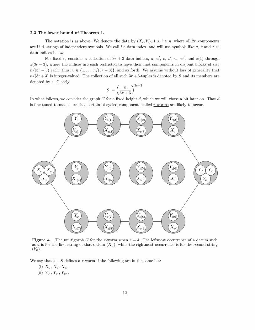
2.3 The lower bound of Theorem 1.
The notation is as above. We denote the data by (Xi, Yi), 1 ≤ i ≤ n, where all 2n components
are i.i.d. strings of independent symbols. We call i a data index, and will use symbols like u, v and z as
data indices below.
For fixed r, consider a collection of 3r + 3 data indices, u, u′, v, v′, w, w′, and z(1) through
z(3r − 3), where the indices are each restricted to have their first components in disjoint blocks of size
n/(3r + 3) each: thus, u ∈ {1, . . . , n/(3r + 3)}, and so forth. We assume without loss of generality that
n/(3r+ 3) is integer-valued. The collection of all such 3r+ 3-tuples is denoted by S and its members are
denoted by s. Clearly,
|S| =(
n
3r + 3
)3r+3
.
In what follows, we consider the graph G for a fixed height d, which we will chose a bit later on. That d
is fine-tuned to make sure that certain bi-cycled components called r-worms are likely to occur.
XuXv
Xw
Yu’Yv’
Yw’
Yu
Xz(1)
Yz(1)
Xz(2)
Yz(2)
Xz(3)
Yz(3)
Xu’
Yv
Xz(4)
Yz(4)
Xz(5)
Yz(5)
Xz(6)
Yz(6)
Xv’
Yw
Xz(7)
Yz(7)
Xz(8)
Yz(8)
Xz(9)
Yz(9)
Xw’
Figure 4. The multigraph G for the r-worm when r = 4. The leftmost occurrence of a datum suchas u is for the first string of that datum (Xu), while the rightmost occurrence is for the second string(Yu).
We say that s ∈ S defines a r-worm if the following are in the same list:
(i) Xu, Xv, Xw.
(ii) Yu′ , Yv′ , Yw′ .
12
(iii) Yu and Xz(1); Yz(1) and Xz(2); Yz(2) and Xz(3); . . .; Yz(r−1) and Xu′ . This defines a chain of r−1
lists of size two.
(iv) Yv and Xz(r); Yz(r) and Xz(r+1); Yz(r+1) and Xz(r+2); . . .; Yz(2r−2) and Xv′ . This defines a chain
of r − 1 lists of size two.
(v) Yw and Xz(2r−1); Yz(2r−1) and Xz(2r); Yz(2r) and Xz(2r+1); . . .; Yz(3r−3) and Xw′ . This defines
a chain of r − 1 lists of size two.
We have two lists of three, who by brotherhood are connected to each other by three chains of
lists of two. Observe that the r-worm refers to the subgraph of G induced by the 3r + 3 data indices
involved. If an r-worm exists, and we are forced to pick one string from each of the 3r + 3 data items,
then at least one of the lists in it must accept two strings, no matter how we assign the strings for the
indices represented in S (by the pigeon-hole principle, as the number of lists in the r-worm is 3r + 2).
Let N be the (random) number of r-worms. We thus have
P{H∗n ≤ d} ≤ P{N = 0}.We bound the right-hand side from above by the second moment method. Clearly,
E{N} = |S|λ3r2 λ
23,
where
λ`def=
(∑
i
p`i
)d.
We have the following inequalities, which are all consequences of Jensen’s inequality:
(∑
i
pqi
) 1q
↓
as q ↑ ∞, and
e−H ≤(∑
i
pqi
) 1q−1
↑
as 1 ≤ q ↑ ∞. The last expression is the so-called Renyi entropy of order q. Using λ23 ≥ λ4
2, we have
E{N} ≥ (nλ2)3r+4
n(3r + 3)3r+3.
It is convenient to use Zs for the indicator function that s ∈ S defines an r-worm. We write
s ∼ s′ when the data indices of s and s′ overlap and s 6= s′. Let δ(s, s′) be the number of positions in
which s and s′ agree (i.e., 3r + 3 minus the Hamming distance): 0 ≤ δ(s, s′) ≤ 3r + 3. Using V{·} to
denote the variance, we have
V{N} ≤∑
s
E{Zs}+∑
s∼s′E{ZsZs′} = E{N}+
∑
s∼s′E{ZsZs′}
For 0 ≤ ` ≤ 3r + 3, we have
∣∣{(s, s′) : δ(s, s′) = `}∣∣ =
(n
3r + 3
)3r+3
×(
n
3r + 3− 1
)3r+3−`×(
3r + 3
`
)≤ n6r+6−`
`!.
13

For s ∼ s′, set ` = δ(s, s′). In order to calculate the value of E{ZsZs′} for two given strings
s, s′ ∈ S, we must take into account the positions of those indices that agree in s and s′. (There are ` of
them.) We say that s and s′ define a joint r-worm if both s and s′ define r-worms (i.e., ZsZs′ = 1). Given
s, s′, consider the multigraph G for the joint r-worm (similar to Figure 2 but with s′ added). The size of
a node in this multigraph is defined as the number of strings corresponding to the node when s and s′
define a joint r-worm. For i = 2, 3, 4, 5, let ni be the number of nodes in the graph of size i. (Observe
that the sizes of the nodes vary from 2 to a maximum of 5.) Then clearly
E{ZsZs′} = λn22 λ
n33 λ
n44 λ
n55 ≤ λ
n22 λ
3n3+4n4+5n53
3 .
We will show below in Lemma 5 that we always have 3n3 + 4n4 + 5n5 ≥ 12 when ` ≤ r. For ` ≤ r,
E{ZsZs′} ≤ λn22 λ
3n3+4n4+5n5−123
3 λ43 ≤ λ
2n2+3n3+4n4+5n5−122
2 λ43 ≤ λ6r−`
2 λ43,
where we used λ1/33 ≤ λ1/2
2 and the fact that 2n2 + 3n3 + 4n4 + 5n5−12 = 12r−2` (see Lemma 4 below).
For ` > r, we simply have
E{ZsZs′} ≤ λn22 λ
3n3+4n4+5n53
3 ≤ λ2n2+3n3+4n4+5n5
22 = λ6r+6−`
2 .
By the second moment method Chung and Erdos (1952); see also Janson et al (2000)),
P{N = 0} ≤ V{N}V{N}+ (E{N})2 ≤
V{N}(E{N})2
≤ 1
E{N} +
∑s∼s′ E{ZsZs′}
(E{N})2
≤ 1
E{N} +3r+3∑
`=1
∑
s∼s′:δ(s,s′)=`max
s∼s′:δ(s,s′)=`E{ZsZs′}(E{N})2
≤ 1
E{N} +r∑
`=1
n6r+6−` λ6r−`2 λ4
3
`!(E{N})2+∑
`>r
(nλ2)6r+6−`
`!(E{N})2
def= I + II + III.
For fixed ε > 0, we set d = b(1− ε) logn/ log(1/λ)c and α = nλ2. Note that α = nλd ≥ nε →∞.
In particular, α ≥ 1 for all n ≥ 1. Take r so large that jointly ε(3r + 4) > 1 (so that E{N} → ∞ and
thus I = o(1)) and ε(r + 3) > 2 (needed below). Then
II ≤r∑
`=1
(3r + 3)6r+6
`! (nλ2)`≤ (3r + 3)6r+6
(e
1nλ2 − 1
).
Finally, using E{N} ≥ (nλ2)3r+4
n(3r+3)3r+3 ,
III ≤3r+3∑
`=r+1
(3r + 3)6r+6
`!λ22 (nλ2)`
≤3r+3∑
`=r+1
(3r + 3)6r+6n2
`! (nλ2)2+`≤ (3r + 3)6r+6en2
(r + 1)! (nλ2)r+3 .
14

If Cr denotes a constant depending upon r only, we see that
P{N = 0} ≤ Cr(nα−3r−4 + e1/α − 1 + n2α−r−3
)≤ Cr
(n−ε(3r+4) + en
−ε − 1 + n2−(r+3)ε)
= o(1).
That concludes the proof of the lower bound.
It remains to show the two structural properties of the joint r-worms defined by s and s′.
Lemma 4.
2n2 + 3n3 + 4n4 + 5n5 = 12r + 12− 2δ(s, s′).
Proof. The proof goes by induction. At the outset, we start with two disjoint r-worms so that n2 = 6r
and n3 = 4, and join one by one the δ(s, s′) entries of the r-worm defined by s′ that coincide with those
of s. One can verify that each such step makes 2n2 + 3n3 + 4n4 + 5n5 decrease by two. (For example, if
the u entry is processed first, then clusters of sizes 3, 3, 2 and 2 become clusters of sizes 5 and 3 in the
join.) Therefore, 2n2 + 3n3 + 4n4 + 5n5 = 12r + 12− 2δ(s, s′).
Lemma 5. For ` = δ(s, s′) ≤ r, we have 3n3 + 4n4 + 5n5 ≥ 12.
Proof. The proof is by contradiction. if 3n3 + 4n4 + 5n5 < 12, then n3 + n4 + n5 < 4, so at least
one border pair u, v, w, u′, v′, w′ must be identical. Let m3 be the number of clusters of size 3 that
involve non-border pairs. If m3 = 0, then that means that each row of r − 1 non-border indices (the
z’s) is either entirely identical or entirely different in s and s′. But if one such row is identical, then
` ≥ (r − 1) + 2 = r + 1. It is impossible to have all three rows non-identical, because then m3 would not
be zero. The case m3 ≥ 2 can be eliminated, as we would have n3 +n4 + n5 ≥ 2 +m+ 3 ≥ 4. So assume
m3 = 1. But then the clusters at the borders must both be hit at least once. For m3 = 1, this implies
that one row must necessarily be identical in s and s′, and one other row has its border pair in common
in s and s′. So, once again, ` ≥ r + 1.
2.4 A simple greedy heuristic
Instead of using the elaborate data structure described in Section 2.2 to construct the trie, we
could greedily pick one string according to a simple rule: choose the string which, at the time of its
insertion would yield the leaf nearest to the root. Once a selection is made, it is impossible to undo it at
a later time. This greedy heuristic yields a height that is guaranteed to be 25% better than that of the
ordinary trie (see Theorem 3 below), but it cannot achieve the 50% improvement of the main method
described in this paper (see Theorem 4 below). In this section, Hn refers to the height of the trie obtained
by this greedy heuristic.
Theorem 3. Assume the probabilistic model of Theorem 1. For all integer d > 0,
P {Hn ≥ d} ≤ 4n3e−2dQ + 2n2e−3dQ/2.
Thus, for any t > 0,
P{Hn ≥
3 logn+ t
2Q
}≤ 4e−t + 2n−1/4e−3t/4.
15

Proof. We consider once again the multigraph G = G(d) of Section 2.1, whose vertices represent the
Tj(d)’s. We connect Tj with T` if a datum deposits one string in each of these trees. Remove from this
graph all Tj ’s that have just one datum, and their incident edges. Call the remaining graph G′. We claim
that if Hn > d, then G′ has at least one edge. Indeed, assume the contrary. Then consider (Xi, Yi) at
time of processing by the algorithm. Let Xi share a prefix of length at least d with some strings Xj or
Yj for j < i (collected in a set Ai), Let Bi similarly be all strings Xj or Yj for j < i that share a prefix
of length d with Yi. By assumption, either Ai or Bi is empty. So, the greedy algorithm can pick Xi or
Yi so that no other previous string shares a prefix of length d or more. Let Ci denote the event that Xi
and Yi have a common prefix of length d. By negative association of the components of a multinomial
random variable,
P{Hn ≥ d} ≤n∑
i=1
P{min(|Ai|, |Bi|) ≥ 1}
≤n∑
i=1
(P2{|Ai| ≥ 1}+ P{Ci, |Ai| ≥ 1}
)
≤n∑
i=1
(2i− 2)2
(∑
`
p2`
)2d
+n∑
i=1
(2i− 2)
(∑
`
p3`
)d
≤ 4n3e−2dQ + 2n2e−3dQ/2.
The bound of Theorem 3 is tight in the finite equiprobable case p1 = · · · = pβ = 1/β, and thus
establishes the suboptimality of the greedy heuristic in that important special case. By continuity, the
suboptimality carries over to an open neighborhood of the equiprobable probability distribution (with
respect to the total variation metric).
Theorem 4. Assume the probabilistic model of Theorem 1, and that there exists an integer β such that
p1 = · · · = pβ = 1/β. Then, for all ε > 0,
limn→∞P
{Hn ≤
(3− ε) logn
2Q
}= 0.
Proof. Since all strings of length m have the same probability 1/βm, it is clear that if we randomize
the selection in case of a tie, then the events [Zi = Xi] (in the notation of the proof of Theorem 3) are
independent Bernoulli (1/2) random variables. Also, 1Zi=Xi is independent of Xi. Let S be the set of
indices for which Zi = Xi. For fixed t, we call a triple of indices (` > i > j) good if i, j ∈ S, and if
L(X`, Xi) ≥ t and L(Y`, Xj) ≥ t, where L(., .) is the lenghth of the common prefix of the two argument
strings. If a good triple exists, then Hn ≥ t. The expected number of good triples (N) is
(n
3
)1
4
(∑
i
p2i
)2t
∼ n3e−2tQ
24.
This tends to infinity if we take t ∼ 3(1 − ε) logn/(2Q) for ε > 0. It is a routine matter to apply the
second moment method to establish that in that case, P{N > 0} → 1. We sketch the proof. It suffices to
establish that V{N} = o((E{N})2). Simple case by case studies reveal that
V{N} = O(n5(λ2t
2 λt3 + λ2t
3
))+O
(n4(λt5 + λt2λ
t3 + λ2t
3
))
16

where λ`def=∑i p`i . Using the fact that in the equiprobable case, λ` = λ`−1
2 , we have V{N} =
O(n5λ4t
2 + n4λ3t2
), and this is easily seen to be (E{N})2×φn, where φn = O(1/n+1/(n2λt2)) = o(1/
√n).
Remark 1. If we perform the greedy heuristic with k choices, then an easy extension of the proof of
Theorem 4 shows that for fixed t > 0,
P{Hn ≥
(k + 1) logn+ t
kQ
}≤ kke−t + o(1).
3. Multiple choice tries.
3.1 The entropy lower bound.
If we have k choices per datum, then the height can be further reduced. However, in any case,
we cannot go beyond the entropy bound, as we will prove in this section. Recall that for an ordinary
trie, Dn = o(log n) in probability when H = ∞. We will not deal with those cases here. Let k ≥ 2 be a
fixed integer. Consider n data, each composed of k independent strings of i.i.d. symbols drawn from any
distribution on N . Let H∗n(k) denote the minimal height of any trie of n strings that takes one string of
each datum. We have the following lower bound:
Theorem 5. If the vector of pi’s is nontrivial (maxi pi < 1) and H < ∞, then for all k ≥ 2 and for all
ε > 0,
limn→∞P
{H∗n(k) ≤ (1− ε) logn
H
}= 0.
Proof. We fix d = b(1− ε) logn/Hc, and consider the partition of space defined by all different prefixes
of length d. There is an obvious analogy with cells or buckets. Partition the space of all strings into
buckets, where each bucket corresponds uniquely to a string of length d. We say that a string falls in
a given bucket if its length d prefix coincides with that for the bucket. Consider the kn strings, k per
datum, and let Mn denote the number of occupied buckets. It is clear that
[H∗n(k) ≤ d] ⊆ [Mn ≥ n].
Thus, it suffices to show that
limn→∞P{Mn ≥ n} = 0.
From an extension of Talagrand’s inequality (see, e.g., Boucheron, Lugosi and Massart (2000,
2003) or Devroye (2002)),
P{Mn ≥ E{Mn}+ t} ≤ exp
(− t2
2E{Mn}+ 2t/3
), t ≥ 0 .
Taking t = n/2, we are thus done if we can show that E{Mn} = o(n).
17
Let S be the (infinite) set of buckets in our collection, and for s ∈ S, define p(s) = P{X ∈ s},where X is a length d string consisting of i.i.d. symbols Y1, . . . , Yd drawn from {pi}. Define
Z =d∏
i=1
pYi .
Note that for fixed constant δ > 0,
|{s : knp(s) ≥ 1/δ}| ≤∑
s∈Sδknp(s) = δkn,
where we used Markov’s inequality. Thus
E{Mn} =∑
s∈S
(1− (1− p(s))kn
)
≤∑
s∈S:knp(s)≤1/δ
knp(s) + δkn
≤ knP{Z ≤ 1
δkn
}+ δkn
= knP
{d∑
i=1
log(1/pXi) ≥ log(δkn)
}+ δkn
= o(kn) + δkn,
where we used the law of large numbers, as E{log(1/pY1)} = H , and thus
∑di=1 log(1/pYi)
dH→ 1
in probability. Since δ > 0 was arbitrary, we have E{Mn} = o(n).
3.2 The entropy upper bound.
The bound of Theorem 5 is tight in the following sense:
Theorem 6. Assume H < ∞. In the notation of Theorem 5, we have for all ε > 0, there exists k large
enough such that
limn→∞P
{H∗n(k) ≥ (1 + ε) logn
H
}= 0.
Proof. Fix ε > 0 and k. Consider the trie formed by the kn input strings. For the j-th string of the i-th
datum, let Di,j be the maximal common prefix length with any string belonging to a datum not equal to
i (the other strings for datum i are thus ignored). Note that H∗n(k) ≤ maxi minj Di,j . It suffices to show
that
P{
maxi
minjDi,j ≥
(1 + ε) logn
H
}= o(1),
which is implied by
P{
minjD1,j ≥
(1 + ε) logn
H
}= o
(1
n
).
18

Let
d =
⌈(1 + ε) logn
H
⌉.
Let s1, . . . , sk be the strings of length d corresponding to datum 1 (note that duplicates are allowed), and
let N1, . . . , Nk be the number of strings among the remaining (n−1)k strings whose length d prefix agree
with s1, . . . , sk, respectively. Then
P{
minjD1,j ≥ d
}= P {N1 > 0, . . . , Nk > 0} .
Let A be the event that the cardinality C = |{s1, . . . , sk}| is ≤ k/2, where we assume k to be even. Set
θ = max` p`. We have
P{A} ≤(k
k/2
)((k/2)θd)k/2 = o(1/n)
by choice of k. We use the notation a1 6= a2 6= · · · 6= ak to denote the event that a1, a2, . . . , ak are all
different. Let B be the event [s1 6= · · · 6= sk/2]. We have P{Bc} ≤(k/2
2
)θd = o(1). Given s1 6= · · · 6= sk,
the Ni’s are part of multinomial random vector and thus negatively associated (Mallows, 1968). Therefore,
if S denotes the number of different values occurring among the si’s, and a1, . . . , aS are the indices of the
first occurrences of these S values, in order of occurrence among s1, . . . , sk,
P {N1 > 0, . . . , Nk > 0} = E {P {N1 > 0, . . . , Nk > 0|s1, . . . , sk}}≤ P{A}+ E {1Ac P {N1 > 0, . . . , Nk > 0|s1, . . . , sk}}
≤ P{A}+ E
{1Ac
S∏
i=1
P{Nai > 0|sai
}}
(by negative association of multinomial random variables)
≤ P{A}+ E
1Ac
k/2∏
i=1
P{Nai > 0|sai
}
≤ P{A}+ P{Ac}E
k/2∏
i=1
P{Nai > 0|sai
}|Ac
= P{A}+ P{Ac}E
k/2∏
i=1
P {Ni > 0|si} |s1 6= · · · 6= sk/2
≤ P{A}+P{Ac}E
{∏k/2i=1 P {Ni > 0|si}
}
P{s1 6= · · · 6= sk/2}
= P{A}+ (1 + o(1)) E
k/2∏
i=1
P {Ni > 0|si}
= P{A}+ (1 + o(1))
k/2∏
i=1
P {Ni > 0}
(by independence of the si’s)
= P{A}+ (1 + o(1)) (P {Ni > 0})k/2 .
19

Let Z1, . . . , Zd be the symbols occurring in s1. Then
P {N1 > 0} = E
1−
(1−
d∏
i=1
pZi
)(n−1)k
≤ E{
1−(
1− rd)(n−1)k
}+ P
{d∏
i=1
pZi > rd
}
≤ nkrd + P
{d∑
i=1
log(1/pZi) < d log(1/r)
}
= nkrd + exp (−d(o(1) + φ(log(1/r)))
as d → ∞ and r ∈ (0, 1) remains fixed, by Cramer’s large deviation theorem (see, e.g., Dembo and
Zeitouni, 1998). The function φ(u) is positive for all u < E{log(1/pZ1)} = H . Thus, for all fixed
1 > r > e−H , there exists a constant δ = δ(r) ∈ [0, 1) such that for all d,
P {N1 > 0} ≤ nkrd + δd.
Observe that if we set r = exp(−(1 + ε/2)H/(1 + ε)), then nrd ≤ n−ε/2. Combining all our bounds, we
see that
P{
minjD1,j ≥ d
}≤ o(1/n) + (1 + o(1))
(kn−ε/2 + δd
)k/2= o(1/n) +O
(n−kε/4 + δdk/2
)= o(1/n)
by choice of k.
Remark 2. One might ask for the exact constant in the weak limit of H∗n(k)/ logn. For k = 2, it is
1/Q as we showed earlier. However, for k > 2, the precise constant is harder to determine. The proof of
Theorem 6, suitably extended, yields the following upper bound for k fixed. Assume a finite entropy of
second order: H2def=∑i pi log2 pi <∞. Then, for all η > 0, and all k > k∗(η),
limn→∞P
{H∗n(k) ≥ (1 + (1 + η)ψ(k)) logn
H
}= 0,
where
ψ(k) = max
(4
k,
4√k
√H2 −H2
H
).
A brief sketch follows. It suffices to verify for which ε the last estimate in the proof of Theorem 6 is
o(1/n). Trivially, ε > 4/k is needed to make the first term o(1/n). So, let us verify under what condition
the last term is o(1/n). In other words, with the given choice of r, when is
P
{d∑
i=1
log(1/pZi) < d log(1/r)
}= o
(n−2/k
)?
Under the condition H2 <∞, we can easily verify from Taylor’s series with remainder that, as t ↓ 0,
log
(∑
i
pt+1i
)= −tH + (t2/2)(H2 −H2) + o(t2).
20

By Chernoff’s bound, for t > 0,
P
{d∑
i=1
log(1/pZi) < d log(1/r)
}≤ r−td
(∑
i
pt+1i
)d
= exp(−d(t log r + tH − (t2/2)(H2 −H2) + o(t2)
))
= exp
(−d(
(H + log r)2
2(H2 −H2)+ o(t2)
))
(upon putting t = (H + log r)/(H2 −H2) = H(ε/2)/(1 + ε)(H2 −H2))
= exp
(−d(
H2(ε/2)2
2(1 + ε)2(H2 −H2)+ o(ε2)
))(as ε ↓ 0)
≤ n− H(ε/2)2
2(1+ε)(H2−H2)+o(ε2)
= n− H(ε/2)2
2(H2−H2)+o(ε2)
.
The statement follows ifH(ε/2)2
2(H2 −H2)>
2
k.
In other words,
ε2 >16(H2 −H2)
kH.
21

4. Distributed hash tables and ID management.
Tries occur naturally, but not under the name “trie”, in the area of ID management in distributed
hash tables. In this area of network research, n hosts are assigned one ID in the unit interval [0, 1). The
unit interval is wrapped around to form a ring. At any time, the set of ID’s partition [0, 1) into n intervals
on the ring. The hosts are organized in the ring, linking to the next smaller and next larger host, and are
in general quite unaware of the ID’s of the other hosts, except what can be gleaned from traversing the
ring in either direction. Hosts are added and deleted in some way, but ID choices are up to the system.
Each interval is “owned” by the host to its left. Two parameters are of some importance here. The first
one is the balance Bn in the partition, as determined by the ratio of the lengths of the largest to the
smallest interval. Secondly, one must be able to determine quickly which host owns an interval in which
a given ID x falls. The latter is the equivalent of a search operation. Other complexity parameters for
updates are also important, but we will limit the discussion to Bn and the maximal search time.
interval ownedby ID
ID
(a)
interval ownedby ID
ID
(b)
Figure 5. Two ways of partitioning the space. In both (a) and (b), IDs are randomly generatedon the perimeter. In (a), IDs own the intervals to their left in clockwise order. In (b), IDs own aninterval whose boundaries are determined in some manner, e.g., by virtue of a trie or digital searchtree. A downloader or user generates a random number X on the perimeter and picks the owner ofthe interval of X for its job. The objective is to make all intervals of about equal length, so that allhosts receive about equal traffic.
ID’s are represented by their (infinite) binary expansions. Assume, for example, that the n ID’s
are i.i.d. and uniformly distributed on [0, 1). See, e.g., Ratnasamy et al (2001), Malkhi et al (2002)
or Manku et al (2003). Then it is a routine exercise in probability to show that the largest spacing
defined by the ID’s is asymptotic to logn/n in probability and that the smallest spacing is Θ(1/n2) in
probability (see Levy (1939) or Pyke (1965)). Thus, Bn is asymptotic to n logn in probability. Adler et
al (2003) and Naor and Wieder (2003) implicitly suggest a digital search tree approach. Consider first a
trie approach (not considered in those papers): the ID’s are considered as strings in a binary trie (with
p1 = p2 = 1/2), and ID’s are inserted sequentially as in a digital search tree. The binary expansions of
the nodes that are associated with the ID’s are the actual ID’s used (so, each ID is mapped to another
one). In the case of a trie, each leaf is associated with an ID. In the case of a digital serarch tree, each
internal node is mapped to an ID. That means that the ID’s used have only a finite number of ones in
their expansions. If the height of the trie is Hn, and the fill-up level (the number of full levels in the trie)
is Fn, then Bn = 2Hn−Fn+O(1). It is known that Hn = 2 log2 n+ O(1) in probability (Pittel, 1985) and
that Fn = log2 n − log2 log2 n + O(1) in probability, so that Bn = Θ(n logn) in probability. However,
22

for a digital search tree, we have Hn = log2 n + O(1) in probability, while Fn is basically as for tries.
Thus, Bn = O(log n) in probability. This is essentially the result Adler et al (2003) and Naor and Wieder
(2003) were after.
In an attempt to improve this, Dabek et al (2001) proposed attaching b = logn randomly
generated ID’s to each host, swamping the interval, and then making the ID assignments to guarantee
that Bn = O(1) in probability. However, some discard this solution as too expensive in terms of resources
for maintenance.
Abraham et al (2003), Karger and Ruhl (2003) and Naor and Wieder (2003) achieve Bn = O(1)
in probability while restricting hosts to one ID. In another approach, Abraham et al (2003) and Naor and
Wieder (2003) pick logn i.i.d. uniform random numbers per host, and assign an ID based on the largest
interval these fall into: the largest interval is split in half. A little thought shows that this corresponds
to a digital search tree in which logn independent strings are considered, and only one is selected for
insertion, namely the one that would yield a leaf nearest to the root. The fact that both Hn and Fn are
now log2 n+O(1) in probability yields the result.
Manku (2004) proposed a digital search tree with perfect balancing of all subtrees of size log2 n
(or something virtually equivalent to that). It also has Bn = O(1) in probability. A similar (but different)
view can also be taken for the trie version: start with an ordinary binary trie with the modification (see,
e.g., Pittel, 1985) that leaf nodes are mapped to their highest ancestors that have subtrees with b = log2 n
or fewer leaves. These ancestors are the leaves of the so-called ancestor trie. Construct such a binary
b-trie and its ancestor trie from n i.i.d. uniform [0, 1) random numbers. Now, for each ancestor, partition
its interval equally by spreading the leaves in its subtree out evenly when associating ID’s. We know
from the Erdos-Renyi law of large numbers that the maximal k-spacing (with k = c logn) determined by
n i.i.d. uniform [0, 1) random numbers is Θ(logn/n) in probability (Erdos and Renyi, 1970; Deheuvels,
1985; see also Novak, 1995). This would imply that all ancestors are at level log2 n− log2 log2 n+ O(1)
in probability, and that all intervals owned by the ID’s are Θ(1/n) in probability, from which Bn = O(1)
in probability.
The power-of-two choices can be explored in the present context. If we make an ordinary trie by
taking the best of two ID’s as described in this paper, and then map ID’s to the strings that correspond
to the corresponding leaf values, then Hn = log2 n + O(1) in probability. However, it is easy to verify
that Fn is as for the standard binary trie, so that Bn = O(log n) in probability. Indeed, the largest gap
defined by 2n uniform strings on [0, 1] is still Θ(logn/n) in probability.
However, the trick suggested by Abraham et al. (2003) and Naor and Wieder (2003) may make
Hn − Fn ≤ 2 with probability tending to one. However, we have two modifications: first, we insist on
using tries instead of digital search trees; and secondly, because of the use of tries, we have to modify the
selection heuristic as picking the largest interval is not good enough for tries. The next section contains
details of the construction of a trie that has both small height and large fill-up level, i.e., a trie that is
nearly perfectly balanced.
Finally a bibliographic remark. Tries have been explicitly used in several other ways for dis-
tributed hash tables. Balakrishnan et al (2003) use them in the Pastry network. Ramabhadran et
al. (2004) define a kind of trie called a prefix hash tree. More recent work on tries in this context was
done by Balakrishnan et al. (2005).
23

4.1 A well-balanced trie for ID management.
Consider the interval [0, 1] and let X1, . . . , Xn be n independent vectors of k = dc logne i.i.d.
uniform [0, 1] random variables Xi,j , 1 ≤ i ≤ n, 1 ≤ j ≤ k, where c > 0 is a constant. We first show that
we can pick X1,i1 , . . . , Xn,in such that the n spacings defined by these random variables on the circular
interval [0, 1] (the interval wrapped to a unit perimeter circle) are close to 1/n with high probability.
Denote by Mn the maximal spacing defined by a given selection X1,Z1, . . . , Xn,Zn where Z1, . . . , Zn are
random indices defined in some manner. Let mn denote the minimal spacing.
Lemma 6. Let α ∈ (0, 1) be fixed. Let c ≥ 2/α. Then there exists a selection Z1, . . . , Zn such that
X1,Z1, . . . , Xn,Zn satisfies, for n ≥ 8,
P{
1− αn
< mn ≤Mn <1 + α
n
}≥ 1− 3
n.
Proof. Partition [0, 1] into n equal intervals Ii, 1 ≤ i ≤ n, and let Ji be an interval of length α/n
centered within Ii. If our selection is such that each Ji receives exactly one random variable from the
n selected, then (1 − α)/n < mn ≤ Mn < (1 + α)/n. Thus, we need only be concerned with the event
A that there exists a selection vector that guarantees that each Ji is occupied. We use Hall’s theorem
(1935) (see also Bondy and Murty, 1976). We recall that in a bipartite graph with independent sets A
and B, there exists a perfect matching of all elements of A to different elements of B if and only if for
all sets S ⊆ A, |N(S)| ≥ |S|, where N(S) is the neighborhood of S in B. Consider a bipartite graph in
which the Xi’s form one part and the Jj ’s form the other part. For each Xi,` ∈ Jj , draw an edge from
Xi to Jj . Let Ni be the outdegree of Xi, a binomial (dc logne, α) random variable. By Hall’s theorem,
there does not exist a perfect matching between Xi’s and Jj ’s if and only if for some `, there exists a set
of ` Xi’s that have all their edges end up in a set S with |S| < `. By the union bound and conditioning
on the Ni’s,
P{Ac} = E {P{Ac|N1, . . . , Nn}} ≤ E
{n∑
`=1
(n
`
)(n
`− 1
)(`− 1
n
)N1+···+Nn}.
For a binomial (`, p) random variable B, we have E{sB} = (1 − p + ps)` ≤ exp(−p(1 − s)`), s ∈ (0, 1).
Thus, using the fact that N1 + · · ·+Nn is binomial (ndc logne, α),
E
n/2∑
`=1
(n
`
)(n
`− 1
)(`− 1
n
)N1+···+Nn ≤ 4ne−
αcn logn2 ≤
(4
n
)n≤ 1
n, n ≥ 8.
Also,
E
n∑
`=n/2
(n
`
)(n
`− 1
)(`− 1
n
)N1+···+Nn =
n/2∑
`=0
(n
`
)(n
`+ 1
)E
{(1− `+ 1
n
)N1+···+Nn}
≤n/2∑
`=0
n2`+1
`!(`+ 1)!
(1− α(`+ 1)
n
)cn log n
≤∞∑
`=0
n2`+1
`!(`+ 1)!e−αc(`+1) logn
24

≤ n1−αc∞∑
`=0
n`(2−αc)
`!(`+ 1)!
≤ 1
n
∞∑
`=0
1
`!(`+ 1)!
≤ 2
n.
Taken together, we have P{Ac} ≤ 3/n.
Theorem 7. Let α ∈ (0, 1/3) be fixed. Let c = 2/α. Then there exists a selection Z1, . . . , Zn such that
the height Hn and fillup level Fn of the associated trie for X1,Z1, . . . , Xn,Zn satisfy, for n ≥ 8,
P{Hn − Fn ≤ 2} ≥ 1− 3
n.
Proof. Consider the binary trie formed by the selection X1,Z1, . . . , Xn,Zn of Lemma 6. If a potential
node at distance d from the root is not realized, then there is a leaf at distance less than d from the
root. If that leaf is at distance d − 1, then only one string in the selection falls in the corresponding
interval, which has width 1/2d−1. Thus, the maximal spacing in the selection is at least half that, or
1/2d. Therefore, 1/2d ≤ Mn. Let Fn be the fill-up level, the distance to the last full level of nodes. We
have Fn = d− 1 if d is the first level with a missing node. Therefore
Fn ≥ log2(1/Mn)− 1.
On the other hand, Hn = h, then at distance h− 1, two strings in the selection visit the same node, and
thus, two strings are at distance less than 1/2h− 1 from each other. Thus, mn ≤ 1/2h−1, or
Hn ≤ log2(1/mn) + 1.
If the selection is such that (1− α)/n < mn ≤Mn < (1 + α)/n, then we have
dlog2 n− log2(1 + α)e − 1 ≤ Fn ≤ Hn ≤ blog2 n− log2(1− α)c+ 1.
We conclude
Hn − Fn ≤ 2 +
⌊log2
(1 + α
1− α
)⌋.
If α < 1/3, and c = 2/α, then the upper bound is 2.
25

4.2 An on-line algorithm for super-balancing.
Theorem 7 is an existence theorem, and is appealing since we did not even have to move or
transform any of the IDs. Recall that most ID management algorithms (e.g., Manku (2004)) allow hosts
to shift their ID’s to obtain a better partition. The actual construction may be cumbersome, though.
We have not established an algorithm, even for b = 2, that can achieve such a balance on-line while not
sending many messages in the network.
So, let us find an on-line algorithm that achieves the super-balancing predicted by Theorem 7.
Only, the spacings referred to in the definition of Bn now refer to the ID’s mapped to the leftmost parts
of the intervals in the trie (see below). For each of n hosts, k = dc logne i.i.d. uniform [0, 1] potential
ID’s are generated, Ui(1), . . . , Ui(k), 1 ≤ i ≤ n. We build an ordinary trie Tn for the binary expansions
of U1(Z1), . . . , Un(Zn), where the Zi’s are the selections. To define Zn+1, consider the tries Tn,j for Tnwith Un+1(j) added, 1 ≤ j ≤ k. This is easily done by trying to insert each ID separately. If Dn+1(j) is
the depth of the leaf of Un+1(j) after insertion into Tn, then
Zn+1 = arg minDn+1(j),
where ties are broken randomly. In other words, we pick the ID that at the moment of its birth has the
shortest distance to the root of the trie. The actual ID assigned is implicit in the path to the root: it has
a common prefix with (the binary expansion of) Un+1(j). This scheme generalizes the best of two-strings
greedy algorithm studied earlier in the paper. Unlike with two choices, with k = c logn choices one does
not lose optimality by a greedy construction. We first consider the height Hn.
internal nodeexternal nodeleaf
0 1
Figure 6. A standard trie for five strings. The correspondence between nodes and intervals in a dyadicpartition of the unit interval is shown. The leaf ID assigned is read from the path to the root (0 for left, 1for right). The external nodes, not normally part of the trie, are shown as well. Together, external nodes andleaves define a partition of the unit interval (shaded boxes). The fill-up level of this tree is one, while the heightis four.
Theorem 8. Let c > 1/ log 2 and k = dc logne in the greedy heuristic for assigning IDs. Then
P{Hn ≥ log2 n+ 3} ≤ n1−c log 2.
26

Proof. Given that Hn−1 < h, we have Hn ≥ h if and only if Un(Zn) lands within 1/2h−1 of one of
U1(Z1), . . . , Un−1(Zn−1). The probability of this is conservatively bounded by
(2(n− 1)
2h−1
)k,
for if one Un(j) is further than 1/2h−1 away from each U1(Z1), . . . , Un−1(Zn−1), it will result in a leaf
that is less than distance h away from the root. Thus, with h = dlog2 n+ 3e,
P {Hn ≥ h} ≤n∑
i=1
P {Hi ≥ h|Hi−1 < h} ≤ n(
1
2
)k≤ n1−c log 2.
It is a bit harder to deal with the fill-up level, Fn.
Theorem 9. Let c > (8/5) log 2 and k = dc logne in the greedy heuristic for assigning IDs. Then
P{Fn ≤ log2 n− 4} = O(1/ log2 n).
Proof. We consider vertices (and intervals) in the infinite binary tree level by level, where level refers
to distance from the root. Level h thus has 2h vertices (intervals). We consider two sets of vertices in
the trie, leaves (the set is denoted by L), and external nodes that are child nodes of non-leaf nodes in the
trie (the set is denoted by E). The nodes E are thus not part of the trie. The intervals that the nodes in
L and E together represent form a partition of [0, 1]. When a string is inserted in the trie, it visits only
one of these intervals. If it belongs to E, then that node in E joins L, and the string is associated with
that new leaf. If it belongs to L, then the string occupying that leaf and the new string find the first
bit on which they disagree. If this is bit h, then the old leaf node is deleted, and two new leaf nodes are
created at level h. In addition, a number of new external nodes may have been created. In particular, if
that leaf interval hit by the new string is at level `, then h = ` + 1 with probability 1/2. Let th be the
first time that all nodes of E and L are at level h or higher. Let sh be the first time ≥ th such that all
nodes of E (if any) are at level strictly higher than h. If E is empty at time th, then sh = th. Let Fhdenote the σ-algebra generated by all Ui(j), i ≤ th. Let Gh denote the σ-algebra generated by all Ui(j),
i ≤ sh. We will find upper bounds for sh − th and th+1 − sh for all h, by bounding the time needed to
clear level h, first from leaves, and then from external nodes. In what follows, we will use the duality
P{Fn ≤ h} = P{sh > n}.To bound sh − th, we start with a number of external node intervals that is anywhere between 0
and 2h. Consider the worst scenario, where at time th, there are exactly 2` such nodes. The objective,
as in the coupon collector problem, is to hit each interval with a string. Given that there are ` external
nodes left, the probability of eliminating one of them by our greedy algorithm (when inserting one new
node) is
q`,hdef= 1−
(1− `
2h
)k.
If the waiting time until this happens is T`,h, then we have
P{T`,h ≥ t} = (1− q`,h)t−1 ≤ e1−q`,ht, t ≥ 1.
27

Thus, T`,h is stochastically dominated ((st)≤ ) by 1+Z`,h/q`,h, where Z`,h is an exponential random variable.
Thus, given Fh, and letting all Z’s in the sum below be i.i.d. exponential random variables,
sh − th(st)≤
2h∑
`=1
(1 +
Z`,hq`,h
)= 2h +
2h∑
`=1
Z`,hq`,h
.
Having cleared level h of all external nodes, we proceed to clear it from leaves. Note that a leaf
is eliminated if one of the leaf intervals gets hit in a way that would induce the creation of two leaves
at level h+ 1 (the conditional probability of this is 1/2). Arguing as for the external nodes, we see that
given ` leaf intervals, elimination happens with probability at least
p`,hdef= 1−
(1− `
2h+1
)k.
If the waiting time until this happens is T ′`,h, then we have
P{T ′`,h ≥ t} = (1− p`,h)t−1 ≤ e1−p`,ht, t ≥ 1.
Thus, T ′`,h is stochastically dominated by 1 + Z ′`,h/p`,h, where Z ′`,h is an exponential random variable.
Thus, given Gh, and letting all Z ′’s in the sum below be i.i.d. exponential random variables,
th+1 − sh(st)≤
2h∑
`=1
(1 +
Z ′`,hp`,h
)= 2h +
2h∑
`=1
Z ′`,hp`,h
.
We use duality. Setting s0 = 1, we have, using the above stochastic domination bounds, and
p`,h−1 = q`,h, a simple coupling argument shows that
h∑
r=1
(sr − tr + tr − sr−1)(st)≤
h∑
r=1
2r + 2r−1 +
2r∑
`=1
Z`,rq`,r
+2r−1∑
`=1
Z ′`,r−1
q`,r
,
and therefore
P{Fn ≤ h} = P{sh > n}
= P
{h∑
r=1
(sr − tr + tr − sr−1) > n− 1
}
≤ P
h∑
r=1
2r + 2r−1 +
2r∑
`=1
Z`,rq`,r
+2r−1∑
`=1
Z ′`,r−1
q`,r
> n− 1
≤ P
2h+1 + 2h − 3 + 2
h∑
r=1
2r∑
`=1
Z`,rq`,r
> n− 1
≤ P{
3× 2h +X > n+ 2}
≤ P{X − E{X} > n+ 2− 3× 2h − E{X}
}
≤ V{X}(n+ 2− 3× 2h − E{X}
)2 ,
28

by Chebyshev’s inequality, where all the Z’s above are i.i.d.,
X = 2h∑
r=1
2r∑
`=1
Z`,rq`,r
,
and we assume that n+ 2− 3× 2h − E{X} > 0.
E{X} = 2h∑
r=1
2r∑
`=1
1
q`,r,
and
V{X} = 4h∑
r=1
2r∑
`=1
1
q2`,r
.
We use the following lower bounds:
q`,hdef= 1−
(1− `
2h
)k≥ 1− e−k`/2h ≥ e− 1
e×min
(1,k`
2h
).
Thus,
E{X} = 2h∑
r=1
2r∑
`=1
1
q`,r
≤ 2h∑
r=1
∑
max(1,2r/k)≤`≤2r
1
q`,r+ 2
h∑
r=1
∑
1≤`≤2r/k
1
q`,r
≤h∑
r=1
2r+1e
e− 1+
2e
e− 1
h∑
r=1
∑
1≤`≤2r/k
2r
k`
≤ 2h+3 +2e
e− 1
h∑
r=1
2r(1 + r log(2))
k
≤ 2h+3 +2h+3(1 + h log(2))
k.
Similarly,
V{X} ≤ 4h∑
r=1
∑
max(1,2r/k)≤`≤2r
1
q2`,r
+ 4h∑
r=1
∑
1≤`≤2r/k
1
q2`,r
≤h∑
r=1
2r+2e2
(e− 1)2+
4e2
(e− 1)2
h∑
r=1
∑
1≤`≤2r/k
22r
k2`2
≤ 2h+5 +8λ2
3
h∑
r=1
22r
k2
≤ 2h+5 +22h+6
k2.
29

Putting everything together, we see that when h = blog2 n−Rc, R ∈ N , we have
P{Fn ≤ h} ≤2h+5 + 22h+6
k2(n+ 2− 3× 2h − 2h+3 − 2h+3(1+h log(2))
k
)2= O
(1
k2
)
if (3 + 8 + 8 log(2)/c)/2R < 1. We can always find such a c when R ≥ 4. In fact, for R = 4, it suffices to
set c > 8 log 2/5.
In conclusion, Hn − Fn ≤ 7 with probability tending to one when c > 1/ log 2. This implies
that Bn = O(1) in probability when spacings are defined with respect to leftmost points of leaf intervals.
Finally, the trie scheme proposed here assumes that one knows n, while in distributed networks, n is
unknown. However, one can estimate n by 2D, where D is the depth of insertion of a random string in
the trie: since all depths are within O(1) of log2 n, the estimate is off by a constant factor only. One can
thus extend the method in this manner by replacing k = c logn throughout by cD where D is the depth
of insertion of a random string.
References.
I. Abraham, B. Awerbuch, Y. Azar, Y. Bartal, D. Malkhi, and E. Pavlov, “A generic scheme for build-
ing overlay networks in adversarial scenarios,” in: Proceedings of the International Parallel and Dis-
tributed Processing Symposium (IPDPS 2003), 2003.
M. Adler, E. Halperin, R. M. Karp, and V. V. Vazirani, “A stochastic process on the hypercube with ap-
plications to peer-to-peer networks. ,” in: Proceedings of the 35th ACM Symposium on Theory of Com-
puting (STOC 2003), pp. 575–584, 2003.
Y. Azar, A. Z. Broder, A. R. Karlin, and E. Upfal, “Balanced allocations (extended abstract),” in: Pro-
ceedings of the 26th ACM Symposium on the Theory of Computing, pp. 593–602, 1994.
Y. Azar, A. Z. Broder, A. R. Karlin, and E. Upfal, “Balanced allocations,” SIAM Journal on Comput-
ing, vol. 29, pp. 180–200, 1999.
H. Balakrishnan, M. F. Kaashoek, D. Karger, R. Morris, and I. Stoica, “Looking up data in P2P sys-
tems,” Communications of the ACM, vol. 1946, pp. 43–48, 2003.
H. Balakrishnan, S. Shenker, and M. Walfish, “Peering peer-to-peer providers,” in: Peer-to-Peer Sys-
tems IV, 4th International Workshop, IPTPS 2005, Ithaca, NY, (edited by M. Castro, R. van Re-
nesse (eds)), vol. 3640, pp. 104–114, Lecture Notes in Computer Science, Springer-Verlag, 2005.
J. A. Bondy and U. S. R. Murty, Graph Theory with Applications, North-Holland, Amsterdam, 1976.
S. Boucheron, G. Lugosi, and P. Massart, “A sharp concentration inequality with applications in ran-
dom combinatorics and learning,” Random Structures and Algorithms, vol. 16, pp. 277–292, 2000.
S. Boucheron, G. Lugosi, and P. Massart, “Concentration inequalities using the entropy method,” An-
nals of Probability, vol. 31, pp. 1583–1614, 2003.
30

K. L. Chung and P. Erdos, “On the application of the Borel-Cantelli lemma,” Transactions of the Amer-
ican Mathematical Society, vol. 72, pp. 179–186, 1952.
E. G. Coffman and J. Eve, “File structures using hashing functions,” Communications of the ACM,
vol. 13, pp. 427–436, 1970.
I. Csiszar, “On generalized entropy,” Studia Scientiarium Mathematicarum Hungarica, vol. 4, pp. 401–
419, 1969.
A. Czumaj and V. Stemann, “Randomized Allocation Processes,” in: Proceedings of the 38th IEEE Sym-
posium on Foundations of Computer Science (FOCS’97), October 19-22, 1997, Miami Beach, FL, pp. 194–
203, 1997.
F. Dabek, M. F. Kaashoek, D. Karger, R. Morris, and I. Stoica, “Wide-area cooperative stor-
age with CFS,” in: Proceedings of the 18th ACM Symposium on Operating Systems Principles (SOSP
2001), pp. 202–215, 2001.
P. Deheuvels, “On the Erdos-Renyi theorem for random fields and sequences and its relation-
ships with the theory of runs and spacings,” Zeitschrift fur Wahrscheinlichkeitstheorie und verwandte Ge-
biete, vol. 70, pp. 91–115, 1985.
A. Dembo and O. Zeitouni, Large Deviations Techniques and Applications (Second Edition), Springer-
Verlag, New York, 1998.
L. Devroye, “Laws of large numbers and tail inequalities for random tries and Patricia trees,” Jour-
nal of Computational and Applied Mathematics, vol. 142, pp. 27–37, 2002.
P. Erdos and A. Renyi, “On a new law of large numbers,” J. Anal. Math., vol. 22, pp. 103–111, 1970.
E. H. Fredkin, “Trie memory,” Communications of the ACM, vol. 3, pp. 490–500, 1960.
P. Hall, “On representatives of subsets,” Journal of the London Mathematical Society, vol. 10, pp. 26–
30, 1935.
P. Jacquet and M. Regnier, “Trie partitioning process: limiting distributions,” in: CAAP 86, (edited
by P. Franchi-Zannettacci), vol. 214, pp. 196–210, Lecture Notes in Computer Science, Springer-Verlag,
Berlin, 1986.
S. Janson, T. Luczak, and A. Rucinski, Random Graphs, Wiley-Interscience, New York, 2000.
D. R. Karger and M. Ruhl, “New algorithms for load balancing in peer-to-peer systems,” IRIS Stu-
dent Workshop, 2003.
D. E. Knuth, The Art of Computer Programming, Vol. 3 : Sorting and Searching, Addison-Wesley, Read-
ing, Mass., 1973.
A. G. Konheim and D. J. Newman, “A note on growing binary trees,” Discrete Mathematics, vol. 4, pp. 57–
63, 1973.
P. Levy, “Sur la division d’un segment par des points choisis au hasard,” Comptes Rendus Acad. Sci .
Paris, vol. 208, pp. 147–149,
31

D. Malkhi, M. Naor, and D. Ratajczak, “Viceroy: A scalable and dynamic emulation of the butter-
fly,” in: Proceedings of the 21st ACM Symposium on Principles of Distributed Computing (PODC 2002),
pp. 183–192, 2002.
C. L. Mallows, “An inequality involving multinomial probabilities,” Biometrika, vol. 55, pp. 422–424,
1968.
G. S. Manku, M. Bawa, and P. Raghavan, “Symphony: Distributed hashing in a small world,” in: Proceed-
ings of the Fourth USENIX Symposium on Internet Technologies and Systems (USITS 2003), pp. 127–
140, 2003.
G. S. Manku, “Balanced binary trees for ID management and load balance in distributed hash ta-
bles,” in: 23rd ACM Symposium on Principles of Distributed Computing (PODC 2004), pp. 197–
205, 2004.
D. R. Morrison, “patricia — Practical Algorithm To Retrieve Information Coded in Alphanu-
meric,” Journal of the ACM, vol. 15, pp. 514–534, 1968.
M. Naor and U. Wieder, “Novel architectures for P2P applications: The continuous-discrete ap-
proach,” in: Proceedings of the 15th ACM Symposium on Parallelism in Algorithms and Architec-
tures (SPAA 2003), pp. 50–59, 2003.
S. Yu. Novak, “On the Erdos-Renyi maximum of partial sums,” Theory of Probability and its Applica-
tions, vol. 42, pp. 254–270, 1995.
R. Pagh and F. F. Rodler, “Cuckoo hashing,” BRICS Report Series RS-01-32, Department of Com-
puter Science, University of Aarhus, 2001.
B. Pittel, “Asymptotical growth of a class of random trees,” Annals of Probability, vol. 13, pp. 414–
427, 1985.
B. Pittel, “Path in a random digital tree: limiting distributions,” Advances in Applied Probabil-
ity, vol. 18, pp. 139–155, 1986.
R. Pyke, “Spacings,” Journal of the Royal Statistical Society, vol. 27, pp. 395–436, 1965.
S. Ramabhadran, S. Ratnasamy, J. M. Hellerstein, and S. Shenker, “Prefix hash tree: An index-
ing data structure over distributed hash tables,” IRB Technical Report , 2004.
S. Ratnasamy, P. Francis, M. Handley, and R. M. Karp, “A scalable content-addressable network,” in: Pro-
ceedings of the ACM SIGCOMM 2001, pp. 161–172, 2001.
M. Regnier and P. Jacquet, “New results on the size of tries,” IEEE Transactions on Information The-
ory, vol. IT-35, pp. 203–205, 1989.
A. Renyi, “On the dimension and entropy of probability distributions,” Acta Mathematica Academiae
Sci. Hungarica, vol. 10, pp. 193–215, 1959.
W. Szpankowski, “Some results on V -ary asymmetric tries,” Journal of Algorithms, vol. 9, pp. 224–
244, 1988.
32

W. Szpankowski, “A characterization of digital search trees from the successful search viewpoint,” The-
oretical Computer Science, vol. 85, pp. 117–134, 1991.
W. Szpankowski, “On the height of digital trees and related problems,” Algorithmica, vol. 6, pp. 256–
277, 1991.
W. Szpankowski, Average Case Analysis of Algorithms on Sequences, Springer-Verlag, New York, 2001.
R. E. Tarjan, Data Structures and Network Algorithms, Society for Industrial and Applied Mathemat-
ics, Philadelphia, PA, 1983.
33