Discriminative and Consistent Similaritiesin Instance-Level Multiple Instance Learning

Mohammad Rastegari1, Hannaneh Hajishirzi2, Ali Farhadi2,31University of Maryland, 2University of Wasington, 3Allen Institute for AI

mrastega@cs.umd.edu, hannaneh,ali@washington.edu

Abstract

In this paper we present a bottom-up method to instance-level Multiple Instance Learning (MIL) that learns to dis-cover positive instances with globally constrained reason-ing about local pairwise similarities. We discover positiveinstances by optimizing for a ranking such that positive (toprank) instances are highly and consistently similar to eachother and dissimilar to negative instances. Our approachtakes advantage of a discriminative notion of pairwise sim-ilarity coupled with a structural cue in the form of a con-sistency metric that measures the quality of each similarity.We learn a similarity function for every pair of instancesin positive bags by how similarly they differ from instancesin negative bags, the only certain labels in MIL. Our ex-periments demonstrate that our method consistently outper-forms state-of-the-art MIL methods both at bag-level andinstance-level predictions in standard benchmarks, imagecategory recognition, and text categorization datasets.

1. Introduction

Multiple-instance learning (MIL) [13] addresses a vari-ation of classification problems where complete labels oftraining examples are not available. In the MIL setup, train-ing labels are assigned to bags of instances rather than in-dividual instances. In most standard MIL setups, a bag ispositive if it contains at least one positive instance, and isnegative if all of its instances are negative. The standardtask in MIL is to classify unknown bags of instances (e.g.,[31, 48]). However, several application domains requireinstance-level predictions (e.g., [43]). For example, in im-age segmentation (instances are superpixels, bags are im-ages) the main goal is to find the exact regions of an imagethat correspond to the objects of interest.

Instance-level MIL has been approached either by acomplex joint optimization over bag and instance classi-fiers (e.g., [1]) or by identifying positive instances followedby bag classification. Latter involves similarity-based rea-

Similarity Pattern

Similarity Pattern

Not consistent

Not discriminative

_

_

_

_  +  

+  

+   +  

+  

Figure 1. Discriminative and Consistent Similarities are shown bygreen cliques. Orange similarities are consistent but not discrim-inative (similar to negatives). Purple similarity is discriminativebut not consistent.

soning where most methods either use standard similarityfunctions (e.g., [48]) or learn a global similarity functionfor all instances (e.g., [43]). Standard similarity functionsare not necessarily discriminative (orange dashed links inFig. 1) and cannot discover common properties among pos-itive instances. Globally learned similarity functions cannotencode different types of similarities that tie together posi-tive instances within groups (Fig. 1).

In this paper, we introduce a new method for the prob-lem of instance-level MIL with globally-constrained rea-soning about local pairwise discriminative similarities. Weintroduce a novel approach that learns similarity functionsspecific to each instance and reasons about the underly-ing structure of similarities between positive instances us-ing our notion of consistent similarities (Green cliques inFig. 1). We introduce a discriminative notion of similar-ity that enables learning a similarity function for each pairof instances in positive bags (similarity patterns in Fig. 1).Typically, learning a similarity function requires training la-bels for similar instances. However, instance-level labelsare not available in MIL. We use negative bag labels as theonly certain labels in MIL to learn our discriminative simi-larity function. Instances in positive bags are similar if theyare similarly different form instances in negative bags.

Pairwise similarities are not always transitive and can be

1

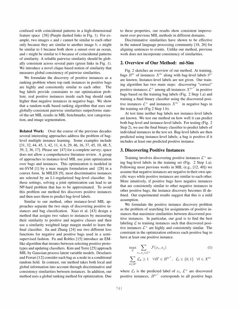
confused with coincidental patterns in a high-dimensionalfeature space [38] (Purple dashed links in Fig. 1). For ex-ample, two images a and c cannot be similar to each otheronly because they are similar to another image b; a mightbe similar to b because both show a sunset over an ocean,and c might be similar to b because of coincidental patternsof similarity. A reliable pairwise similarity should be glob-ally consistent across several pairs (green links in Fig. 1).We introduce a novel clique-based notion of similarity thatmeasures global consistency of pairwise similarities.

We formulate the discovery of positive instances as aranking problem where top rank instances in positive bagsare highly and consistently similar to each other. Thebag labels provide constraints to our optimization prob-lem; real positive instances inside each bag should rankhigher than negative instances in negative bags. We showthat a random-walk based ranking algorithm that uses ourglobally-consistent pairwise similarities outperforms state-of-the-art MIL results in MIL benchmarks, text categoriza-tion, and image segmentation.

Related Work: Over the course of the previous decadesseveral interesting approaches address the problem of bag-level multiple instance learning. Some examples include[31, 32, 44, 45, 1, 42, 11, 4, 6, 29, 46, 16, 37, 45, 10, 48, 5,39, 2, 36, 17]. Please see [47] for a complete survey; spacedoes not allow a comprehensive literature review. A groupof approaches to instance-level MIL use joint optimizationover bags and instances. This optimization is modeled inmi-SVM [1] by a max margin formulation and [28] in aconvex form. In MILES [9], most discriminative instancesare selected by an L1-regularized bag-level classifier. Inthese settings, solving a joint optimization can lead to anNP-hard problem that has to be approximated. To avoidthis problem our method firs discovers positive instancesand then uses them to predict bag-level labels.

Similar to our method, other instance-level MIL ap-proaches separate the two steps of discovering positive in-stances and bag classification. Xiao et al. [43] design amethod that assigns two values to instances by measuringtheir similarity to positive and negative classes and thenuse a similarity weighted large margin model to learn thefinal classifier. Jia and Zhang [24] use two different lossfunctions for negative and positive bags used in a semi-supervised fashion. Fu and Robles [15] introduce an EM-like algorithm that iterates between selecting positive proto-types and updating classifiers. Kim and Torre [25] approachMIL by Gaussian process latent variable models. Deselaersand Ferrari [12] consider each bag as a node in a conditionalrandom field. In contrast, our method takes both local andglobal information into account through discriminative andconsistency similarities between instances. In addition, ourmethod uses a global ranking method for optimization. Due

to these properties, our results show consistent improve-ment over previous MIL methods in different domains.

Discriminative similarities have shown to be effectivein the natural language processing community [18, 26] foraligning sentences to events. Unlike our method, previouswork does not incorporate consistency of similarities.

2. Overview of Our Method: mi-SimFig. 2 sketches an overview of our method. At training,

bags Btr of instances Xtr along with bag-level labels btr

are known; Instance-level labels are not given. Our train-ing algorithm has two main steps: discovering “correct”positive instances L+ among all instances Xtr+ in positivebags based on the training bag labels (Fig. 2 Step 1.a) andtraining a final binary classifier using the discovered posi-tive instances L+ and instances Xtr− in negative bags inthe training set (Fig 2 Step 1.b).

At test time neither bag labels nor instance-level labelsare known. We test our method on how well it can predictboth bag-level and instance-level labels. For testing (Fig. 2Step 2), we use the final binary classifier to predict labels ofindividual instances in the test set. Bag-level labels are thenpredicted using instance-level labels; a bag is positive if itincludes at least one predicted positive instance.

3. Discovering Positive InstancesTraining involves discovering positive instances L+ us-

ing bag-level labels in the training set (Fig. 2 Step 1.a).Following most previous works in MIL (e.g., [12, 40]) weassume that negative instances are negative in their own spe-cific ways while positive instances are similar to each other.More intuitively, if positive bags have negative instancesthat are consistently similar to other negative instances inother positive bags, the instance discovery becomes ill de-fined. Our experimental results suggest that this is a mildassumption.

We formulate the positive instance discovery problemas the problem of searching for assignments of positive in-stances that maximize similarities between discovered pos-itive instances. In particular, our goal is to find the bestlabeling L to training instances such that discovered posi-tive instances L+ are highly and consistently similar. Theconstraint in the optimization enforces each positive bag tohave at least one positive instance.

maxL

∑xi,xj∈L+

F(xi, xj) (1)

∑k∈B′

Lk ≥ 1 ∀B′ ∈ Btr+ , Ll ∈ {0, 1} ∀l ∈ Xtr

where Ll is the predicted label of xl, L+ are discoveredpositive instances, Btr+ corresponds to all positive bags

mi-Sim: Multiple Instance Learning• Let Btr be the set of training bags where every bag Btr

i has a binary label bi ∈ {−1, 1}• Let Xtr+ and Xtr− be the set of individual instances in positive and negative training bags, respectively• Let Btest be the set of bags at test time and Xtest be the set of all individual instances in test bags.• Let L+ be the set of discovered positive instances at training.

1. Training Phase(a) L+ ← Discovering positive instances from training examples (Sec.3)

i. Compute pairwise discriminative similarity S(xi, xj) (Sec. 3.1)A. Train iSVM with xi as the positive example and Xtr− as negative examples.B. S(xi, xj)← discriminative similarities between all instances in positive bags using Equation 3

ii. Compute consistency similarity C(xi, xj) (Sec. 3.2)iii. Select positive instances with ranking (Sec. 3.3)

A. CSG← the graph in which instances xi and xj are connected with a weight S(xi, xj) + C(xi, xj)B. Rxi

← the rank of each node xi in CSG with a random walk algorithm (Equation 6)C. L+ ← Pick top ranking instances based onRxi

in each bag as discovered positive instances(b) SVMfinal ← Train an SVM with L+ as positive examples and Xtr− as negative examples.

2. Testing Phase(a) Instance labes: L+

test ← set of test instances classified as positive using SVMfinal

(b) Bag labels: for every bag Btesti , assign a positive label if it includes at least one positive instance from L+

test

Figure 2. Our MIL method, mi-Sim, and discovering positive instances at training.

in the training set, and F is a form of similarity functionbetween pairs of instances xi and xj . Below we describehow to model F(xi, xj) as a combination of discriminativeS(xi, xj) and consistent similarities C(xi, xj).

Discriminative similarity: Positive instances should notonly be similar to each other but also be different from neg-ative instances. Learning a similarity function for positiveinstances require having a labeled set of positive instances,but instance-level labels are not available. We anchor thelearning of our similarity function on the only certain labelsin MIL setup; negative bag labels. All instances in the neg-ative bags are known to be negative. We propose to encodethe similarity between two positive instances based on howsimilarly they differ from negative instances (Sec. 3.1).

Consistency of similarities: Pairwise similarities are notalways transitive, they can be confused with coincidentalpatterns in the feature space [38]. For example, two im-ages may become similar because they both depict the samescene or may be similar because of some irrelevant acci-dents in the feature space. Coincidental patterns in the fea-ture space, by definition, are not repetitive. This suggeststhat a reliable pairwise similarity is the one that is homo-geneous across several pairs. We introduce the notion ofconsistent similarity and measure the consistency of a simi-larity based on the cardinality of the clique containing bothinstances (Sec. 3.2).

Positive instance discovery as ranking: We aim to dis-cover assignments of positive instances such that it maxi-mizes the similarities between positive instances, the dis-

crimination between positive and negative instances, andthe consistency of similarities between positive instances.Searching for the optimal assignments of instance labels isa challenging optimization problem that is even hard to ap-proximate. We formulate this problem by optimizing for aglobal ranking Rxu for each instance xu such that the toprank instances in each bag jointly maximize the similarityS and consistency C among positive instances:

maxR

∑xi,xj∈L+

S(xi, xj) + C(xi, xj) (2)

Rxu� Rxv

∀xu ∈ L+, xv ∈ (Xtr+ \ L+)

L+ = ∪n∆RBtrn

where Xtr+ corresponds to all the instances in positivebags, L+ is the discovered set of positive instances, Rxu

isthe ranking score of the instance xu in its bag, ∆RBtr

ncorre-

sponds to top-ranked instances based on rankingR in posi-tive bag Btr

n .Finding the optimal ordering of instances according to

the above optimization (Equation 2) is a challenging combi-natorial optimization problem (NP-Hard). We approximatethe above optimization with a random-walk based rank-ing that respects both similarity and consistency of simi-larities (Sec.3.3). To this end, we build a Consistent Sim-ilarity Graph (CSG) for instances in positive bags in thetraining set. Nodes in this graph are instances in posi-tive bags and edges represent discriminative pairwise sim-ilarities along with their consistency scores. The weight

of an edge between two nodes xi and xj correspond toS(xi, xj) + C(xi, xj).

Definition 1 (Consistent Similarity Graph (CSG)). A CSGis an undirected weighted graph CSG = (V,E) where anode xi ∈ V corresponds to a training instance xi in apositive bag and an edge eij ∈ E connects xi to xj , ifS(xi, xj) > 0. The weight eij is α.S(xi, xj) + C(xi, xj)where α is the balancing factor that takes into account thedifferences between the scales of S and C.

We approximate the best ranking by performing a ran-dom walk on this graph. The main intuition is nodes thatare adjacent to high rank nodes with large edge scores willget high ranks. There are several results on why a randomwalk based approach results in decent approximations of theoptimal ranking [33, 40, 34, 3, 35, 18, 26].

3.1. Pairwise Discriminative Similarity

In this section we describe how to derive similarityS(xi, xj) between two instances xi and xj (Fig.2 step 1.a.i).We base our notion of similarity on using negative labelswhich are the only certain labels in MIL. We learn whatis unique about each instance in positive bags by discrim-inating it from all instances in the negative bags; these arethe examples we are sure they are not similar to positive in-stances. We learn an instance by what it is not like. We dothis by fitting an SVM with only one positive instance anda large number of negative instances.

Recently in computer vision, Exemplar Support VectorMachines have shown great success in learning what isunique about an image that can distinguish it from all otherimages [30]. Despite being susceptible to overfitting, thehard negative mining method in [30] gets away from thisissue. By fitting a classifier to only one positive instanceand a large number of negative instances we learn how toweight features against each other in a discriminative man-ner. If a learned model for each instance produces a positivescore when applied to another instance, the two instancesare considered to be similar.

Based on our discriminative notion of similarity, two in-stances in positive bags are similar if they are similarly dif-ferent from negative instances. To setup notations, for aninstance xi ∈ Xtr+ , we fit a linear SVM (called iSVM) toxi as a positive training example and use instances Xtr− innegative bags as negative examples. We balance the posi-tive and negative examples by weighting them accordingly.The confidence of applying the SVM over a new instancexj is computed as Υi,j = wT

i · xj , where wi is the learnedweight vector for instance xi.

The discriminative similarity between two instances xiand xj is defined according to their mutual confidences.The confidence scores are not directly comparable. To cali-brate, we use the order of each instance among all the other

instances. The similarity of two instances xi and xj is1/ϕ(i, j).ϕ(j, i) where ϕ(i, j) represents the order of xjamong all the instances with positive confidence when clas-sified by wi.

S(xi, xj) =

{ 1ϕ(i,j)·ϕ(j,i) if Υi,j > 0 and Υj,i > 0

0 otherwise(3)

ϕ(i, j) is the rank of xj among all the training instances xkwhere Υi,k > 0.

3.2. Consistency of Similarities

In this section we describe how to compute the consis-tency C(xi, xj) of the similarity between two instances xiand xj (Fig.2 step 1.a.ii). Pairwise similarities are not al-ways transitive, they can be confused with coincidental pat-terns in the feature space [38]. This exposes subtleties toreasoning based on pairwise similarities. For example, twoimages may become similar because they both depict thesame scene or may be similar because of some irrelevant ac-cidents in the feature space. These accident happen largelybecause feature spaces are not perfect representations of theworld, and similarities are typically modeled by some sortof a global distance in a high dimensional space. Similar-ities typically expose several modalities out of which veryfew are desirable.

Coincidental patterns in the feature space, by definition,are not repetitive. This suggests that a reliable pairwise sim-ilarity is the one that is homogeneous across several pairs ina large clique of instances. We define a consistency scorebetween two instances as the size of the largest maximalclique that contains both instances. If a pairwise similarityis consistent then several homogeneous similarities can befound, thus the maximal clique is large in size. If a pair-wise similarity is not consistent the corresponding maximalclique is small, resulting in a small consistency score. InCSG the nodes are all the samples from positive bags andedges are only between nodes that their discriminative sim-ilarity are greater than zero.

The notion of a clique is slightly rigid for pairwise sim-ilarities due to uncertainties in our discriminative similaritymeasure and inherent variations among positive instances.For these reasons we use the notion of quasi-cliques [8] thatrelaxes the constraint of completeness in cliques.

Definition 2 (Quasi Clique). A graph G = (V,E) is a γ-quasi clique if |E| ≥ bγ

(|V |2

)c, where 0 < γ ≤ 1.

A quasi-clique essentially represents a group of instancesthat are densely similar to each other. Under settings ofMIL, it is natural to assume that positive instances corre-spond to higher cardinality quasi-cliques with high degreesof inner-clique-similarity.

Definition 3 (Maximal Quasi-Clique). A maximal quasi-clique in an undirected graph is a quasi-clique that cannotbe extended by adding any more node.

For each subgraph Gi induced by a node xi there alwaysexists a maximal quasi-clique containing xi. Every nodemight appear in more than one maximal quasi-clique.

We adopt a greedy approach [8] to find maximal quasi-cliques in a graph constructed by connecting similar in-stances in positive bags. For every node xi in CSG =(V,E), our method iteratively collects a set of verticesQi toform a quasi-clique corresponding to the node xi. Initially,Qi is set to xi. At each iteration a candidate set of instancesPi is a set of nodes xj ∈ V \ Qi that are connected to alarge portion of current nodes in Qi.

Pi =

{∀xj /∈ Qi,

∑xk∈Qi

1[ekj > 0] ≥ γ|Qi|

}(4)

where 1[.] is a 0-1 indicator function of its boolean argu-ment. Then, a node x∗j ∈ Pi will be added to Qi wherex∗j = arg maxxj∈Pi

∑xk∈Qi

ekj .

We iterate until there is no new node that can be addedto Qi i.e., Pi = ∅.

Corollary 1. Qi generated by the above algorithm returnsa maximal γ-quasi-clique.

Finally, we model consistency similarity between two in-stances xi and xj as the size of the largest maximal quasi-clique that includes the edge between xi and xj .

Definition 4 (Consistency Score). Let eij be the edge con-necting xi and xj in the graph. Let Qh denote differentmaximal quasi-cliques that include nodes xi and xj . Con-sistency C(xi, xj) of the edge eij is the size of the largestmaximal quasi-clique that includes both xi and xj .

C(xi, xj) =

{maxh{|Qh|} ∀h xi, xj ∈ Qh

0 @h xi, xj ∈ Qh

(5)

3.3. Ranking Instances in CSG

In this section we describe how to rank instances to op-timize for Equation 2 (Fig.2 step 1.a.iii). The optimal rank-ing imposes high consistent similarities among top rankedinstances in positive bags. To rank, we perform a random-walk algorithm to propagate scores in the consistent simi-larity graph. Recall that in CSG, we assign a node for eachinstance in positive bags. The edge scores are combinationsof discriminative similarity score and the consistency score.

We rank nodes in CSG by computing ranking scores ofall the instances Xtr+ in positive bags. We then selecthighest-scoring nodes as positive instances. The ranker in

CSG should assign high ranks to nodes which are highlyand consistently similar to many high rank instances. Weadopt a random walk algorithm similar to Google PageR-ank [7] that encourages propagating scores among edgesthat have high similarity score.

Our algorithm computes a ranking score Rxicorre-

sponding to every node in the graph. The algorithm iter-atively computes the score of a node according to Equation6. At every iteration, Rxi is the expected sum (with prob-ability d) of scores of the adjacent nodes (computed at theprevious iteration) and the self confidence value:

Rxi= (1− d)Υi,i + d

∑xj∈N (xi)

Rxj· eij (6)

where eij is the normalized weight of an edge in CSG, Υi,i

(as defined in section 3.1) is the confidence of each instanceclassifier on its own instance, N (xi) is the set of adjacentnodes to xi in CSG, and d is a damping factor. Rxi

is ini-tialized by random values.

At iteration 1, only direct edges (length 1) are consid-ered; Rxi only adds up the scores of the nodes that aredirectly linked to xi. In next iterations, longer paths areconsidered; the effect of indirectly linked nodes to xi is in-cluded in the scores of adjacent nodes. We control the ex-pected length of the paths with a damping factor d.

Once the scores of each instance is known, the mostprobable positives in each bag would be the highest scor-ing ones. In our experiments, we select positive instancesif their ranking score is higher than 0.9. Knowing the posi-tive instances in each bag, bag-level and instance-level MILbecome straight forward.

4. Experimental SetupTasks: We compare our method with bag-level andinstance-level state-of-the-art methods in different datasets.Training sets in all the experiments only include bag-levellabels. During training our method discovers positive in-stances in each bag. Once positive instances are discoveredwe train SVMfinal using discovered positive instances aspositive examples and all the examples in the negative bagsas negative instances. At test time, in bag-level classifica-tion, bag-level labels are inferred from the instance-levelpredictions. A bag will be positive if it contains at least onepredicted positive instance. In addition, we evaluate our al-gorithm for positive instance discovery (instance-level pre-dictions).Datasets: Benchmark datasets: We evaluate our methodon benchmark datasets for MIL including Drug ActivityPrediction (Musk1, Musk2) and Localized Content-basedImage Retrieval (Elephant, Tiger and Fox). More detailson these datasets can be found in [1].COREL-2000: We evaluate our method on COREL-2000,which is a standard dataset for image categorization using

MIL and has been studied by previous work in MIL. It con-tains 1000 images in 20 categories of COREL. For everyimage, regions are extracted via segmentation, and eachsegment represented by a 9-dimensional feature vector. Tocast image categorization to an MIL problem, every imageis a bag of regions. The regions are considered as instances.An image is positive if at least one of its regions contain theobject of interest. More details on this dataset can be foundin [10, 9].IL-MSRC: In order to evaluate instance-level MIL on imagecategorization tasks we introduce the Instance-level MSRC(IL-MSRC) dataset. We use images of MSRC dataset (30images per category). We perform segmentation on eachimage using superpixel extraction of [14]. We then useground-truth segments provided by MSRC to label each su-perpixel. A superpixel is positive, if it has more than 50%overlap (pixel area) with ground-truth segment otherwise itis negative. Images are bags and superpixels are instancesin each bag.20 Newsgroup: These datasets include texts from 20 news-groups corpora. This dataset has been introduced in mi-Graph [48] to evaluate the role of MIL in text categoriza-tion. Each dataset has 100 bags: 50 positive and 50 neg-ative. For every category, every positive bag includes afew news which are randomly selected for that categoryand many unrelated news. The main characteristic of thisdataset is that instance-level labels are available and it haslow witness rate (3%) i.e., there is almost one positive in-stance in each positive bag.

Parameters: Our method is not sensitive to the choice ofparameters across different domains. All the parameters arefixed across all the experiments except thresholding on thefinal SVM classifier. We have to do this because the litera-ture does not provide precision-recall values.

We set the parameter γ for finding quasi-cliques to 0.9in all the experiments across both texts and images. Weset α in Definition 1 to exp(10, blog

C(xi,xj)S(xi,xj)

c) to take intoaccount the differences between the scales of the similar-ity scores and consistency scores. Our ranking algorithmproduces a ranking score for all instances between 0 and1. Instances with a score higher than 0.9 is considered aspositive instance. For training iSVMs, the trade off param-eter c is default and we compensate for imbalanced data byweighting negative instances according to the size of thenegative set. Damping factor is set to 0.8 in all the exper-iments as suggested by Google. The final threshold overSVM scores are determined by cross-validation followingthe experimental setting in [28, 48]. To have an accuratecomparison, in each experiments we followed the settingsproposed by previous works on each experiment. Resultsof other methods are reported from the published work withthe exception of experiments on IL-MSRC where we usethe publicly available codes.

Algorithm Musk1 Musk2 Elephant Fox Tiger

mi-Sim 91.2±1.5 92.4±2.1 89.7±0.8 68.1±2.3 88.1±1.5Instance-level approaches

mi-SVM 87.4 83.6 82.0 58.2 78.9GPMIL 89.47 87.25 83.8 65.75 87.37SMILE 91.3 91.6 85.8 67.7 86.5MI-CRF 88.0 84.3 85.0 67.5 83.0MIMN 86 90 89 64 87MILES 86.3±1.4 87.7±1.4 N/A N/A N/AIL-SMIL 84.2±4.8 83.8±4.2 82.0±2.7 57.1±4.5 80.3±3.3SVR-SVM 87.9±1.7 85.4±1.8 85.3±2.8 63.0±3.5 79±3.4

Bag-level approachesmiGraph 88.9±3.3 90.3±2.6 86.8±0.7 61.6±2.8 86.0±1.6MIGraph 90.0±3.8 90.0±2.7 85.1±2.8 61.2±1.7 81.9±1.5MI-Kernel 88.0±3.1 89.3±1.5 84.3±1.6 60.3±1.9 84.2±1.6MI-SVM 77.9 84.3 81.4 59.4 84.0MissSVM 87.6 80.0 N/A N/A N/AMIForest 85 82 84 64 82MILboost 82.3 85.7 80.7 55.2 80.7DD 88.0 84.0 N/A N/A N/AEM-DD 84.8 84.9 78.3 56.1 72.1PPMM 95.6 81.2 82.4 60.3 82.4APR 92.4 89.2 N/A N/A N/A

Table 1. Accuracy of our method, mi-Sim, in predicting bag la-bels by our approach compared to state-of-the-art bag-level andinstance-level MIL approaches on benchmark tasks.

5. Experimental ResultsTo show the generality of our method, we apply our sys-

tem to different MIL benchmarks, image, and text domainsand show improvement over general MIL methods.5.1. Bag-Level Predictions

System Performance on Standard Benchmarks: Wecompare our method, mi-Sim, with previous bag-level andinstance-level methods for MIL on benchmark datasets. Wereport the accuracy of prediction of bag labels in percentvia ten times 10-fold cross validation. Our method out-performs all the other methods on all these datasets exceptPPMM[41] and APR[13] on Musk1. PPMM uses an ex-haustive search that may be prohibitive in practice. APRhas been designed specially for the drug activity prediction.System Performance on Text Categorization: MIL hasshown to be very effective in text categorization. Table 2(a)shows the results of comparisons on text categorization overtwenty datasets introduced in miGraph [48]. We report tentimes 10-fold cross validation following the experimentalsetting of miGraph and SVR-SVM [28]. Our method out-performs both methods in most datasets with a large mar-gin. The results can further be improved using more ad-vanced textual features to compute discriminative similari-ties [23, 19, 22, 20].System Performance on Image Categorization: Previ-

Table 2(a). Text Categorization

Dataset MI-Kernel miGraph miGraph-web SVR-SVM mi-Sim

alt.atheism 60.2 3.9 65.5±4.0 82.0±0.8 83.5±1.7 86.4±3.1comp.graphics 47.0±3.3 77.8±1.6 84.3±0.4 85.2±1.5 88.5±1.2comp.windows.misc 51.0±5.2 63.1±1.5 70.1±0.3 66.9±2.6 72.3±2.1comp.ibm.pc.hardware 46.9±3.6 59.5±2.7 79.4±0.8 70.3±2.8 85.3±3.2comp.sys.mac.hardware 44.5±3.2 61.7±4.8 81.0±0 78.0±1.7 85.1±1.8comp.window.x 50.8±4.3 69.8±2.1 79.4±0.5 83.7±2.0 86.3±1.7misc.forsale 51.8±2.5 55.2±2.7 71.0±0 72.3±1.2 77.6±2.7rec.autos 52.9±3.3 72.0±3.7 83.2±0.6 78.1±1.9 85.4±1.5rec.motorcycles 50.6±3.5 64.0±2.8 70.9±2.7 75.6±0.9 74.4±1.7rec.sport.baseball 51.7±2.8 64.7±3.1 75.0±0.6 76.7±1.4 82.4±2.3rec.sport.hockey 51.3±3.4 85.0±2.5 92.0±0 89.3±1.6 93.0±1.9sci.crypt 56.3±3.6 69.6±2.1 70.1±0.8 69.7±2.5 78.8±2.0sci.electronics 50.6±2.0 87.1±1.7 94.0±0 91.5±1.0 94.6±1.8sci.med 50.6±1.9 62.1±3.9 72.1±1.3 74.9±1.9 82.5±2.1sci.space 54.7±2.5 75.7±3.4 79.4±0.8 83.2±2.0 86.1±2.6soc.religion.christian 49.2±3.4 59.0±4.7 75.4±1.2 83.2±2.7 84.6±2.4talk.politics.guns 47.7±3.8 58.5±6.0 72.3±1.0 73.7±2.6 78.4±3.1talk.politics.mideast 55.9±2.8 73.6±2.6 75.5±1.0 80.5±3.2 85.3±2.1talk.politics.misc 51.5±3.7 70.4±3.6 72.9±2.4 72.6±1.4 76.1±2.6talk.religion.misc 55.4±4.3 63.3±3.5 67.5±1.0 71.9±1.9 80.6±4.9

Table 2(b). Image CategorizationDataset: COREL-2000

mi-Sim 74.2:[72.7,75.1]MIGraph 72.1:[71.0,73.2]miGraph 70.5:[68.7,72.3]MI-Kernel 72.0:[71.2,72.8]MI-SVM 54.6:[53.1,56.1]DD-SVM 67.5:[66.1,68.9]MissSVM 65.2:[62.0,68.3]MILES 68.7:[77.3,70.1]

Table 2(c). Dataset: IL-MSRC

mi-Sim 73.24BoW 64.2miGraph 70.12MI-SVM 67.32

Table 2(d). Ablation Study

Full System 88.1−Consistent 82.8−Discriminative 83.7−Ranking 82.1Gaussian 83.1

Table 2. Accuracy of our method, mi-Sim, vs. state of the art in predicting bag labels on (a) the text categorization task across differentdatasets (b) image categorization on the dataset COREL-2000, (c) image categorization on the dataset IL-MSRC, and (d) ablation study onthe benchmark Tiger dataset.

ous researchers show an interesting application of MIL inimage categorization. Tables 2(b) and (c) show the resultsof our method versus previous MIL techniques for imagecategorization on COREL2000 and IL-MSRC. We used thesame experimental setting as the previous work [48, 9] , re-peat five times 5-random partitioning, and report the overallaccuracy of 95% confidence intervals. For our new datasetIL-MSRC, we compared our method with BoW (simplebag-of-words model), MI-SVM, and mi-Graph (features areBOW of SIFT with 1000 codebooks). Our method out-performs all the previous techniques with a large margin.The results can further be improved using more advancedvision-based features to compute discriminative similari-ties [27].

Contribution of System Components: Table 2(d)shows the accuracy for different controls on benchmarkdatasets to show the importance of each of the com-ponents. (−consistency) removes consistent similaritiesand only considers pairwise discriminative similarities,(−discriminative) removes discriminative similarities andonly considers consistent similarities on edges. (−ranking)replaces random walk ranking with a baseline of using thedegree of each node as its final score; this baseline examinesthe importance of our random walk algorithm to approxi-mate optimization 2. (Gaussian) replaces the discriminativesimilarity with ε-graph of Gaussian similarity in a same way

as it is proposed in miGraph (highest competition with oursystem). Results shows that each component in our modelplays an important role in our final system and removingeach component drops the performance with a big margin.

System Running Time: Our system, for every instance,trains one iSVM which is a linear classifier and can belearned efficiently. We compare the running time of our fullsystem with miGraph and miSVM on Tiger dataset whichhas 1220 instances and 200 bags. The training time (in sec-ond) of our method, miGraph and miSVM are 3.23, 3.12,856 respectively and testing times are 2.51, 2.71, 2.63. Inaddition, the training time of our method for each iSVMclassifier in MSRC dataset takes less than 0.5 sec.

5.2. Instance-Level Predictions

Table 1 shows that our method outperforms previousinstance-level MIL methods in bag-level predictions. Toshow that our approach is also successful in instance-levelpredictions, we evaluate our system on 20 Newsgroups andour new dataset IL-MSRC that include instance-level labels.

20 Newsgroups: Figure 3 compares the instance-level ac-curacy for our method and mi-SVM[1] on all the datasetsin the 20 newsgroup using F1-measure. Positive instancesfound by our method and mi-SVM are those that have high-est score within each bag. We significantly outperform mi-SVM in all those datasets.

mi-­‐S

VM  

Ours  

Images  

Tree   House   Cow   Airplane   Face   Bicycle   Car  

Figure 4. Positive Instance Discovery: Our method is capable of discovering positive instances (superpixels that correspond to the objectof interest) in bags(images). (left) The first row shows 7 images from IL-MSRC. The second and third rows show discovered superpixelsusing miSVM and our method, respectively. (right) Precision-Recall curve for instance-level predictions in IL-MSRC

!"

!#$"

!#%"

!#&"

!#'"

!#("

!#)"

!#*"

!#+"

!#,"

-./0

123"

45-6/172"

819:;

82#3127

"67#/-5:8

-50"

3-7#/-5:8

-50"

819:;

82#<"

=;52->0"

-?.;2"

3;.;57@7>02"

A-20A->>"

/;7B0@"

271#75@6."

271#0>07.5;9172"

271#3

0:"

271#26-70"

7/512C-

9"6;

>1C72#4?9

2"6;

>1C72#3

1:0-2."

6;>1C

72#3

127"

50>141;9#3127

"

!"#

$%&'#

()*+,-#

Figure 3. Instance-level predictions in Newsgroup 20

Instance-level MSRC: The task is to find which super-pixel corresponds to the object of interest. Figure 4(right),shows the precision-recall curve on the IL-MSRC dataset.The precision-recall curve is traced by a threshold on theinstance-level scores. Positive instances are those that areabove a threshold (T ) within each bag. We do this becausethere could be several positive instances in each bag. Ourmethod significantly outperforms mi-SVM. Figure 4(left)depicts qualitative examples of the regions discovered byour method and mi-SVM. Note that image segmentation isnot the focus of this paper. We used this task to showcasethe generality of our approach. Our features are very simpleand we avoid any vision specific tweaks to be comparablewith other MIL methods.

6. Conclusion and Future Work

In this paper we show improvement over the state-of-the-art MIL methods by reasoning about discriminative andconsistent similarities. Our method is widely applicable;We show our method produces promising results across textand vision tasks with no change. One potential case of fail-

ure of our method is when positive examples are very dif-ferent from each other and hence they do not follow anyparticular structure. Under this setting, many other MILmethods would fail as well.

Pairwise similarities are modeled by discriminating eachinstance from known negative instances (the only certainlabels in MIL). This requires training one SVM for everyinstance. This is computationally less attractive. However,each exemplar SVM is a linear SVM and these classifierscan be learned efficiently in parallel. Since we have a fixedset of negative examples, the computation of exemplar clas-sifiers can be very fast using whitening techniques [21].Pairwise similarities are not always transitive. This meansthat reasoning based on pairwise similarities should be ob-servant about the kind of similarities being utilized. In thispaper we show that by measuring the consistency of simi-larities one can select “good” similarities to reason about.This leads to more reliable discovery of positive instances.

Discovering positive instances using only pairwise simi-larities is a typical example of discovering a global structureby aggregating local evidences. This is a challenging taskthat appears in a lot of machine learning problems and issusceptible to having issues with local optimum. By aug-menting the local evidence with global or structural cuesone can aim for better local optimum. This makes local rea-soning to be more informed about the global structure. Theconsistency of similarities, at least in the way we model it,can be thought of as a structural cue that is coupled withlocal cues, pairwise similarities.

References

[1] Andrews, Tsochantaridis, and Hofmann. SVMs for multiple-instance learning. In NIPS, 2003.

[2] S. Andrews and T. Hofmann. Multiple instance learning viadisjunctive programming boosting. In NIPS, 2004.

[3] Arasu, Cho, Garcia-Molia, Paepcke, and Raghavan. Search-ing the web. ACM Trans. on internet technologies, 2001.

[4] P. Auer. On learning from multi-instance examples. InICML, 1997.

[5] Babenko, Varma, Dollar, and Belongie. Multiple instancelearning with manifold bags. In ICML, 2011.

[6] A. Blum and A. Kalai. A note on learning from multiple-instance examples. Kluwer Academic Publishers, 1997.

[7] S. Brin and L. Page. The anatomy of a large-scale hypertex-tual web search engine. Computer Networks, 1998.

[8] Brunato, Hoos, and Battiti. On effectively finding maximalquasi-cliques in graphs. In CLIO, 2007.

[9] Chen, Bi, and Wang. Miles: Multiple-instance learning viaembedded instance selection. TPAMI, 2006.

[10] Chen and Wang. Image categorization by learning and rea-soning with regions. JMLR’04, 2007.

[11] Chevaleyre and Zucker. Solving multiple-instance andmultiple-part learning problems with decision trees and rulesets. In AAI, 2001.

[12] Deselaers and Ferrari. A conditional random field formultiple-instance learning. In ICML, 2010.

[13] Dietterich., Lathrop, and Lozano. Solving the multiple in-stance problem with axis-parallel rectangles. AI, 1997.

[14] Felzenszwalb and Huttenlocher. Efficient graph-based imagesegmentation. IJCV, 2004.

[15] Fu and Robles. An instance selection approach to multipleinstance learning. In CVPR, 2009.

[16] Gehler and Chapelle. Deterministic annealing for mil.JMLR’07, 2007.

[17] H. Hajimirsadeghi, J. Li, G. Mori, M. Zaki, and T. Sayed.Multiple instance learning by discriminative training ofmarkov networks. In UAI, pages 262–271, 2013.

[18] H. Hajishirzi, M. Rastegari, A. Farhadi, and J. Hodgins. Se-mantic understanding of professional soccer commentaries.In UAI, 2012.

[19] H. Hajishirzi, W.-t. Yih, and A. Kolcz. Adaptive near-duplicate detection via similarity learning. In ACM SIGIR,pages 419–426, 2010.

[20] H. Hajishirzi, L. Zilles, D. S. Weld, and L. S. Zettlemoyer.Joint coreference resolution and named-entity linking withmulti-pass sieves. In EMNLP, 2013.

[21] B. Hariharan, J. Malik, and D. Ramanan. Discriminativedecorrelation for clustering and classification. In ECCV,2012.

[22] M. J. Hosseini, H. Hajishirzi, O. Etzioni, and N. Kushman.Learning to solve arithmetic word problems with verb cate-gorization. In EMNLP, 2014.

[23] W. Hwang, H. Hajishirzi, M. Ostendorf, and W. Wu. Align-ing sentences from standard wikipedia to simple wikipedia.In NAACL, 2015.

[24] Jai and Zhang. Instance-level semisupervised multiple in-stance learning. In AAAI08, 2008.

[25] M. Kim and F. D. la Torre. Gaussian processes multiple in-stance learning. In ICML, 2010.

[26] R. Koncel-Kedziorski, H. Hajishirzi, and A. Farhadi. Multi-resolution language grounding with weak supervision. InEMNLP, pages 386–396, 2014.

[27] A. Krizhevsky, I. Sutskever, and G. E. Hinton. Imagenetclassification with deep convolutional neural networks. InNIPS, pages 1097–1105. 2012.

[28] Li and Sminchisescu. Convex multiple-instance learning byestimating likelihood ratio. In NIPS, 2010.

[29] Long and Tan. Pac learning axis-aligned rectangles with re-spect to product distributions from multiple-instance exam-ples. In COLT, 1996.

[30] T. Malisiewicz, A. Gupta, and A. Efros. Ensemble ofexemplar-svms for object detection. In ICCV, 2011.

[31] O. Maron and T. Lozano-Prez. A framework for multiple-instance learning. In NIPS, 1996.

[32] O. Maron and A. L. Ratan. Multiple-instance learning fornatural scene classification. In ICML, 1998.

[33] R. Mihalcea and D. Radev. Graph-based Natural LanguageProcessing and Information Retrieval. Cambridge Univer-sity Press, 2011.

[34] Muthukrishnan, Radev, and Mei. Simultaneous similaritylearning and feature-weight learning for document cluster-ing. In TextGraphs, 2011.

[35] Picardello and Woess. Random walks and discrete potentialtheory. 2000.

[36] W. Ping, Y. Xu, J. Wang, and X.-S. Hua. FAMER: Makingmulti-instance learning better and faster. In SDM, 2011.

[37] Scott, Zhang, and Brown. On generalized multiple-instancelearning. In IJCAI, 2003.

[38] A. Shrivastava, T. Malisiewicz, A. Gupta, and A. A. Efros.Data-driven visual similarity for cross-domain image match-ing. Proceedings of ACM SIGGRAPH ASIA, 2011.

[39] Viola, Platt, and Zhang. Multiple instance boosting for objectdetection. In NIPS, 2006.

[40] Wang, Li, and Zhang. Multiple-instance learning via randomwalk. In ECML, 2006.

[41] Wang, Yang, and Zha. Adaptive p-posterior mixture-modelkernels for mil. ICML, 2008.

[42] J. Wang, Zucker, and Jean-Daniel. Solving multiple-instanceproblem: A lazy learning approach. In ICML, 2000.

[43] Xiao, Liu, Cao, Jie, and Wu. Smile: A similarity-based ap-proach for multiple instance learning. In ICDM, 2010.

[44] C. Yang. Image database retrieval with multiple-instancelearning techniques. In ICDE, 2000.

[45] Zhang, Goldman, Yu, and Fritts. Content-based image re-trieval using mil. In ICML, 2002.

[46] Q. Zhang and S. A. Goldman. EM-DD: An improvedmultiple-instance learning technique. In NIPS, 2001.

[47] Zhou. Multi-instance learning: A survey. In TR. AI LabDepartment of Computer Science Technology Nanjing Uni-versity, 2004.

[48] Zhou, Sun, and Li. Multi-instance learning by treating in-stances as non-i.i.d. samples. In ICML, 2009.