Discrete uncertainty principles and sparse signal processing

Afonso S. Bandeira∗ Megan E. Lewis† Dustin G. Mixon‡

May 26, 2017

Abstract

We develop new discrete uncertainty principles in terms of numerical sparsity, which is acontinuous proxy for the 0-norm. Unlike traditional sparsity, the continuity of numerical sparsitynaturally accommodates functions which are nearly sparse. After studying these principles andthe functions that achieve exact or near equality in them, we identify certain consequences in anumber of sparse signal processing applications.

1 Introduction

Uncertainty principles have maintained a significant role in both science and engineering for mostof the past century. In 1927, the concept was introduced by Werner Heisenberg in the context ofquantum mechanics [24], in which a particle’s position and momentum are represented by wave-functions f, g ∈ L2(R), and g happens to be the Fourier transform of f . Measuring the position ormomentum of a particle amounts to drawing a random variable whose probability density functionis a normalized version of |f |2 or |g|2, respectively. Heisenberg’s uncertainty principle postulates afundamental limit on the precision with which one can measure both position and momentum; inparticular, the variance of the position measurement is small only if the momentum measurementexhibits large variance. From a mathematical perspective, this physical principle can be viewed asan instance of a much broader meta-theorem in harmonic analysis:

A nonzero function and its Fourier transform cannot be simultaneously localized.

Heisenberg’s uncertainty principle provides a lower bound on the product of the variances ofthe probability density functions corresponding to f and f . In the time since, various methodshave emerged for quantifying localization. For example, instead of variance, one might considerentropy [6], the size of the density’s support [2], or how rapidly it decays [23]. Furthermore, thetradeoff in localization need not be represented by a product—as we will see, it is sometimes moretelling to consider a sum.

Beyond physics, the impossibility of simultaneous localization has had significant consequencesin signal processing. For example, when working with the short-time Fourier transform, one isforced to choose between temporal and frequency resolution. More recently, the emergence ofdigital signal processing has prompted the investigation of uncertainty principles underlying thediscrete Fourier transform, notably by Donoho and Stark [17], Tao [42], and Tropp [44]. Associatedwith this line of work is the uniform uncertainty principle of Candes and Tao [12], which played akey role in the development of compressed sensing. The present paper continues this investigationof discrete uncertainty principles with an eye on applications in sparse signal processing.

∗Department of Mathematics, Courant Institute of Mathematical Sciences, New York University, New York, NY†Detachment 5, Air Force Operational Test and Evaluation Center, Edwards AFB, CA‡Department of Mathematics and Statistics, Air Force Institute of Technology, Wright-Patterson AFB, OH

1

arX

iv:1

504.

0101

4v3

[cs

.IT

] 2

5 M

ay 2

017

1.1 Background and overview

For any finite abelian group G, let `(G) denote the set of functions x : G → C, and G ⊆ `(G) thegroup of characters over G. Then taking inner products with these characters and normalizingleads to the (unitary) Fourier transform F : `(G)→ `(G), namely

(Fx)[χ] :=1√|G|

∑g∈G

x[g]χ[g] ∀χ ∈ G.

The reader who is unfamiliar with Fourier analysis over finite abelian groups is invited to learn morein [43]. In the case where G = Z/nZ (which we denote by Zn in the sequel), the above definitioncoincides with the familiar discrete Fourier transform after one identifies characters with theirfrequencies. The following theorem provides two uncertainty principles in terms of the so-called0-norm ‖ · ‖0, defined to be number of nonzero entries in the argument.

Theorem 1 (Theorem 1 in [17], Theorem 1.1 in [42]). Let G be a finite abelian group, and letF : `(G)→ `(G) denote the corresponding Fourier transform. Then

‖x‖0‖Fx‖0 ≥ |G| ∀x ∈ `(G) \ 0. (1)

Furthermore, if |G| is prime, then

‖x‖0 + ‖Fx‖0 ≥ |G|+ 1 ∀x ∈ `(G) \ 0. (2)

Proof sketch. For (1), apply the fact that the `1/`∞-induced norm of F is given by ‖F‖1→∞ =1/√|G|, along with Cauchy–Schwarz and Parseval’s identity:

‖Fx‖∞ ≤1√|G|‖x‖1 ≤

√‖x‖0|G|‖x‖2 =

√‖x‖0|G|‖Fx‖2 ≤

√‖x‖0‖Fx‖0|G|

‖Fx‖∞,

where the last step bounds a sum in terms of its largest summand. Rearranging gives the result.For (2), suppose otherwise that there exists x 6= 0 which violates the claimed inequality. Denote

J = supp(x) and pick some I ⊆ G \ supp(Fx) with |I| = |J |. Then 0 = (Fx)I = FIJ xJ . Sincethe submatrix FIJ is necessarily invertible by a theorem of Chebotarev [39], we conclude thatxJ = 0, a contradiction.

We note that the additive uncertainty principle above is much stronger than its multiplica-tive counterpart. Indeed, with the help of the arithmetic mean–geometric mean inequality, (1)immediately implies

‖x‖0 + ‖Fx‖0 ≥ 2√‖x‖0‖Fx‖0 ≥ 2

√|G| ∀x ∈ `(G), (3)

which is sharp when G = Zn and n is a perfect square (simply take x to be a Dirac comb, specifically,the indicator function 1K of the subgroup K of size

√n). More generally, if n is not prime, then

n = ab with integers a, b ∈ [2, n/2], and so a + b ≤ n/2 + 2 < n + 1; as such, taking x to be anindicator function of the subgroup of size a (whose Fourier transform necessarily has 0-norm b) willviolate (2). Overall, the hypothesis that |G| is prime cannot be weakened. Still, something can besaid if one slightly strengthens the hypothesis on x. For example, Theorem A in [46] gives that forevery S ⊆ G,

‖x‖0 + ‖Fx‖0 >√|G|‖x‖0

2

−100 −80 −60 −40 −20 0 20 40 60 80 100

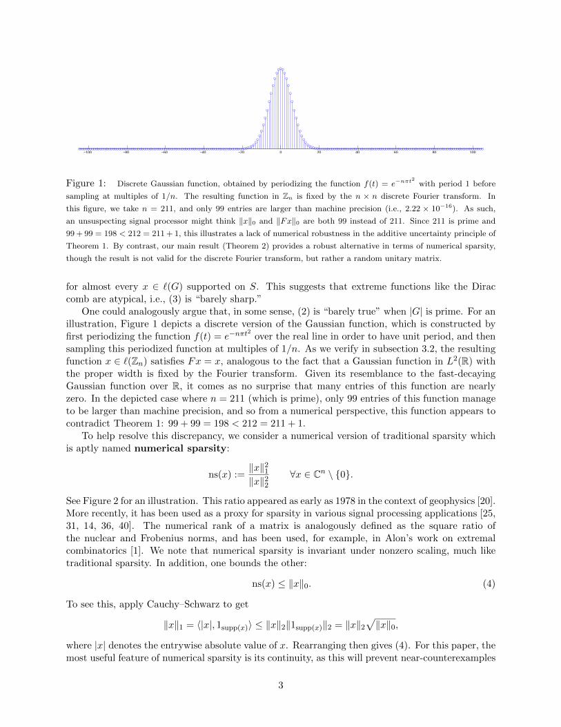
Figure 1: Discrete Gaussian function, obtained by periodizing the function f(t) = e−nπt2

with period 1 before

sampling at multiples of 1/n. The resulting function in Zn is fixed by the n × n discrete Fourier transform. In

this figure, we take n = 211, and only 99 entries are larger than machine precision (i.e., 2.22 × 10−16). As such,

an unsuspecting signal processor might think ‖x‖0 and ‖Fx‖0 are both 99 instead of 211. Since 211 is prime and

99 + 99 = 198 < 212 = 211 + 1, this illustrates a lack of numerical robustness in the additive uncertainty principle of

Theorem 1. By contrast, our main result (Theorem 2) provides a robust alternative in terms of numerical sparsity,

though the result is not valid for the discrete Fourier transform, but rather a random unitary matrix.

for almost every x ∈ `(G) supported on S. This suggests that extreme functions like the Diraccomb are atypical, i.e., (3) is “barely sharp.”

One could analogously argue that, in some sense, (2) is “barely true” when |G| is prime. For anillustration, Figure 1 depicts a discrete version of the Gaussian function, which is constructed byfirst periodizing the function f(t) = e−nπt

2over the real line in order to have unit period, and then

sampling this periodized function at multiples of 1/n. As we verify in subsection 3.2, the resultingfunction x ∈ `(Zn) satisfies Fx = x, analogous to the fact that a Gaussian function in L2(R) withthe proper width is fixed by the Fourier transform. Given its resemblance to the fast-decayingGaussian function over R, it comes as no surprise that many entries of this function are nearlyzero. In the depicted case where n = 211 (which is prime), only 99 entries of this function manageto be larger than machine precision, and so from a numerical perspective, this function appears tocontradict Theorem 1: 99 + 99 = 198 < 212 = 211 + 1.

To help resolve this discrepancy, we consider a numerical version of traditional sparsity whichis aptly named numerical sparsity:

ns(x) :=‖x‖21‖x‖22

∀x ∈ Cn \ 0.

See Figure 2 for an illustration. This ratio appeared as early as 1978 in the context of geophysics [20].More recently, it has been used as a proxy for sparsity in various signal processing applications [25,31, 14, 36, 40]. The numerical rank of a matrix is analogously defined as the square ratio ofthe nuclear and Frobenius norms, and has been used, for example, in Alon’s work on extremalcombinatorics [1]. We note that numerical sparsity is invariant under nonzero scaling, much liketraditional sparsity. In addition, one bounds the other:

ns(x) ≤ ‖x‖0. (4)

To see this, apply Cauchy–Schwarz to get

‖x‖1 = 〈|x|, 1supp(x)〉 ≤ ‖x‖2‖1supp(x)‖2 = ‖x‖2√‖x‖0,

where |x| denotes the entrywise absolute value of x. Rearranging then gives (4). For this paper, themost useful feature of numerical sparsity is its continuity, as this will prevent near-counterexamples

3

Figure 2: Traditional sparsity ‖x‖0 (left) and numerical sparsity ns(x) (right) for all x in the unit circle in R2. This

illustrates how numerical sparsity is a continuous analog of traditional sparsity; we leverage this feature to provide

robust alternatives to the uncertainty principles of Theorem 1. In this case, one may verify that ns(x) ≤ ‖x‖0 by

visual inspection.

like the one depicted in Figure 1. What follows is our main result, which leverages numericalsparsity to provide uncertainty principles that are analogous to those in Theorem 1:

Theorem 2 (Main result1). Let U be an n× n unitary matrix. Then

ns(x) ns(Ux) ≥ 1

‖U‖21→∞∀x ∈ Cn \ 0, (5)

where ‖ · ‖1→∞ denotes the induced matrix norm. Furthermore, there exists a universal constantc > 0 such that if U is drawn uniformly from the unitary group U(n), then with probability 1−e−Ω(n),

ns(x) + ns(Ux) ≥ (c− o(1))n ∀x ∈ Cn \ 0. (6)

Perhaps the most glaring difference between Theorems 1 and 2 is our replacement of the Fouriertransform with an arbitrary unitary matrix. Such generalizations have appeared in the quantumphysics literature (for example, see [29]), as well as in the sparse signal processing literature [16,15, 21, 44, 46, 40]. Our multiplicative uncertainty principle still applies when U = F , in whichcase ‖U‖1→∞ = 1/

√n. Considering (4), the uncertainty principle in this case immediately implies

the analogous principle in Theorem 1. Furthermore, the proof is rather straightforward: ApplyHolder’s inequality to get

ns(x) ns(Ux) =‖x‖21‖x‖22

· ‖Ux‖21

‖Ux‖22≥ ‖x‖

21

‖x‖22· ‖Ux‖

22

‖Ux‖2∞=‖x‖21‖Ux‖2∞

≥ 1

‖U‖21→∞. (7)

By contrast, the proof of our additive uncertainty principle is not straightforward, and it doesnot hold if we replace U with F . Indeed, as we show in subsection 3.2, the discrete Gaussianfunction depicted in Figure 1 has numerical sparsity O(

√n), thereby violating (6); recall that the

same function is a near-counterexample of the analogous principle in Theorem 1. Interestingly,

1Recall that f(n) = O(g(n)) if there exists C, n0 > 0 such that f(n) ≤ Cg(n) for all n > n0. We writef(n) = Oδ(g(n)) if the constant C is a function of δ. Also, f(n) = Ω(g(n)) if g(n) = O(f(n)), and f(n) = o(g(n)) iff(n)/g(n)→ 0 as n→∞.

4

our uncertainty principle establishes that the Fourier transform is rare in that the vast majorityof unitary matrices offer much more uncertainty in the worst case. This naturally leads to thefollowing question:

Problem 3. For each n, what is the largest c = c(n) for which there exists a unitary matrix Uthat satisfies ns(x) + ns(Ux) ≥ cn for every x ∈ Cn \ 0?

Letting x = e1 gives ns(x) + ns(Ux) ≤ 1 + ‖Ux‖0 ≤ n + 1, and so c(n) ≤ 1 + o(1); a bit morework produces a strict inequality c(n) < 1 + 1/n for n ≥ 4. Also, our proof of the uncertaintyprinciple implies lim infn→∞ c(n) ≥ 1/540000.

1.2 Outline

The primary focus of this paper is Theorem 2. Having already proved the multiplicative uncertaintyprinciple in (7), it remains to prove the additive counterpart, which we do in the following section.Next, Section 3 considers functions which achieve either exact or near equality in (5) when U isthe discrete Fourier transform. Surprisingly, exact equality occurs in (5) precisely when it occursin (1). We also show that the discrete Gaussian depicted in Figure 1 achieves near equality in(5). We conclude in Section 4 by studying a few applications, specifically, sparse signal demixing,compressed sensing with partial Fourier operators, and the fast detection of sparse signals.

2 Proof of additive uncertainty principle

In this section, we prove the additive uncertainty principle in Theorem 2. The following providesa more explicit statement of the principle we prove:

Theorem 4. Draw U uniformly from the unitary group U(n). Then with probability ≥ 1−8e−n/4096,

ns(x) + ns(Ux) ≥ 1

9

⌊ n

60000

⌋∀x ∈ Cn \ 0.

For the record, we did not attempt to optimize the constants. Our proof of this theorem makesuse of several ideas from the compressed sensing literature:

Definition 5. Take any m× n matrix Φ = [ϕ1 · · ·ϕn].

(a) We say Φ exhibits (k, θ)-restricted orthogonality if

|〈Φx,Φy〉| ≤ θ‖x‖2‖y‖2

for every x, y ∈ Cn with ‖x‖0, ‖y‖0 ≤ k and disjoint support.

(b) We say Φ satisfies the (k, δ)-restricted isometry property if

(1− δ)‖x‖22 ≤ ‖Φx‖22 ≤ (1 + δ)‖x‖22

for every x ∈ Cn with ‖x‖0 ≤ k.

(c) We say Φ satisfies the (k, c)-width property if

‖x‖2 ≤c√k‖x‖1

for every x in the nullspace of Φ.

5

The restricted isometry property is a now-standard sufficient condition for uniformly stableand robust reconstruction from compressed sensing measurements (for example, see [11]). As thefollowing statement reveals, restricted orthogonality implies the restricted isometry property:

Lemma 6 (Lemma 11 in [4]). If a matrix satisfies (k, θ)-restricted orthogonality and its columnshave unit norm, then it also satisfies the (k, δ)-restricted isometry property with δ = 2θ.

To prove Theorem 4, we will actually make use of the width property, which was introducedby Kashin and Temlyakov [27] to characterize uniformly stable `1 reconstruction for compressedsensing. Luckily, the restricted isometry property implies the width property:

Lemma 7 (Theorem 11 in [9], cf. [27]). If a matrix satisfies the (k, δ)-restricted isometry propertyfor some positive integer k and δ < 1/3, then it also satisfies the (k, 3)-width property.

What follows is a stepping-stone result that we will use to prove Theorem 4, but it is also ofindependent interest:

Theorem 8. Draw U uniformly from the unitary group U(n). Then [I U ] satisfies the (k, δ)-restricted isometry property with probability ≥ 1− 8e−δ

2n/256 provided δ < 1 and

n ≥ 256

δ2k log

(en

k

). (8)

This is perhaps not surprising, considering various choices of structured random matrices areknown to form restricted isometries with high probability [12, 37, 35, 28, 34, 8, 3]. To prove The-orem 8, we show that the structured matrix enjoys restricted orthogonality with high probability,and then appeal to Lemma 6. Before proving this result, we first motivate it by proving the desireduncertainty principle:

Proof of Theorem 4. Take k = bn/60000c and δ = 1/4. We will show ns(x) + ns(Ux) ≥ k/9 forevery nonzero x ∈ Cn. If k = 0, the result is immediate, and so n ≥ 60000 without loss of generality.In this regime, we have k ∈ [n/120000, n/60000], and so

256

δ2k log

(en

k

)≤ 4096 log(120000e) · k ≤ 60000k ≤ n.

Theorem 8 and Lemma 7 then give that [I U ] satisfies the (k, 3)-width property with probability≥ 1− 8e−n/4096. Observe that z = [Ux;−x] resides in the nullspace of [I U ] regardless of x ∈ Cn.In the case where x (and therefore z) is nonzero, the width property and the arithmetic mean–geometric mean inequality together give

k

9≤ ‖z‖

21

‖z‖22=

(‖x‖1 + ‖Ux‖1)2

‖x‖22 + ‖Ux‖22=‖x‖21 + 2‖x‖1‖Ux‖1 + ‖Ux‖21

2‖x‖22≤ ns(x) + ns(Ux).

Proof of Theorem 8. Take [I U ] = [ϕ1 · · ·ϕ2n], and let k be the largest integer satisfying (8). Wewill demonstrate that [I U ] satisfies the (k, δ)-restricted isometry property, which will then implythe (k′, δ)-restricted isometry property for all k′ < k+ 1, and therefore all k satisfying (8). To thisend, define the random quantities

θ?(U) := maxx,y∈C2n

‖x‖0,‖y‖0≤ksupp(x)∩supp(y)=∅

|〈Φx,Φy〉|‖x‖2‖y‖2

, θ(U) := maxx,y∈C2n

‖x‖0,‖y‖0≤ksupp(x)⊆[n]supp(y)⊆[n]c

|〈Φx,Φy〉|‖x‖2‖y‖2

.

6

We first claim that θ?(U) ≤ θ(U). To see this, for any x, y satisfying the constraints in θ?(U),decompose x = x1 + x2 so that x1 and x2 are supported in [n] and [n]c, respectively, and similarlyy = y1 + y2. For notational convenience, let S denote the set of all 4-tuples (a, b, c, d) of k-sparsevectors in C2n such that a and b are disjointly supported in [n], while c and d are disjointly supportedin [n]c. Then (x1, y1, x2, y2) ∈ S. Since supp(x) and supp(y) are disjoint, and since I and U eachhave orthogonal columns, we have

〈Φx,Φy〉 = 〈Φx1,Φy2〉+ 〈Φx2,Φy1〉.

As such, the triangle inequality gives

θ?(U) = maxx,y∈C2n

‖x‖0,‖y‖0≤ksupp(x)∩supp(y)=∅

|〈Φx1,Φy2〉+ 〈Φx2,Φy1〉|‖x‖2‖y‖2

≤ max(x1,y1,x2,y2)∈S

|〈Φx1,Φy2〉|+ |〈Φx2,Φy1〉|√‖x1‖22 + ‖x2‖22

√‖y1‖22 + ‖y2‖22

≤(

max(x1,y1,x2,y2)∈S

‖x1‖2‖y2‖2 + ‖x2‖2‖y1‖2√‖x1‖22 + ‖x2‖22

√‖y1‖22 + ‖y2‖22

)θ(U)

≤ θ(U),

where the last step follows from squaring and applying the arithmetic mean–geometric mean in-equality: ( √

ad+√bc√

(a+ b)(c+ d)

)2

=ad+ bc+ 2

√acbd

(a+ b)(c+ d)≤ ad+ bc+ (ac+ bd)

(a+ b)(c+ d)= 1.

At this point, we seek to bound the probability that θ(U) is large. First, we observe an equivalentexpression:

θ(U) = maxx,y∈Cn

‖x‖2=‖y‖2=1‖x‖0,‖y‖0≤k

|〈x, Uy〉|.

To estimate the desired probability, we will pass to an ε-net Nε of k-sparse vectors with unit 2-norm.A standard volume-comparison argument gives that the unit sphere in Rm enjoys an ε-net of size≤ (1 + 2/ε)m (see Lemma 5.2 in [47]). As such, for each choice of k coordinates, we can cover thecorresponding copy of the unit sphere in Ck = R2k with ≤ (1 + 2/ε)2k points, and unioning theseproduces an ε-net of size

|Nε| ≤(n

k

)(1 +

2

ε

)2k

.

To apply this ε-net, we note that ‖x− x′‖2, ‖y − y′‖2 ≤ ε and ‖x′‖2 = ‖y′‖2 = 1 together imply

|〈x, Uy〉| = |〈x′ + x− x′, U(y′ + y − y′)〉|≤ |〈x′, Uy′〉|+ ‖x− x′‖2 + ‖y − y′‖2 + ‖x− x′‖2‖y − y′‖2≤ |〈x′, Uy′〉|+ 3ε,

7

where the last step assumes ε ≤ 1. As such, the union bound gives

Pr(θ(U) > t) = Pr

(∃x, y ∈ Cn, ‖x‖2 = ‖y‖2 = 1, ‖x‖0, ‖y‖0 ≤ k s.t. |〈x, Uy〉| > t

)≤ Pr

(∃x, y ∈ Nε s.t. |〈x, Uy〉| > t− 3ε

)≤

∑x,y∈Nε

Pr(|〈x, Uy〉| > t− 3ε

)=

(n

k

)2(1 +

2

ε

)4k

Pr(|〈e1, Ue1〉| > t− 3ε

), (9)

where the last step uses the fact that the distribution of U is invariant under left- and right-multiplication by any deterministic unitary matrix (e.g., unitary matrices that send e1 to x and yto e1, respectively). It remains to prove tail bounds on U11 := 〈e1, Ue1〉. First, we apply the unionbound to get

Pr(|U11| > u) ≤ Pr

(|Re(U11)| > u√

2

)+ Pr

(| Im(U11)| > u√

2

)= 4 Pr

(Re(U11) >

u√2

), (10)

where the last step uses the fact that Re(U11) has even distribution. Next, we observe that Re(U11)has the same distribution as g/

√h, where g has standard normal distribution and h has chi-squared

distribution with 2n degrees of freedom. Indeed, this can be seen from one method of constructingthe matrix U : Start with an n× n matrix G with iid N(0, 1) + iN(0, 1) complex Gaussian entriesand apply Gram–Schmidt to the columns; the first column of U is then the first column of G dividedby its norm

√h. Let s > 0 be arbitrary (to be selected later). Then g/

√h > u/

√2 implies that

either g >√su/√

2 or h < s. As such, the union bound implies

Pr

(Re(U11) >

u√2

)≤ 2 max

Pr

(g >√su√2

),Pr(h < s)

. (11)

For the first term, Proposition 7.5 in [19] gives

Pr

(g >√su√2

)≤ e−su2/4. (12)

For the second term, Lemma 1 in [30] gives Pr(h < 2n −√

8nx) ≤ e−x for any x > 0. Pickingx = (2n− s)2/(8n) then gives

Pr(h < s) ≤ e−(2n−s)2/(8n). (13)

We use the estimate(nk

)≤ (en/k)k when combining (9)–(13) to get

log(

Pr(θ(U) > t))≤ 2k log

(en

k

)+ 4k log

(1 +

2

ε

)+ log 8−min

s(t− 3ε)2

4,(2n− s)2

8n

.

Notice n/k ≥ (256/δ2) log(en/k) ≥ 256 implies that taking ε =√

(k/n) log(en/k) gives√en

k− 2

ε=

(1− 2√

e log(n/k)

)√en

k≥(

1− 2√e log(256)

)√256e ≥ 1,

which can be rearranged to get

log

(1 +

2

ε

)≤ 1

2log

(en

k

).

8

As such, we also pick s = n and t =√

(64k/n) log(en/k) to get

log(

Pr(θ(U) > t))≤ 4k log

(en

k

)+ log 8− 25

4k log

(en

k

)≤ log 8− 2k log

(en

k

).

Since we chose k to be the largest integer satisfying (8), we therefore have θ(U) ≤√

(64k/n) log(n/k)

with probability ≥ 1− 8e−δ2n/256. Lemma 6 then gives the result.

3 Low uncertainty with the discrete Fourier transform

In this section, we study functions which achieve either exact or near equality in our multiplicativeuncertainty principle (6) in the case where the unitary matrix U is the discrete Fourier transform.

3.1 Exact equality in the multiplicative uncertainty principle

We seek to understand when equality is achieved in (6) in the special case of the discrete Fouriertransform. For reference, the analogous result for (1) is already known:

Theorem 9 (Theorem 13 in [17]). Suppose x ∈ `(Zn) satisfies ‖x‖0‖Fx‖0 = n. Then x has theform x = cT aM b1K , where c ∈ C, K is a subgroup of Zn, and T,M : `(Zn)→ `(Zn) are translationand modulation operators defined by

(Tx)[j] := x[j − 1], (Mx)[j] := e2πij/nx[j] ∀j ∈ Zn.

Here, i denotes the imaginary unit√−1.

In words, equality is achieved in (1) by indicator functions of subgroups, namely, the so-calledDirac combs (as well as their scalar multiples, translations, modulations). We seek an analogouscharacterization for our uncertainty principle (6). Surprisingly, the characterization is identical:

Theorem 10. Suppose x ∈ `(Zn). Then ns(x) ns(Fx) = n if and only if ‖x‖0‖Fx‖0 = n.

Proof. (⇐) This follows directly from (4), along with Theorems 1 and 2.(⇒) It suffices to show that ns(x) = ‖x‖0 and ns(Fx) = ‖Fx‖0. Note that both F and F−1 are

unitary operators and ‖F‖21→∞ = ‖F−1‖21→∞ = 1/n. By assumption, taking y := Fx then gives

ns(F−1y) ns(y) = ns(x) ns(Fx) = n.

We will use the fact that x and y each achieve equality in the first part of Theorem 2 with U = Fand U = F−1, respectively. Notice from the proof (7) that equality occurs only if x and y satisfyequality in Holder’s inequality, that is,

‖x‖1‖x‖∞ = ‖x‖22, ‖y‖1‖y‖∞ = ‖y‖22. (14)

To achieve the first equality in (14),∑j∈Zn

|x[j]|2 = ‖x‖22 = ‖x‖1‖x‖∞ =∑j∈Zn

|x[j]|maxk∈Zn

|x[k]|.

This implies that |x[j]| = maxk |x[k]| for every j with x[j] 6= 0. Similarly, in order for the secondequality in (14) to hold, |y[j]| = maxk |y[k]| for every j with y[j] 6= 0. As such, |x| = a1A and|y| = b1B for some a, b > 0 and A,B ⊆ Zn. Then

ns(x) =‖x‖21‖x‖22

=(a|A|)2

a2|A|= |A| = ‖x‖0,

and similarly, ns(y) = ‖y‖0.

9

3.2 Near equality in the multiplicative uncertainty principle

Having established that equality in the new multiplicative uncertainty principle (5) is equivalentto equality in the analogous principle (1), we wish to separate these principles by focusing on nearequality. For example, in the case where n is prime, Zn has no nontrivial proper subgroups, andso by Theorem 9, equality is only possible with identity basis elements and complex exponentials.On the other hand, we expect the new principle to accommodate nearly sparse vectors, and so weappeal to the discrete Gaussian depicted in Figure 1:

Theorem 11. Define x ∈ `(Zn) by

x[j] :=∑j′∈Z

e−nπ( jn

+j′)2 ∀j ∈ Zn. (15)

Then Fx = x and ns(x) ns(Fx) ≤ (2 + o(1))n.

In words, the discrete Gaussian achieves near equality in the uncertainty principle (5). Moreover,numerical evidence suggests that ns(x) ns(Fx) = (2 + o(1))n, i.e., the 2 is optimal for the discreteGaussian. Note that this does not depend on whether n is prime or a perfect square. Recall that afunction f ∈ C∞(R) is Schwarz if supx∈R |xαf (β)(x)| < ∞ for every pair of nonnegative integersα and β. We use this to quickly prove a well-known lemma that will help us prove Theorem 11:

Lemma 12. Suppose f ∈ C∞(R) is Schwarz and construct a discrete function x ∈ `(Zn) byperiodizing and sampling f as follows:

x[j] =∑j′∈Z

f

(j

n+ j′

)∀j ∈ Zn. (16)

Then the discrete Fourier transform of x is determined by f(ξ) :=∫∞−∞ f(t)e−2πiξtdt:

(Fx)[k] =√n∑k′∈Z

f(k + k′n) ∀k ∈ Zn.

Proof. Since f is Schwarz, we may apply the Poisson summation formula:

x[j] =∑j′∈Z

f

(j

n+ j′

)=∑l∈Z

f(l)e2πijl/n.

Next, the geometric sum formula gives

(Fx)[k] =1√n

∑j∈Zn

(∑l∈Z

f(l)e2πijl/n

)e−2πijk/n

=1√n

∑l∈Z

f(l)∑j∈Zn

(e2πi(l−k)/n

)j=√n

∑l∈Z

l≡k mod n

f(l).

The result then follows from a change of variables.

Proof of Theorem 11. It is straightforward to verify that the function f(t) = e−nπt2

is Schwarz.Note that defining x according to (16) then produces (15). Considering f(ξ) = n−1/2e−πξ

2/n, onemay use Lemma 12 to quickly verify that Fx = x. To prove Theorem 11, it then suffices to showthat ns(x) ≤ (

√2 + o(1))

√n. We accomplish this by bounding ‖x‖2 and ‖x‖1 separately.

10

To bound ‖x‖2, we first expand a square to get

‖x‖22 =∑j∈Zn

(∑j′∈Z

e−nπ( jn

+j′)2)2

=∑j∈Zn

∑j′∈Z

∑j′′∈Z

e−nπ[( jn

+j′)2+( jn

+j′′)2].

Since all of the terms in the sum are nonnegative, we may infer a lower bound by discarding theterms for which j′′ 6= j′. This yields the following:

‖x‖22 ≥∑j∈Zn

∑j′∈Z

e−2nπ( jn

+j′)2 =∑k∈Z

e−2πk2/n ≥∫ ∞−∞

e−2πx2/ndx− 1 =

√n

2− 1,

where the last inequality follows from an integral comparison. Next, we bound ‖x‖1 using a similarintegral comparison:

‖x‖1 =∑j∈Zn

∑j′∈Z

e−nπ( jn

+j′)2 =∑k∈Z

e−πk2/n ≤

∫ ∞−∞

e−πx2/ndx+ 1 =

√n+ 1.

Overall, we have

ns(x) =‖x‖21‖x‖22

≤ (√n+ 1)2√n/2− 1

= (√

2 + o(1))√n.

4 Applications

Having studied the new uncertainty principles in Theorem 2, we now take some time to identifycertain consequences in various sparse signal processing applications. In particular, we reportconsequences in sparse signal demixing, in compressed sensing with partial Fourier operators, andin the fast detection of sparse signals.

4.1 Sparse signal demixing

Suppose a signal x is sparse in the Fourier domain and corrupted by noise ε which is sparse in thetime domain (such as speckle). The goal of demixing is to recover the original signal x given thecorrupted signal z = x + ε; see [32] for a survey of various related demixing problems. ProvidedFx and ε are sufficiently sparse, it is known that this recovery can be accomplished by solving

v? := argmin ‖v‖1 subject to [I F ]v = Fz, (17)

where, if successful, the solution v? is the column vector obtained by concatenating Fx and ε; see [38]for an early appearance of this sort of approach. To some extent, we know how sparse Fx and ε mustbe for this `1 recovery method to succeed. Coherence-based guarantees in [16, 15, 21] show that itsuffices for v? to be k-sparse with k = O(

√n), while restricted isometry–based guarantees [11, 5]

allow for k = O(n) if [I F ] is replaced with a random matrix. This disparity is known as thesquare-root bottleneck [45]. In particular, does [I F ] perform similarly to a random matrix, oris the coherence-based sufficient condition on k also necessary?

In the case where n is a perfect square, it is well known that the coherence-based sufficientcondition is also necessary. Indeed, let K denote the subgroup of Zn of size

√n and suppose

x = 1K and ε = −1K . Then [Fx; ε] is 2√n-sparse, and yet z = 0, thereby forcing v? = 0. On the

other hand, if n is prime, then the additive uncertainty principle of Theorem 1 implies that everymember of the nullspace of [I F ] has at least n + 1 nonzero entries, and so v? 6= 0 in this setting.

11

Still, considering Figure 1, one might expect a problem from a stability perspective. In this section,we use numerical sparsity to show that Φ = [I F ] cannot break the square-root bottleneck, even ifn is prime. To do this, we will make use of the following theorem:

Theorem 13 (see [27, 9]). Denote ∆(y) := argmin ‖x‖1 subject to Φx = y. Then

‖∆(Φx)− x‖2 ≤C√k‖x− xk‖1 ∀x ∈ Rn (18)

if and only if Φ satisfies the (k, c)-width property. Furthermore, C c in both directions of theequivalence.

Take x as defined in (15). Then [x;−x] lies in the nullspace of [I F ] and

ns([x;−x]) =(2‖x‖1)2

2‖x‖22= 2 ns(x) ≤ (2

√2 + o(1))

√n,

where the last step follows from the proof of Theorem 11. As such, [I F ] satisfies the (k, c)-widthproperty for some c independent of n only if k = O(

√n). Furthermore, Theorem 13 implies that

stable demixing by `1 reconstruction requires k = O(√n), thereby proving the necessity of the

square-root bottleneck in this case.It is worth mentioning that the restricted isometry property is a sufficient condition for (18)

(see [11], for example), and so by Theorem 8, one can break the square-root bottleneck by replacingthe F in [I F ] with a random unitary matrix. This gives a uniform demixing guarantee which issimilar to those provided by McCoy and Tropp [33], though the convex program they considerdiffers from (17).

4.2 Compressed sensing with partial Fourier operators

Consider the random m×n matrix obtained by drawing rows uniformly with replacement from then× n discrete Fourier transform matrix. If m = Ωδ(k polylog n), then the resulting partial Fourieroperator satisfies the restricted isometry property, and this fact has been dubbed the uniformuncertainty principle [12]. A fundamental problem in compressed sensing is determining thesmallest number m of random rows necessary. To summarize the progress to date, Candes andTao [12] first found that m = Ωδ(k log6 n) rows suffice, then Rudelson and Vershynin [37] provedm = Ωδ(k log4 n), and recently, Bourgain [8] achieved m = Ωδ(k log3 n); Nelson, Price and Woot-ters [34] also achieved m = Ωδ(k log3 n), but using a slightly different measurement matrix. Inthis subsection, we provide a lower bound: in particular, m = Ωδ(k log n) is necessary whenever kdivides n. Our proof combines ideas from the multiplicative uncertainty principle and the classicalproblem of coupon collecting.

The coupon collector’s problem asks how long it takes to collect all k coupons in an urn if yourepeatedly draw one coupon at a time randomly with replacement. It is a worthwhile exercise toprove that the expected number of trials scales like k log k. We will require even more informationabout the distribution of the random number of trials:

Theorem 14 (see [18, 13]). Let Tk denote the random number of trials it takes to collect k differentcoupons, where in each trial, a coupon is drawn uniformly from the k coupons with replacement.

(a) For each a ∈ R,

limk→∞

Pr(Tk ≤ k log k + ak

)= e−e

−(a+γ),

where γ ≈ 0.5772 denotes the Euler–Mascheroni constant.

12

(b) There exists c > 0 such that for each k,

supa∈R

∣∣∣∣Pr(Tk ≤ k log k + ak

)− e−e−(a+γ)

∣∣∣∣ ≤ c log k

k.

Lemma 15. Suppose k divides n, and draw m iid rows uniformly from the n× n discrete Fouriertransform matrix to form a random m×n matrix Φ. If m < k log k, then the nullspace of Φ containsa k-sparse vector with probability ≥ 0.4− c(log k)/k, where c is the constant from Theorem 14(b).

Proof. Let K denote the subgroup of Zn of size k, and let 1K denote its indicator function. Weclaim that some modulation of 1K resides in the nullspace of Φ with the probability reported inthe lemma statement. Let H denote the subgroup of Zn of size n/k. Then the Fourier transform ofeach modulation of 1K is supported on some coset of H. Letting M denote the random row indicesthat are drawn uniformly from Zn, a modulation of 1K resides in the nullspace of Φ precisely whenM fails to intersect the corresponding coset of H. As there are k cosets, each with probability 1/k,this amounts to a coupon-collecting problem (explicitly, each “coupon” is a coset, and we “collect”the cosets that M intersects). The result then follows immediately from Theorem 14(b):

Pr(Tk ≤ m) ≤ e−e−(m/k−log k+γ)+c log k

k≤ e−e−γ +

c log k

k≤ 0.6 +

c log k

k.

Presumably, one may remove the divisibility hypothesis in Lemma 15 at the price of weakeningthe conclusion. We suspect that the new conclusion would declare the existence of a vector x ofnumerical sparsity k such that ‖Φx‖2 ‖x‖2. If so, then Φ fails to satisfy the so-called robustwidth property, which is necessary and sufficient for stable and robust reconstruction by `1minimization [9]. For the sake of simplicity, we decided not to approach this, but we suspect thatmodulations of the discrete Gaussian would adequately fill the role of the current proof’s modulatedindicator functions.

What follows is the main result of this subsection:

Theorem 16. Let k be sufficiently large, suppose k divides n, and draw m iid rows uniformly fromthe n × n discrete Fourier transform matrix to form a random m × n matrix Φ. Take δ < 1/3.Then Φ satisfies the (k, δ)-restricted isometry property with probability ≥ 2/3 only if

m ≥ C(δ)k log(en),

where C(δ) is some constant depending only on δ.

Proof. In the event that Φ satisfies (k, δ)-RIP, we know that no k-sparse vector lies in the nullspaceof Φ. Therefore, Lemma 15 implies

m ≥ k log k, (19)

since otherwise Φ fails to be (k, δ)-RIP with probability ≥ 0.4−c(log k)/k > 1/3, where the last stepuses the fact that k is sufficiently large. Next, we leverage standard techniques from compressedsensing: (k, δ)-RIP implies (18) with C = C1(δ) (see Theorem 3.3 in [10]), which in turn implies

m ≥ C2(δ)k log

(en

k

)(20)

by Theorem 11.7 in [19]. Since Φ is (k, δ)-RIP with positive probability, we know there exists anm× n matrix which is (k, δ)-RIP, and so m must satisfy (20). Combining with (19) then gives

m ≥ max

k log k,C2(δ)k log

(en

k

).

13

The result then follows from applying the bound maxa, b ≥ (a + b)/2 and then taking C(δ) :=(1/2) min1, C2(δ).

We note that the necessity of k log n random measurements contrasts with the proportional-growth asymptotic adopted in [7] to study the restricted isometry property of Gaussian matrices.Indeed, it is common in compressed sensing to consider phase transitions in which k, m and n aretaken to infinity with fixed ratios k/m and m/n. However, since random partial Fourier operatorsfail to be restricted isometries unless m = Ωδ(k log n), such a proportional-growth asymptotic failsto capture the so-called strong phase transition of these operators [7].

The proof of Theorem 16 relies on the fact that the measurements are drawn at random. Bycontrast, it is known that every m× n partial Hadamard operator fails to satisfy (k, δ)-RIP unlessm = Ωδ(k log n) [41, 22]. We leave the corresponding deterministic result in the Fourier case forfuture work.

4.3 Fast detection of sparse signals

The previous subsection established fundamental limits on the number of Fourier measurementsnecessary to perform compressed sensing with a uniform guarantee. However, for some applications,signal reconstruction is unnecessary. In this subsection, we consider one such application, namelysparse signal detection, in which the goal is to test the following hypotheses:

H0 : x = 0

H1 : ‖x‖22 =n

k, ‖x‖0 ≤ k.

Here, we assume we know the 2-norm of the sparse vector we intend to detect, and we set it to be√n/k without loss of generality (this choice of scaling will help us interpret our results later). We

will assume the data is accessed according to the following query–response model:

Definition 17 (Query–response model). If the ith query is ji ∈ Zn, then the ith response is(Fx)[ji] + εi, where the εi’s are iid complex random variables with some distribution such that

E|εi| = α, E|εi|2 = β2.

The coefficient of variation v of |εi| is defined as

v =

√Var |εi|E|εi|

=

√β2 − α2

α. (21)

Note that for any scalar c 6= 0, the mean and variance of |cεi| are |c|α and |c|2 Var |εi|, respectively.As such, v is scale invariant and is simply a quantification of the “shape” of the distribution of |εi|.We will evaluate the responses to our queries with an `1 detector, defined below.

Definition 18 (`1 detector). Fix a threshold τ . Given responses yimi=1 from the query–responsemodel, if

m∑i=1

|yi| > τ,

then reject H0.

The following is the main result of this section:

14

Theorem 19. Suppose α ≤ 1/(8k). Randomly draw m indices uniformly from Zn with replacement,input them into the query–response model and apply the `1 detector with threshold τ = 2mα to theresponses. Then

Pr

(reject H0

∣∣∣∣ H0

)≤ p (22)

and

Pr

(fail to reject H0

∣∣∣∣ H1

)≤ p (23)

provided m ≥ (8k + 2v2)/p, where v is the coefficient of variation defined in (21).

In words, the probability that the `1 detector delivers a false positive is at most p, as is theprobability that it delivers a false negative. These error probabilities can be estimated better givenmore information about the distribution of the random noise, and presumably, the threshold τ canbe modified to decrease one error probability at the price of increasing the other. Notice that weonly use O(k) samples in the Fourier domain to detect a k-sparse signal. Since the sampled indicesare random, it will take O(log n) bits to communicate each query, leading to a total computa-tional burden of O(k log n) operations. This contrasts with the state-of-the-art sparse fast Fouriertransform algorithms which require Ω(k log(n/k)) samples and take O(k polylog n) time (see [26]and references therein). We suspect k-sparse signals cannot be detected with substantially fewersamples (in the Fourier domain or any domain).

We also note that the acceptable noise magnitude α = O(1/k) is optimal in some sense. Tosee this, consider the case where k divides n and x is a properly scaled indicator function of thesubgroup of size k. Then Fx is the indicator function of the subgroup of size n/k. (Thanks toour choice of scaling, each nonzero entry in the Fourier domain has unit magnitude.) Since aproportion of 1/k entries is nonzero in the Fourier domain, we can expect to require O(k) randomsamples in order to observe a nonzero entry, and the `1 detector will not distinguish the entry fromaccumulated noise unless α = O(1/k).

Before proving Theorem 19, we first prove a couple of lemmas. We start by estimating theprobability of a false positive:

Lemma 20. Take ε1, . . . , εm to be iid complex random variables with E|εi| = α and E|εi|2 = β2.Then

Pr

( m∑i=1

|εi| > 2mα

)≤ p

provided m ≥ v2/p, where v is the coefficient of variation of |εi| defined in (21).

Proof. Denoting X :=∑m

i=1 |εi|, we have EX = mα and VarX = m(β2 − α2). Chebyshev’sinequality then gives

Pr

( m∑i=1

|εi| −mα > t

)≤ Pr(|X − EX| > t) ≤ VarX

t2=m(β2 − α2)

t2.

Finally, we take t = mα to get

Pr

( m∑i=1

|εi| > 2mα

)≤ m(β2 − α2)

(mα)2=β2 − α2

mα2≤ β2 − α2

α2· pv2

= p.

Next, we leverage the multiplicative uncertainty principle in Theorem 2 to estimate momentsof noiseless responses:

15

Lemma 21. Suppose ‖x‖0 ≤ k and ‖x‖22 = n/k. Draw j uniformly from Zn and define Y :=|(Fx)[j]|. Then

EY ≥ 1

k, EY 2 =

1

k.

Proof. Recall that ns(x) ≤ ‖x‖0 ≤ k. With this, Theorem 2 gives

n ≤ ns(x) ns(Fx) ≤ k ns(Fx).

We rearrange and apply the definition of numerical sparsity to get

n

k≤ ns(Fx) =

‖Fx‖21‖Fx‖22

=‖Fx‖21‖x‖22

=‖Fx‖21n/k

,

where the second to last equality is due to Parseval’s identity. Thus, ‖Fx‖1 ≥ n/k. Finally,

EY =1

n

∑j∈Zn

|(Fx)[j]| = 1

n‖Fx‖1 ≥

1

k

and

EY 2 =1

n

∑j∈Zn

|(Fx)[j]|2 =1

n‖Fx‖22 =

1

k.

Proof of Theorem 19. Lemma 20 gives (22), and so it remains to prove (23). Denoting Yi :=|(Fx)[ji]|, we know that |yi| ≥ Yi − |εi|, and so

Pr

( m∑i=1

|yi| ≤ 2ma

)≤ Pr

( m∑i=1

Yi −m∑i=1

|εi| ≤ 2ma

). (24)

For notational convenience, put Z :=∑m

i=1 Yi −∑m

i=1 |εi|. We condition on the size of the noiseand apply Lemma 20 with the fact that m ≥ v2/(p/2) to bound (24):

Pr(Z ≤ 2mα) = Pr

(Z ≤ 2mα

∣∣∣∣ m∑i=1

|εi| > 2mα

)Pr

( m∑i=1

|εi| > 2mα

)

+ Pr

(Z ≤ 2mα

∣∣∣∣ m∑i=1

|εi| ≤ 2mα

)Pr

( m∑i=1

|εi| ≤ 2mα

)

≤ p

2+ Pr

( m∑i=1

Yi ≤ 4mα

). (25)

Now we seek to bound the second term of (25). Taking X =∑m

i=1 Yi, Lemma 21 gives EX ≥ m/kand VarX = mVarYi ≤ mEY 2

i = m/k. As such, applying Chebyshev’s inequality gives

Pr

( m∑i=1

Yi <m

k− t)≤ Pr(X ≤ EX − t) ≤ Pr(|X − EX| > t) ≤ Var(X)

t2≤ m

kt2.

Recalling that α ≤ 1/(8k), we take t = m/(2k) to get

Pr

( m∑i=1

Yi ≤ 4mα

)≤ Pr

( m∑i=1

Yi ≤m

2k

)= Pr

( m∑i=1

Yi ≤m

k− t)≤ m

kt2=

4k

m≤ p

2, (26)

where the last step uses the fact that m ≥ 8k/p. Combining (24), (25), and (26) gives the result.

16

Acknowledgments

The authors thank Laurent Duval, Joel Tropp, and the anonymous referees for multiple suggestionsthat significantly improved the presentation of our results and our discussion of the relevant liter-ature. ASB was supported by AFOSR Grant No. FA9550-12-1-0317. DGM was supported by anAFOSR Young Investigator Research Program award, NSF Grant No. DMS-1321779, and AFOSRGrant No. F4FGA05076J002. The views expressed in this article are those of the authors and donot reflect the official policy or position of the United States Air Force, Department of Defense, orthe U.S. Government.

References

[1] N. Alon, Problems and results in extremal combinatorics, Discrete Math. 273 (2003) 31–53.

[2] W. O. Amrein, A. M. Berthier, On support properties of Lp-functions and their Fouriertransforms, J. Funct. Anal. 24 (1977) 258–267.

[3] A. S. Bandeira, M. Fickus, D. G. Mixon, J. Moreira, Derandomizing restricted isometriesvia the Legendre symbol, Available online: arXiv:1406.4089

[4] A. S. Bandeira, M. Fickus, D. G. Mixon, P. Wong, The road to deterministic matrices withthe restricted isometry property, J. Fourier Anal. Appl. 19 (2013) 1123–1149.

[5] R. Baraniuk, M. Davenport, R. DeVore, M. Wakin, A simple proof of the restricted isometryproperty for random matrices, Constr. Approx. 28 (2008) 253–263.

[6] W. Beckner, Inequalities in Fourier analysis, Ann. Math. 102 (1975) 159–182.

[7] J. D. Blanchard, C. Cartis, J. Tanner, Compressed sensing: How sharp is the restrictedisometry property?, SIAM Rev. 53 (2011) 105–125.

[8] J. Bourgain, An improved estimate in the restricted isometry problem, Lect. Notes Math.2116 (2014) 65–70.

[9] J. Cahill, D. G. Mixon, Robust width: A characterization of uniformly stable and robustcompressed sensing, Available online: arXiv:1408.4409

[10] T. T. Cai, A. Zhang, Sharp RIP bound for sparse signal and low-rank matrix recovery, Appl.Comput. Harmon. Anal. 35 (2013) 74–93.

[11] E. J. Candes, The restricted isometry property and its implications for compressed sensing,C. R. Acad. Sci. Paris, Ser. I 346 (2008) 589–592.

[12] E. J. Candes, T. Tao, Near-optimal signal recovery from random projections: Universalencoding strategies?, IEEE Trans. Inform. Theory 52 (2006) 5406–5425

[13] S. Csorgo, A rate of convergence for coupon collectors, Acta Sci. Math. (Szeged) 57 (1993)337–351.

[14] L. Demanet, P. Hand, Scaling law for recovering the sparsest element in a subspace, Availableonline: arXiv:1310.1654

17

[15] D. L. Donoho, M. Elad, Optimally sparse representation in general (nonorthogonal) dictio-naries via `1 minimization, Proc. Natl. Acad. Sci. U.S.A. 100 (2003) 2197–2202.

[16] D. L. Donoho, X. Huo, Uncertainty principles and ideal atomic decomposition, IEEE Trans.Inform. Theory 47 (2001) 2845–2862.

[17] D. L. Donoho, P. B. Stark, Uncertainty principles and signal recovery, SIAM J. Appl. Math.49 (1989) 906–931.

[18] P. Erdos, A. Renyi, On a classical problem of probability theory, Magyar Tud. Akad. Mat.Kutato Int. Kozl. 6 (1961) 215–220.

[19] A. Foucart, H. Rauhut, A Mathematical Introduction to Compressive Sensing, Applied andNumerical Harmonic Analysis, Birkhauser, 2013.

[20] W. C. Gray, Variable norm deconvolution, Tech. Rep. SEP-14, Stanford University, 1978.

[21] R. Gribonval, M. Nielsen, Highly sparse representations from dictionaries are unique andindependent of the sparseness measure, Appl. Comput. Harmon. Anal. 22 (2007) 335–355.

[22] O. Guedon, S. Mendelson, A. Pajor, N. Tomczak-Jaegermann, Majorizing measures andproportional subsets of bounded orthonormal systems, Rev. Mat. Iberoam. 24 (2008) 1075–1095.

[23] G. H. Hardy, A theorem concerning Fourier transforms, J. London Math. Soc. 8 (1933)227–231.

[24] W. Heisenberg, Uber den anschaulichen Inhalt der quantentheoretischen Kinematik undMechanik, Z. Phys. (in German) 43 (1927) 172–198.

[25] N. Hurley, S. Rickard, Comparing measures of sparsity, IEEE Trans. Inform. Theory 55(2009) 4723–4741.

[26] P. Indyk, M. Kapralov, Sample-optimal Fourier sampling in any constant dimension, FOCS2014, 514–523.

[27] B. S. Kashin, V. N. Temlyakov, A remark on compressed sensing, Math. Notes 82 (2007)748–755.

[28] F. Krahmer, S. Mendelson, H. Rauhut, Suprema of chaos processes and the restricted isom-etry property, Comm. Pure Appl. Math. 67 (2014) 1877–1904.

[29] K. Kraus, Complementary observables and uncertainty relations, Phys. Rev. D 35 (1987)3070–3075.

[30] B. Laurent, P. Massart, Adaptive estimation of a quadratic functional by model selection,Ann. Statist. 28 (2000) 1302–1338.

[31] M. E. Lopes, Estimating unknown sparsity in compressed sensing, JMLR W&CP 28 (2013)217–225.

[32] M. B. McCoy, V. Cevher, Q. T. Dinh, A. Asaei, L. Baldassarre, Convexity in source sepa-ration: Models, geometry, and algorithms, Signal Proc. Mag. 31 (2014) 87–95.

18

[33] M. B. McCoy, J. A. Tropp, Sharp recovery bounds for convex demixing, with applications,Found. Comput. Math. 14 (2014) 503–567.

[34] J. Nelson, E. Price, M. Wootters, New constructions of RIP matrices with fast multiplicationand fewer rows, SODA 2014, 1515–1528.

[35] H. Rauhut, Compressive sensing and structured random matrices, Theoretical foundationsand numerical methods for sparse recovery 9 (2010) 1–92.

[36] A. Repetti, M. Q. Pham, L. Duval, E. Chouzenoux, J.-C. Pesquet, Euclid in a taxicab:Sparse blind deconvolution with smoothed `1/`2 regularization, IEEE Signal Process. Lett.22 (2014) 539–543.

[37] M. Rudelson, R. Vershynin, On sparse reconstruction from Fourier and Gaussian measure-ments, Comm. Pure Appl. Math. 61 (2008) 1025–1045.

[38] F. Santosa, W. W. Symes, Linear inversion of band-limited reflection seismograms, SIAMJ. Sci. Statist. Comp. 7 (1986) 1307–1330.

[39] P. Stevenhagen, H. W. Lenstra, Chebotarev and his density theorem, Math. Intelligencer18 (1996) 26–37.

[40] C. Studer, Recovery of signals with low density, Available online: arXiv:1507.02821

[41] M. Talagrand, Selecting a proportion of characters, Israel J. Math. 108 (1998) 173–191.

[42] T. Tao, An uncertainty principle for cyclic groups of prime order, Math. Research Lett. 12(2005) 121–127.

[43] A. Terras, Fourier Analysis on Finite Groups and Applications, Cambridge University Press,1999.

[44] J. A. Tropp, On the linear independence of spikes and sines, J. Fourier Anal. Appl. 14 (2008)838–858.

[45] J. A. Tropp, On the conditioning of random subdictionaries, Appl. Comput. Harmon. Anal.25 (2008) 1–24.

[46] J. A. Tropp, The sparsity gap: Uncertainty principles proportional to dimension, CISS 2010,1–6.

[47] R. Vershynin, Introduction to the non-asymptotic analysis of random matrices, CompressedSensing: Theory and Applications, Cambridge University Press, 2012

19