discrete-time signals and systems - university at … 516 lec 1 viewgraph 1 of 8 discrete-time...

ECE 516 Lec 1 Viewgraph 1 of 8

Discrete-Time Signals and Systems

Sequences:

, integer. Sampling: (1)

Important Sequences:

unit sample (2)

unit step (3)

Show that:

, , and (4)

x x n[ ] ∞– n ∞< <,= n x n[ ] x a nT( ) ∞– n ∞< <,=

δ n[ ]0, n 0,≠1 n 0.=,

=

u n[ ]1, n 0,≥0 n 0.<,

=

u n[ ] δ k[ ]k ∞–=

n

∑= u n[ ] δ n k–[ ]k 0=

∞

∑= δ n[ ] u n[ ] u n 1–[ ]–=


Also (5)

is a linear combination of appropriately delayed unit samples.

Similar to in continuous-time systems.

Exponential and sinusoidal sequences: ,(6)

Measure of a sequence, : (7)

Energy of a sequence: (8)

x n[ ] x k[ ]δ n k–[ ]k ∞–=

∞

∑=

x n[ ]

x t( ) x τ( )δ t τ–( )dτ∞–

∞

∫=

x n[ ] Aαn=

x n[ ] A ω0n φ+( )cos=

l p x n[ ] p x n[ ] p

n ∞–=

∞

∑1 p⁄

=

ξ x 22

=


Linear Discrete-Time Systems

x[n]

(9)

Linear Systems:

Linear Superposition (= additivity + scaling or homogeneity)

(10)

Interesting observation: For almost all linear systems of interest, the scaling property can followfrom additivity! can you prove this?

y n[ ] T x n[ ] =

⇔

T ax 1 n[ ] bx 2 n[ ]+ aT x 1 n[ ] bT x 2 n[ ] +=

T. y[n]


From (5), and linearity (10):

(11)

Let (12)

Then (13)

Linear Time-Invariant Systems (LTI):

, (14)

Since , then (15)

y is the (discrete-time) convolution of x with h

Show that convolution is commutative:

x n[ ] x k[ ]δ n k–[ ]k ∞–=∞∑=

y n[ ] T x n[ ] T x k[ ]δ n k–[ ]k ∞–=∞∑

x k[ ]T δ n k–[ ] k ∞–=∞∑= = =

hk n[ ] T δ n k–[ ] =

y n[ ] x k[ ]hk n[ ]k ∞–=∞∑=

hk n[ ] h n k–[ ]= h n[ ] h0 n[ ]=

T δ n k–[ ] h n k–[ ]= y n[ ] x k[ ]h n k–[ ]k ∞–=∞∑ x n[ ] ∗ h n[ ]= =

y n[ ] h k[ ]x n k–[ ]k ∞–=∞∑ h n[ ] ∗x n[ ] x n[ ] ∗ h n[ ]= = =

Convolution Sum


Frequency Domain Representation of Discrete-TimeSignals and Systems (Frequency Response)

Let , then

(16)

Define (17)

then (18)

is an eigenfunction of the system. is its associated eigenvalue, and is called thefrequency response of the system.

(19)

H is periodic in with period , and hence has a Fourier series representation (17).Therefore

x n[ ] ejωn ∞– n ∞< <,=

y n[ ] h k[ ]x n k–[ ]k ∞–=

∞

∑ h k[ ]ejω n k–( )

k ∞–=

∞

∑ ejωn

h k[ ]e jωk–

k ∞–=

∞

∑

= = =

H ejω

( ) h k[ ]e jωk–

k ∞–=

∞

∑=

y n[ ] H ejω

( )ejωn

=

ejωn

H ejω

( )

H HR jHI+ H ej H∠

= =

ω 2π

h n[ ] 12π------

H ejω

( )ejωn

dωπ–

π

∫=


Representation of Sequences by Fourier Transforms:

Any sequence, with suitable convergence conditions:

Inverse Fourier Transform , (20)

Fourier Transform (21)

Frequency Response:

From convolution (15), , Fourier transform of output is

=

(22)

x n[ ] 12π------

X ejω

( )ejωn

dωπ–

π

∫=

X ejω

( ) x k[ ]e jωk–

k ∞–=

∞

∑=

y n[ ] x k[ ]h n k–[ ]k ∞–=∞∑=

Y ejω

( ) y n[ ]e jωn–

n ∞–=

∞

∑ h n k–[ ]x k[ ]e jωn–

k∑

n∑ x k[ ] h n k–[ ]e jωn–

n∑

k∑= = =

x k[ ]e jωk–h n k–[ ]e jω n k–( )–

n∑

k∑ X e

jω( )H e

jω( )=


Linear Constant-Coefficient Difference Equations

Nth-order linear constant-coefficient difference equation

(23)

(24)

Let a0 = 1. Causality, initial conditions, stability, IIR and FIR filters...

If , then FIR filter, otherwise IIR.

ak y n k–[ ]k 0=

N

∑ br x n r–[ ]r 0=

M

∑=

y n[ ]aka0------y n k–[ ]

k 1=

N

∑–bra0------x n r–[ ]

r 0=

M

∑+=

ai 0 i, 1 2 … N, , ,= =


Examples of Filters:

Averaging Filter

, (25)

=

(26)

Ideal Lowpass filter

(27)

(28)

y n[ ] 1N---- x n r–[ ]

r 0=

N 1–

∑= h n[ ]1N---- 0 n N 1–≤ ≤, ,

0 else,

=

H ejω

( ) h n[ ]e jωn–

n ∞–=

∞

∑ 1N----

ejωn–

n 0=

N 1–

∑ 1N----

1 ejωN–

–

1 ejω–

–-------------------------

= = =

1N----

ωN2

--------- sin

ω2----

sin----------------------e

j N 1–( )ω2----–

H ejω

( )1, ω ωc,≤

0, ωc ω π< <

=

h n[ ] 12π------ 1e

jωndω

ωc–

ωc

∫ωcnsin

πn-------------------= =


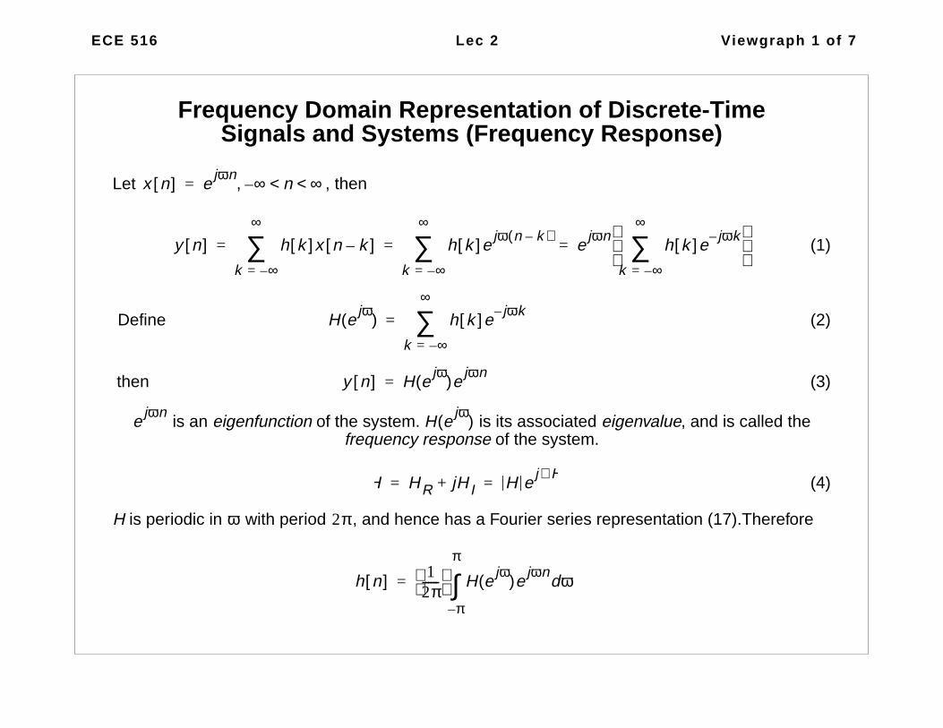
Frequency Domain Representation of Discrete-TimeSignals and Systems (Frequency Response)

Let , then

(1)

Define (2)

then (3)

is an eigenfunction of the system. is its associated eigenvalue, and is called thefrequency response of the system.

(4)

H is periodic in with period , and hence has a Fourier series representation (17).Therefore

x n[ ] ejωn ∞– n ∞< <,=

y n[ ] h k[ ]x n k–[ ]k ∞–=

∞

∑ h k[ ]ejω n k–( )

k ∞–=

∞

∑ ejωn

h k[ ]e jωk–

k ∞–=

∞

∑

= = =

H ejω

( ) h k[ ]e jωk–

k ∞–=

∞

∑=

y n[ ] H ejω

( )ejωn

=

ejωn

H ejω

( )

H HR jHI+ H ej H∠

= =

ω 2π

h n[ ] 12π------

H ejω

( )ejωn

dωπ–

π

∫=


Representation of Sequences by Fourier Transforms:

Any sequence, with suitable convergence conditions:

Inverse Fourier Transform , (5)

Fourier Transform (6)

Frequency Response:

From convolution (15), , Fourier transform of output is

=

(7)

x n[ ] 12π------

X ejω

( )ejωn

dωπ–

π

∫=

X ejω

( ) x k[ ]e jωk–

k ∞–=

∞

∑=

y n[ ] x k[ ]h n k–[ ]k ∞–=∞∑=

Y ejω

( ) y n[ ]e jωn–

n ∞–=

∞

∑ h n k–[ ]x k[ ]e jωn–

k∑

n∑ x k[ ] h n k–[ ]e jωn–

n∑

k∑= = =

x k[ ]e jωk–h n k–[ ]e jω n k–( )–

n∑

k∑ X e

jω( )H e

jω( )=


Symmetry Properties of the Fourier Transform:

Let , where

(8)

x n[ ] x e n[ ] x o n[ ]+=

x e n[ ] 12--- x n[ ] x∗ n–[ ]+( ) x o n[ ], 1

2--- x n[ ] x∗ n–[ ]–( )= =


Fourier Transform Theorems:

TABLE 1. Fourier Transform Theorems

Sequence Theorem Fourier Transform

Linearity

Time Shift

Frequency Shift

Time Reversal , if real x then

Differentiation in Frequency

Convolution

Modulation or Windowing

Parsevals Theorem

,

ax by+ aX bY+

x n nd–[ ] ejωnd–

X ejω( )

ej ω0nx n[ ] X e

j ω ω0–( )( )

x n–[ ] X e jω–( ) X∗ ejω( )

nx n[ ] j ωdd

X ejω( )

x ∗y XY

xy 12π------ X e jθ( )Y e j ω θ–( )( )dθ

π–

π

∫

x n[ ] 2

n ∞–=

∞

∑ 12π------ X e jω( )

2dω

π–

π

∫= x n[ ]y∗ n[ ]n ∞–=

∞

∑ 12π------ X ejω( )Y ∗ ejω( )dω

π–

π

∫=


Linear Constant-Coefficient Difference Equations

Nth-order linear constant-coefficient difference equation

(9)

(10)

Let a0 = 1. Causality, initial conditions, stability, IIR and FIR filters ...

If , then FIR filter, otherwise IIR.

ak y n k–[ ]k 0=

N

∑ br x n r–[ ]r 0=

M

∑=

y n[ ]aka0------y n k–[ ]

k 1=

N

∑–bra0------x n r–[ ]

r 0=

M

∑+=

ai 0 i, 1 2 … N, , ,= =



Averaging Filter

, (11)

=

(12)


(13)

(14)

y n[ ] 1N---- x n r–[ ]

r 0=

N 1–

∑= h n[ ]1N---- 0 n N 1–≤ ≤, ,

0 else,

=

H ejω

( ) h n[ ]e jωn–

n ∞–=

∞

∑ 1N----

ejωn–

n 0=

N 1–

∑ 1N----

1 ejωN–

–

1 ejω–

–-------------------------

= = =

1N----

ωN2

--------- sin

ω2----

sin----------------------e

j N 1–( )ω2----–

H ejω

( )1, ω ωc,≤

0, ωc ω π< <

=

h n[ ] 12π------ 1e

jωndω

ωc–

ωc

∫ωcnsin

πn-------------------= =


Digital Interpolator

(15)

(16)

(17)

H ejω

( ) ejωτ–

h n[ ]e jωn–∑ 0 τ 1< <,= =

h n[ ] 12π------

H ejω

( )ejωn

dωπ–

π

∫=

h n[ ] π n τ–( )sinπ n τ–( )-----------------------------

πτsinπ n τ–( )-------------------- 1–( )n 1+ πτsin

πτ n τ⁄ 1–( )------------------------------ 1–( )= = =n 1+


Sampling of Continuous-Time Signals

Periodic (uniform) Sampling:

(1)

Sampling Frequency: (2)

(3)

(4)

= (5)

(6)

Let , then

x n[ ] x c nT( ) ∞– n ∞< <,=

f s 1 T⁄=

c t( ) X c jΩ( )ejΩt

dΩ∞–

∞

∫ X c jΩ( ) x c t( )ejΩt–

d

∞–

∞

∫=,=

x n[ ] 12π------ X e

jω( )e

jωndω

π–

π

∫ X ejω

( ) x k[ ]e jωk–

k ∞–=

∞

∑=,=

x n[ ] x c nT( ) X c jΩ( )ejΩnT

dΩ∞–

∞

∫ X c jΩ( )ejΩnT

dΩ2r 1–( ) π T⁄( )2r 1+( ) π T⁄( )∫

r ∞–=

∞

∑= = =

12π------ X c jΩ j 2πr

T---------+( )e

jΩnTe

j 2πrndΩπ T⁄–

π T⁄∫r ∞–=

∞

∑ 12π------ X c jΩ j 2πr

T---------+( )

r ∞–=

∞

∑ ejΩnT

dΩπ T⁄–

π T⁄

∫=

Ω ωT----=


(7)

(8)

Nyquist Sampling Theorem:

If is bandlimited with for , then is uniquely determined by itssamples if .

x n[ ] 12π------

1T---- X c

jωT------ j 2πr

T---------+( )

r ∞–=

∞

∑ ejωn

dωπ–

π

∫=

X ejω

( )1T---- X c

jωT------ j 2πr

T---------+( )

r ∞–=

∞

∑=

x c t( ) X c jΩ( ) 0= Ω ΩN> x c t( )x n[ ] x c nT( ) n 0 1± 2± …, , , ,=,= Ωs 2π( ) T⁄ 2ΩN>=


Reconstruction of a Bandlimited Signal from its Samples:

(9)

If , and for , then .

Interpolation,

Digital Interpolator

(10)

(11)

(12)

x r t( ) x n[ ] ct nT–

T----------------( )sin∑ c x( )sin πxsin

πx--------------=,=

x n[ ] x c nT( )= X c jΩ( ) 0= Ω ΩN> x r t( ) x c t( )=

H ejω

( ) ejωτ–

h n[ ]e jωn–∑ 0 τ 1< <,= =

h n[ ] 12π------

H ejω

( )ejωn

dωπ–

π

∫=

h n[ ] π n τ–( )sinπ n τ–( )-----------------------------

πτsinπ n τ–( )-------------------- 1–( )n 1+ πτsin

πτ n τ⁄ 1–( )------------------------------ 1–( )= = =n 1+


Non-Ideal Sampling:

Example, averaging window:

(13)

Let (14)

Then (15)

Let , then (16)

where , Group delay (17)

x n[ ] 1τ--- x c t( )dt

nT τ–( )

nT

∫=

r τ t( )1 τ⁄ 0 t≤ τ< ,,

0 else

=

x n[ ] r τ nT ζ–( )x c ζ( )dζ∞–

∞

∫=

x c t( ) r t ζ–( )x c ζ( )dζ∞–

t

∫ ,= X c jΩ( ) Rτ jΩ( )X c jΩ( )=

Rτ jΩ( )

Ωτ2

-------sin

Ωτ2

-----------------------e

j Ωτ2

-------–= τ 2⁄


Discrete-Time Processing of Continuous-Time Signals:

If is bandlimited, and the sampling rate is above the Nyquist rate, then

(18)



(19)

(20)

If input is samples of bandlimited signal, sampled above Nyquist rate, then after ideal D/A, system

behaves as (21)

Ideal Bandlimited Differentiator

X c jΩ( )

r jΩ( ) Heff jΩ( )X c jΩ( ) Heff jΩ( )H e

jΩ( ) Ω π T⁄< ,,

0, Ω π T⁄≥

=,=

H ejω

( )1, ω ωc,≤

0, ωc ω π< <

=

h n[ ] 12π------ 1e

jωndω

ωc–

ωc

∫ωcnsin

πn-------------------= =

Heff jΩ( )1 ΩT ωc< or Ω ωc T⁄<, ,,

0, ΩT ωc> or Ω ωc T⁄>, ,

=


Impulse Invariance:

Given which is bandlimited, then to choose such that :

, (22)

with the further requirement that T is chosen such that .Then, , or impulse invariance. If is not bandlimited, then

(23)

Frequency Scaling:

Hc jΩ( ) H ejω

( ) Heff jΩ( ) Hc jΩ( )=

H ejω

( ) HcjωT------( ) ω π<,=

Hc jΩ( ) 0 Ω π T⁄≥,=

h n[ ] T hc nT( )= Hc jΩ( )

H ejω

( ) HcjωT------ j 2πr

T---------+( )

r ∞–=

∞

∑=


The z-Transform

(24)

Let , (25)

This is the Fourier transform of . Uniform convergence requires absolute summability. thishappens generally for .

X z( ) x n[ ]z n–

n ∞–=

∞

∑=

z r ejω

= X r ejω

( ) x n[ ]r n–( )e jωn–

n ∞–=

∞

∑=

x n[ ]r n–

R z R< <- +


The z-Transform

(1)

Let , (2)

This is the Fourier transform of . Uniform convergence requires absolute summability. For

, this happens for .

Replacing by in results in the Fourier transform of , provided the unit circle is inthe region of convergence of the z-transform.

X z( ) x n[ ]z n–

n ∞–=

∞

∑=

z r ejω

= X r ejω

( ) x n[ ]r n–( )e jωn–

n ∞–=

∞

∑=

x n[ ]r n–

x n[ ]r n–

n ∞–=

∞

∑ ∞< R z R< <- +

z ejω

X z( ) x n[ ]


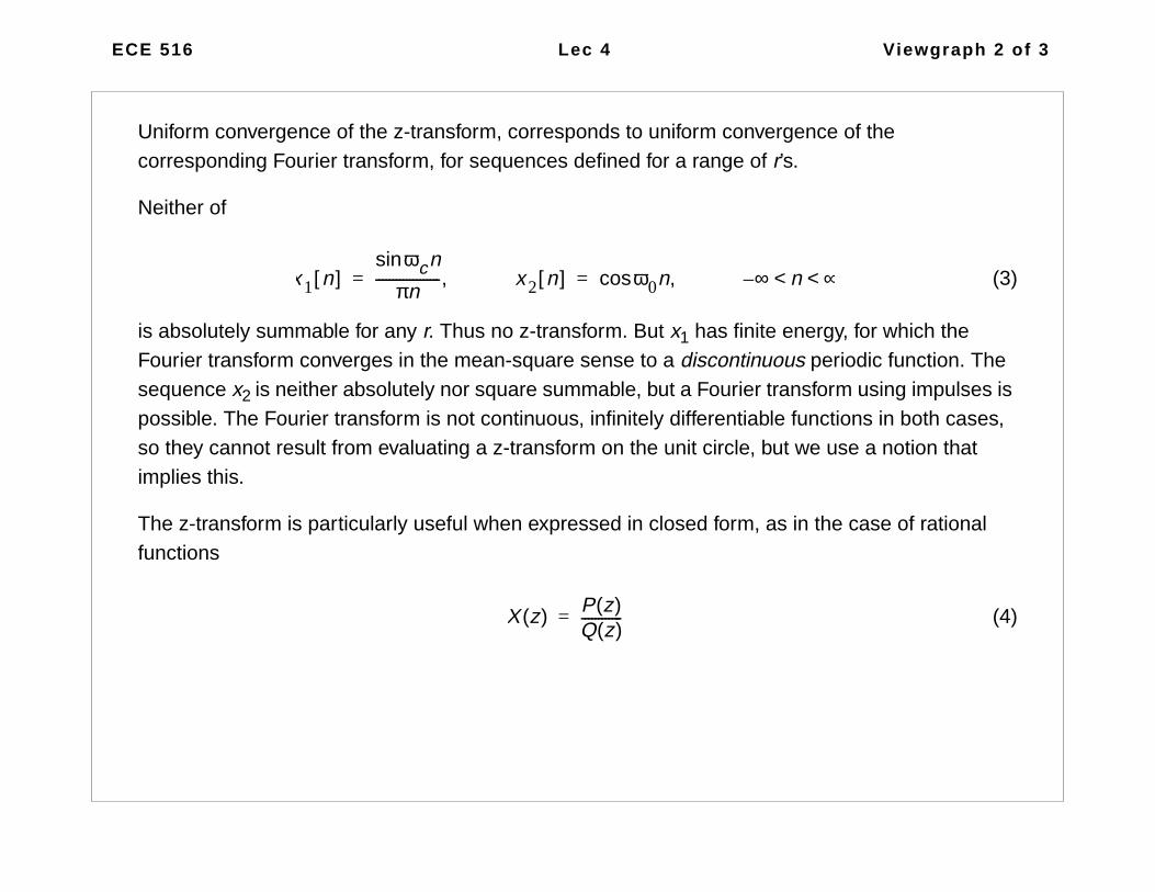
Uniform convergence of the z-transform, corresponds to uniform convergence of thecorresponding Fourier transform, for sequences defined for a range of r’s.

Neither of

(3)

is absolutely summable for any r. Thus no z-transform. But x1 has finite energy, for which theFourier transform converges in the mean-square sense to a discontinuous periodic function. Thesequence x2 is neither absolutely nor square summable, but a Fourier transform using impulses ispossible. The Fourier transform is not continuous, infinitely differentiable functions in both cases,so they cannot result from evaluating a z-transform on the unit circle, but we use a notion thatimplies this.

The z-transform is particularly useful when expressed in closed form, as in the case of rationalfunctions

(4)

x 1 n[ ]ωcnsin

πn------------------- x 2 n[ ] ω0ncos ∞– n ∞< <,=,=

X z( ) P z( )Q z( )------------=


Examples:

exponential and unit step:

(5)

Convergence requires , which is true for ,or .

In region of convergence

(6)

The z- transform converges for any finite value of a, the fourier transform only for |a|<1.

For a = 1, x[n] is unit step sequence with z-transform

(7)

x n[ ] anu n[ ] X z( ) a

nu n[ ]z n–

n ∞–=

∞

∑ az1–( )

n

n 0=

∞

∑= =,=

az1– n

n 0=

∞

∑ ∞< az1–

1< z a>

X z( ) 1

1 az1–

–---------------------

zz a–------------ z a>,= =

X z( )1

1 z1–

–------------------ z 1>,=


Digital Filter Structures

Let

(1)

(2)

y n[ ] ak y n k–[ ]k 1=

N

∑ br x n r–[ ]r 0=

M

∑+=

H z( )

bk zk–

k 0=

M

∑

1 ak zk–

k 1=

N

∑–

--------------------------------------Y z( )X z( )------------= =


State Space Representation

Let M=N (discussion), express in powers of z, and isolate direct coupling:

(3)

Let state variable be the vector of dimension N. Then state space representation

(4)

(5)

(6)

H z( ) d

βk zN 1– k–

k 0=

N 1–

∑

zN αk z

N k–

k 1=

N

∑+

--------------------------------------------------+=

v n( )

v n 1+( ) Av n( ) bx n( )+ ,=

y n( ) cv n( ) d x n( )+=

A

0 1 0 … 0

0 0 1 … 0

0 0 … 0 1

αN– αN 1–– … α1–

b,

0

0

0

1

c, βN 1– βN 2– … β0= = =

H z( ) c zI A–( ) 1–b d+=


(7)

Non-singular Transformations

(8)

Input and output invariant, but

(9)

By changing T, new strauctures are obtained that have different computational, roundoff, andcoefficient sensitivity properties. Changing T results in changing the basis in the state vectorspace in which the system is represented.

h n[ ] cAn 1–

b n, 1 2 …, ,=

d n, 0=

=

Tv n 1+( ) TAT1–Tv n( ) Tbx n( )+ ,=

y n( ) cT1Tv n( ) d x n( )+=

v Tv=

A TAT1–

=

c cT1–

=

b Tb=


The Discrete Fourier Transform

(1)

(2)

x n[ ] 1N---- X k( )e

j 2πN------nk

k 0=

N 1–

∑ ,=

X k( ) x n[ ]ej 2πN------nk–

n 0=

N 1–

∑ ,=

2π/N

WN

z plane

.

W N ej 2πN------–

=


Finite and Periodic Sequences:

(3)

(4)

(5)

(6)

(7)

X z( ) x n[ ]z n–

n 0=

N 1–

∑=

X ejω

( ) x n[ ]e jωn–

n 0=

N 1–

∑ ω, 2πN------k k, 0 1 … N 1.–, , ,= = =

X k( ) X ej 2πN------k

( )≡ x n[ ]ej 2πN------nk–

n 0=

N 1–

∑ k, 0 1 … N 1–, , ,= =

X k( ) X ej 2πN------k

( )≡ x n[ ]W Nnk

n 0=

N 1–

∑ k, 0 1 … N 1–, , ,= =

x n[ ] 1N---- X k( )W

nk–

k 0=

N 1–

∑ n, 0 1 … N 1.–, , ,= =


Constructing from Frequency Samples for Finite Sequences:

(8)

(9)

Infinite Sequences:

(10)

Let

(11)

The inverse DFT of is , defined by ,resulting in

X z( )

X z( ) x n[ ]z n–

n 0=

N 1–

∑ 1N---- X k( )W

nk–

k 0=

N 1–

∑

zn–

n 0=

N 1–

∑= =

1N---- X k( ) W N

k–z

1–( )n

n 0=

N 1–

∑k 0=

N 1–

∑ 1N---- X k( )

1 zN–

–

1 W Nk–

z1–

–------------------------------

k 0=

N 1–

∑ 1 zN–

–N

-------------------X k( )

1 W Nk–

z1–

–------------------------------

k 0=

N 1–

∑= = =

X z( ) x n[ ]z n–

n ∞–=

∞

∑=

X k( ) X z( )

z ej 2π

N------k

=

≡ x n[ ]W Nkn

n ∞–=

∞

∑ k, 0 1 …N 1–, ,= =

X k( ) x n[ ] x n[ ] 1N---- X k( )W

nk–

k 0=

N 1–

∑ n, 0 1 … N 1.–, , ,= =


(12)

Using , as shown

then

(13)

So, is an aliased version of .

Properties of the DFS/DFT:

Linearity: .

Both x1 and x2 are periodic of same period, or finite of same length.

Circular Shift:

Circular (Periodic) Convolution:

x n[ ] 1N---- X k( )W

nk–

k 0=

N 1–

∑ 1N---- x m[ ]W N

kmW N

kn–

m ∞–=

∞

∑k 0=

N 1–

∑ x m[ ] 1N---- W N

k n m )–(–

k 0=

N 1–

∑

m ∞–=

∞

∑= = =

1N---- W N

k n m )–(–

k 0=

N 1–

∑ 1 m, n rN+=

0 else,=

1N---- W N

ks–

k 0=

N 1–

∑1 s, rN=

0 otherwise,

=

for s rN 1N---- W N

ks–

k 0=

N 1–

∑;≠ 1N----

1 W NsN–

–

1 W Ns–

–------------------------ 0= =

1=

1≠

x n[ ] x n rN+[ ]r ∞–=

∞

∑=

x x

x 3 n[ ] ax 1 n[ ] bx 2 n[ ]+ X 3 k( )⇔ aX 1 k( ) bX 2 k( )+= =

x 1 n[ ] x n m+[ ]= ⇔ X 1 k( ) W Nkm–

X k( )=


(14)

(15)

Parseval’s Relation for the DFT:

(16)

Linear Convolution Using the DFT:

Let be of length L, of length M. Then is of length . Padeach of and with zeros so that each is of length . Compute DFT’s,multiply point wise, IDFT and keep only .

If one of the sequences is very long, it is decomposed into sections of appropriate size, convolved,and the partial results combined according to one of the following two schemes:

Overlap-add:

Overlap-save:

x 3 n[ ] x 1 m[ ]x 2 n m–[ ]m 0=

N 1–

∑ X 3 k( )⇔ X 1 k( )X 2 k( )= =

x 3 n[ ] x 1 n[ ]x 2 n[ ] X 3 k( )⇔ 1N---- X 1 r( )X 2 k r–( )

r 0=

N 1–

∑= =

x n[ ] 2

n 0=

N 1–

∑ 1N---- X k( )

2

k 0=

N 1–

∑=

x 1 n[ ] x 2 n[ ] x 3 x 1 x 2= ∗ L M 1–+

x 1 n[ ] x 2 n[ ] N L M 1–+≥L M 1–+


Computation of the DFT

Divide and Conquer Algorithms:

Matrix Multiplication:

Strassen Algorithm: , all . Let n be even for the next step, power of two forthe complete algorithm.

The first step is to divide each matrix into four matrices as follows.

(1)

Instead of the eight matrix multiplications, and four matrix additions needed in directcomputation of the entries of C, the following seven products are computed.

(2)

A B× C= n n× n 2s

=

n2---

n2---×

A11 A12

A21 A22

B11 B12

B21 B22

C11 C12

C21 C22

=

n2---

n2---×

P1 A11 A22+( ) B11 B22+( )=

P2 A21 A22+( )B11=

P3 A11 B12 B22–( )=

P4 A22 B21 B11–( )=

P5 A11 A12+( )B22=

P6 A21 A11–( ) B11 B12+( )=

P7 A12 A22–( ) B21 B22+( )=


Then C is computed in terms of additions of the P’s.

(3)

Instead of 8 multiplications and 4 additions of , the algorithm requires 7 multiplications,and18 additions of matrices. Since multiplication of matrices requires scalarmultiplications, and scalar additions, removing one matrix multiplications at the cost ofadding several matrix additions results in computation reduction for sufficiently large m.

So far we have applied divide and conquer only once. If the rest of the computation of thesubmatrices is done by direct approach, and if we count a scalar multiply as approximately ascostly as a scalar add, as is the case in floating point arithmetic, then the break even point is for

, and the savings approach 1/8 of the regular approach as n increases. But we can applythe algorithm again and again to all the resulting submatrices as long as this results in savings.

If the algorithm is applied repeatedly until computation is completed, then the number ofmultiplications and additions needed to compute the multiplication of matrices, and

respectively, satisfy

C11 A11B11 A12B21+ P1 P4 P5– P7+ += =

C21 A21B11 A22B21+ P2 P4+= =

C12 A11B12 A12B22+ P3 P5+= =

C11 A21B12 A22B22+ P1 P3 P2– P6+ += =

n2---

n2---×

n2---

n2---× m m× m

3

m3

m2

–

n 30=

2r

2r× M r( )

A r( )


(4)

which has the solution, for

(5)

Polynomial Multiplication:

Let and be polynomials of degree n-1 each, where .

(6)

M r 1+( ) 7M r( ) M 0( ), 1,= =

A r 1+( ) 7A r( ) 18 4r×+ A 0( ), 0= =

n 2s

=

M s( ) 7s

272log

( )s

n72log

n2.807,≈= = =

A s( ) 6 7s

4s

–( ) 6 n72log

n2

–( )= =

Pn Qn n 2s

=

Pn x( )Qn x( ) p0 p1x p2x2 … pn 1– x

n 1–+ + + +( ) q0 q1x q2x

2 … qn 1– xn 1–

+ + + +( )= =


Now the trick is to compute , andrecognize that

p0 p1x p2x2 … pn

2--- 1–

x

n2--- 1–

+ + + +

x

n2---

pn2---

pn2--- 1+

x pn2--- 2+

x2 … pn 1– x

n2--- 1–

+ + + +

+

q0 q1x q2x2 … qn

2--- 1–

x

n2--- 1–

+ + + +

x

n2---

qn2---

qn2--- 1+

x qn2--- 2+

x2 … qn 1– x

n2--- 1–

+ + + +

+

Pn2--- 1,

x

n2---

Pn2--- 2,

+

Qn2--- 1,

x

n2---

Qn2--- 2,

+

=

Pn2--- 1,

Qn2--- 1,

x

n2---

Pn2--- 1,

Qn2--- 2,

Pn2--- 2,

Qn2--- 1,

+

xnPn

2--- 2,

Qn2--- 2,

+ +=

Pn2--- 1,

Qn2--- 1,

Pn2--- 2,

Qn2--- 2,

Qn2--- 1,

Qn2--- 2,

–

Pn2--- 2,

Pn2--- 1,

–

, , ,


So, direct computation results in 4 multiplications and one additions of polynomials of degree. With algorithm, 3 multiplications and 4 additions. Repeated application results in

multiplications, and additions.

Decimation-in-Time FFT:

(7)

Let , and notice that implies

.

Pn2--- 1,

Qn2--- 2,

Pn2--- 2,

Qn2--- 1,

+ Qn2--- 1,

Qn2--- 2,

–

Pn2--- 2,

Pn2--- 1,

–

Pn2--- 1,

Qn2--- 1,

Pn2--- 2,

Qn2--- 2,

+ +=

n2--- 1–

3n32log

n1.58≈ 24n

32log

X k( ) X ej 2πN------k

( )≡ x n[ ]W Nnk

n 0=

N 1–

∑ k, 0 1 … N 1–, , ,= =

N 2γ

= W N ej 2πN------–

=

W N0

1 W N

N2----

, 1– W N

N4----

, j– W N

3N4

--------, j W N

r, W N ⁄= = = = =


By separating the data at even and odd time indices, (decimation in time), we obtain

(8)

(9)

. (10)

One N point DFT is replaced by two, N/2 point DFT’s at the cost of N multiplications, and Nadditions. So the number of either additions or multiplications for a DFT of length satisfies

(11)

Let , then

(12)

Which has the solution

(13)

X k( ) x n[ ]W Nnk

n even∑ x n[ ]W N

nk

n odd∑+=

X k( ) x 2r[ ] W N2( )

rk

r 0=

N 2⁄ 1–

∑ W Nk

x 2r 1+[ ] W N2( )

rk

r 0=

N 2⁄ 1–

∑+ W N2, W N 2⁄= =

X k( ) G k( ) W Nk

H k( )+ k, 0 1 … N 1–, , ,= =

N/2 point DFT’s

2i

C 2i

( ) 2C 2i 1–

( ) 2i

+=

C 2i

( ) Ai=

Ai 2Ai 1– 2i

+ A0, 0= =

Aγ 2γA0 γ 2

γ+ N N2log= =


.....

.....

N/2

N/2

G(1)G(G(0)

G(2)G(3)

H(0)H(0)H(1)H(2)H(3)

X(0)X(1)X(2)X(3)

X(4)X(5)X(6)X(7)

x[0]x[2]x[4]x[6]

x[1]x[3]x[5]x[7]

W0N

W1N

WN7

N


Multidimensional Signals and DFT:

Impulse response .

N-Dimensional convolution:

(14)

(15)

(16)

(17)

n-dimensional DFT of finite “length” signal is sampling of n-D F.T.

(18)

Many 1-D DFT’s.

h k 1 k 2 … k n, , ,[ ]

y k 1 k 2 … k n, , ,[ ] … h k 1 l1– k 2 l2– … k n ln–, , ,[ ]x l1 l2 … l n, , ,[ ]l n

∑l 2

∑l 1

∑=

y k( ) x k( ) h k( )= *

Y z1 z2 … zn, , ,( ) X z1 z2 … zn, , ,( )H z1 z2 … zn, , ,( )=

X z1 z2 … zn, , ,( ) … x k 1 k 2 … k n, , ,[ ]z1k 1–

z2k 2–

…znk n–

k n

∑k 2

∑k 1

∑=

X ej ω1 e

j ω2 … ej ωn, , ,( ) … x k 1 k 2 … k n, , ,[ ]e

j ω1k 1 ω2k 2 … ωnk n+ + +( )–

k n

∑k 2

∑k 1

∑=

X l1 l2 … l n, , ,( ) … x k 1 k 2 … k n, , ,[ ]ej 2π

l 1k 1

N 1----------

l 2k 2

N 2---------- …

l nk n

Nn----------+ + +

–

k n 0=

Nn 1–

∑k 2 0=

N 2 1–

∑k 1 0=

N 1 1–

∑=


1-D FFT Derivation in Multidimensional Framework:

(19)

Let , and use , then

(20)

Now define the LxM arrays , then the 1-D DFT isequivalent to:

1- M, L-point DFT’s along 1st dimension of .

2- Multiplication of result of step 1 by .

3- L, M-point DFT’s along 2nd dimension to finally obtain .

For , the cost is . For radix-2 FFT,this becomes

X k( ) X ej 2πN------k

( )≡ x n[ ]ej 2πN------nk–

n 0=

N 1–

∑ k, 0 1 … N 1–, , ,= =

N LM= k l1 Ll2+( ) l1; 0 1 … L 1 l2;–, , , 0 1 … M 1.–, , ,= = =

X l1 Ll2+( ) ej 2πM------k 2l 2–

ej 2πN------k 2l 1–

x M k 1 k 2+[ ]ej 2π

L------k 1l 1–

k 1 0=

L 1–

∑

k 2 0=

M 1–

∑=

x k 1 k 2,[ ] x M k 1 k 2+[ ] X l1 l2,( ); X l1 Ll2+( )= =

x k 1 k 2,[ ]

ej 2πN------l 1k 2–

l1, 0 1 …L 1– k 2, , , 0 1 … M 1–, , ,= =

X l1 l2,( )

N N1 N2 … Nn×××= C N( ) N Ni⁄( )C Ni( ) n 1–( )N+i 1=n∑=

C 2n

( ) n2n 1–

C 2( ) n 1–( )2n+ N N2log

NC 2( )2

---------------- N2log N–+ N N2log≈= =


Filter Design Techniques

Design of Discrete-Time IIR Filters from Continuous-Time Filters:

Bilinear Transformarion:

(1)

(2)

(3)

Imaginary axis in s-plane maps onto unit circle in z-plane, left half plane onto unit disk.

Due to nonlinearity of map:

1- only for filters with piecewise constant magnitude response.

2- phase response is not critical.

s 21 z

1––

1 z1–

+------------------

=

z1 s

2---+

1 s2---–

------------=

Ω 2 ω 2⁄( )tan=


Given the specifications of the desired , the specifications are mapped onto those of ,which is then designed as a continuous-time filter, and then transformed via bilineartransformation into desired digital filter.

Butterworth Filters:

Chebyshev Filters:

Elliptic Filters:

(4)

(5)

H z( ) Hc s( )

Chebyshev Polynomials

-1 -0.5 0.5 1

-1

1

2

3

4

T n x( ) for n 2 4 10, ,= .

T n x( ) n x1–

cos( )cos=

T 0 x( ) 1 T 1 x( ), x T 2 x( ), 2x2

1– T 3 x( ), 4x3

3x– T 4 x( ), 8x4

8x2

– 1+= = = = =


Relative Order of Digital Filters:

(6)

Let , then

(7)

(8)

(9)

(10)

NFIR

10 δ10 1δ2log– 15–

14∆F------------------------------------------------ 1+≈

δ1 δ2 δ= =

NFIR20 δlog– 7.95–

14.36∆F-------------------------------------- 3.8

δelog

∆ω--------------–≈ ≈

nB 1.5δelog

∆ω--------------–≈

nC 1.06δelog

∆ω--------------–≈

nE 0.3 δe ∆ωeloglog≈


Types of Filters:

Minimum phase, Linear phase, and all pass. section 5.4 to end of Ch. 5.

Powers of z: Effect on impulse, frequency, and pole-zero locations. use in filter design andmultirate filtering.

Numerical Design Methods:

IIR Filters:

Deczky’s Method: section 7.3

FIR Filters:

Windowing: section 7.4, 7.5.

Optimum Aproximation: section 7.6. Best mean-square error is just a rectangular-windowedversion of desired impulse response. Best min-max design (equiripple) via Parks-Mclellanalgorithms and the Remez exchange method.


Computationally Efficient Digital Filter Structures

Structures Based on Periodicities and z-Powers:

Periodicities:

MFIR Filters:

Strutures Based on IIR Filters (made to behave as FIR):

MFIR:

Switching and Resetting:

Interpolation:


Computationally Efficient Digital Filter Structures (contd.)

Discussion of papers:

[1] T. Saramaki, and A. Fam, “Subfilter Approach for Designing Computationally Efficient FIR Filters,” ISCAS-88,Espoo, Finland, pp. 2903 -2915, June 7-9, 1988.

[2] Adly T. Fam, “MFIR Filters: Properties and Applications,”IEEE Trans. Acoust., Speech, Signal Processing, vol ASSP-29, pp. 1128-1136, Dec. 1981.

[3] Zhongqi Jing and Adly T. Fam, “A New Structure for Narrow Transition Band, Lowpass Digital Filter Design,”IEEETrans. Acoust., Speech, Signal Processing, vol. ASSP-32, pp. 362-370, Apr. 1984.

[4] A. Fam, “FIR Filters that Approach IIR Filters in their Computational Efficiency,”Twenty-first Annual AsilomarConference on Signals, Systems and Computers, Pacific Grove, California, pp. 28-30, Nov. 2-4, 1987.

[5] Tapio Saramäki and Adly T. Fam, “Properties and Structure of Linear-Phase FIR Filters Based on Switching andResetting of IIR Filters,” ISCAS’90, New Orleans, Louisiana, pp. 3271-3274, May 1-3, 1990.

[6] Chimin Tsai and Adly T. Fam, “Efficient Linear-Phase Filters Based on Switching and Time Reversal,”ISCAS’90, NewOrleans, Louisiana, pp. 2161-2164, May 1-3, 1990.


Optimal Partitioning and Redundancy Removalin Computing Partial Sums

Discussion of concept as introduced in

[1] Adly T. Fam, “Optimal Partitioning and Redundancy Removal in Computing Partial Sums”IEEE Trans. Comput., vol. C-36, pp. 1137- 1143, Oct. 1987.

and related papers, and its applications to FIR filters as in

[2] Adly T. Fam, “Space-Time Duality in Digital Filter Structures,”IEEE Trans. Acoust., Speech, Signal Processing, vol.ASSP-31, pp. 550-556, June 1983.

[3] A. Fam, “A Multi-Signal Bus Architecture for FIR Filters with Single Bit Coefficients,” ICASSP-84, San Diego, CA,pp. 11.11.1-11.11.3, March 19-21, 1984.

ECE 516 ece516TOC.doc Viewgraph

ECE 516: DIGITAL SIGNAL PROCESSING I 1Discrete-Time Signals and Systems 2Linear Discrete-Time Systems 4Frequency Domain Representation of Discrete-TimeSignals and Systems (Frequency Response) 6Linear Constant-Coefficient Difference Equations 8Frequency Domain Representation of Discrete-TimeSignals and Systems (Frequency Response) 10Linear Constant-Coefficient Difference Equations 14Sampling of Continuous-Time Signals 17The z-Transform 23The z-Transform 24Digital Filter Structures 27The Discrete Fourier Transform 30Computation of the DFT 35Filter Design Techniques 44Computationally Efficient Digital Filter Structures 48Computationally Efficient Digital Filter Structures (contd.) 49Optimal Partitioning and Redundancy Removalin Computing Partial Sums 50

discrete-time signals and systems - university at … 516 lec 1 viewgraph 1 of 8 discrete-time...

Documents