discrete probability distributionscathy/math2311/lectures/chapter...discrete probability...

Discrete Probability DistributionsSection 3.1

Cathy Poliak, [email protected]

Office hours: T Th 2:30 - 5:15 pm 620 PGH

Department of MathematicsUniversity of Houston

February 9, 2016

Cathy Poliak, Ph.D. [email protected] Office hours: T Th 2:30 - 5:15 pm 620 PGH (Department of Mathematics University of Houston )Section 3.1 February 9, 2016 1 / 35

Outline

1 Beginning Questions

2 Random Variables

3 Probability Distributions

4 Expected Value

5 Standard Deviation

6 Rules for Means and Variances


Popper Set Up

Fill in all of the proper bubbles.

Use a #2 pencil.

This is popper number 03.


Rules of Probability

1. The probability P(E) of any event E satisfies 0 ≤ P(E) ≤ 1.

2. If S is the sample space in a probability model, then P(S) = 1.

3. Complement rule: For any event E, P(EC) = 1− P(E).

4. General rule for addition: For any two events E and F ,P(E ∪ F ) = P(E) + P(F )− P(E ∩ F ).

5. General rule for multiplication: For any two events E and F ,P(E ∩ F ) = P(E)× P(F |E) or P(E ∩ F ) = P(F )× P(E |F ).

6. Conditional probability: For any two events E and F , P(F, givenE) = P(F |E) = P(F∩E)

P(E) .


Example of Rules

The table below gives the results of a survey of the diet and exercisehabits of 1200 adults:

Diet Don’t diet TotalExercise 315 165 480

Don’t exercise 585 135 720Total 900 300 1200

1. What is the probability that someone in this group exercises?

2. What is the probability that a dieter is also an exerciser?


Random Variables

A random variable is a variable whose value is a numericaloutcome of a random phenomenon.Examples

I X = the sum of two dice, X = 2,3,4, . . . ,12.I X = the number of customers that order a muffin in a coffee shop

between 7:00 am and 9:00 am, X = 0,1, . . ..I X = weight of a box of Lucky Charms, X ≥ 0.

Random variables can either be discrete or continuous.


Discrete random variables

Discrete random variables has either a finite number of valuesor a countable number of values, where countable refers to thefact that there might be infinitely many values, but they result froma counting process.Example of discrete random variable:

I The sum of two dice.I The number of customers who order a muffin in a coffee shop

between 7:00 am and 9:00 am.

The possible values for a discrete random variable has "gaps"between each value.


Continuous random variables

Continuous random variables are random variables that canassume values corresponding to any of the points contained inone or more intervals.Example of continuous random variable:

I The weight of a box of Lucky Charms.

We want to know how both of these types of random variables aredistributed.


Probability Distribution

The probability distribution of a random variable X tells us whatvalues X can take and how to assign probabilities to those values. Thisis the "ideal" distribution for a random variable. Requirements for aprobability distribution:

1. The sum of all the probabilities equal 1.2. The probabilities are between 0 and 1, including 0 and 1.

We will determine the three characteristics of a probability distribution:shape, center, and spread.


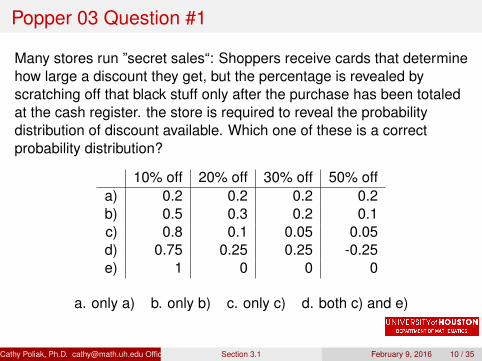
Popper 03 Question #1

Many stores run ”secret sales“: Shoppers receive cards that determinehow large a discount they get, but the percentage is revealed byscratching off that black stuff only after the purchase has been totaledat the cash register. the store is required to reveal the probabilitydistribution of discount available. Which one of these is a correctprobability distribution?

10% off 20% off 30% off 50% offa) 0.2 0.2 0.2 0.2b) 0.5 0.3 0.2 0.1c) 0.8 0.1 0.05 0.05d) 0.75 0.25 0.25 -0.25e) 1 0 0 0

a. only a) b. only b) c. only c) d. both c) and e)


Discrete Probability Distribution

The probability distribution of a discrete random variable X liststhe possible values of X and their probabilities.A probability distribution table of X consists of all possiblevalues of a discrete random variable with thier correspondingprobabilities.


Example of Discrete Probability Distribution

The following is a probability distribution of the number of repairsneeded for a car.

X 0 1 2 3P(X ) 0.72 0.17 0.07 0.04

P(X ≥ 2) = P(X = 2) + P(X = 3) = 0.11P(X > 2) = P(X = 3) = 0.04P(X ≥ 1) = 1− P(X = 0) = 1− 0.72 = 0.28


Popper 03 Questions

Suppose you are given the following probability distribution table.Determine the probabilities below.

X 1 2 3 4 5 6 7P(X ) 0.15 0.05 0.10 ? 0.10 0.15 0.15

2. P(X = 4) a. 0 b. 1 c. 0.7 d. 0.3

3. P(X < 2) a. 0.15 b. 0.20 c. 0.85 d. 0.80

4. P(2 < X ≤ 5) a. 0.05 b. 0.55 c. 0.5 d. 0.2

5. P(X > 3) a. 0.1 b. 0.7 c. 0.8 d. 0.2


Probability Histogram

One way to see the probability distribution of a discrete randomvariable is using a probability histogram. The following is a histogramfor X = the number of repairs needed for a car. What is the "shape" ofthis distribution.

0.10

0.20

0.30

0.40

0.50

0.60

0.70

Probability

0 1 2 3

Number of Repairs

Distributions


Determining Center of a Discrete Random Variable

Suppose that X is a discrete random variable whose distribution is

Values of X x1 x2 x3 · · · xkProbability p1 p2 p3 · · · pk

To find the mean of the random variable X , multiply each possiblevalue by its probability, then add all the products:

µX = E [X ] = x1p1 + x2p2 + x3p3 + · · ·+ xkpk .

This is also called the expected value E [X ].Note: The list here is not a list of observations but a list of all possibleoutcomes. So we are finding µ, the population mean not x̄ , the samplemean.


Example 2 for Expected Value

For the example of the number of repairs for a car.

X P(X ) X × P(X )

0 0.721 0.172 0.073 0.04

Sum =


Popper 03 Question

Let X=The number of traffic accidents daily in a small city. Thefollowing table is the probability distribution for X .

X Probability0 0.101 0.202 0.453 0.154 0.055 0.05

6. Compute the expected number of accidents per day, E [X ].

a. 2.5 b. 2 c. 3 d. 0.1667


Determining the spread of a Discrete Random Variable

The variance of a discrete random variable X is

σ2X = (x1 − µX )2p1 + (x2 − µX )2p2 + · · ·+ (xk − µX )2pk

=k∑

i=1

(xi − µX )2pi

The standard deviation of X is the square root of the variance

σX =√σ2

X .


Easier Calculation for Variance and StandardDeviation from a Discrete Probability Distribution

VAR(X) = σ2x = E(X 2)− [E(X )]2

Where E(X 2) = x21 P(X1) + x2

2 P(X2) + x23 P(X2) + . . .+ x2

n P(Xn).


Example of standard deviation

Determine the standard deviation for the number of repairs needed fora car using the following probability distribution.

X P(X )

0 0.721 0.172 0.073 0.04



Step 1: Determine the mean (expected value) of the probabilitydistribution, µX . µX = E(X ) = 0.43

X P(X )

0 0.721 0.172 0.073 0.04



Step 2: Determine the expected value of X 2.

X P(X ) X 2 X 2 × P(X )

0 0.72 01 0.17 12 0.07 43 0.04 9

E(x2) =



Step 3: Find the variance by taking the difference of the expectedvalue of X 2 and the square of the mean (expected value of X).

VAR(X ) = σ2X = E [X 2]− (E [X ])2 = 0.81− 0.432 = 0.6251

Step 4: Take the square root of the variance. This is the standarddeviation.

SD(X ) = σX =√

0.6251 = 0.70963


Meanings of σX and µX

The mean of the random variable X = number of repairs for avehicle is µX = 0.43 and the standard deviation of X is σX = 0.79.

This implies that the expected number of repairs for a vehicle is0.43 repairs, give or take 0.79 repairs or so.


Popper 03 Question

7. Determine the standard deviation of the number of accidents on agiven day. The expected value is E [X ] = 2.

X 0 1 2 3 4 5P(X ) 0.10 0.20 0.45 0.15 0.05 0.05

a. 19b. 1.4c. 0.2333d. 1.1832


Example

Suppose that in the small city on a given day there was rain. So therewould be at least one accident, the probability distribution of thenumber of accidents will be:

Number of accidents 1 2 3 4 5 6Probability 0.10 0.20 0.45 0.15 0.05 0.05

Compute the mean number of accidents.

Compute the variance of the number of accidents.


Rule 1a for Means and Variances

If X is any random variable and a is a fixed numbers that is addedto all of the values of the random variable thenthe mean increases by that number:

E [a + X ] = a + E [X ].

the variance remains the same:

σ2a+X = σ2

X .

In the example of a rainy day, we added 1 accident to each value,1 + X and the probabilities remained the same.

E [1 + X ] = 1 + E [X ] = 1 + 2 = 3σ2

1+X = σ2X = 1.4


Rule 1b for Means and Variances

If X is any random variable and b is a fixed numbers that ismultiplied to all of the values of the random variable thenthe mean is changed by that multiplier:

E [bX ] = bE [X ].

the variance is also changed by the square of the multiplier:

σ2bX = b2σ2

X .


Playing Roulette

Suppose you play the Roulette wheel in Las Vegas and bet $10 on red.Let X = the amount won, the probability distribution is as follows:

Winnings P(X)10 0.4737-10 0.5263

The expected winnings is µX = −$0.53 with a standard deviation ofσX = $10. Suppose we double the bet to $20. That is 2X , using rule1b determine the following.

1. Calculate the expected winnings, E [2X ].

2. Calculate the variance of the winnings, σ2(2X).

3. Calculate the standard deviation of the winnings, σ(2X).


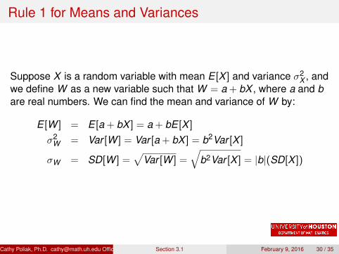
Rule 1 for Means and Variances

Suppose X is a random variable with mean E [X ] and variance σ2X , and

we define W as a new variable such that W = a + bX , where a and bare real numbers. We can find the mean and variance of W by:

E [W ] = E [a + bX ] = a + bE [X ]

σ2W = Var [W ] = Var [a + bX ] = b2Var [X ]

σW = SD[W ] =√

Var [W ] =√

b2Var [X ] = |b|(SD[X ])


#14 from text

Suppose you have a distribution X , with mean = 22 and standarddeviation = 3. Define a new random variable Y = 3X + 1.

1. Find the variance of X .

2. Find the mean of Y .

3. Find the variance of Y .

4. Find the standard deviation of Y .Cathy Poliak, Ph.D. [email protected] Office hours: T Th 2:30 - 5:15 pm 620 PGH (Department of Mathematics University of Houston )Section 3.1 February 9, 2016 31 / 35

Rule 2 for Means

If X and Y are two different random variables, then the mean ofthe sums of the pairs of the random variable is the same as thesum of their means:

E [X + Y ] = E [X ] + E [Y ].

This is called the addition rule for means.The mean of the difference of the pairs of the random variable isthe same as the difference of their means:

E [X − Y ] = E [X ]− E [Y ].


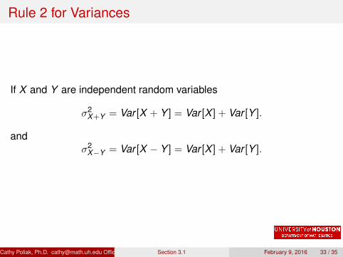
Rule 2 for Variances

If X and Y are independent random variables

σ2X+Y = Var [X + Y ] = Var [X ] + Var [Y ].

andσ2

X−Y = Var [X − Y ] = Var [X ] + Var [Y ].


Example of Rule 2

Tamara and Derek are sales associates in a large electronics andappliance store. The following table shows their mean and standarddeviation of daily sales. Assume that daily sales among the salesassociates are independent.

Sales associate Mean Standard deviationTamara X E [X ] = $1100 σX = $100Derek Y E [Y ] = $1000 σY = $80

1. Determine the mean of the total of Tamara’s and Derek’s dailysales, E [X + Y ].

2. Determine the variance of the total of Tamara’s and Derek’s dailysales, σ2

(X+Y ).

3. Determine the standard deviation of the total of Tamara’s andDerek’s daily sales, σ(X+Y ).


Example


discrete probability distributionscathy/math2311/lectures/chapter...discrete probability...

Documents