discrete mathematics - the archimedeans induction and counting 11 2.1 the pigeonhole principle ......

Discrete Mathematics

Dr. J. Saxl

Michælmas 1995

These notes are maintained by Paul Metcalfe.Comments and corrections to [email protected].

Revision: 2.5Date: 2004/07/26 07:20:10

The following people have maintained these notes.

– date Paul Metcalfe

Contents

Introduction v

1 Integers 11.1 Division . . . . . . . . . . . . . . . . . . . . . . . . . . . . . . . . . 11.2 The division algorithm . . . . . . . . . . . . . . . . . . . . . . . . . 21.3 The Euclidean algorithm . . . . . . . . . . . . . . . . . . . . . . . . 21.4 Applications of the Euclidean algorithm . . . . . . . . . . . . . . . . 4

1.4.1 Continued Fractions . . . . . . . . . . . . . . . . . . . . . . 51.5 Complexity of Euclidean Algorithm . . . . . . . . . . . . . . . . . . 61.6 Prime Numbers . . . . . . . . . . . . . . . . . . . . . . . . . . . . . 6

1.6.1 Uniqueness of prime factorisation . . . . . . . . . . . . . . . 71.7 Applications of prime factorisation . . . . . . . . . . . . . . . . . . . 71.8 Modular Arithmetic . . . . . . . . . . . . . . . . . . . . . . . . . . . 71.9 Solving Congruences . . . . . . . . . . . . . . . . . . . . . . . . . . 8

1.9.1 Systems of congruences . . . . . . . . . . . . . . . . . . . . 91.10 Euler’s Phi Function . . . . . . . . . . . . . . . . . . . . . . . . . . 9

1.10.1 Public Key Cryptography . . . . . . . . . . . . . . . . . . . . 10

2 Induction and Counting 112.1 The Pigeonhole Principle . . . . . . . . . . . . . . . . . . . . . . . . 112.2 Induction . . . . . . . . . . . . . . . . . . . . . . . . . . . . . . . . 112.3 Strong Principle of Mathematical Induction . . . . . . . . . . . . . . 122.4 Recursive Definitions . . . . . . . . . . . . . . . . . . . . . . . . . . 122.5 Selection and Binomial Coefficients . . . . . . . . . . . . . . . . . . 13

2.5.1 Selections . . . . . . . . . . . . . . . . . . . . . . . . . . . . 142.5.2 Some more identities . . . . . . . . . . . . . . . . . . . . . . 14

2.6 Special Sequences of Integers . . . . . . . . . . . . . . . . . . . . . 162.6.1 Stirling numbers of the second kind . . . . . . . . . . . . . . 162.6.2 Generating Functions . . . . . . . . . . . . . . . . . . . . . . 162.6.3 Catalan numbers . . . . . . . . . . . . . . . . . . . . . . . . 172.6.4 Bell numbers . . . . . . . . . . . . . . . . . . . . . . . . . . 182.6.5 Partitions of numbers and Young diagrams . . . . . . . . . . 182.6.6 Generating function for self-conjugate partitions . . . . . . . 20

3 Sets, Functions and Relations 213.1 Sets and indicator functions . . . . . . . . . . . . . . . . . . . . . . . 21

3.1.1 De Morgan’s Laws . . . . . . . . . . . . . . . . . . . . . . . 223.1.2 Inclusion-Exclusion Principle . . . . . . . . . . . . . . . . . 22

iii

iv CONTENTS

3.2 Functions . . . . . . . . . . . . . . . . . . . . . . . . . . . . . . . . 243.3 Permutations . . . . . . . . . . . . . . . . . . . . . . . . . . . . . . 24

3.3.1 Stirling numbers of the first kind . . . . . . . . . . . . . . . . 253.3.2 Transpositions and shuffles . . . . . . . . . . . . . . . . . . . 253.3.3 Order of a permutation . . . . . . . . . . . . . . . . . . . . . 263.3.4 Conjugacy classes in Sn . . . . . . . . . . . . . . . . . . . . 263.3.5 Determinants of an n× n matrix . . . . . . . . . . . . . . . . 26

3.4 Binary Relations . . . . . . . . . . . . . . . . . . . . . . . . . . . . 263.5 Posets . . . . . . . . . . . . . . . . . . . . . . . . . . . . . . . . . . 27

3.5.1 Products of posets . . . . . . . . . . . . . . . . . . . . . . . 283.5.2 Eulerian Digraphs . . . . . . . . . . . . . . . . . . . . . . . 28

3.6 Countability . . . . . . . . . . . . . . . . . . . . . . . . . . . . . . . 283.7 Bigger sets . . . . . . . . . . . . . . . . . . . . . . . . . . . . . . . 30

Introduction

These notes are based on the course “Discrete Mathematics” given by Dr. J. Saxl inCambridge in the Michælmas Term 1995. These typeset notes are totally unconnectedwith Dr. Saxl.

Other sets of notes are available for different courses. At the time of typing thesecourses were:

Probability Discrete MathematicsAnalysis Further AnalysisMethods Quantum MechanicsFluid Dynamics 1 Quadratic MathematicsGeometry Dynamics of D.E.’sFoundations of QM ElectrodynamicsMethods of Math. Phys Fluid Dynamics 2Waves (etc.) Statistical PhysicsGeneral Relativity Dynamical SystemsCombinatorics Bifurcations in Nonlinear Convection

They may be downloaded from

http://www.istari.ucam.org/maths/.

v

http://www.istari.ucam.org/maths/

vi INTRODUCTION

Chapter 1

Integers

Notation. The “natural numbers”, which we will denote by N, are

{1, 2, 3, . . . }.

The integers Z are

{. . . ,−2,−1, 0, 1, 2, . . . }.

We will also use the non-negative integers, denoted either by N0 or Z+, which is N ∪{0}. There are also the rational numbers Q and the real numbers R.

Given a set S, we write x ∈ S if x belongs to S, and x /∈ S otherwise.

There are operations + and · on Z. They have certain “nice” properties which wewill take for granted. There is also “ordering”. N is said to be “well-ordered”, whichmeans that every non-empty subset of N has a least element. The principle of inductionfollows from well-ordering.

Proposition (Principle of Induction). Let P (n) be a statement about n for each n ∈ N.Suppose P (1) is true and P (k) true implies that P (k+1) is true for each k ∈ N. ThenP is true for all n.

Proof. Suppose P is not true for all n. Then consider the subset S of N of all numbersk for which P is false. Then S has a least element l. We know that P (l − 1) is true(since l > 1), so that P (l) must also be true. This is a contradiction and P holds for alln.

1.1 Division

Given two integers a, b ∈ Z, we say that a divides b (and write a | b) if a 6= 0 andb = a · q for some q ∈ Z (a is a divisor of b). a is a proper divisor of b if a is not ±1or ±b.

Note. If a | b and b | c then a | c, for if b = q1a and c = q2b for q1, q2 ∈ Z thenc = (q1 ·q2)a. If d | a and d | b then d | ax+ by. The proof of this is left as an exercise.

1

2 CHAPTER 1. INTEGERS

1.2 The division algorithmLemma 1.1. Given a, b ∈ N there exist unique integers q, r ∈ N with a = qb + r,0 ≤ r < b.

Proof. Take q the largest possible such that qb ≤ a and put r = a−qb. Then 0 ≤ r < bsince a− qb ≥ 0 but (q + 1)b ≥ a. Now suppose that a = q1b + r with q1, r1 ∈ N and0 ≤ r1 < b. Then 0 = (q − q1)b + (r − r1) and b | r − r1. But −b < r − r1 < b sothat r = r1 and hence q = q1.

It is clear that b | a iff r = 0 in the above.

Definition. Given a, b ∈ N then d ∈ N is the highest common factor (greatest commondivisor) of a and b if:

1. d | a and d | b,

2. if d′ | a and d′ | b then d′ | d (d′ ∈ N).

The highest common factor (henceforth hcf) of a and b is written (a, b) or hcf(a, b).The hcf is obviously unique — if c and c′ are both hcf’s then they both divide each

other and are therefore equal.

Theorem 1.1 (Existance of hcf). For a, b ∈ N hcf(a, b) exists. Moreover there existintegers x and y such that (a, b) = ax + by.

Proof. Consider the set I = {ax + by : x, y ∈ Z and ax + by > 0}. Then I 6= ∅ so letd be the least member of I . Now ∃x0, y0 such that d = ax0 + by0, so that if d′ | a andd′ | b then d′ | d.

Now write a = qd + r with q, r ∈ N0, 0 ≤ r < d. We have r = a − qd =a(1−qx0)+b(−qy0). So r = 0, as otherwise r ∈ I: contrary to d minimal. Similiarly,d | b and thus d is the hcf of a and b.

Lemma 1.2. If a, b ∈ N and a = qb + r with q, r ∈ N0 and 0 ≤ r < b then(a, b) = (b, r).

Proof. If c | a and c | b then c | r and thus c | (b, r). In particular, (a, b) | (b, r). Nownote that if c | b and c | r then c | a and thus c | (a, b). Therefore (b, r) | (a, b) andhence (b, r) = (a, b).

1.3 The Euclidean algorithmSuppose we want to find (525, 231). We use lemmas (1.1) and (1.2) to obtain:

525 = 2× 231 + 63231 = 3× 63 + 4263 = 1× 42 + 2142 = 2× 21 + 0

So (525, 231) = (231, 63) = (63, 42) = (42, 21) = 21. In general, to find (a, b):

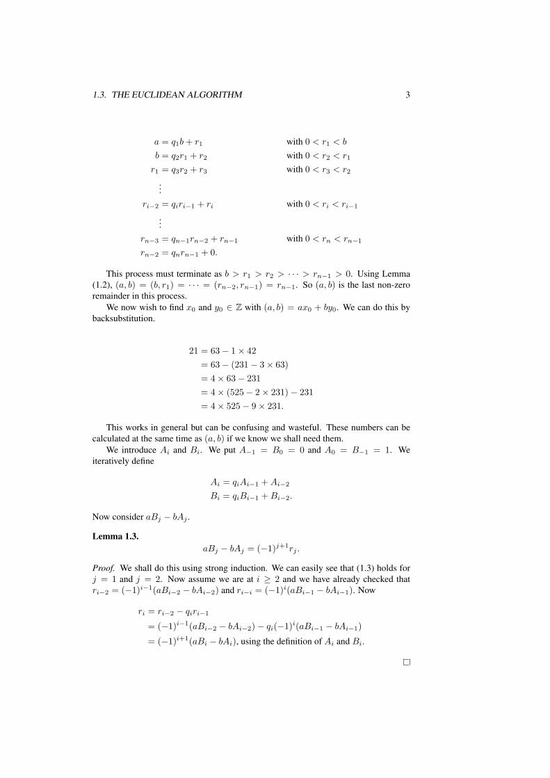
1.3. THE EUCLIDEAN ALGORITHM 3

a = q1b + r1 with 0 < r1 < b

b = q2r1 + r2 with 0 < r2 < r1

r1 = q3r2 + r3 with 0 < r3 < r2

...ri−2 = qiri−1 + ri with 0 < ri < ri−1

...rn−3 = qn−1rn−2 + rn−1 with 0 < rn < rn−1

rn−2 = qnrn−1 + 0.

This process must terminate as b > r1 > r2 > · · · > rn−1 > 0. Using Lemma(1.2), (a, b) = (b, r1) = · · · = (rn−2, rn−1) = rn−1. So (a, b) is the last non-zeroremainder in this process.

We now wish to find x0 and y0 ∈ Z with (a, b) = ax0 + by0. We can do this bybacksubstitution.

21 = 63− 1× 42= 63− (231− 3× 63)= 4× 63− 231= 4× (525− 2× 231)− 231= 4× 525− 9× 231.

This works in general but can be confusing and wasteful. These numbers can becalculated at the same time as (a, b) if we know we shall need them.

We introduce Ai and Bi. We put A−1 = B0 = 0 and A0 = B−1 = 1. Weiteratively define

Ai = qiAi−1 + Ai−2

Bi = qiBi−1 + Bi−2.

Now consider aBj − bAj .

Lemma 1.3.aBj − bAj = (−1)j+1rj .

Proof. We shall do this using strong induction. We can easily see that (1.3) holds forj = 1 and j = 2. Now assume we are at i ≥ 2 and we have already checked thatri−2 = (−1)i−1(aBi−2 − bAi−2) and ri−i = (−1)i(aBi−1 − bAi−1). Now

ri = ri−2 − qiri−1

= (−1)i−1(aBi−2 − bAi−2)− qi(−1)i(aBi−1 − bAi−1)

= (−1)i+1(aBi − bAi), using the definition of Ai and Bi.


Lemma 1.4.AiBi+1 −Ai+1Bi = (−1)i

Proof. This is done by backsubstitution and using the definition of Ai and Bi.

An immediate corollary of this is that (Ai, Bi) = 1.

Lemma 1.5.

An =a

(a, b)Bn =

b

(a, b).

Proof. (1.3) for i = n gives aBn = bAn. Therefore a(a,b)Bn = b

(a,b)An. Now a(a,b)

and b(a,b) are coprime. An and Bn are coprime and thus this lemma is therefore an

immediate consequence of the following theorem.

Theorem 1.2. If d | ce and (c, d) = 1 then d | e.

Proof. Since (c, d) = 1 we can write 1 = cx + dy for some x, y ∈ Z. Then e =ecx + edy and d | e.

Definition. The least common multiple (lcm) of a and b (written [a, b]) is the integer lsuch that

1. a | l and b | l,

2. if a | l′ and b | l′ then l | l′.

It is easy to show that [a, b] = ab(a,b) .

1.4 Applications of the Euclidean algorithm

Take a, b and c ∈ Z. Suppose we want to find all the solutions x, y ∈ Z of ax+by = c.A necessary condition for a solution to exist is that (a, b) | c, so assume this.

Lemma 1.6. If (a, b) | c then ax + by = c has solutions in Z.

Proof. Take x′ and y′ ∈ Z such that ax′ + by′ = (a, b). Then if c = q(a, b) then ifx0 = qx′ and y0 = qy′, ax0 + by0 = c.

Lemma 1.7. Any other solution is of the form x = x0 + bk(a,b) , y = y0 − ak

(a,b) fork ∈ Z.

Proof. These certainly work as solutions. Now suppose x1 and y1 is also a solution.Then a

(a,b) (x0 − x1) = − b(a,b) (y0 − y1). Since a

(a,b) and b(a,b) are coprime we have

a(a,b) | (y0 − y1) and b

(a,b) | (x0 − x1). Say that y1 = y0 − ak(a,b) , k ∈ Z. Then

x1 = x0 + bk(a,b) .

1.4. APPLICATIONS OF THE EUCLIDEAN ALGORITHM 5

1.4.1 Continued FractionsWe return to 525 and 231. Note that

535231

= 2 +63231

= 2 +1

23163

= 2 +1

3 + 4263

= 2 +1

3 + 11+ 1

2

.

Notation.535231

= 2 +1

3+1

1+12

= [2, 3, 1, 2] = 2; 3, 1, 2.

Note that 2, 3, 1 and 2 are just the qi’s in the Euclidean algorithm. The rationalab > 0 is written as a continued fraction

a

b= q1 +

1q2+

1q3+

. . .1qn

,

with all the qi ∈ N0, qi ≥ 1 for 1 < i < n and qn ≥ 2.

Lemma 1.8. Every rational ab with a and b ∈ N has exactly one expression in this

form.

Proof. Existance follows immediately from the Euclidean algorithm. As for unique-ness, suppose that

a

b= p1 +

1p2+

1p3+

. . .1

pm

with the pi’s as before. Firstly p1 = q1 as both are equal to bab c. Since 1

p2+1

...

< 1 then

(a

b− p1

)−1

= p2 +1

p3 + 1...

=(a

b− q1

)−1

= q2 +1

q3 + 1...

.

Thus p2 = q2 and so on.

Now, suppose that given [q1, q2, . . . , qn] we wish to find ab equal to it. Then we

work out the numbers Ai and Bi as in the Euclidean algorithm. Then ab = An

Bnby

lemma (1.3).If we stop doing this after i steps we get Ai

Bi= [q1, q2, . . . , qi]. The numbers Ai

Biare

called the “convergents” to ab .

Using lemma (1.4), we get that Ai

Bi− Ai−1

Bi−1= (−1)i

Bi−1Bi. Now the Bi are strictly

increasing, so the gaps are getting smaller and the signs alternate. We get

A1

B1<

A3

B3< · · · < a

b< · · · < A4

B4<

A2

B2.

The approximations are getting better and better; in fact∣∣∣Ai

Bi− a

b

∣∣∣ ≤ 1BiBi+1

.

∗ — Continued fractions for irrationals

This can also be done for irrationals, but the continued fractions become infinite. Forinstance we can get approximations to π using the calculator. Take the integral part,print, subtract it, invert and repeat. We get π = [3, 7, 15, 1, . . . ]. The convergents are3, 22

7 and 333106 . We are already within 10−4 of π. There is a good approximation as Bi

increases. As an exercise, show that√

2 = [1, 2, 2, 2, . . . ].


1.5 Complexity of Euclidean Algorithm

Given a and b, how many steps does it take to find (a, b). The Euclidean algorithm isgood.

Proposition. The Euclidean algorithm will find (a, b), a > b in fewer than 5d(b) steps,where d(b) is the number of digits of b in base 10.

Proof. We look at the worst case scenario. What are the smallest numbers needing nsteps. In this case qi = 1 for 1 ≤ i < n and qn = 2. Using these qi’s to calculate An

and Bn we find the Fibonacci numbers, that is the numbers such that F1 = F2 = 1,Fi+2 = Fi+1 + Fi. We get An = Fn+2 and Bn = Fn+1. So if b < Fn+1 then fewerthan n steps will do. If b has d digits then

b ≤ 10d − 1 ≤ 1√5

(1 +

√5

2

)5d+2

− 1 < F5d+2,

as

Fn =1√5

[(1 +

√5

2

)n

−

(1−

√5

2

)n]. This will be shown later.

1.6 Prime Numbers

A natural number p is a prime iff p > 1 and p has no proper divisors.

Theorem 1.3. Any natural number n > 1 is a prime or a product of primes.

Proof. If n is a prime then we are finished. If n is not prime then n = n1 · n2 with n1

and n2 proper divisors. Repeat with n1 and n2.

Theorem 1.4 (Euclid). There are infinitely many primes.

Proof. Assume not. Then let p1, p2, . . . , pn be all the primes. Form the number N =p1p2 . . . pn +1. Now N is not divisible by any of the pi — but N must either be primeor a product of primes, giving a contradiction.

This can be made more precise. The following argument of Erdos shows that the kth

smallest prime pk satisfies pk ≤ 4k−1 + 1. Let M be an integer such that all numbers≤ M can be written as the product of the powers of the first k primes. So any suchnumber can be written

m2pi11 pi2

2 . . . pik

k ,

with i1, . . . , ik ∈ {0, 1}. Now m ≤√

M , so there are at most√

M 2k possible num-bers less than M . Hence M ≤ 2k

√M , or M ≤ 4k. Hence pk+1 ≤ 4k + 1.

A much deeper result (which will not be proved in this course!) is the Prime Num-ber Theorem, that pk ∼ k log k.

1.7. APPLICATIONS OF PRIME FACTORISATION 7

1.6.1 Uniqueness of prime factorisationLemma 1.9. If p | ab, a, b ∈ N then p | a and/or p | b.

Proof. If p - a then (p, a) = 1 and so p | b by theorem (1.2).

Theorem 1.5. Every natural number > 1 has a unique expression as the product ofprimes.

Proof. The existence part is theorem (1.3). Now suppose n = p1p2 . . . pk = q1q2 . . . ql

with the pi’s and qj’s primes. Then p1 | q1 . . . ql, so p1 = qj for some j. By renumber-ing (if necessary) we can assume that j = 1. Now repeat with p2 . . . pk and q2 . . . ql,which we know must be equal.

There are perfectly nice algebraic systems where the decomposition into primesis not unique, for instance Z

[√−5]

= {a + b√−5 : a, b ∈ Z}, where 6 = (1 +√

−5)(1 −√−5) = 2 × 3 and 2, 3 and 1 ±

√−5 are each “prime”. Or alternatively,

2Z = {all even numbers}, where “prime” means “not divisible by 4”.

1.7 Applications of prime factorisationLemma 1.10. If n ∈ N is not a square number then

√n is irrational.

Proof. Suppose√

n = ab , with (a, b) = 1. Then nb2 = a2. If b > 1 then let p be a

prime dividing b. Thus p | a2 and so p | a, which is impossible as (a, b) = 1. Thusb = 1 and n = a2.

This lemma can also be stated: “if n ∈ N with√

n ∈ Q then√

n ∈ N”.

Definition. A real number θ is algebraic if it satisfies a polynomial equation withcoefficients in Z.

Real numbers which are not algebraic are transcendental (for instance π and e).Most reals are transcendental.

If the rational ab ( with (a, b) = 1 ) satisfies a polynomial with coefficients in Z

thencnan + cn−1a

n−1b + . . . bnc0 = 0

so b | cn and a | c0. In particular if cn = 1 then b = 1, which is stated as “algebraicintegers which are rational are integers”.

Note that if a = pα11 pα2

2 . . . pαk

k and b = pβ11 pβ2

2 . . . pβk

k with αi, βi ∈ N0 then(a, b) = pγ1

1 pγ22 . . . pγk

k and [a, b] = pδ11 pδ2

2 . . . pδk

k , γi = min{αi, βi} and δi =max{αi, βi}.

Major open problems in the area of prime numbers are the Goldbach conjecture(“every even number greater than two is the sum of two primes”) and the twin primesconjecture (“there are infinitely many prime pairs p and p + 2”).

1.8 Modular ArithmeticDefinition. If a and b ∈ Z, m ∈ N we say that a and b are “congruent mod(ulo) m”if m | a− b. We write a ≡ b (mod m).

It is a bit like = but less restrictive. It has some nice properties:


• a ≡ a (mod m),

• if a ≡ b (mod m) then b ≡ a (mod m),

• if a ≡ b (mod m) and b ≡ c (mod m) then a ≡ c (mod m).

Also, if a1 ≡ b1 (mod m) and a2 ≡ b2 (mod m)

• a1 + a2 ≡ b1 + b2 (mod m),

• a1a2 ≡ b1a2 ≡ b1b2 (mod m).

Lemma 1.11. For a fixed m ∈ N, each integer is congruent to precisely one of theintegers

{0, 1, . . . ,m− 1}.

Proof. Take a ∈ Z. Then a = qm + r for q, r ∈ Z and 0 ≤ r < m. Then a ≡ r(mod m).

If 0 ≤ r1 < r2 < m then 0 < r2 − r1 < m, so m - r2 − r1 and thus r1 6≡ r2

(mod m).

Example. No integer congruent to 3 (mod 4) is the sum of two squares.

Solution. Every integer is congruent to one of 0, 1, 2, 3 (mod 4). The square of anyinteger is congruent to 0 or 1 (mod 4) and the result is immediate.

Similarly, using congruence modulo 8, no integer congruent to 7 (mod 8) is thesum of 3 squares.

1.9 Solving Congruences

We wish to solve equations of the form ax ≡ b (mod m) given a, b ∈ Z and m ∈ Nfor x ∈ Z. We can often simplify these equations, for instance 7x ≡ 3 (mod 5)reduces to x ≡ 4 (mod 5) (since 21 ≡ 1 and 9 ≡ 4 (mod 5)).

This equations are not always soluble, for instance 6x ≡ 4 (mod 9), as 9 - 6x− 4for any x ∈ Z.

How to do it

The equation ax ≡ b (mod m) can have no solutions if (a,m) - b since then m - ax−bfor any x ∈ Z. So assume that (a,m) | b.

We first consider the case (a,m) = 1. Then we can find x0 and y0 ∈ Z suchthat ax0 + my0 = b (use the Euclidean algorithm to get x′ and y′ ∈ Z such thatax′ + my′ = 1). Then put x0 = bx′ so ax0 ≡ b (mod m). Any other solution iscongruent to x0 (mod m), as m | a(x0 − x1) and (a,m) = 1.

So if (a,m) = 1 then a solution exists and is unique modulo m.

1.10. EULER’S PHI FUNCTION 9

1.9.1 Systems of congruencesWe consider the system of equations

x ≡ a mod m

x ≡ b mod n.

Our main tool will be the Chinese Remainder Theorem.

Theorem 1.6 (Chinese Remainder Theorem). Assume m,n ∈ N are coprime and leta, b ∈ Z. Then ∃x0 satisfying simultaneously x0 ≡ a (mod m) and x0 ≡ b (mod n).Moreover the solution is unique up to congruence modulo mn.

Proof. Write cm + dn = 1 with m,n ∈ Z. Then cm is congruent to 0 modulo mand 1 modulo n. Similarly dn is congruent to 1 modulo m and 0 modulo n. Hencex0 = adn + bcm satifies x0 ≡ a (mod m) and x0 ≡ b (mod n). Any other solutionx1 satisfies x0 ≡ x1 both modulo m and modulo n, so that since (m,n) = 1, mn |x0 − x1 and x1 ≡ x0 (mod mn).

Finally, if 1 < (a,m) then replace the congruence with one obtained by dividingby (a,m) — that is consider

a

(a,m)x ≡ b

(a,m)mod

m

(a,m).

Theorem 1.7. If p is a prime then (p− 1)! ≡ −1 (mod p).

Proof. If a ∈ N, a ≤ p − 1 then (a, p) = 1 and there is a unique solution of ax ≡ 1(mod p) with x ∈ N and x ≤ p−1. x is the inverse of a modulo p. Observe that a = xiff a2 ≡ 1 (mod p), iff p | (a + 1)(a− 1), which gives that a = 1 or p− 1. Thereforethe elements in {2, 3, 4, . . . , p − 2} pair off so that 2 × 3 × 4 × · · · × (p − 2) ≡ 1(mod p) and the theorem is proved.

1.10 Euler’s Phi FunctionDefinition. For m ∈ N, define φ(m) to be the number of nonnegative integers lessthan m which are coprime to m.

φ(1) = 1. If p is prime then φ(p) = p− 1 and φ(pa) = pa(1− 1

p

).

Lemma 1.12. If m,n ∈ N with (m,n) = 1 then φ(mn) = φ(m)φ(n). φ is said to bemultiplicative.

Let Um = {x ∈ Z : 0 ≤ x < m, (x,m) = 1, the reduced set of residues or set ofinvertible elements. Note that φ(m) = |Um|.

Proof. If a ∈ Um and b ∈ Un then there exists a unique x ∈ Umn. with c ≡ a(mod m) and c ≡ b (mod n) (by theorem (1.6)). Such a c is prime to mn, since it isprime to m and to n. Conversely, any c ∈ Umn arises in this way, from the a ∈ Um

and b ∈ Un such that a ≡ c (mod m), b ≡ c (mod n). Thus |Umn| = |Um| |Un| asrequired.


An immediate corollary of this is that for any n ∈ N,

φ(n) = n∏p|n

p prime

(1− 1

p

).

Theorem 1.8 (Fermat-Euler Theorem). Take a, m ∈ N such that (a,m) = 1. Thenaφ(m) ≡ 1 (mod m).

Proof. Multiply each residue ri by a and reduce modulo m. The φ(m) numbersthus obtained are prime to m and are all distinct. So the φ(m) new numbers are justr1, . . . , rφ(m) in a different order. Therefore

r1r2 . . . rφ(m) ≡ ar1ar2 . . . arφ(m) (mod m)

≡ aφ(m)r1r2 . . . rφ(m) (mod m).

Since (m, r1r2 . . . rφ(m)) = 1 we can divide to obtain the result.

Corollary (Fermat’s Little Theorem). If p is a prime and a ∈ Z such that p - a thenap−1 ≡ 1 (mod p).

This can also be seen as a consequence of Lagrange’s Theorem, since Um is a groupunder multiplication modulo m.

Fermat’s Little Theorem can be used to check that n ∈ N is prime. If ∃a coprimeto n such that an−1 6≡ 1 (mod n) then n is not prime.

1.10.1 Public Key CryptographyPrivate key cryptosystems rely on keeping the encoding key secret. Once it is knownthe code is not difficult to break. Public key cryptography is different. The encodingkeys are public knowledge but decoding remains “impossible” except to legitimateusers. It is usually based of the immense difficulty of factorising sufficiently largenumbers. At present 150 – 200 digit numbers cannot be factorised in a lifetime.

We will study the RSA system of Rivest, Shamir and Adleson. The user A (forAlice) takes two large primes pA and qA with > 100 digits. She obtains NA = pAqA

and chooses at random ρA such that (ρA, φ(NA)) = 1. We can ensure that pA − 1 andqA − 1 have few factors. Now A publishes the pair NA and ρA.

By some agreed method B (for Bob) codes his message for Alice as a sequence ofnumbers M < NA. Then B sends A the number MρA (mod NA). When Alice wantsto decode the message she chooses dA such that dAρA ≡ 1 (mod φ)(NA). ThenMρAdA ≡ M (mod NA) since Mφ(NA) ≡ 1. No-one else can decode messages toAlice since they would need to factorise NA to obtain φ(NA).

If Alice and Bob want to be sure who is sending them messages, then Bob couldsend Alice EA(DB(M)) and Alice could apply EBDA to get the message — if it’sfrom Bob.

Chapter 2

Induction and Counting

2.1 The Pigeonhole PrincipleProposition (The Pigeonhole Principle). If nm + 1 objects are placed into n boxesthen some box contains more than m objects.

Proof. Assume not. Then each box has at most m objects so the total number of objectsis nm — a contradiction.

A few examples of its use may be helpful.

Example. In a sequence of at least kl+1 distinct numbers there is either an increasingsubsequence of length at least k+1 or a decreasing subsequence of length at least l+1.

Solution. Let the sequence be c1, c2, . . . , ckl+1. For each position let ai be the lengthof the longest increasing subsequence starting with ci. Let dj be the length of thelongest decreasing subsequence starting with cj . If ai ≤ k and di ≤ l then there areonly at most kl distinct pairs (ai, dj). Thus we have ar = as and dr = ds for some1 ≤ r < s ≤ kl + 1. This is impossible, for if cr < cs then ar > as and if cr > cs

then dr > ds. Hence either some ai > k or dj > l.

Example. In a group of 6 people any two are either friends or enemies. Then there areeither 3 mutual friends or 3 mutual enemies.

Solution. Fix a person X . Then X has either 3 friends or 3 enemies. Assume theformer. If a couple of friends of X are friends of each other then we have 3 mutualfriends. Otherwise, X’s 3 friends are mutual enemies.

Dirichlet used the pigeonhole principle to prove that for any irrational α there areinfinitely many rationals p

q satisfying∣∣∣α− p

q

∣∣∣ < 1q2 .

2.2 InductionRecall the well-ordering axiom for N0: that every non-empty subset of N0 has a leastelement. This may be stated equivalently as: “there is no infinite descending chain inN0”. We also recall the (weak) principle of induction from before.

11

12 CHAPTER 2. INDUCTION AND COUNTING

Proposition (Principle of Induction). Let P (n) be a statement about n for each n ∈N0. Suppose P (k0) is true for some k0 ∈ N0 and P (k) true implies that P (k + 1) istrue for each k ∈ N. Then P (n) is true for all n ∈ N0 such that n ≥ k0.

The favourite example is the Tower of Hanoi. We have n rings of increasing radiusand 3 vertical rods (A, B and C) on which the rings fit. The rings are initially stackedin order of size on rod A. The challenge is to move the rings from A to B so that alarger ring is never placed on top of a smaller one.

We write the number of moves required to move n rings as Tn and claim thatTn = 2n− 1 for n ∈ N0. We note that T0 = 0 = 20− 1, so the result is true for n = 0.

We take k > 0 and suppose we have k rings. Now the only way to move the largestring is to move the other k − 1 rings onto C (in Tk−1 moves). We then put the largestring on rod B (in 1 move) and move the k−1 smaller rings on top of it (in Tk−1 movesagain). Assume that Tk−1 = 2k−1 − 1. Then Tk = 2Tk−1 + 1 = 2k − 1. Hence theresult is proven by the principle of induction.

2.3 Strong Principle of Mathematical InductionProposition (Strong Principle of Induction). If P (n) is a statement about n for eachn ∈ N0, P (k0) is true for some k0 ∈ N0 and the truth of P (k) is implied by the truthof P (k0), P (k0 + 1), . . . , P (k− 1) then P (n) is true for all n ∈ N0 such that n ≥ k0.

The proof is more or less as before.

Example (Evolutionary Trees). Every organism can mutate and produce 2 new ver-sions. Then n mutations are required to produce n + 1 end products.

Proof. Let P (n) be the statement “n mutations are required to produce n + 1 endproducts”. P0 is clear. Consider a tree with k + 1 end products. The first mutation (theroot) produces 2 trees, say with k1 + 1 and k2 + 1 end products with k1, k2 < k. Thenk + 1 = k1 + 1 + k2 + 1 so k = k1 + k2 + 1. If both P (k1) and P (k2) are true thenthere are k1 mutations on the left and k2 on the right. So in total we have k1 + k2 + 1mutations in our tree and P (k) is true is P (k1) and P (k2) are true. Hence P (n) is truefor all n ∈ N0.

2.4 Recursive Definitions(Or in other words) Defining f(n), a formula or functions, for all n ∈ N0 with n ≥ k0

by defining f(k0) and then defining for k > k0, f(k) in terms of f(k0), f(k0 + 1),. . . , f(k − 1).

The obvious example is factorials, which can be defined by n! = n(n − 1)! forn ≥ 1 and 0! = 1.

Proposition. The number of ways to order a set of n points is n! for all n ∈ N0.

Proof. This is true for n = 0. So, to order an n-set, choose the 1st element in n waysand then order the remaining n− 1-set in (n− 1)! ways.

Another example is the Ackermann function, which appears on example sheet 2.

2.5. SELECTION AND BINOMIAL COEFFICIENTS 13

2.5 Selection and Binomial CoefficientsWe define a set of polynomials for m ∈ N0 as

xm = x(x− 1)(x− 2) . . . (x−m + 1),

which is pronounced “x to the m falling”. We can do this recursively by x0 = 1 andxm = (x−m + 1)xm−1 for m > 0. We also define “x to the m rising” by

xm = x(x + 1)(x + 2) . . . (x + m− 1).

We further define(

xm

)(read “x choose m”) by(

x

m

)=

xm

m!.

It is also convienient to extend this definition to negative m by(

xm

)= 0 if m < 0,

m ∈ Z. By fiddling a little, we can see that for n ∈ N, n ≥ m(n

m

)=

n!m!(n−m)!

.

Proposition. The number of k-subsets of a given n-set is(nk

).

Proof. We can choose the first element to be included in our k-subset in n ways, thenthen next in n − 1 ways, down to the kth which can be chosen in n − k + 1 ways.However, ordering of the k-subset is not important (at the moment), so divide nk

k! to getthe answer.

Theorem 2.1 (The Binomial Theorem). For a and b ∈ R, n ∈ N0 then

(a + b)n =∑

k

(n

k

)akbn−k.

There are many proofs of this fact. We give one and outline a second.

Proof. (a+b)n = (a+b)(a+b) . . . (a+b), so the coefficient of akbn−k is the numberof k-subsets of an n-set — so the coefficient is

(nk

).

Proof. This can also be done by induction on n, using the fact that(n

k

)=(

n− 1k − 1

)+(

n− 1k

).

There are a few conseqences of the binomial expansion.

1. For m,n ∈ N0 and n ≥ m,(

nm

)∈ N0 so m! divides the product of any m

consecutive integers.

2. Putting a = b = 1 in the binomial theorem gives 2n =∑

k

(nk

)— so the number

of subsets of an n-set is 2n. There are many proofs of this fact. An easy one isby induction on n. Write Sn for the total number of subsets of an n-set. ThenS0 = 1 and for n > 0, Sn = 2Sn−1. (Pick a point in the n-set and observe thatthere are Sn−1 subsets not containing it and Sn−1 subsets containing it.


3. (1 − 1)n = 0 =∑

k

(nk

)(−1)k — so in any finite set the number of subsets of

even sizes equals the number of subsets of odd sizes.

It also gives us another proof of Fermat’s Little Theorem: if p is prime then ap ≡ a(mod p) for all a ∈ N0.

Proof. It is done by induction on a. It is obviously true when a = 0, so take a > 0 andassume the theorem is true for a− 1. Then

ap = ((a− 1) + 1)p

≡ (a− 1)p + 1 mod p as(

p

k

)≡ 0 (mod p) unless k = 0 or k = p

≡ a− 1 + 1 mod p

≡ a mod p

2.5.1 SelectionsThe number of ways of choosing m objects out of n objects is

ordered unorderedno repeats nm

(nm

)repeats nm

(n−m+1

m

)The only entry that needs justification is

(n−m+1

m

). But there is a one-to-one cor-

respondance betwen the set of ways of choosing m out of n unordered with possiblerepeats and the set of all binary strings of length n + m − 1 with m zeros and n − 1ones. For suppose there are mi occurences of element i, mi ≥ 0. Then

n∑i=1

mi = m ↔ 0 . . . 0︸︷︷︸m1

1 0 . . . 0︸︷︷︸m2

1 . . . 1 0 . . . 0︸︷︷︸mn

.

There are(n−m+1

m

)such strings (choosing where to put the 1’s).

2.5.2 Some more identitiesProposition. (

n

k

)=(

n

n− k

)n ∈ N0, k ∈ Z

Proof. For: choosing a k-subset is the same as choosing an n− k-subset to reject.

Proposition. (n

k

)=(

n− 1k − 1

)+(

n− 1k

)n ∈ N0, k ∈ Z

Proof. This is trivial if n < 0 or k ≤ 0, so assume n ≥ 0 and k > 0. Choose a specialelement in the n-set. Any k-subset will either contain this special element (there are(n−1k−1

)such) or not contain it (there are

(n−1

k

)such).

In fact

2.5. SELECTION AND BINOMIAL COEFFICIENTS 15

Proposition. (x

k

)=(

x− 1k − 1

)+(

x− 1k

)k ∈ Z

Proof. Trivial if k < 0, so let k ≥ 0. Both sides are polynomials of degree k and areequal on all elements of N0 and so are equal as polynomials as a consequence of theFundamental Theorem of Algebra. This is the “polynomial argument”.

This can also be proved from the definition, if you want to.

Proposition. (x

m

)(m

k

)=(

x

k

)(x− k

m− k

)m, k ∈ Z.

Proof. If k < 0 or m < k then both sides are zero. Assume m ≥ k ≥ 0. Assumex = n ∈ N (the general case follows by the polynomial argument). This is “choosinga k-subset contained in an m-subset of a n-set”.

Proposition. (x

k

)=

x

k

(x− 1k − 1

)k ∈ Z \ {0}

Proof. We may assume x = n ∈ N and k > 0. This is “choosing a k-team and itscaptain”.

Proposition. (n + 1m + 1

)=

n∑k=0

(k

m

), m, n ∈ N0

Proof. For(n + 1m + 1

)=(

n

m

)+(

n

m + 1

)=(

n

m

)+(

n− 1m

)+(

n− 1m + 1

)and so on.

A consequence of this is that∑n

k=1 km = 1m+1 (n + 1)m+1, which is obtained by

multiplying the previous result by m!. This can be used to sum∑n

k=1 km.

Proposition. (r + s

m + n

)=∑

k

(r

m + k

)(s

n− k

)r, s,m, n ∈ Z

Proof. We can replace n by m+n and k by m+k and so we may assume that m = 0.So we have to prove:(

r + s

n

)=∑

k

(r

k

)(s

n− k

)r, s, n ∈ Z.

Take an (r + s)-set and split it into an r-set and an s-set. Choosing an n-subsetamounts to choosing a k-subset from the r-set and an (n− k)-subset from the s-set forvarious k.


2.6 Special Sequences of Integers

2.6.1 Stirling numbers of the second kindDefinition. The Stirling number of the second kind, S(n, k), n, k ∈ N0 is defined as thenumber of partitions of {1, . . . , n} into exactly k non-empty subsets. Also S(n, 0) = 0if n > 0 and 1 if n = 0.

Note that S(n, k) = 0 if k > n, S(n, n) = 1 for all n, S(n, n − 1) =(n2

)and

S(n, 2) = 2n−1 − 1.

Lemma 2.1. A recurrence: S(n, k) = S(n− 1, k − 1) + kS(n− 1, k).

Proof. In any partition of {1, . . . , n}, the element n is either in a part on its own (S(n−1, k − 1) such) or with other things (kS(n− 1, k) such).

Proposition. For n ∈ N0, xn =∑

k S(n, k)xk.

Proof. Proof is by induction on n. It is clearly true when n = 0, so take n > 0 andassume the result is true for n− 1. Then

xn = xxn−1

= x∑

k

S(n− 1, k)xk

=∑

k

S(n− 1, k)xk(x− k + k)

=∑

k

S(n− 1, k)xk+1 +∑

k

kS(n− 1, k)xk

=∑

k

S(n− 1, k − 1)xk +∑

k

kS(n− 1, k)xk

=∑

k

S(n, k)xk as required.

2.6.2 Generating FunctionsRecall the Fibonacci numbers, Fn such that F1 = F2 = 1 and Fn+2 = Fn+1 + Fn.Suppose that we wish to obtain a closed formula.

First method

Try a solution of the form Fn = αn. Then we get α2 − α− 1 = 0 and α = 1±√

52 . We

then take

Fn = A

(1 +

√5

2

)n

+ B

(1−

√5

2

)n

and use the initial conditions to determine A and B. It turns out that

Fn =1√5

[(1 +

√5

2

)n

−

(1−

√5

2

)n].

2.6. SPECIAL SEQUENCES OF INTEGERS 17

Note that 1+√

52 > 1 and

∣∣∣ 1−√52

∣∣∣ < 1 so the solution grows exponentially. A shorter

form is that Fn is the nearest integer to 1√5

(1+√

52

)n

.

Second Method

Or we can form an ordinary generating function

G(z) =∑n≥0

Fnzn.

Then using the recurrence for Fn and initial conditions we get that G(z)(1−z−z2) =z. We wish to find the coefficient of zn in the expansion of G(z) (which is denoted[zn]G(z)). We use partial fractions and the binomial expansion to obtain the sameresult as before.

In general, the ordinary generating function associated with the sequence (an)n∈N0

is G(z) =∑

n≥0 anzn, a “formal power series”. It is deduced from the recurrence andthe initial conditions.

Addition, subtraction, scalar multiplication, differentiation and integration work asexpected. The new thing is the “product” of two such series:

∑k≥0

akzk∑l≥0

blzl =

∑n≥0

cnzn, where cn =n∑

k=0

akbn−k.

(cn)n∈N0 is the “convolution” of the sequences (an)n∈N0 and (bn)n∈N0 . Somefunctional substitution also works.

Any identities give information about the coefficients. We are not concered aboutconvergence, but within the radius of convergence we get extra information about val-ues.

2.6.3 Catalan numbersA binary tree is a tree where each vertex has a left child or a right child or both orneither. The Catalan number Cn is the number of binary trees on n vertices.

Lemma 2.2.Cn =

∑0≤k≤n−1

CkCn−1−k

Proof. On removing the root we get a left subtree of size k and a right subtree of sizen− 1− k for 0 ≤ k ≤ n− 1. Summing over k gives the result.

This looks like a convolution. In fact, it is [zn−1]C(z)2 where

C(z) =∑n≥0

Cnzn.

We observe that therefore C(z) = zC(z)2 +1, where the multiplication by z shiftsthe coefficients up by 1 and then +1 adjusts for C0. This equation can be solved forC(z) to get

C(z) =1±

√1− 4z

2z.


Since C(0) = 1 we must have the − sign. From the binomial theorem

(1− 4z)12 =

∑k≥0

( 12

k

)(−4)kzk.

Thus Cn = − 12

( 12

n+1

)(−4)n+1. Simplifying this we obtain Cn = 1

n+1

(2nn

)and note

the corollary that (n + 1) |(2nn

).

Other possible definitions for Cn are:

• The number of ways of bracketing n + 1 variables.

• The number of sequences of length 2n with n each of ±1 such that all partialsums are non-negative.

2.6.4 Bell numbersDefinition. The Bell number Bn is the number of partitions of {1, . . . , n}.

It is obvious from the definitions that Bn =∑

k S(n, k).

Lemma 2.3.Bn+1 =

∑0≤k≤n

(n

k

)Bk

Proof. For, put the element n + 1 in with a k-subset of {1, . . . , n} for k = 0 to k =n.

There isn’t a nice closed formula for Bn, but there is a nice expression for itsexponential generating function.

Definition. The exponential generating function that is associated with the sequence(an)n∈N0 is

A(z) =∑

n

an

n!zn.

If we have A(z) and B(z) (with obvious notation) and A(z)B(z) =∑

ncn

n! zn then

cn =∑

k

(nk

)akbn−k, the exponential convolution of (an)n∈N0 and (bn)n∈N0 .

Hence Bn+1 is the coefficient of zn in the exponential convolution of the sequences1, 1, 1, 1, . . . and B0, B1, B2, . . . . Thus B(z)′ = ezB(z). (Shifting is achieved bydifferentiation for exponential generating functions.) Therefore B(z) = eez+C andusing the condition B(0) = 1 we find that C = −1. So

B(z) = eez−1.

2.6.5 Partitions of numbers and Young diagramsFor n ∈ N let p(n) be the number of ways to write n as the sum of natural numbers.We can also define p(0) = 1.

For instance, p(5) = 7:

5 4 + 1 3 + 2 3 + 1 + 1Notation 5 4 13 3 2 3 12

2 + 2 + 1 2 + 1 + 1 + 1 1 + 1 + 1 + 1 + 1Notation 22 1 2 13 15

2.6. SPECIAL SEQUENCES OF INTEGERS 19

These partitions of n are usefully pictured by Young diagrams.

The “conjugate partition” is obtained by taking the mirror image in the main diag-onal of the Young diagram. (Or in other words, consider columns instead of rows.)

By considering (conjugate) Young diagrams this theorem is immediate.

Theorem 2.2. The number of partions of n into exactly k parts equals the number ofpartitions of n with largest part k.

We now define an ordinary generating function for p(n)

P (z) = 1 +∑n∈N

p(n)zn.

Proposition.

P (z) =1

1− z

11− z2

11− z3

· · · =∏k∈N

11− zk

.

Proof. The RHS is (1 + z + z2 + . . . )(1 + z2 + z4 + . . . )(1 + z3 + z6 . . . ) . . . .We get a term zn whenever we select za1 from the first bracket, z2a2 from the

second, z3a3 from the third and so on, and n = a1 +2a2 +3a3 + . . . , or in other words1a1 2a2 3a3 . . . is a partition of n. There are p(n) of these.

We can similarly prove these results.

Proposition. The generating function Pm(z) of the sequence pm(n) of partitions of ninto at most m parts (or the generating function for the sequence pm(n) of partitionsof n with largest part ≤ m) satisfies

Pm(z) =1

1− z

11− z2

11− z3

. . .1

1− zm.

Proposition. The generating function for the number of partitions into odd parts is

11− z

11− z3

11− z5

. . . .

Proposition. The generating function for the number of partitions into unequal partsis

(1 + z)(1 + z2)(1 + z3) . . . .

Theorem 2.3. The number of partitions of n into odd parts equals the number ofpartitions of n into unequal parts.


Proof.

(1 + z)(1 + z2)(1 + z3) . . . =1− z2

1− z

1− z4

1− z2

1− z6

1− z3. . .

=1

1− z

11− z3

11− z5

. . .

Theorem 2.4. The number of self-conjugate partitions of n equals the number of par-titions of n into odd unequal parts.

Proof. Consider hooks along the main diagonal like this.

This process can be reversed, so there is a one-to-one correspondance.

2.6.6 Generating function for self-conjugate partitionsObserve that any self-conjugate partition consists of a largest k×k subsquare and twicea partition of 1

2 (n− k2) into at most k parts. Now

1(1− z2)(1− z4) . . . (1− z2m)

is the generating function for partitions of n into even parts of size at most 2m, oralternatively the generating function for partitions of 1

2n into parts of size ≤ m. Wededuce that

zl

(1− z2)(1− z4) . . . (1− z2m)

is the generating function for partitions of 12 (n − l) into at most m parts. Hence the

generating function for self-conjugate partitions is

1 +∑k∈N

zk2

(1− z2)(1− z4) . . . (1− z2k).

Note also that this equals ∏k∈N0

(1 + z2k+1),

as the number of self-conjugate partitions of n equals the number of partitions of n intounequal odd parts.

In fact in any partition we can consider the largest k × k subsquare, leaving twopartitions of at most k parts, one of (n−k2−j), the other of j for some j. The numberof these two lots are the coefficients of zn−k2−j and zj in

∏ki=1

11−zi respectively.

Thus

P (z) = 1 +∑k∈N

zk2

((1− z)(1− z2) . . . (1− zk))2.

Chapter 3

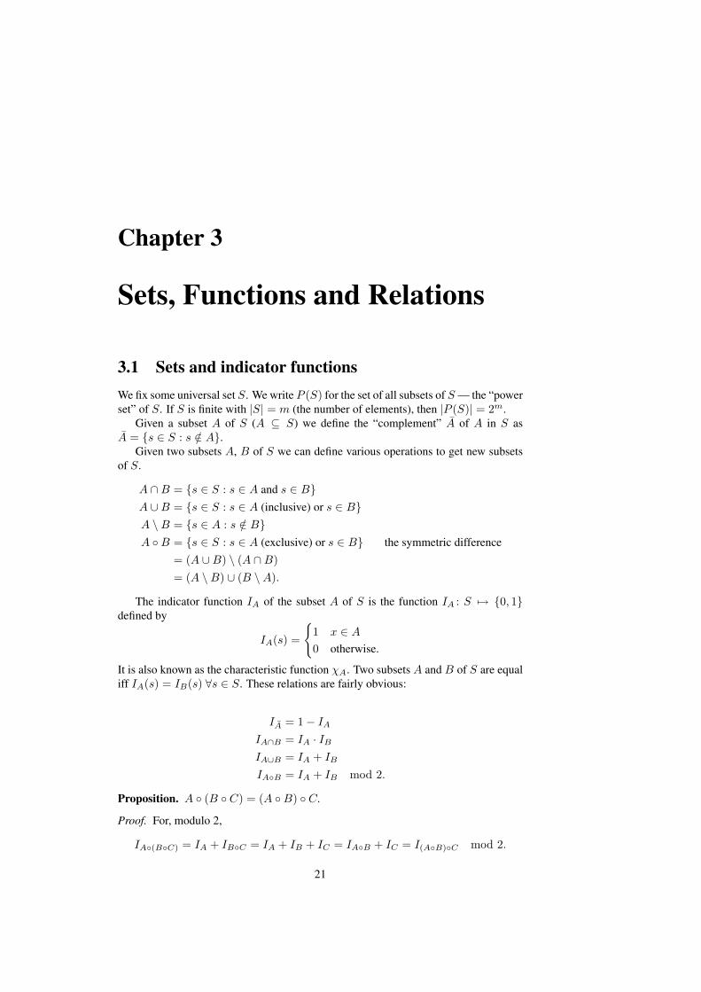
Sets, Functions and Relations

3.1 Sets and indicator functionsWe fix some universal set S. We write P (S) for the set of all subsets of S — the “powerset” of S. If S is finite with |S| = m (the number of elements), then |P (S)| = 2m.

Given a subset A of S (A ⊆ S) we define the “complement” A of A in S asA = {s ∈ S : s /∈ A}.

Given two subsets A, B of S we can define various operations to get new subsetsof S.

A ∩B = {s ∈ S : s ∈ A and s ∈ B}A ∪B = {s ∈ S : s ∈ A (inclusive) or s ∈ B}A \B = {s ∈ A : s /∈ B}A ◦B = {s ∈ S : s ∈ A (exclusive) or s ∈ B} the symmetric difference

= (A ∪B) \ (A ∩B)= (A \B) ∪ (B \A).

The indicator function IA of the subset A of S is the function IA : S 7→ {0, 1}defined by

IA(s) =

{1 x ∈ A

0 otherwise.

It is also known as the characteristic function χA. Two subsets A and B of S are equaliff IA(s) = IB(s) ∀s ∈ S. These relations are fairly obvious:

IA = 1− IA

IA∩B = IA · IB

IA∪B = IA + IB

IA◦B = IA + IB mod 2.

Proposition. A ◦ (B ◦ C) = (A ◦B) ◦ C.

Proof. For, modulo 2,

IA◦(B◦C) = IA + IB◦C = IA + IB + IC = IA◦B + IC = I(A◦B)◦C mod 2.

21

22 CHAPTER 3. SETS, FUNCTIONS AND RELATIONS

Thus P (S) is a group under ◦. Checking the group axioms we get:

• Given A,B ∈ P (S), A ◦B ∈ P (S) — closure,

• A ◦ (B ◦ C) = (A ◦B) ◦ C — associativity,

• A ◦ ∅ = A for all A ∈ P (S) — identity,

• A ◦A = ∅ for all A ∈ P (S) — inverse.

We note that A ◦B = B ◦A so that this group is abelian.

3.1.1 De Morgan’s LawsProposition. 1. A ∩B = A ∪ B

2. A ∪B = A ∩ B

Proof.

IA∩B = 1− IA∩B = 1− IAIB

= (1− IA) + (1− IB)− (1− IA)(1− IB)= IA + IB − IA∩B

= IA∪B .

We prove 2 by using 1 on A and B.

A more general version of this is: Suppose A1, . . . , An ⊆ S. Then

1.⋂n

i=1 Ai =⋃n

i=1 Ai

2.⋃n

i=1 Ai =⋂n

i=1 Ai.

These can be proved by induction on n.

3.1.2 Inclusion-Exclusion PrincipleNote that |A| =

∑s∈S IA(s).

Theorem 3.1 (Principle of Inclusion-Exclusion). Given A1, . . . , An ⊆ S then

|A1 ∪ · · · ∪An| =∑

∅6=J⊆{1,...,n}

(−1)|J|−1 |AJ | , where AJ =⋂i∈J

Ai.

Proof. We consider A1 ∪ · · · ∪An and note that

IA1∪···∪An= IA1∩···∩An

= IA1IA2

. . . IAn

= (1− IA1)(1− IA2) . . . (1− IAn)

=∑

J⊆{1,...,n}

(−1)|J|IAJ,

3.1. SETS AND INDICATOR FUNCTIONS 23

Summing over s ∈ S we obtain the result∣∣A1 ∪ · · · ∪An

∣∣ = ∑J⊆{1,...,n}

(−1)|J| |AJ | ,

which is equivalent to the required result.

Just for the sake of it, we’ll prove it again!

Proof. For each s ∈ S we calculate the contribution. If s ∈ S but s is in no Ai thenthere is a contribution 1 to the left. The only contribution to the right is +1 when J = ∅.If s ∈ S and K = {i ∈ {1, . . . , n} : s ∈ Ai} is non-empty then the contribution to theright is

∑I⊆K(−1)|I| =

∑ki=0

(ki

)(−1)i = 0, the same as on the left.

Example (Euler’s Phi Function).

φ(m) = m∏

p primep|m

(1− 1

p

).

Solution. Let m =∏n

i=1 paii , where the pi are distinct primes and ai ∈ N. Let Ai be

the set of integers less than m which are divisible by pi. Hence φ(m) =∣∣⋂n

i=1 Ai

∣∣.Now |Ai| = m

pi, in fact for J ⊆ {1, . . . ,m} we have |AJ | = mQ

i∈J pi. Thus

φ(m) = m− m

p1− m

p2− · · · − m

pn

+m

p1p2+

m

p1p3+ · · ·+ m

p2p3+ · · ·+ m

pn−1pn

...

+ (−1)n m

p1p2 . . . pn

= m∏

p primep|m

(1− 1

p

)as required.

Example (Derangements). Suppose we have n psychologists at a meeting. Leavingthe meeting they pick up their overcoats at random. In how many ways can this bedone so that none of them has his own overcoat. This number is Dn, the number ofderangements of n objects.

Solution. Let Ai be the number of ways in which psychologist i collects his own coat.Then Dn =

∣∣A1 ∩ · · · ∩ An

∣∣. If J ⊆ {1, . . . , n} with |J | = k then |AJ | = (n − k)!.Thus ∣∣A1 ∩ · · · ∩ An

∣∣ = n!−(

n

1

)(n− 1)! +

(n

2

)(n− 2)!− . . .

= n!n∑

k=0

(−1)k

k!.

Thus Dn is the nearest integer to n! e−1, since Dn

n! → e−1 as n →∞.


3.2 FunctionsLet A,B be sets. A function (or mapping, or map) f : A 7→ B is a way to associatea unique image f(a) ∈ B with each a ∈ A. If A and B are finite with |A| = m and|B| = n then the set of all functions from A to B is finite with nm elements.

Definition. The function f : A 7→ B is injective (or one-to-one) if f(a1) = f(a2)implies that a1 = a2 for all a1, a2 ∈ A.

The number of injective functions from an m-set to an n-set is nm.

Definition. The function f : A 7→ B is surjective (or onto) if each b ∈ B has at leastone preimage a ∈ A.

The number of surjective functions from an m-set to an n-set is n!S(m,n).

Definition. The function f : A 7→ B is bijective if it is both injective and surjective.

If A and B are finite then f : A 7→ B can only be bijective if |A| = |B|. If|A| = |B| < ∞ then any injection is a bijection; similarly any surjection is a bijection.There are n! bijections between two n-sets.

If A and B are infinite then there exist injections which are not bijections and viceversa. For instance if A = B = N, define

f(n) =

{1 n = 1n− 1 otherwise

and g(n) = n + 1.

Then f is surjective but not injective and g is injective but not surjective.

Proposition.

n!S(m,n) =n∑

k=0

(−1)k

(n

k

)(n− k)m

Proof. This is another application of the Inclusion-Exclusion principle. Consider theset of functions from A to B with |A| = m and |B| = n. For any i ∈ B, define Xi tobe the set of functions avoiding i.

So the set of surjections is X1∩· · ·∩Xn. Thus the number of surjections from A toB is

∣∣X1 ∩ · · · ∩ Xn

∣∣. By the inclusion-exclusion principle this is∑

J⊆B(−1)|J| |XJ |.If |J | = k then |XJ | = (n− k)m. The result follows.

Mappings can be “composed”. Given f : A 7→ B and g : B 7→ C we can definegf : A 7→ C by gf(a) = g(f(a)). If f and g are injective then so is gf , similarly forsurjectivity. If we also have h : C 7→ D, then associativity of composition is easilyverified : (hg)f ≡ h(gf).

3.3 PermutationsA permutation of A is a bijection f : A 7→ A. One notation is

f =(

1 2 3 4 5 6 7 81 3 4 2 8 7 6 5

).

The set of permutations of A is a group under composition, the symmetric groupsym A. If |A| = n then sym A is also denoted Sn and |sym A| = n!. Sn is not abelian— you can come up with a counterexample yourself. We can also think of permutationsas directed graphs, in which case the following becomes clear.

3.3. PERMUTATIONS 25

Proposition. Any permutation is the product of disjoint cycles.

We have a new notation for permutations, cycle notation.1 For our function fabove, we write

f = (1)(2 3 4)(5 8)(6 7) = (2 3 4)(5 8)(6 7).

3.3.1 Stirling numbers of the first kindDefinition. s(n, k) is the number of permutations of {1, . . . , n} with precisely k cycles(including fixed points).

For instance s(n, n) = 1, s(n, n − 1) =(n2

), s(n, 1) = (n − 1)!, s(n, 0) =

s(0, k) = 0 for all k, n ∈ N but s(0, 0) = 1.

Lemma 3.1.s(n, k) = s(n− 1, k − 1) + (n− 1)s(n− 1, k)

Proof. Either the point n is in a cycle on its own (s(n−1, k−1) such) or it is not. In thiscase, n can be inserted into any of n− 1 places in any of the s(n− 1, k) permutationsof {1, . . . , n− 1}.

We can use this recurrence to prove this proposition. (Proof left as exercise.)

Proposition.xn =

∑k

s(n, k)xk

3.3.2 Transpositions and shufflesA transposition is a permutation which swaps two points and fixes the rest.

Theorem 3.2. Every permutation is the product of transpositions.

Proof. Since every permutations is the product of cycles we only need to check forcycles. This is easy: (i1 i2 . . . ik) = (i1 i2)(i2 i3) . . . (ik−1 ik).

Theorem 3.3. For a given permutation π, the number of transpositions used to writeπ as their product is either always even or always odd.

We write signπ =

{+1 if always even−1 if always odd

. We say that π is anevenodd permutation.

Let c(π) be the number of cycles in the disjoint cycle representation of π (includingfixed points).

Lemma 3.2. If σ = (a b) is a transposition that c(πσ) = c(π)± 1.

Proof. If a and b are in the same cycle of π then πσ has two cycles, so c(πσ) =c(π)+1. If a and b are in different cycles then they contract them together and c(πσ) =c(π)− 1.

Proof of theorem 3.3. Assume π = σ1 . . . σkι = τ1 . . . τlι. Then c(π) = c(ι) + k ≡c(ι) + l (mod 2). Hence k ≡ l (mod 2) as required.

1See the Algebra and Geometry course for more details.


We note that signπ = (−1)n−c(π), thus sign(π1π2) = signπ1 signπ2 and thussign is a homomorphism from Sn to {±1}.

A k-cycle is an even permutation iff k is odd. A permutation is anevenodd per-

mutation iff the number of even length cycles in the disjoint cycle representation isevenodd .

3.3.3 Order of a permutationIf π is a permutation then the order of π is the least natural number n such that πn = ι.The order of the permutation π is the lcm of the lengths of the cycles in the disjointcycle decomposition of π.

In card shuffling we need to maximise the order of the relevant permutation π. Onecan show (see) that for π of maximal length we can take all the cycles in the disjointcycle representation to have prime power length. For instance with 30 cards we can geta π ∈ S30 with an order of 4620 (cycle type 3 4 5 7 11).

3.3.4 Conjugacy classes in Sn

Two permutations α, β ∈ Sn are conjugate iff ∃π ∈ Sn such that α = πβπ−1.

Theorem 3.4. Two permutations are conjugate iff they have the same cycle type.

This theorem is proved in the Algebra and Geometry course. We note the corollarythat the number of conjugacy classes in Sn equals the number of partitions of n.

3.3.5 Determinants of an n× n matrixIn the Linear Maths course you will prove that if A = (aij) is an n× n matrix then

det A =∑

π∈Sn

signπ

n∏j=1

aj π(j).

3.4 Binary RelationsA binary relation on a set S is a property that any pair of elements of S may or maynot have. More precisely:

Write S×S, the Cartesian square of S for the set of pairs of elements of S, S×S ={(a, b) : a, b ∈ S}. A binary relation R on S is a subset of S × S. We write a R b iff(a, b) ∈ R. We can think of R as a directed graph with an edge from a to b iff a R b.

A relation R is:

• reflexive iff a R a ∀a ∈ S,

• symmetric iff a R b ⇒ b R a ∀a, b ∈ S,

• transitive iff a R b, b R c ⇒ a R c ∀a, b, c ∈ S,

• antisymmetric iff a R b, b R a ⇒ a = b ∀a, b ∈ S.

3.5. POSETS 27

The relation R on S is an equivalence relation if it is reflexive, symmetric andtransitive. These are “nice” properties designed to make R behave something like =.

Definition. If R is a relation on S, then

[a]R = [a] = {b ∈ S : a R b}.

If R is an equivalence then these are the equivalence classes.

Theorem 3.5. If R is an equivalence relation then the equivalence classes form apartition of S.

Proof. If a ∈ S then a ∈ [a], so the classes cover all of S. If [a] ∩ [b] 6= ∅ then∃c ∈ [a] ∩ [b]. Now a R c and b R c ⇒ c R b. Thus a R b and b ∈ [a]. If d ∈ [b]then b R d so a R d and thus [b] ⊆ [a]. We can similarly show that [a] ⊆ [b] and thus[a] = [b].

The converse of this is true: if we have a partition of S we can define an equivalencerelation on S by a R b iff a and b are in the same part.

An application of this is the proof of Lagrange’s Theorem. The idea is to show thatbeing in the same (left/right) coset is an equivalence relation.

Given an equivalence class on S the quotient set is S/R, the set of all equivalenceclasses. For instance if S = R and a R b iff a − b ∈ Z then S/R is (topologically) acircle. If S = R2 and (a1, b1) R (a2, b2) iff a1 − a2 ∈ Z and b1 − b2 ∈ Z the quotientset is a torus.

Returning to a general relation R, for each k ∈ N we define

R(k) = {(a, b) : there is a path of length at k from a to b}.

R(1) = R and R(∞) = t(R), the transitive closure of R. R(∞) is defined as⋃i≥1R(i).

3.5 PosetsR is a (partial) order on S if it is reflexive, anti-symmetric and transitive. The set S isa poset (partially ordered set) if there is an order R on S.

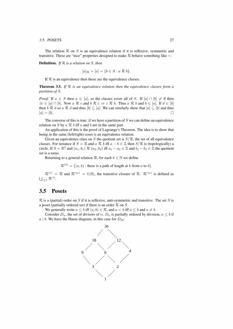
We generally write a ≤ b iff (a, b) ∈ R, and a < b iff a ≤ b and a 6= b.Consider Dn, the set of divisors of n. Dn is partially ordered by division, a ≤ b if

a | b. We have the Hasse diagram, in this case for D36:

36

18 12

9

3

46

2

1


A descending chain is a sequence a1 > a2 > a3 > . . . . An antichain is a subset ofS with no two elements directly comparable, for instance {4, 6, 9} in D36.

Proposition. If S is a poset with no chains of length > n then S can be covered by atmost n antichains.

Proof. Induction on n. Take n > 1 and let M be the set of all maximal elements in S.Now S \M has no chains of length > n− 1 and M is an antichain.

3.5.1 Products of posetsSuppose A and B are posets. Then A×B has various orders; two of them being

• product order: (a1, b1) ≤ (a2, b2) iff a1 ≤ a2 and b1 ≤ b2,

• lexicographic order: (a1, b1) ≤ (a2, b2) if either a1 ≤ a2 or if a1 = a2 thenb1 ≤ b2.

Exercise: check that these are orders.Note that there are no infinite descending chains in N × N under lexicographic

order. Such posets are said to be well ordered. The principle of induction follows fromwell-ordering as discussed earlier.

3.5.2 Eulerian DigraphsA digraph is Eulerian if there is a closed path covering all the edges. A necessarycondition is: the graph is connected and even (each vertex has an equal number of “in”and “out” edges). This is in fact sufficient.

Proposition. The set of such digraphs is well-ordered under containment.

Proof. Assume proposition is false and let G be a minimal counterexample. Let T bea non-trivial closed path in G, for instance the longest closed path. Now T must beeven, so G \ T is even. Hence each connected component of G \ T is Eulerian as Gis minimal. But then G is Eulerian: you can walk along T and include all edges ofconnected components of G \ T when encountered — giving a contradiction. Hencethere are no minimal counterexamples.

3.6 CountabilityDefinition. A set S is countable if either |S| < ∞ or ∃ a bijection f : S 7→ N.

The countable sets can be equivalently thought of as those that can be listed on aline.

Lemma 3.3. Any subset S ⊂ N is countable.

Proof. For: map the smallest element of S to 1, the next smallest to 2 and so on.

Lemma 3.4. A set S is countable iff ∃ an injection f : S 7→ N.

Proof. This is clear for finite S. Hence assume S is infinite. If f : S 7→ N is aninjection then f(S) is an infinite subset of N. Hence ∃ a bijection g : f(S) 7→ N. Thusgf : S 7→ N is a bijection.

3.6. COUNTABILITY 29

An obvious result is that if S′ is countable and ∃ an injection f : S 7→ S′ then S iscountable.

Proposition. Z is countable.

Proof. Consider f : Z 7→ N,

f : x 7→

{2x + 1 if x ≥ 0−2x if x < 0.

This is clearly a bijection.

Proposition. Nk is countable for k ∈ N.

Proof. The map (i1, . . . , ik) 7→ 2i13i2 . . . pik

k (pj is the jth prime) is an injection byuniqueness of prime factorisation.

Lemma 3.5. If A1, . . . , Ak are countable with k ∈ N, then so is A1 × · · · ×Ak.

Proof. Since Ai is countable there exists an injection fi : Ai 7→ N. Hence the functiong : A1, . . . , Ak 7→ Nk defined by g(a1, . . . , ak) = (f1(a1), . . . , fk(ak)) is an injection.

Proposition. Q is countable.

Proof. Define f : Q 7→ N by

f :a

b7→ 2|a|3b51+sign a,

where (a, b) = 1 and b > 0.

Theorem 3.6. A countable union of countable sets is countable. That is, if I is acountable indexing set and Ai is countable ∀i ∈ I then

⋃i∈I Ai is countable.

Proof. Identify first I with the subset f(I) ⊆ N. Define F : A 7→ N by a 7→ 2n3m

where n is the smallest index i with a ∈ Ai, and m = fn(a). This is well-defined andinjective (stop to think about it for a bit).

Theorem 3.7. The set of all algebraic numbers is countable.

Proof. Let Pn be the set of all polynomials of degree at most n with integral coeffi-cients. Then the map cnxn + · · ·+ c1x+ c0 7→ (cn, . . . , c1, c0) is an injection from Pn

to Zn+1. Hence each Pn is countable. It follows that the set of all polynomials withintegral coefficients is countable. Each polynomial has finitely many roots, so the setof algebraic numbers is countable.

Theorem 3.8 (Cantor’s diagonal argument). R is uncountable.

Proof. Assume R is countable, then the elements can be listed as

r1 = n1.d11d12d13 . . .

r2 = n2.d21d22d13 . . .

r3 = n3.d31d32d33 . . .

(in decimal notation). Now define the real r = 0.d1d2d3 . . . by di = 0 if dii 6= 0 anddi = 1 if dii = 0. This is real, but it differs from ri in the ith decimal place. So the listis incomplete and the reals are uncountable.


Exercise: use a similiar proof to show that P (N) is uncountable.

Theorem 3.9. The set of all transcendental numbers is uncountable. (And therefore atleast non-empty!)

Proof. Let A be the set of algebraic numbers and T the set of transcendentals. ThenR = A ∪ T , so if T was countable then so would R be. Thus T is uncountable.

3.7 Bigger setsThe material from now on is starred.

Two sets S and T have the same cardinality (|S| = |T |) if there is a bijectionbetween S and T . One can show (the Schroder-Bernstein theorem) that if there is aninjection from S to T and an injection from T to S then there is a bijection between Sand T .

For any set S, there is an injection from S to P (S), simply x 7→ {x}. Howeverthere is never a surjection S 7→ P (S), so |S| < |P (S)|, and so

|N| < |P (N)| < |P (P (N))| < . . .

for some sensible meaning of <.

Theorem 3.10. There is no surjection S 7→ P (S).

Proof. Let f : S 7→ P (S) be a surjection and consider X ∈ P (S) defined by {x ∈S : x /∈ f(x)}. Now ∃x′ ∈ S such that f(x′) = X . If x′ ∈ X then x′ /∈ f(x′) butf(x′) = X — a contradiction. But if x′ /∈ X then x′ /∈ f(x′) and x′ ∈ X — giving acontradiction either way.

If there is aninjectionsurjection f : A 7→ B then there exists a

surjectioninjection g : B 7→ A.

Moreover we can ensure thatg ◦ f = ιAf ◦ g = ιB

References

◦ Hardy & Wright, An Introduction to the Theory of Numbers, Fifth ed., OUP, 1988.

This book is relevant to quite a bit of the course, and I quite enjoyed (parts of!) it.

◦ H. Davenport, The Higher Arithmetic, Sixth ed., CUP, 1992.

A very good book for this course. It’s also worth a read just for interest’s sake.

I’ve also heard good things about Biggs’ book, but haven’t read it.

31

discrete mathematics - the archimedeans induction and counting 11 2.1 the pigeonhole principle ......

Documents