discrete mathematics lecture notesmatematika.fri.uni-lj.si/dm/discrete_mathematics.pdf · the...

DISCRETE MATHEMATICS

lecture notes

Gasper Fijavz

Faculty of Computer and Information Science

Ljubljana, November 2014

CIP - Kataložni zapis o publikaciji Narodna in univerzitetna knjižnica, Ljubljana 51(075.8)(0.034.2) FIJAVŽ, Gašper Discrete mathematics [Elektronski vir] : lecture notes / Gašper Fijavž. - El. knjiga. - Ljubljana : Fakulteta za računalništvo in informatiko, 2014 Način dostopa (URL): http://matematika.fri.uni-lj.si/discrete_mathematics.pdf ISBN 978-961-6209-84-7 (pdf) 277297152

Contents

Uvod 4

Introduction 4

1 Graph Searching 5

2 Paths, flows, and connectivity 14

3 Constructing 2-connected graphs 25

4 Planar graphs 37

5 Discharging technique 46

6 List coloring of planar graphs 56

7 Chordal graphs 62

8 Tree decomposition 70

9 Tree decomposition lower bounds 79

10 Matchings 83

3 DM, lecture notes

Uvod

Predmet Diskretna matematika studenta popelje na podrocje zahtevnejsih grafovskihalgoritmov, ki jih obravnavamo delno z matematicnega in delno z racunalniskegavidika.

Zdi se, da so algoritmicni problemi na grafih ali zelo enostavni, taksne algoritmesrecamo pri tecaju iz algoritmov in podatkovnih struktur, ali pa NP-tezki. Pridiskretni matematiki bomo poskusili najti srednjo pot, vecinoma se bomo drzali vbazenu polinomsko resljivih problemov, ki presegajo osnovno algoritmicno solo.

Za uspesen studij taksnih problemov pa bo potrebno nekaj novih matematicnihznanj.

Predmet Diskretna matematika izvajamo v angleskem jeziku, pricujoci zapiski pre-davanj pa so dostopni tudi na spletnem naslovu

matematika.fri.uni-lj.si/discrete_mathematics.pdf

Introduction

The Discrete mathematics course tackles a selection of graph algorithms, which arestudied from both the mathematical and computational point of view.

We often have the impression that graph algorithmic problems are either very basic,and as such taught in an introductory algorithms course, or NP-hard. This coursetries to steer in between. We shall mostly study problems that are computationallyeasy—solvable in polynomial time, yet difficult enough to surpass the collection ofelementary algorithms.

We shall need quite a lot of discrete mathematical background to successfully dealwith these types of problems, and the details are provided herein.

These lecture notes are available at


4 DM, lecture notes



1 Graph Searching

1.1 Definitions

Let G be a graph. We say that vertex u is reachable from a vertex v, u v, if thereexists a path Puv (equivalently a walk) starting at u and ending at v. In case G isa directed graph also the path Puv is supposed to be a directed one.

Reachability is trivially — using paths of length 0 — a reflexive relation on the setV (G). If G is undirected, then reachability is also symmetric and transitive.

Let G temporarily denote an undirected graph. Reachability, being an equivalencerelation, partitions the set V (G) into equivalence sets V1, V2, V3, . . . , Vk, and theinduced graphs C1 = G[V1], C2 = G[V2], C3 = G[V3], . . . , Ck = G[Vk] are calledconnected components of G. In case G has a single connected component we call Ga connected graph.

A component Ci of G is a maximal connected induced subgraph of G.

The story is somewhat different in the case of directed graphs. If−→G is a directed

graph it might happen that a vertex is reachable from another but not vice-versa,u v and v 6 u, the relation not being symmetric. Yet the relation of mutualreachability , u v and v u, is an equivalence relation, and similarly as above,

decomposes the graph−→G into strongly connected components (s.c. components)

−→C 1,−→C 2, . . . ,

−→C `. As above, a strongly connected component is a maximal strongly

connected component of−→G .

If−→G is a directed graph, then its underlying graph G is obtained by removing

orientations of edges of−→G , keeping the same vertex set, and suppressing possible

parallel edges obtained by deleting orientations of a pair of counter oriented edges.

Clearly, if−→G is strongly connected, then G is connected, but the reverse may not

hold. We call−→G weakly connected if its underlying counterpart G is connected. Note

that weak connectivity of−→G does not imply that for arbitrary vertices u, v ∈ V (

−→G)

at least one is reachable from the other.

In order to keep our results tidier we shall also say that a connected undirectedgraph G is strongly connected as well.

Let us now define distance between vertices in G: the distance from x to y, dist(x, y),

is the length of a shortest x→ y-path in−→G . Note that in a directed graph

−→G

the distances dist(x, y) and dist(y, x) may be different, yet in an undirected graphdistance is symmetric.

We call−→G a directed acyclic graph or dag (for short) if

−→G has no directed cycles

— a pair of counter oriented edges is considered a cycle of length 2. Observe that

its underlying graph G may contain cycles. A topological ordering of vertices of−→G

is a linear ordering v1, v2, v3, . . . , vn (numbering of vertices), so that if vivj ∈ E(−→G)

then i < j. In other words, with respect to the topological ordering, every edge ispointing to the right.

5 DM, lecture notes

If−→G is not a dag then its vertices cannot be topologically ordered. Irrespective

of the numbering of vertices, traversing a directed cycle necessarily makes at least

one step to the left. Does the reverse implication also hold? If−→G is a dag, do its

vertices admit a topological ordering? The easiest argument is inductive: if−→G is

a dag, then there exists a vertex v satisfying outdeg(v) = 0 (otherwise every walk

can be extended by an additional step,−→G admits walks with repeated vertices, and

the shortest walk with repeated vertices is a directed cycle). Now v can be put as

the last vertex in the topological ordering, and vertices of−→G − v can be ordered

recursively.

1.2 Graph searching, general schema

We can picture graph searching like a disease infecting vertices which is spreadingalong (directed) edges. Initially, vertices are healthy, and in the beginning a vertex,often called the root , gets infected. The process stabilizes when no new infectionsare possible, and it might happen that not all vertices are infected. In this case wemay restart by infecting another vertex.

We shall rather use colors for indicating whether a vertex has been visited with asearch algorithm. A vertex is white if it has not been discovered with a searchingprocedure, and infection turns the vertex black (like plague or black death, right).Upon discovery a vertex is put in a data structure D. Initially all vertices are coloredwhite, D is empty, and an auxiliary structure search forest T is trivial.

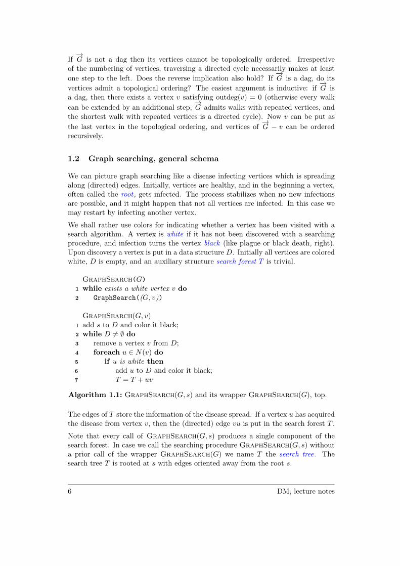
GraphSearch(G)1 while exists a white vertex v do2 GraphSearch((G, v))

GraphSearch(G, v)1 add s to D and color it black;2 while D 6= ∅ do3 remove a vertex v from D;4 foreach u ∈ N(v) do5 if u is white then6 add u to D and color it black;7 T = T + uv

Algorithm 1.1: GraphSearch(G, s) and its wrapper GraphSearch(G), top.

The edges of T store the information of the disease spread. If a vertex u has acquiredthe disease from vertex v, then the (directed) edge vu is put in the search forest T .

Note that every call of GraphSearch(G, s) produces a single component of thesearch forest. In case we call the searching procedure GraphSearch(G, s) withouta prior call of the wrapper GraphSearch(G) we name T the search tree. Thesearch tree T is rooted at s with edges oriented away from the root s.

6 DM, lecture notes

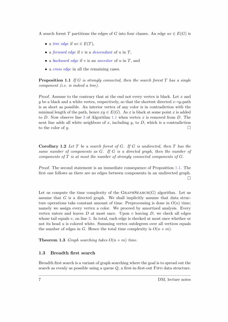
A search forest T partitions the edges of G into four classes. An edge uv ∈ E(G) is

• a tree edge if uv ∈ E(T ),

• a forward edge if v is a descendant of u in T ,

• a backward edge if v is an ancestor of u in T , and

• a cross edge in all the remaining cases.

Proposition 1.1 If G is strongly connected, then the search forest T has a singlecomponent (i.e. is indeed a tree).

Proof. Assume to the contrary that at the end not every vertex is black. Let x andy be a black and a white vertex, respectively, so that the shortest directed x→y-pathis as short as possible. An interior vertex of any color is in contradiction with theminimal length of the path, hence xy ∈ E(G). As x is black at some point x is addedto D. Now observe line 3 of Algorithm 1.1 when vertex x is removed from D. Thenext line adds all white neighbors of x, including y, to D, which is a contradictionto the color of y. �

Corollary 1.2 Let T be a search forest of G. If G is undirected, then T has thesame number of components as G. If G is a directed graph, then the number ofcomponents of T is at most the number of strongly connected components of G.

Proof. The second statement is an immediate consequence of Proposition 1.1. Thefirst one follows as there are no edges between components in an undirected graph.

�

Let us compute the time complexity of the GraphSearch(G) algorithm. Let usassume that G is a directed graph. We shall implicitly assume that data struc-ture operations take constant amount of time. Preprocessing is done in O(n) time;namely we assign every vertex a color. We proceed by amortized analysis. Everyvertex enters and leaves D at most once. Upon v leaving D, we check all edgeswhose tail equals v, on line 3. In total, each edge is checked at most once whether ornot its head u is colored white. Summing vertex outdegrees over all vertices equalsthe number of edges in G. Hence the total time complexity is O(n+m).

Theorem 1.3 Graph searching takes O(n+m) time.

1.3 Breadth first search

Breadth first search is a variant of graph searching where the goal is to spread out thesearch as evenly as possible using a queue Q, a first-in-first-out Fifo data structure.

7 DM, lecture notes

BFS(G)1 while exists a white vertex v do2 BFS (G, v)

BFS(G, s)1 EnQueue (s,Q);2 while Q 6= ∅ do3 v=DeQueue (Q);4 foreach u ∈ N(v) do5 if u is white then6 EnQueue (u,Q) and color u black;7 add edge vu to search forest T

Algorithm 1.2: BFS(G, s) and its wrapper BFS(G), top.

Breadth first search is typically the preferred choice for computing connected com-ponents of an undirected graph.

Let us begin by observing that at every time of the run of BFS(G, s), the verticesin Q are ordered by their distances from s, and even more:

Proposition 1.4 Let x1, x2, x3, . . . , xk is the sequence of vertices in Q at an arbi-trary instant of the run of BFS(G, s). Then

(a) dist(s, x1) ≤ dist(s, x2) ≤ dist(s, x3) ≤ . . . ≤ dist(s, xk), and

(b) dist(s, xk) ≤ dist(s, x1) + 1.

Proof. We omit this proof �

We can nonetheless exploit the spread of searching in BFS(G, s) to compute dis-tances from a fixed vertex s to the other vertices in G. Next, an s→x path in T isalso a shortest s→x path in G. Let x be an ancestor of y in T . Then let distT (x, y)denote the length of the x→y-path in T . Obviously distT (x, y) ≥ dist(x, y). A littleless obvious is the converse:

Proposition 1.5 Let x be an ancestor of y in T . Then distT (x, y) = dist(x, y).

Proof. It is enough to prove the result for the case x = s is the root of T . Lets = x0, x1, x2, . . . , xk−1, xk = y be the sequence of vertices along the shortestand only s→y-path in T , so that k = distT (s, y) > dist(s, y). This implies thatdist(s, y) = dist(s, xk−1) = k − 1. Let y′ be a vertex adjacent to y on some shortests→y-path, in particular y′ 6= xk−1. By Proposition 1.4 y′ has entered Q before xk−1.As y′y is not a tree edge, y was already colored black by the time y′ has left Q.This is impossible, as xk−1, the predecessor of y, did not leave Q before y′, again by

8 DM, lecture notes

Proposition 1.4. �

Now Proposition 1.5 has an immediate consequence.

Theorem 1.6 If T is a BFS-tree of G with root s, then T contains shortest pathfrom s to every vertex v of G which is reachable from s, and both distances from sand instances of shortest s→v paths.

Proof. Distances from s can be computed by a simple modification of BFS(G, s).Let us first set d(v) = ∞ for every v ∈ V (G) \ {s}, and set d(s) = 0, and runBFS(G, s) with an additional line

8 d(u) = d(v) + 1

�

1.4 Depth first search

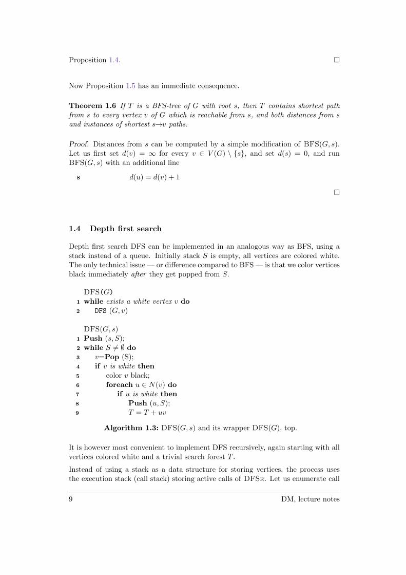
Depth first search DFS can be implemented in an analogous way as BFS, using astack instead of a queue. Initially stack S is empty, all vertices are colored white.The only technical issue — or difference compared to BFS — is that we color verticesblack immediately after they get popped from S.

DFS(G)1 while exists a white vertex v do2 DFS (G, v)

DFS(G, s)1 Push (s, S);2 while S 6= ∅ do3 v=Pop (S);4 if v is white then5 color v black;6 foreach u ∈ N(v) do7 if u is white then8 Push (u, S);9 T = T + uv

Algorithm 1.3: DFS(G, s) and its wrapper DFS(G), top.

It is however most convenient to implement DFS recursively, again starting with allvertices colored white and a trivial search forest T .

Instead of using a stack as a data structure for storing vertices, the process usesthe execution stack (call stack) storing active calls of DFSr. Let us enumerate call

9 DM, lecture notes

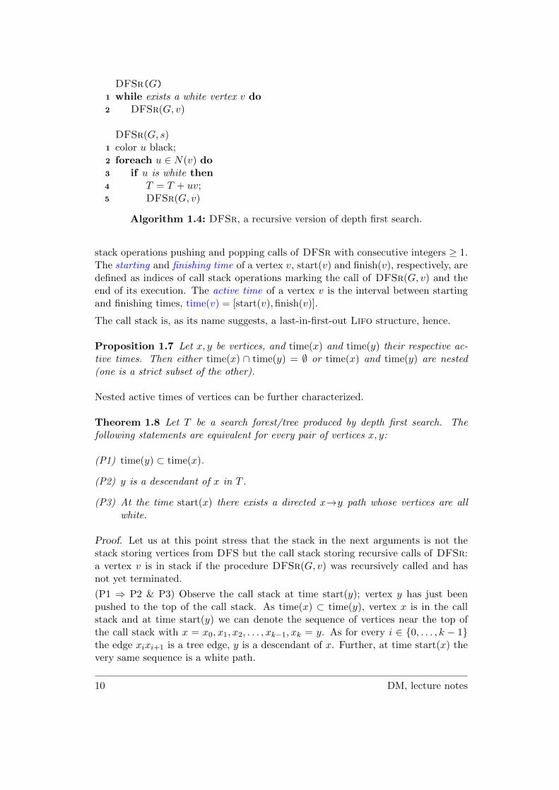
DFSr(G)1 while exists a white vertex v do2 DFSr(G, v)

DFSr(G, s)1 color u black;2 foreach u ∈ N(v) do3 if u is white then4 T = T + uv;5 DFSr(G, v)

Algorithm 1.4: DFSr, a recursive version of depth first search.

stack operations pushing and popping calls of DFSr with consecutive integers ≥ 1.The starting and finishing time of a vertex v, start(v) and finish(v), respectively, aredefined as indices of call stack operations marking the call of DFSr(G, v) and theend of its execution. The active time of a vertex v is the interval between startingand finishing times, time(v) = [start(v),finish(v)].

The call stack is, as its name suggests, a last-in-first-out Lifo structure, hence.

Proposition 1.7 Let x, y be vertices, and time(x) and time(y) their respective ac-tive times. Then either time(x) ∩ time(y) = ∅ or time(x) and time(y) are nested(one is a strict subset of the other).

Nested active times of vertices can be further characterized.

Theorem 1.8 Let T be a search forest/tree produced by depth first search. Thefollowing statements are equivalent for every pair of vertices x, y:

(P1) time(y) ⊂ time(x).

(P2) y is a descendant of x in T .

(P3) At the time start(x) there exists a directed x→y path whose vertices are allwhite.

Proof. Let us at this point stress that the stack in the next arguments is not thestack storing vertices from DFS but the call stack storing recursive calls of DFSr:a vertex v is in stack if the procedure DFSr(G, v) was recursively called and hasnot yet terminated.

(P1 ⇒ P2 & P3) Observe the call stack at time start(y); vertex y has just beenpushed to the top of the call stack. As time(x) ⊂ time(y), vertex x is in the callstack and at time start(y) we can denote the sequence of vertices near the top ofthe call stack with x = x0, x1, x2, . . . , xk−1, xk = y. As for every i ∈ {0, . . . , k − 1}the edge xixi+1 is a tree edge, y is a descendant of x. Further, at time start(x) thevery same sequence is a white path.

10 DM, lecture notes

(P2 ⇒ P1) The call of DFSr(G, x) is not yet finished at the start of the callDFSr(G, y). Hence the inclusion of active times.

(P3 ⇒ P2) Assume that there exists a pair of vertices x, y, a path Px,y definedby x = x0, x1, x2, . . . , xk−1, xk = y which is white at start(x), and let us also as-sume that y is not a descendant of x in T . We may assume that the pair x, y ischosen so that Px,y is as short as possible. This implies that vertices x1, . . . , xk−1are all descendants of x, which in turn implies time(xk−1) ⊆ time(x) (by (P1)applied to x and xk−1 taking into account that k might be 1). As being a descen-dant is a transitive relation we may assume that y is not a descendant of xk−1.Hence time(xk) ∩ time(y) = ∅. Now start(y) > finish(xk−1) contradicts the defini-tion of BFSr, and finish(y) < start(xk−1)(< finish(xk−1) < finish(x)) implies thattime(y) 6⊂ time(x) as y is not a descendant of x nor finish(y) < start(x) as y is whiteat time start(x). This is a contradiction. �

1.5 Applications of DFS: topological sort and strongly connectedcomponents

In this section we will show how to use DFS to topologically sort vertices of a dagand how to compute strongly connected components of a directed graph using tworuns of DFS.

Proposition 1.9−→G admits a topological ordering if and only if

−→G is a directed

acyclic graph.

�

Let us start with a DFS-based computation of a topological ordering. Let L bea list, which is initially empty. TopologicalSort can be defined with a single(albeit not simple) line of pseudocode.

TopologicalSort(−→G)

1 run DFSr(−→G) and at the finish of each DFSr(

−→G, v) prepend vertex v to L

Algorithm 1.5: TopologicalSort

Observe that at the end of the run the list L contains vertices of G sorted accordingto descending finishing time. The following proposition establishes correctness ofAlgorithm 1.5

Proposition 1.10 Let−→G be a dag, and let DFSr compute the finishing times of

its vertices. If xy ∈ E(−→G) then finish(x) > finish(y).

Proof. If xy ∈ E(−→G) then y 6 x, as

−→G is a dag. Hence, at no time there exists a

white y→x-path, and by Theorem 1.8 x is not a descendant of y, or equivalently


time(x) 6⊂ time(y). Now start(y) > finish(x) contradicts the run of DFSr, henceon one hand start(y) < finish(x). Together with time(x) 6⊂ time(y) this impliesfinish(y) < finish(x). �

Let−→G be a directed graph. A component graph of

−→G , also called condensation of−→

G , is a directed graph−→Gcond defined in the following way: vertices of

−→Gcond are

strongly connected components C1, C2, . . . , C` of−→G , and CiCj ∈ E(

−→Gcond) if there

exists an edge xixj ∈ E(−→G), so that xi ∈ V (Ci) and xj ∈ V (Cj).

Let−→G be a directed graph. Its reverse graph

←−G is obtained by reversing orientations

of all edges of−→G . Observe that strongly connected components of both

−→G and

←−G

are the same. Namely, if a pair of vertices x, y are mutually reachable, then theyare also mutually reachable if we reverse all edge orientations.

We can compute strongly connected components in two consecutive runs of depthfirst search. Let L be a list, which is initially empty.

StronglyConnectedComponents(−→G)

1 run DFSr(−→G) and at the finish of each DFSr(

−→G, v) prepend vertex v to L

reverse edges to compute←−G ;

2 run DFSr(←−G) in the order as the vertices appear in L and compute the

search forest T ;

3 vertex-sets of components of T induce strongly connected components of−→G

Algorithm 1.6: StronglyConnecteComponents

Before proving correctness of the above algorithm we need to establish some technicalresults.

Proposition 1.11 Let C1 and C2 be distinct strongly connected components of−→G .

If there exists an edge x1x2 ∈ E(−→G), then no vertex of C1 is reachable from a vertex

of C2.

Proof. Assume that y2 y1 for some y1 ∈ V (C1) and y2 ∈ V (C2). As x2 y2 andy1 x1, vertices x1 and x2 are mutually reachable. This contradicts the fact thatthey lie in different strongly connected component. �

An immediate consequence of Proposition 1.11 is the next corrolary which we statewithout its proof.

Corollary 1.12 Every component graph−→Gcond is a dag.

Let us first extend starting and finishing times to subgraphs of−→G . If

−→H ⊆

−→G , then

its starting time start(−→H ) is defined as start(

−→H ) = min{start(v) | v ∈ V (

−→H )}.


Similarly we define its finishing time finish(−→H ) as finish(

−→H ) = max{finish(v) | v ∈

V (−→H )}.

We shall first compare finishing times of adjacent strongly connected components.

Proposition 1.13 Let C1 and C2 be distinct strongly connected components of−→G .

If there exists an edge x1x2 ∈ E(−→G) with x1 ∈ V (C1) and x2 ∈ V (C2), then

finish(C2) < finish(C1).

Proof. Let x ∈ V (C1)∪V (C2) be the vertex satisfying start(x) = min{start(C1), start(C2)}.If x ∈ V (C1) then for every vertex y ∈ V (C2) there exists a directed x→y-path whosevertices are at time start(x) all white. Hence every vertex of C2 is a descendant ofx, and finish(C2) < finish(y) ≤ finish(C1).

Next assume that x ∈ V (C2). As above, for every vertex y ∈ V (C2) there exists adirected x→y-path whose vertices are at time start(x) all white. Hence, by nestingof active times we have finish(C2) = finish(x). Let x1 be an arbitrary vertex of C1.By the choice of x we have start(x) < start(x1), and since x1 is not a descendant ofx (by Theorem 1.8 and Proposition 1.11, as x 6 x1) we have finish(x) < finish(x1),and the proof is finished. �

We are now in the position to prove correctness of Algorithm 1.6.

Theorem 1.14 StronglyConnectedComponents(−→G) correctly computes strongly

connected components of−→G .

Proof. Let C1, C2, C3, . . . , C` be the strongly connected components sorted by de-creasing finishing time implicitly computed on line 1 of Algorithm 1.6. Proposi-

tion 1.13 states that they are indeed topologically ordered. As the routine DFSr(−→G, x)

cannot visit a proper nonempty subset of vertices of some strongly connected com-ponent we shall inductively assume that the call StronglyConnectedCompo-

nents(−→G) has at some point correctly identified strongly connected components

C1, . . . , Ck−1, and did not visit vertices outside these components. The inductionbasis is trivial.

As an inductive step we only need to see that the search tree Tk produced by the

call DFSr(←−G, vk) (where vk is an arbitrary vertex of Ck) satisfies V (Tk) = V (Ck).

Clearly V (Ck) ⊆ V (Tk), as all vertices of Ck are reachable from vk and are also

white at time start(vk). Let xy ∈←−G so that x ∈ V (Ck) and y ∈ V (Cj) for some

j 6= k. By Proposition 1.13 we have finish(Ck) < finish(Cj) or equivalently j < k.This implies that y is black. Hence at time start(vk) every white path starting atvk ends in a vertex of Ck. Theorem 1.8 implies that V (Tk) ⊆ V (Ck), which finishesthe proof. �


2 Paths, flows, and connectivity

Imagine that we want to transfer information originating in a vertex u to a distantvertex v. As information can only be passed along edges, a single u→ u′-pathsuffices for the task. On the other hand there might be an attacker trying to stopthe information transfer by either deleting edges or deleting vertices. If we canfind several independent ways to transfer information then an attacker possible ofcompromising only a few structures in our graph cannot stop the information flow.

We will try to look at the problem from both parties’ ways. On one hand we wantto find as many independent u→u′-paths in G, on the other we shall look for astructure as small as possible, whose removal inhibits the spread of information.

2.1 Menger theorems

Let G be a (directed) graph, and let u and u′ be different vertices of G. We saythat u→u′ paths P1 and P2 are edge disjoint if E(P1) ∩ E(P2) = ∅, and P1 and P2

are internally disjoint if V (P1)∩V (P2) = {u, u′}. In other words, internally disjointu→v-paths do not share vertices nor edges, apart from their endvertices.

Assume that we want to find a collection P of edge-disjoint u→u′-paths whosecardinality is as large as possible. Is there an easy upper bound on |P|? Clearly|P| ≤ outdeg(u) and also |P| ≤ indeg(u′). More generally, let us partition verticesof G into two parts, one containing u and the other containing u′. The number ofedges from the first part to the second is also an upper bound for the number ofpaths in P.

To be precise given vertices u and u′, an u, u′-cut is an edge set E(U,U ′) = {xy ∈E(G) | x ∈ U and y ∈ U ′}, for which U,U ′ is a partition of V (G) (U ∪U ′ = V (G),U ∩ U ′ = ∅) so that u ∈ U and u′ ∈ U ′.

Theorem 2.1 (Menger, 1.0) Let G be a (directed) graph, u and u′ distinct ver-tices. The maximal number of edge disjoint u→u′-paths is equal to the size of thesmallest u, u′-cut.

We shall postpone the proof of Theorem 2.1 until later. But let us at this pointstress the duality aspect: for every collection of edge-disjoint u→u′-paths P andevery u, u′-cut C we have |P| ≤ |C|. Now an equality implies optimality of both, notonly that P is as large as possible, but also that C is as small as possible.

But the story goes on. Let G be an undirected graph and assume that S ⊆ V (G−u − u′) is a set of vertices so that vertices u and u′ lie in different components ofG− S. This implies that every u− u′-path of G uses a vertex of S. We call such avertex set S a u, v-separator . As two internally disjoint u − u′-paths cannot sharea vertex from S, |S| is clearly an upper bound on the number of internally disjointu− u′-paths. Menger has proven yet another version of the theorem (and its proofwe shall again postpone until later):


Theorem 2.2 (Menger, 2.0) Let G be an undirected graph and u and u′ distinctnonadjacent vertices. The maximal number of internally disjoint u−u′-paths is equalto the order of the smallest u, u′-separator.

As above, the importance lies in the duality. Clearly the number of internallydisjoint u − u′-paths cannot exceed the size of any u, u′-separator. The essence ofTheorem 2.2 lies in the equality in the extremal cases.

Is nonadjacency really necessary? Well, if u and u′ were adjacent, they cannot beseparated by deleting vertices only.

But what if one would like to have truly disjoint paths? Let A, B be vertex sets andlet us look for collections of disjoint A−B-paths in an undirected graph G. Clearlyboth |A| and |B| are upper bounds on the cardinality of such a collection.

Note that in case A and B are not disjoint, the singleton paths from A ∩ B forma collection of A − B-paths, and for the rest we can look for A \ B − B \ A-pathsbetween disjoint vertex sets in G− (A ∩B).

Menger has an appropriate result in this case as well, and we apologize once morefor postponing the proof.

Theorem 2.3 (Menger, 3.0) Let A,B be vertex sets of an undirected graph G.The maximal number of disjoint A−B-paths is equal to the order of smallest vertexset S, so that G− S contains no A−B-paths.

Note that in Theorem 2.3 we allow S to contain vertices from A ∪B.

2.2 Flows

The above Menger theorems (there are more to come), though dealing with differenttypes of graph structure, appear to be similar enough so a common approach shouldtake care of all their proofs. This is indeed the case, but we will have to make adetour into the class of weighted graphs.

Again let us use the transfer of information example. Two links between nodes ina network may have different bandwidths. Two pipes in a water supply networkmay have different diameters. The amount of information or water flowing on aconnection may differ from one place to another, but in principle can be anythingbetween zero and the connection’s capacity.

Hence, weighted graphs. A weighted graph Gw , is a directed graph together with amapping

w : E(−→G)→ R+.

The weight of a directed edge uv is its w-value w(uv).

We say that weights are symmetric if w(uv) = w(vu) for every directed edge. In thiscase we shall talk about weighted undirected graphs. Similarly, an unweighted graph


(directed or undirected) may be modeled with 0/1 weights. We shall call weights ofedges also capacities, and regard an edge uv with w(uv) = 0 as a nonedge in Gw.

Let Gw be a weighted graph and s, t vertices, called source and sink respectively.An s-t-flow f is a mapping

f : E(Gw)→ R+

satisfying

(F1) 0 ≤ f(uv) ≤ w(uv) and

(F2)∑

x∈N(v) f(vx)−∑

v∈N(y) f(yv) = 0 for every vertex v 6= s, t.

Condition (F1) states that edge-flow is nonnegative and bounded from above byedge-weight, and conditions (F2) are also called Kirchhoff’s laws, the inflow atevery vertex v (other than the source and the sink) is equal to the outflow.

The value of the flow f , |f |, is defined as the outflow at the source: |f | =∑

x∈N(s) f(sx),with an additional assumption that the inflow at s is equal to 0.

Clearly the zero flow satisfies both (F1) and (F2) but we will be looking for the otherextreme, maximizing the value |f |. We will implicitly assume f(uv) · f(vu) = 0 forevery pair of counter oriented edges uv and vu. If δ = min{f(uv), f(vu)} > 0, thendecreasing the flow f on both uv and vu by δ does not change its value and theresulting flow still satisfies both (F1) and (F2).

The dual concept of a flow is a cut . Let Gw be a weighted graph and s, t vertices.An s, t-cut is an edge set E(U,U ′) for some partition of vertices {U,U ′} of V (G) sothat s ∈ U , t ∈ U ′.The capacity of a cut E(U,U ′) is the sum of capacities of edges in E(U,U ′).

w(E(U,U ′)) =∑

uv∈E(U,U ′)

w(uv)

The capacity of a cut limits the amount of flow going from U to U ′:

Proposition 2.4 Let E(U,U ′) be an s, t-cut and let f be an s− t-flow. Then

|f | ≤ w(E(U,U ′))

Our alternative goal is to minimize w(E(U,U ′)), as by Proposition 2.4 the capacityof a cut is an upper bound for the value of a flow, and the smaller capacity thebetter the upper bound.

Let E(U,U ′) be an s, t-cut. The flow across E(U,U ′) is defined as

f(E(U,U ′)) =∑

uv∈E(U,U ′)

f(uv)−∑

vu∈E(U ′,U)

f(vu)


Proposition 2.5 Let Gw be a weighted graph, and f an arbitrary s− t-flow. Thenevery s, t-cut E(U,U ′) satisfies

f(E(U,U ′)) = |f |.

Proof. Let us compute

∑v∈U

∑x∈N(v)

f(vx)−∑

v∈N(y)

f(yv)

(2.1)

On one hand the above sum (2.1) equals∑uv∈E(U,U ′)

f(uv)−∑

vu∈E(U ′,U)

f(vu) = f(E(U,U ′))

as the contribution of an edge xy whose both endvertices x and y lie in U cancelsout, xy carries inflow to y and outflow from x. On the other hand (2.1) is equal to∑

x∈N(s)

f(sx)−∑

s∈N(y)

f(ys) = |f | − 0 = |f |,

as Kirchhoff laws apply at every vertex v ∈ U \ {s}. �

We are now ready to state the main result.

Theorem 2.6 (Ford-Fulkerson) Let Gw be a weighted graph, s, t vertices. Then

max |f | = minw(E(U,U ′)),

where the max ranges over all s− t-flows an min ranges over all s, t-cuts.

Rather than giving a mathematical proof we shall describe an algorithm whoseoutput will be both a flow f∗ and a cut E(U∗, U∗′), so that |f∗| = w(E(U∗, U∗′))implying that both f∗ and E(U∗, U∗′) are optimal.

Given an s − t-flow f in a weighted graph Gw let us define the residual graphRes(G, f), describing the amount of unused capacities of edges. Res(G, f) is a

(R0) weighted graph on the same vertex set as Gw with weights wRes,

(R1) if f(uv) > 0 then wRes(uv) = w(uv)− f(uv) andwRes(vu) = w(vu) + f(uv),

(R2) if f(uv) = 0 and f(vu) = 0 then wRes(uv) = w(uv).

Residual graph indicates by how much and in which direction we may alter the flow.If wRes(uv) = 0 we shall implicitly assume that uv 6∈ E(Res(G, f)).


Now Res(G, f) can be computed using Gw and f , but also vice versa. The flow fcan be determined from Gw and Res(G, f):

f(uv) = max{w(uv)− wRes(uv), 0}

The Ford-Fulkerson algorithm 2.1 tries to push additional flow along a directeds→t-path in the residual graph Res(G, f) starting with the zero flow. If Res(G)contains no directed s→t-path, then the set of vertices which are reachable from sin Res(G, f) and its relative complement determine the minimal cut.

FordFulkerson(Gw, s, t)1 Res(G, f) = Gw;2 maximal := False;3 repeat4 T ← BFS(Res(G, f), s);5 if t ∈ V (T ) then6 UpdateFlow(Res(G, f), T, s, t)7 else8 maximal := True

9 until maximal = True;10 return max{Gw − Res(G, f), 0}, E(V (T ), V (Gw − T ))

UpdateFlow(Res(G, f), T, s, t)1 let P be the s→t-path in T ;2 δ = min{wRes(uv) | uv ∈ E(P )};3 foreach uv ∈ E(P ) do4 wRes(uv) = wRes(uv)− δ;5 wRes(vu) = wRes(vu) + δ;

Algorithm 2.1: Ford-Fulkerson algorithm for computing maximal flow and min-imal cut, and a subroutine.

Theorem 2.7 Upon finishing FordFulkerson returns a maximal flow and a min-imum cut.

Proof. Let V (T ) denote the vertex set the algorithm FordFulkeson outputs atline 10. V (T ) is exactly the set of all vertices reachable from s in the final residualgraph Res(G, f). Hence Res(G, f) contains no edge from V (Res(G, f)−T ) to V (T ),or more formally, if v ∈ V (Res(G, f) − T ) and u ∈ V (T ), then wRes(uv) = 0. Thisimplies that f(uv) = w(uv), and consequently

w(E(V (T ), V (Res(G, f)− T ))) =∑

uv∈E(V (T ),V (Res(G)−T ))

w(uv)

=∑

uv∈E(V (T ),V (Res(G,f)−T ))

f(uv) = |f |,

by observing that a flow across an arbitrary cut is equal to |f |, see Proposition 2.5�


Theorem 2.8 (flow integrality) Let Gw be an integral weighted graph. ThenFordFulkerson computes an integral maximal flow.

Proof. This follows immediately by observing that integral weights of Res(G) at thestart of the algorithm imply that these weights remain integral, as in each run δcomputed on line 2 of UpdatePath is an integer. �

Theorem 2.9 Let Gw be an integral weighted graph and let k = max{|f |} be theoptimal flow value. Then FordFulkerson runs in

O(k(n+m))

time.

Proof. The return loop on line 3 is repeated at most k times, as each run increases|f | by at least 1. As computing the search tree T as well as the call of UpdatePathtakes O(n+m) time, the total time used is O(k(n+m)). �

2.3 Back to Menger theorems and connectivity

Let us now take care of the proofs of Theorems 2.1, 2.2, and 2.3 by using flow resultson carefully constructed graphs.

Proof.[of Theorem 2.1] We compute the maximal set of edge-disjoint u→v-paths

in a directed graph−→G by solving the u − v-flow problem in

−→G , where we consider−→

G as a weighted graph with 0/1 weights. A maximal flow f is by Theorem 2.8integral and can be, as nontrivial eights are equal to 1, interpreted as an edge set

F = {e ∈ E(−→G) | f(e) = 1}.

The edge disjoint paths can be constructed inductively using only edges of F : eachadditional path P deletes E(P ) from F . �

Proof.[of Theorem 2.2] Let−→G be a directed graph, u and v nonadjacent vertices.

Let G′ be the graph obtained by the following procedure:

1. delete all incoming edges to u and rename u to uout,

2. delete all outgoing edges from v and rename v to vin,

3. replace each vertex x 6= u, v with a pair of vertices xin, xout,

4. add an edge xinxout of weight 1 between each pair of vertices xin, xout,


5. replace each original edge xy with an edge xoutyin and set its weight to 2

Let f ′ be a maximal uout− vin flow in G′. By 2.8 we may assume that f ′ is integral.As each vertex x 6= uout, vin has either only one outgoing or only one ingoing edgewhose weight is equal to 1, the flow f ′ on a single edge cannot exceed 1. As in theabove proof f ′ can be interpreted as a subset of edges of G′, and edge disjoint pathsP ′1, P

′2, . . . , P

′k can be found inductively.

These paths can be lifted to u→v-paths P1, P2, . . . , Pk in G, and are by constructionedge-disjoint. If Pi and Pj share a common internal vertex x, then P ′i and P ′j bothuse the xinxout edge, which is impossible.

In fact the minimum uout, vin-cut in G′ contains only edges of the form xinxout, andthis cut lifts to a u, v-separator in G. �

Proof.[of Theorem 2.3] Let G++ be a graph obtained from G by adding a pair ofnew vertices a and b, so that a is adjacent to every vertex of A, and every vertex ofB is adjacent to b. The internally disjoint a− b-paths in G++ correspond to disjointA−B-paths in G. �

Let G be, for the rest of this section, an undirected graph. Let us for technicalreasons also assume that G is connected. Without a reference to a pair of fixedvertices we can define edge- and vertex-connectivity of a graph.

A cut in G is a subset of edges F so that G − F is disconnected (in case G isdisconnected a cut is a set of edges whose removal increases the number of connectedcomponents, but at this point we do not want to enter such technical details). Acut F in G is minimal if no proper subset of F is a cut, and a cut F is a smallestcut in G if G contains no cut F ′ with |F ′| < |F |. Clearly a smallest cut is also aminimal one, but the converse might not be true.

Observe also that if F is a minimal cut in G, then G−F has exactly two connectedcomponents, and that the only connected graph without a cut is a singleton graphK1.

A separator in a connected graph G is a vertex set S so that G−S is disconnected. Aseparator S in G is minimal if no proper subset of S is a separator, and a separatorS is a smallest one, if G contains no separator S′ with |S′| < |S|. As above everysmallest separator is also a minimal one, but the converse might no be true.

If S is a minimal separator, then every vertex s ∈ S has a neighbor in every com-ponent of G− S. Note also that complete graphs contain no separators.

Let G be a graph on at least 2 vertices. We say that G is k-edge-connected if Gcontains no cuts of size < k. Edge-connectivity of G, λ(G), is the largest integer `so that G is `-edge-connected.

Theorem 2.10 (Menger, 4.0) Let G be a graph on at least 2 vertices. G is k-edge connected if and only if for every pair of vertices u, v G contains at least k


edge-disjoint u− v-paths.

Let G be an undirected graph. We say that G is k-vertex-connected or just k-connected if G contains at least k + 1 vertices and G contains no separators of< k vertices. (Vertex)-connectivity of G, κ(G), is the largest integer k so that G isk-(vertex)-connected.

Theorem 2.11 (Menger, 5.0) Let G be an undirected graph on at least 2 vertices.G is k-connected if and only if for every pair of vertices u, v G contains at least kinternally-disjoint u− v-paths.

Where is the condition on k + 1 vertices in a k-connected graph? Well, if x and yare distinct vertices of G (mind you, such vertices exist as G contains at least twovertices) then the k internally-disjoint x− y-paths contain together with x and y atleast k + 1 vertices (one of the paths may be a single edge).

2.4 Biconnectivity and blocks

Let G be a connected graph. What are the possible reasons that G is not 2-connected? Either G is too small, G has only 1 or 2 vertices, or G contains aseparator of order 1. A single vertex s for which G− s is disconnected is also calleda cutvertex (and a single edge e, so that G− e is disconnected is called a cutedge).

It is natural to define blocks of G as maximal subgraphs of G without cutvertices.Hence, a block B of G can be either

(B0) an isolated vertex B ≡ K1, or

(B1) a cutedge together with its endvertices B ≡ K2, or

(B2) a maximal 2-connected subgraph of G (which we may sometimes call a properblock).

Let G be a connected graph. The block tree of G, B(G), is a graph with

(BT1) vertices of B(G) being cutvertices and blocks of G, and

(BT2) a cutvertex x and a block B are adjacent in B(G) if and only if x ∈ V (B).

By construction a block tree is a bipartite graph. As the name suggests it is also atree.

Proposition 2.12 If G is a connected graph then B(G) is a tree.

Proof. Assume that B0x0B1x1 . . . xk−1B0 is a cycle in B(G). Let b0, b1 be neighborsof x0 from B0 and B1 respectively. As x0 is a cutvertex in G vertices b0 and b1 lie in


different components of G−x0. On the other hand b0 is reachable from b1 followinga walk along C avoiding x0, which is a contradiction. �

There is an alternative way of defining blocks of G, if we forget about isolatedvertices. Let us define a relation R on the edges-set of G with

eRf ⇐⇒ e = f or e and f lie on a common cycle.

Now R is an equivalence relation on E(G) (transitivity takes some effort, let uspostpone it until the next time) and partitions the edge set into equivalence classesof edges. A singleton equivalence class consists of an edge e, that lies on no cycle,such an edge is a cutedge. Now a block is a subgraph of G induced by endverticesof edges in from a single equivalence class.

Our next computational task is to compute cutvertices, and consequently blocks ofG, in linear time. We shall do this by computing an additional vertex parameterlow(.) using depth first search.

Let G be a connected undirected graph, and let T be its DFS tree with root r.Every edge uv ∈ E(G) is either a tree edge (one of u, v is the son of the other inT ) or a backward edge (equivalently a forward edge, one of u, v is an ancestor (notimmediate) of the other). There can be no cross edges in an undirected graph G.

Assume that we have computed start times of vertices of G: low(v) is the smalleststart(x) over all vertices x which can be reached from v using tree edges away fromthe root r with a possible single backward edge at the end.

We can compute low(.) recursively. When computing low(v) we shall recursivelyassume that we have determined low(x) for every descendant x of v.

DFSlow(G, v)1 color v black;2 start(v) = low(v) = step;// step is global and initially set to 1

3 step++;4 foreach u ∈ N(v) do5 if u is white then6 T = T + uv;7 DFSlow(G, v)

8 foreach u ∈ N(v) do9 if vu ∈ E(T ) and u is a son of v then

10 low(v) = min{low(v), low(u)}11 else12 low(v) = min{low(v), start(u)}

Algorithm 2.2: DFSlow recursively computes low(v) for every vertex v.

Proposition 2.13 Algorithm 2.2 DFSlow correctly computes low(v) for every ver-tex v ∈ V (G).


Proof. If v is a leaf of T then v is incident with no tree edges away from theroot, hence low(v) equals the smallest start(x) over its backward neighbors, whichis correctly computed in line 12. Note that in this case line 10 does not apply as novertex is a son of a leaf v in T .

Let us now argue that DFSlow correctly computes low(v) for every nonleaf vertexv. Recursively we may assume that low(x) is correctly computed for every descen-dant of v, in particular for every son of v. Now a nonstationary path along tree edgesstarting from v necessarily goes through a son of v, whose low(v) is by assumptioncorrectly computed. Hence unless low(v) = start(x) it is either equal to the minimallow(u) over all sons of v, this is computed on line 10, or is the smallest start(x) overbackward edges emanating from v, which is computed on line 12. �

Let us finish with the characterization of cutvertices, which can be computed usingDFSlow.

Theorem 2.14 Let G be a connected undirected graph, and let r be the root of itsBFS tree T :

• r is a cutvertex if it is incident with ≥ 2 tree edges, and

• a nonroot vertex v is a cutvertex if v has a son y so that low(y) ≥ start(v).

Proof. We know that G contains no cross edges with respect to T . Hence if x andy are different sons of r in T , then every x − y-path in G uses r, which makes r acutvertex. Now if r has only one son in T , then T − r is a spanning tree of G − r.Hence G− r is connected and r is not a cutvertex.

Let us turn to a nonroot vertex v 6= r. Assume first that there exists a vertex y,which is a son of v, so that low(y) ≥ start(v). Let Y be the set of descendants ofy (including y itself). We claim that there is no edge between vertices of Y andvertices of G− v− Y . Assume to the contrary that there exists a y′x edge for somey′ ∈ Y and x in G − v − Y . As G has no cross edges and y′x is not a tree edgewe conclude that y′x is a backward edge. Now x 6∈ Y implies that x is an ancestorof v, and also an ancestor of y. Hence low(y) ≤ start(x) < start(v) which is acontradiction, proving that v is indeed a cutvertex.

Fix a vertex v and let C be an arbitrary component of G − x. As T is a spanningtree there exists a vertex y ∈ V (C) so that either yv ∈ E(T ) or vy ∈ E(T ), inother words v is a son of y or vice versa. Assume first that y is a son of v, and thatlow(y) < start(x). This implies that a descendant of y (or y itself) has a neighboramong ancestors of x, and hence r ∈ C. If v is a son of y then also C containsr. This shows that if low(y) < start(v) for every y which is a son of v, then everycomponent of G− v contains r. Hence v is not a cutvertex. �

At the very end, let us state, without proof (this should be obvious as we know therunning time of DFS).


Theorem 2.15 Let G be an undirected graph. We can compute cutvertices of G inlinear time O(n+m).


3 Constructing 2-connected graphs

3.1 Biconnectivity augmentation problem

Let G be an undirected graph (we shall only discuss undirected graphs in this sec-tion). If G is not connected and C1, C2, C3, . . . , Ck are its components, then we canmake G connected by adding a set of k−1 edges to G. An edge between two verticesfrom different components decreases the component count by exactly one. This alsoimplies that k − 1 is an optimal (minimal) number of edges one needs to add to Gin order to make it connected.

The problem of making a graph 2-connected (or biconnected , this term is more oftenused in this setting) is a more difficult one:

Biconnectivity augmentation problem or BAP

input: undirected connected graph G.

output: a set of undirected edges F , so that G+F is 2-connected (also biconnected)and |F | is minimal.

The optimal edge set F shall also be called an augmenting edge set .

Traditionally one can observe the problem in a larger class of not-necessarily-connectedgraphs, but for our purpose we shall limit ourselves to connected input graphs.

Our first result indicates that when inserting a single edge e we need not to be verypicky about its endvertices.

Proposition 3.1 Let G be a connected graph, let B and B be blocks, and let x, y ∈V (B) and x, y ∈ V (B) be non-cutvertices (in fact it is enough to require that x, x, y, yare not contained on a B−B path in B(G)). Then the graphs G+xx and G+yy havethe same block structure. More precisely, let B, c2, B2, c3, B3, . . . , Bk−1, ck−1, B bethe unique B− B-path in B(G). Then the addition of both xx or yy to G constructsa graph G′ which contains

1. a new block B′ with V (B′) = V (B) ∪ V (B2) ∪ . . . ∪ V (Bk−1) ∪ V (B) and

2. a vertex ci is a cutvertex in G′ if and only if degB(G)(ci) ≥ 3 (and in this casedegB(G′) = degB(G)(ci)− 1).

Proof. We shall only do a sketch. Let u, v ∈ V (B′) be different vertices. Then uand v lie on a cycle which uses a newly added edge (xx or yy), and consequently inthe same block. If ci is a cutvertex in G and d = degB(G)(ci) ≥ 3, then ci is adjacentto exactly d− 2 blocks apart from Bi−1 and Bi in B(G). Now ci is adjacent to B∗

and the very same set of d− 2 blocks in B(G′). �

We would like to make the block tree of the resulting graph as small as possible byadding a single edge. One possible measure is the number of blocks in the resulting


graph. This implies that the B− B-path between blocks should be (if not as long aspossible) maximal in terms of containment. This can be achieved by choosing theblocks B and B among leaf blocks of B(G).

Proposition 3.2 Assume that G can be made 2-connected by adding a set of edgese1, e2, . . . , ek. Then G can be turned into a 2-connected graph by adding the samenumber of edges f1, f2, . . . , fk, so that for every i ∈ {1, . . . , k} the edge fi connectsvertices from two leaf blocks of G+ ei + · · ·+ ei−1.

The text right above the Proposition serves as its proof. Let us note that we whenlooking for an optimal set of edges (to add in order to obtain a 2-connected graphG) we shall always act according to Proposition 3.2 by only adding edges betweenpairs of leaf blocks.

There is another consequence of Proposition 3.1: it shows that BAP is indeed aproblem on the block tree of the graph B(G), rather than the graph G itself. Bytaking Proposition 3.2 into account we shall with each leaf block B ∈ V (B(G)) storea vertex v ∈ V (G) which is not one of cutvertices. We shall denote v as vx(B).

In view of this observation we shall skip the graph G altogether and will have onlyB(G) in mind. Now vertices of B(G) come in two flavors, blocks and cutvestices ofthe original graph. We shall also call them b-vertices and c-vertices, respectively. Ifv is a b- od c-vertex of B(G) then by deg(v) we shall denote the degree of v as avertex in B(G). and not its degree as a possible vertex in G. (!!!)

Do b-and c-vertices behave differently with respect to the BAP? Imagine a graph Gwith a single cutvertex v, which is adjacent to six blocks B1, . . . , B6. It is easy tosee that we need to add at least 5 edges to G to make it 2-connected. On the otherhand let G′ be a graph having a central block B′0, which is adjacent to six differentblocks B′1, . . . , B

′6 via six different cutvertices of degree 2 (their degree in B(G) !!).

Then adding a suitable set of 3 edges can make the resulting graph 2-connected.

The above analysis yields lower bound on size of the augmenting edge set |F |. IfB(G) contains a c-vertex v with deg(v) = d, then |F | ≥ d − 1, as adding a singleedge to G reduces deg(v) by at most 1. On the other hand let ` be the number ofleaf blocks in G. Then |F | ≥ d`/2e, as adding a single edge may reduce the numberof leaf blocks by at most 2.

It is surprising that the lower bound is in fact the exact one.

Theorem 3.3 (Eswaran, Tarjan) Let G be a connected graph, ` the number ofleaves in B(G) and d the maximal degree of a c-vertex. Then there exists an edgeset F of size

max{d− 1, d`/2e}so that G+F is a 2-connected graph, and no edge set of strictly fewer edges has thisproperty.

We shall devote the rest of the section for the proof of the above theorem. In factwe shall present an efficient algorithm which will, given G or equivalently its blocktree B(G), find an augmenting set F of size |F | = max{d− 1, d `2e} in linear time.


Let ` denote the number of leaves in B(G), and let d denote the maximal degree ofa c-vertex.

Let us first consider some small cases, where the number of leaves ` in B(G) is atmost 4. If ` = 2, then B(G) is a path, and the degree of every c-vertex in B(G) isequal to 2. By adding an edge between two leaf blocks we obtain a graph having asingle block, see Proposition 3.1, which is 2-connected.

If ` = 3 then B(G) contains exactly one vertex of degree 3, and let B1, B2, B3 bethe three leaf blocks. In this case d ≤ 3. The addition of two edges vx(B1)vx(B2)and vx(B2)vx(B3) turns G into a 2-connected graph.

The story shows a first complication if ` = 4. Let B1, B2, B3, B4 be the leaf blocks.If d = 4 then the addition of edges vx(B1)vx(B2), vx(B2)vx(B3) and vx(B3)vx(B4)makes G 2-connected. Otherwise let B1 and B2 be blocks so that the B1 −B2-pathin B(G) contains all vertices of degree ≥ 3 (there exist at most two such vertices).Now the addition of edges vx(B1)vx(B2) and vx(B3)vx(B4) makes G 2-connected.

Observe, that we have in all above small cases constructed an augmenting set ofexactly max{d− 1, d `2e} edges.

Let us first state a graph theoretic tool. The number of leaves in a tree can becomputed from set of vertices of higher degree.

Proposition 3.4 Let T be a tree, and let ` be the number of its leaves. Then

` = 2 +∑

deg(v) 6=1

(deg(v)− 2) (3.1)

Proof. A funny fact of the above formula is that it is true also in the trivial case,where T is having just one vertex. Such a tree has zero leaves and the expressionon the right hand side also evaluates to zero.

It is trivial to observe that the above formula is valid in case T is a path, and alsoin the case T has exactly one vertex of degree ≥ 3.

Let us inductively assume that Proposition 3.4 holds for every tree with at most kvertices of degree ≥ 3. Let T be a tree with k + 1 vertices of large degree and lete be an edge on a path between two such vertices. The edge e = v1v2, as it is notcontained in a cycle, is a cutedge in T . Let T1, T2 be the components of T − v1v2,so that v1 ∈ V (T1) and v2 ∈ V (T2), an let us attach the edge v1v2 to both T1 andT2. (As if we would cut the edge e in half, treating both halfedges as pendant edgesin each respective component.) Now 2 + 2 +

∑deg(v)6=1(deg(v) − 2) is exactly the

number of leaves in T1 and T2 together, and is on the other hand equal to `+2. �

Let us call a c-vertex v massive if deg(v) > d `2e+ 1, and let v be critical if deg(v) =

d `2e + 1. A chain in B(G) is a path with one endvertex of degree 1 whose internalvertices are of degree 2. Let v be a vertex of degree ≥ 3. A v-chain is a chain withv as an endvertex, the other endvertex of degree 1 is also called a v-chain leaf .


Using Proposition 3.4 we can show that there cannot be too many massive or criticalc-vertices in B(G).

(1) Let ` ≥ 3 be the number of leaves and let us also assume that the maximaldegree of a c-vertex d ≥ 3. Then

• if B(G) contains a massive c-vertex v, then no other c-vertex can be eithermassive or critical,

• if B(G) contains a critical vertex v, then at most one other c-vertex is critical,and

• if B(G) contains two critical c-vertices u and v, then every other vertex ofB(G) has degree ≤ 2.

The condition d ≥ 3 is a natural one. If B(G) is a path and contains 2 leaves, thena c-vertex is critical if it has degree 2. There can be a lot of such vertices in B(G).On the other hand the definition itself implies that a massive vertex has degree atleast 4.

Let us apply equation (3.1). Let v1 and v2 be two critical or massive vertices ofB(G) of degree ≥ 3.

` = 2 +∑

deg(v)6=1

(deg(v)− 2)

= 2 +∑

deg(v)≥2

(deg(v)− 2)

≥ 2 + (deg(v1)− 2) + (deg(v2)− 2)

≥ 2 +

⌈`

2

⌉− 1 +

⌈`

2

⌉− 1

= 2 ·⌈`

2

⌉≥ `

All of the above inequalities are indeed equalities. From this we infer that (1) thereare exactly two vertices in B(G) of degree ≥ 3, both (2) are critical and not massiveand consequently (3) in this case the number of leaves is an even number. ♦

Next we shall show that a massive vertex v determines a sufficient number of v-chains.

(2) Let v be a massive vertex in B(G). Then there exist at least four v-chains.

Let k be the number of v-chains, and let us count the number of leaves ` in B(G).Each v-chain contains exactly one leaf, and the remaining d−k subtrees of B(G)−vcontain at least 2(d− k) leaves. Hence

` ≥ k + 2(d− k) = 2d− k ≥ 2(d`/2e+ 2)− k ≥ `+ 4− k ≥ 4.

♦


(3) Let v be a massive vertex of degree d in a block tree B(G) with ` leaves. Byinductively adding edges between pairs of v-chain leaves we can transform v to acritical vertex.

If v is a massive vertex, then d > d`/2e + 1. Observe the change of the expressiond−(d`/2e+1) when adding a single edge between v-chain leaves of B(G). As both dand ` drop by exactly one, its value decreases by either 1 or zero, depending on theparity of `. Hence d− (d`/2e+ 1) will eventually be equal to 0, making v a criticalvertex. ♦

Let us call B(G) without massive vertices a balanced tree. We shall see that if B(G)is a balanced tree with ` ≥ 4 leaves, we can find a pair of leaf blocks B1 and B2, sothat the addition of the edge vx(B1)vx(B2) to G reduces the number of leaves onB(G) by 2 and does not introduce a massive vertex. We shall say that such blocksB1 and B2 satisfy the leaf connecting condition.

(4) Let B(G) be a balanced block tree of G with ` ≥ 4. The leaf blocks B1 andB2 satisfy the leaf connecting condition if the B1 − B2-path P contains all criticalc-vertices, and P either contains two vertices of degree ≥ 3 or a b-vertex of degree≥ 4.

The newly added edge vx(B1)vx(B2) creates a new block B′. If P contains twovertices of degree ≥ 3 or a c-vertex of degree ≥ 4, then B′ will contain at least twocutvertices and will not become a leaf block itself. As the former leaf blocks B1 andB2 get merged into B′ the number of leaf blocks decreases by 2. If v is a criticalc-vertex in B(G) which is not contained in B′, equivalently it is not a vertex of P ,then its degree does not drop, and v becomes a massive one. ♦

In order to give a full description of the algorithm and prove its efficiency let usdescribe the auxiliary data structures that we shall use.

1. B(G) is a rooted tree, having a b-vertex B0 as its root (let us denote thesubtree of B(G) rooted at v with B(G)v),

2. an ordered list C of c-vertices sorted according to decreasing degrees,

3. a pair of sets B3+ and B2− storing b-vertices of degree ≥ 3 and ≤ 2, respectively,

4. for every vertex v ∈ V (B(G)) and every son u of v let `v,u denote the numberof leaves of B(G) in B(G)u,

5. for every vertex v ∈ V (B(G)) the number of leaves `−v which are descendantsof v.

6. for every v ∈ V (B(G)) the sets of Sv2+ and Sv1 containing the sons of v having≥ 2 or exactly 1 leaf of B(G) in their respective subtrees.

7. for every leaf block B ∈ V (G(B)) a vertex vx(B) ∈ V (G) which is not acutvertex of G,


We shall compute the above initial structures in the preprocessing stage. We cancompute `v,u using the bottom-up approach. We shall not require that the sons of avertex v are sorted according to the number of leaves in their respective subtrees, yetwe shall assume that we can in constant time pick a son u of v, so that the numberof leaves in B(G)u is ≥ 2 or decide that such a son u does not exist. Similarly we


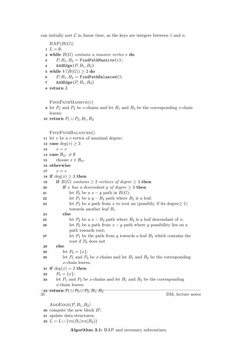
can initially sort C in linear time, as the keys are integers between 1 and n.

BAP(B(G))1 L = ∅;2 while B(G) contains a massive vertex v do3 P,B1, B2 = FindPathMassive(v);4 AddEdge(P,B1, B2)

5 while V (B(G)) ≥ 2 do6 P,B1, B2 = FindPathBalanced();7 AddEdge(P,B1, B2)

8 return L

FindPathMassive(v)9 let P1 and P2 be v-chains and let B1 and B2 be the corresponding v-chain

leaves;10 return P1 ∪ P2, B1, B2

FindPathBalanced()11 let v be a c-vertex of maximal degree;12 case deg(v) ≥ 313 x = v14 case B3+ 6= ∅15 choose x ∈ B3+16 otherwise17 x = v18 if deg(x) ≥ 3 then19 if B(G) contains ≥ 2 vertices of degree ≥ 3 then20 if x has a descendant y of degree ≥ 3 then21 let P0 be a x− y path in B(G);22 let P1 be a y −B2 path where B2 is a leaf;23 let P2 be a path from x to root an (possibly, if its degree≥ 1)

towards another leaf B1

24 else25 let P2 be a x−B2 path where B2 is a leaf descendant of x;26 let P0 be a path from x− y path where y possibility lies on a

path towards root;27 let P1 be the path from y towards a leaf B1 which contains the

root if P0 does not28 else29 let P0 = {x};30 let P1 and P2 be x-chains and let B1 and B2 be the corresponding

x-chain leaves;

31 if deg(x) = 2 then32 P0 = {x};33 let P1 and P2 be x-chains and let B1 and B2 be the corresponding

x-chain leaves;

34 return P1 ∪ P0 ∪ P2, B1, B2

AddEdge(P,B1, B2)30 compute the new block B′;31 update data structures;32 L = L ∪ {vx(B1)vx(B2)}

Algorithm 3.1: BAP and necessary subroutines.


Let us first FindPathBalanced. Note that x on line 17 is a critical vertex, if acritical vertex of degree ≥ 3 exists in B(G). If deg(x) = 2, then B(G) does notcontain vertices of degree ≥ 3 and, in particular, has exactly two leaves.

Now let us turn to line 18, and let us denote the root of B(G) with r. Assumefirst that x 6= r. If deg(r) ≥ 3 then we can choose P0 to be the B0 − x path. Ifdeg(B0) ≤ 2 and both sons y1 and y2 satisfy `r,y1 ≥ 2 and `r,y2 ≥ 2. Then we canroute P0 from x up to r, and then down in the direction of the (other) subtree having≥ 2 leaves. This will eventually hit in a vertex of degree ≥ 3.

Otherwise we know that the root r does not lie on a path between two vertices ofdegree ≥ 3. Does x have an ancestor of degree ≥ 3? We can check this in constanttime, comparing ` and `−v . If ` − `−v ≥ 2, then B(G) contains a vertex of degree≥ 3 which lies on the path from x to the root r. Finally if ` − `−v = 1, then B(G)contains another vertex of degree ≥ 3 if and only if Sv2+ 6= ∅, which can again bedecided in constant time.

The case x = r is even easier. B(G) has another vertex of degree ≥ 3 if and only ifSr2+ 6= ∅.To put it all together: we can in constant time decide in which direction we shouldlook for P0. Clearly the amount of time needed to actually find and constructP0 ∪ P1 ∪ P2 is proportional to the length of the resulting path.

Let G′ be the graph G + vx(B1)vx(B2). How does its block graph B(G′) dependon B(G)? We compute the new block B′ on line 30, its vertex set is the union ofsets of vertices of blocks which lie on P . If a c-vertex v lies on P and deg(v) ≥ 3,then v is also a c-vertex of B(G′) whose new degree has decreased by exactly 1. Ifdeg(v) = 2 then v is no longer a c-vertex of B(G′). Finally as P contains r, thenthe newly constructed block B′ serves as the root of B(G′).

We need to refresh auxiliary data structures on line 31 only for vertices of B(G′)which are descendants of B∗. Now if v 6∈ V (P ) then its auxiliary data is leftunchanged. If v is a c-vertex in V (B(G′))∩ V (P ), then the corresponding auxiliarydata can be computed in constant time. The data for B′ on the other hand takes timewhich is proportional to the length of P , which is up to a constant term proportionalto the difference |V (B(G)) − V (B(G′))|. This implies that we can solve the BAPproblem in linear time.

Theorem 3.5 Let G be an undirected, and let B(G) be its block tree. We can solvethe Biconnectivity Augmentation Problem in O(n+m) time.Even more, if B(G) is precomputed and has n′ vertices, then the algorithm BAPcomputes an augmenting set of edges F in O(n′) time.

Proof. As computing B(G) takes O(n+m) time, and since n′ = O(n), it is enoughto show the latter statement.

Both FindPathMassive and FindPathBalanced take time proportional to thelength P , their output. Also the routine AddEdge takes time, that is proportionalto the length of the input path P . Then there exist positive constants a and b, so


that the running time of FindPathBalanced, FindPathMassive, and AddEdgetakes at most a(|P | − 1) + b time.

What is the cumulative running time of BAP on an input graph G = G0? LetG0, G1, G2, . . . , Gk be the sequence of graphs obtained by inductively adding edgesbetween b-vertices of paths P1, P2, . . . , Pk, resulting in a 2-connected graph Gk. Thetotal running time is O((|P1| − 1) + (|P2| − 1) + · · ·+ (|Pk| − 1) + k), which is sincek = O(n′) equal to O(n′). �

3.2 Structure of 2-connected graphs

Let us now turn our attention to 2-connected graphs. An ear decomposition of agraph G is a sequence of graphs G1, G2, G3, . . . , Gk, so that

(ED1) G1 is a cycle,

(ED2) Gk = G, and

(ED3) Gi is a graph obtained from Gi−1 by attaching a path Pi between two verticesx and x′ of Gi−1.

The added path Pi is also called an ear , and can also be a single edge.

Theorem 3.6 Let G be an undirected graph. Then G admits an ear decompositionif and only if G is 2-connected.

Proof. Assume that G admits an ear decomposition: 2-connectivity of G can beshown by induction. Let G1, G2, G3, . . . , Gk−1, Gk = G be the ear decomposition ofG. Inductively we may assume that Gk−1 is 2-connected, as its ear decompositionis shorter. If G is not 2-connected, then G contains a cutvertex v. As Gk−1 is2-connected Gk−1− v is a connected graph. Hence also Gk−1− v ∪Pk. This impliesthat v is an internal vertex of Pk. This is also not possible, as G−v can be obtainedby attaching a pair of pendant paths to a connected graph Gk.

As G is 2-connected, the minimal degree of a vertex is at least 2, which impliesthat G contains a cycle subgraph G1. Assume that we have already constructed thesequence G1, G2, . . . , Gj . Assume there exists a vertex v ∈ V (G) \ V (Gj). As G isa 2-connected graph there exist v−V (Gj) paths Q,Q′ which share vertex v but areotherwise disjoint (and only meet V (Gj) in their endvertices). Their union Q ∪ Q′can be used as the next ear Pj+1. Hence we may assume that Gj is a spanningsubgraph of G. Now the missing edges from E(G) \E(Gj) serve at the final ears inthe ear decomposition of G. �

Let G be an undirected graph. An st-labeling (or also st-ordering) of G is a linearordering of its vertices v1, v2, . . . , vn, so that for every vertex vi, 1 < i < n, thereexist indices j < i and k > i, so that vi is adjacent to both vj and vk.


We can picture an st-ordering by arranging vertices of G on a real line, so that everyvertex, except the leftmost and the rightmost one, has a vertex both to the left andto the right of itself.

The origin of the name st-labeling comes from directed graphs. If we orient everyedge of G from a vertex of the lower label towards the vertex of the higher label, weobtain a dag with a single source s = v1 and a single sink t = vn.

Let us first state a nice property of an st-labeling of a graph G.

Proposition 3.7 Let v1, v2, . . . , vn be an st-labeling of G. Then for every i ∈{1, . . . , n−1} both induced subgraphs G[v1, . . . , vi] and G[vi+1, . . . , vn] are connected.

Proof. Fix i ∈ {1, . . . , n− 1} and let j ≤ i. Inductively can show that v1 and vj liein the same component: this is obviously true if j = 1, and is also true for biggervalues of j, as vj is adjacent to a vertex with a smaller index. The proof follows bysymmetry. �

Is there a relation between an st-labeling and an ear decomposition? Indeed, everyear decomposition can be transformed to an st-labeling, as we shall see in the proofof Theorem 3.8.

Does every graph admit an st-labeling? Clearly disconnected graphs do not admitst-labelings. Also not every connected graph admits an st labeling. Let G bea connected graph and assume that B(G) contains three leaf blocks B1, B2, B3.Now, being leaf blocks, Bi, i = 1, 2, 3, attaches to the rest of the graph through acutvertex bi. Assume that G admits an st-labeling v1, . . . , vn. We may without lossof generality assume that neither v1 nor vn are vertices of B1. Now let I = {i | vi ∈V (B1)} and let imin and imax be the smallest and largest indices in I, respectively.As b1 can only be identical to one of vimin or vimax , either vimin has no neighbor toits left or vimax has no neighbor to its right.

If G is a connected graph so that B(G) contains exactly 2 leaf blocks, then G canbe transformed into a 2-connected graph with an addition of a single edge. Thesegraphs do admit an st-labeling.

Theorem 3.8 Let G be a 2-connected graph and let xy ∈ E(G). Then G admits anst-labeling so that x = v1 and y = vn.

Proof. Let G1, G2, . . . , Gk = G be a fixed ear decomposition of G, so that xy ∈E(G1). We shall inductively construct linear orders of vertices of graphs in thedecomposition, and compute labels of vertices only with the final ordering L.

The x− y-Hamilton path represents the initial order of V (G1). Inductively assumethat we have constructed an ordering of Gi. Let xi, yi ∈ V (Gi) be the endverticesof the next ear Pi+1. We can insert the internal vertices of Pi+1 between L so thatevery internal vertex of Pi+1 lies in L between its neighbors in Pi+1 (not necessarilycontinuously). �


Let us finish with an algorithm for computing an st-ordering of a 2-connected graphusing Algorithm 2.2 DFSlow. Let G be a 2-connected graph, and xy a fixed edge.In order to construct an st-labeling with x the initial vertex and y the terminalone let us first compute both the starting times and low points start(v) and low(v)for every vertex v ∈ V (G), assuming the search starts at x moving to y next, i.e.start(x) = 1 and start(y) = 2. Let us denote the start time of the father of v bypred(v). As G is a 2 connected graph we have

(5) for every vertex v 6= x, y we have pred(v) > low(v),

as if pred(v) ≤ low(v) implies that pred(v) is a cutvertex in G since his son v hasits lowpoint low(v) at least as large as pred(v). Let us consider vertices accordingto their start times. Choose v 6= x, y and let us assume that the partial st-orderingL contains every vertex whose start time is strictly smaller than start(v). Then letus

extend L by putting (1) v between pred(v) and low(v) and also (2) next to pred(v).(3.2)

Let v 6= s, t. A v-lowpath is a v − low(v)-path following tree edges with a possiblefinal back edge. We claim that in the end (3.2) produces an st-labeling of the wholegraph G. We have to show that every vertex v 6= x, y has a neighbor both to itsleft and to its right, and we will do it by induction on the length of the v-lowpathP . If |P | = 1 then v is adjacent to both pred(v) and low(v), and thus has a leftand a right neighbor in the final ordering. If |P | > 2 let v′ be adjacent to v alongP . This implies that v′ is a son of v, low(v′) = low(v), and v′-lowpath P ′ is strictlyshorter than P . As v′ lies between v = pred(v′) and low(v′) = low(v) in the finalordering, both v′ and low(v) lie to the same side relative to v, and to the other sideas pred(v). Hence also v has both a neighbor to the left and a neighbor to the right.

There is an algorithmic caveat. In order to be able to add elements immediatelynext to a fixed element, the data structure containing the temporary linear orderingshould be a doubly linked list. But given two elements from a doubly linked listlow(v) and pred(v), how can we quickly (in constant time) decide which lies to theleft of the other?

There is a solution to the above problem by using signs of vertices: sign(v) = + (or−) indicates that a vertex u whose low(u) = v should be put in L before (or after)


v, respectively. A sign of a vertex may change in time, though.

STlabel(G, s, t)1 run DFSlow to compute start(v), low(v),2 and pred(v), so that start(s) = 1 and start(t) = 2;3 set sign(s) = − and L = [s, t];4 for v ∈ V (G) in the increasing start(.) order do5 if sign(low(v)) = + then6 insert v immediately after pred(v) in L;7 set sign(pred(v)) := −8 if sign(low(v)) = − then9 insert v just before pred(v) in L;

10 set sign(pred(v)) := +

11 return L

Algorithm 3.2: st-labeling algorithm

Theorem 3.9 The algorithm STlabel correctly computes L and does so in timeO(n+m).

Proof. Time complexity is easy, as DFSlow runs in O(n + m) time, and the restcan be done in O(n) time, provided we store L in a doubly linked list.

Let v be the current vertex on line 4 of STlabel. We claim that upon inserting vin L every proper ancestor u of v has a sign describing its relative positions to v: ifu is before v in L then sign(u) = −, and u lies after v then sign(u) = +.

Let v∗ = pred(v). Upon inserting v in L we have only adjusted the sign of v∗. Hencefor every ancestor u of v∗ its sign sign(u) describes its relative position to v∗ as well:sign(u) = − if and only if u lies before v∗ in L. Now low(v) is a proper ancestor ofv∗ and lies to the left of v∗ if and only if sign(low(v)) = −. In this case line 8 puts vimmediately to the left of v∗ which in turn implies that (1) low(v) is to the left of vand (2) sign(v∗) indicates the relative position of v∗ with respect to v, as claimed.

By symmetry the proof is finished. �


4 Planar graphs

4.1 Embedding as a drawing

Choose a graph G. We would like to draw G in the plane without crossings. But letus first tackle the simpler question on how to draw vertices and edges.

An arc in Σ is an embedding (injective continuous mapping) of an interval [0, 1] intoS, a simple closed curve is an embedding of S1 in Σ. We shall implicitly assumethat mappings are nice — they do not contain topological pathologies. We may forexample assume that an embedding is piecewise linear (provided Σ is equipped witha linear-space-like structure) or differentiable (if Σ is smooth).

A drawing of G in Σ is a mapping

D : V (G) ∪ E(G)→ Σ (4.1)

satisfying the following conditions:

(D1) for different vertices u, v ∈ V (G) we have D(u) 6= D(v), the restriction of Dto V (G) is injective,

(D2) for every edge e = uv ∈ E(G) its image D(e) is an arc whose endpoints areD(u) and D(v), and

(D3) there are no unnecessary intersections — if u is not an endvertex of e thenD(u) and D(v) are disjoint, and the only possible intersection of D(e) andD(f) is the image of their common endvertex.

We shall first focus on planar drawings where Σ = R2, and minutes later establisha connection with drawings in the sphere.

Graph G is planar if G admits a planar drawing D. A pair (G,D) is called a planegraph. Let us define D(G) as the union of images of vertices and edges of G andcall D(G) the drawing of G.

Given a fixed drawing, we shall informally identify G with its drawing and speak ofthe plane graph G.

A face of (G,D) is a connected component of Σ \ D(G). Informally faces can beobtained by cutting the surface Σ with scissors running along drawings of edges. Ina planar drawing, exactly one of the faces is unbounded, we shall call it the infiniteface. A face can be described with a facial walk — a sequence of vertices that weencounter by travelling along its boundary.

Let S2 denote the 2-sphere, set of points in 3-space at unit distance from the origin,and let N denote the north pole of S2 (the point (0, 0, 1)). We know that thestereographic projection ϕ maps S2 \N bijectively to R2 (the xy plane in 3-space).Let r be a one-way infinite ray originating in the north pole. If vs ∈ S2 \N , vr ∈ R2,and both lie in r, then ϕ(vs) = vr.


If (G,D) is a plane graph, then the mapping ϕ−1 ◦D is a drawing of G in the sphere(which misses N). Similarly if D′ is a drawing of G in the punctured sphere S2 \N ,then ϕ ◦D′ is a planar drawing of G.

Now let f∞ be the infinite face of (G,D). Now ϕ−1 ◦ D is a drawing of G in thesphere, and ϕ−1(f∞) is a face in the spherical drawing containing N . Let R be anarbitrary rotation of the sphere, and consider the mapping ϕ ◦R ◦ϕ−1 ◦D. We mayslightly perturb R (if necessary at all) so that the north pole is not the image of avertex or an edge. The set of facial walks has stayed the same, but the facial walkof f∞ may now describe a bounded face.

The above argument implies that the infinite face of a planar drawing f∞ is just aninconvenience (as every face can be made the infinite one if we rotate the sphericalprojection of the planar drawing). On the other it can be a feature of the drawing:if in some case we would like to pick a particular face from a planar drawing we canalways name it the infinite face.

4.2 Combinatorial embeddings

Let G be a plane graph, and let us choose an orientation — say clockwise — inthe plane. For every vertex v let πv denote the cyclic ordering of neighbors of v inthe clockwise (i.e. chosen orientation) ordering around v. The collection of all cyclicorderings {πv | v ∈ V (G)} is called rotation system of the drawing of G.

If uv ∈ V (G), then u′ = πv(u) is called the successor of u around v and symmetricallyu is the predecessor of u′ around v. The ordered triple [u′, v, u] is then also calledan angle. These terms have the following geometric interpretation. Choose a pointp on D(vu) very close to D(v). Rotating p (clockwise) around u will first intersectD(G) in a point of D(vu′).

Let v0v1 be an edge of G. The sequence v0v1v2 . . . vd−1 is a facial walk if

(F1) for every i = 1 ∈ {0, . . . , d−1} the triple [vi, vi+1, vi+2] is an angle (indices aretaken mod d) and

(F2) no angle is repeated, for i 6= j we have [vi, vi+1, vi+2] 6= [vj , vj+1, vj+2].

Condition (F1) implies that we follow a face along consecutive angles, and (F2)prevents of going around the face twice.

Let us look at the the cube graph Q3, with vertices V (Q3) = {1, . . . , 8}. The edgeset will implicitly defined by the rotation system


πv1 = (v2, v3, v5)πv2 = (v1, v7, v4)πv3 = (v1, v4, v5)πv4 = (v2, v6, v3)πv5 = (v3, v6, v8)πv6 = (v4, v7, v5)πv7 = (v2, v8, v6)πv8 = (v1, v5, v7)

In order to compute the facial walks (which in turn determine faces) let us followangles starting from every possible direction of an edge. Choose, for example v1v2.Now v4 is the predecessor of v1 around v2, as πv2(v4) = v1, hence [v1, v2, v4] is anangle. The following three angles are [v2, v4, v3], [v4, v3, v1], and [v3, v1, v2], and thenext angle [v1, v2, v4] is the repetition of the first one. Hence we obtain a facial walkv1v2v3v4.

The remaining facial walks are v2v1v8v7, v4v2v7v6, v4v6v5v3, v1v3v5v8, and v5v6v7v8.Observe that every edge appears exactly twice in the facial walks, once in eachdirection.

Similarly, given a collection of facial walks (a collection of walks in which every edgeexactly twice, once in each of the directions) determines the rotation system: on onehand we can determine the lists of neighbors of each vertex v, on the other hand wecan for each neighbor u of v determine its successor in the rotation system — weonly need to find the vertex u′ which immediately precedes v, u in the collection offacial walks.

It seems that the original choice of the orientation (clockwise or counter-clockwise)produces a different rotation system, and consequently a different set of faces. Weshall however declare these choices being equivalent: by reversing all cyclic orderingsin a rotation system has a consequence that the constructed facial walks all run indifferent directions.

This motivates us to define the combinatorial embedding of G as every structurethat uniquely determines both the rotation system and the set of facial walks in adrawing of G (up to a possible reversal).

Now a combinatorial embedding may not produce a planar drawing. Fortunately,there is only one criterion to meet. Provided that the combinatorial embeddingdetermines the correct number of faces (see Theorem 4.9) then it also determines adrawing in the plane.

Let us finish this subsection with a definition. Let f be a face of a drawing of aplanar graph G. The length of f , deg(f), is defined as the length of its facial walk.

4.3 Results from topology

Let us state a couple of mathematical (indeed topological) theorems. These resultsare surprising in the following way — they seem to be obviously true. Yet they


require deep (i.e. this is not freshman-year-mathematics) and technical proofs whichare way above our reach.

Theorem 4.1 (Jordan Curve Theorem) Let C be a simple closed curve in R2.Then R2 \C has exactly two connected components: the interior of C is the boundedcomponent and the exterior of C is unbounded. C is the boundary of both the interiorand exterior components.

Theorem 4.2 (Three arcs theorem) Let P1, P2, P3 be three arcs with commonendpoints x and y, and otherwise disjoint in R2. Let z1 and z2 be interior points ofP1 and P2, respectively. Let P be an arbitrary z1 − z2-arc, which lies in the sameconnected component of R2 \ (P1 ∪ P2) as P3. Then P ∩ P3 6= ∅.

4.4 Connectivity and planar graphs

Let G be a disconnected graph. Then G is planar if and only if every componentof G is planar, as disjoint components can be drawn in the plane independently, farapart. Hence we shall in the sequel limit ourselves to connected graphs.

Let G be a graph which is not 2-connected, and contains at least 3 vertices. Then Gcontains at least one cutvertex, and possibly also a cutedge. These play a particularrole in case G is planar.

Proposition 4.3 Let G be a plane graph.A vertex v is a cutvertex in G if and only if there exists a face f so that v appearsat least twice on its facial walk.An edge e is a cutedge in G if and only if there exists a face f ′ so that e is traversedexactly twice on a facial walk of f ′. In this case each direction of e is traversedexactly once.

Proof. Assume first that v is a cutvertex and let G1 be a component of G. Let uscolor all edges of G1 + v in red, and the rest of edges green. Now the local rotationπv determines a mixed angle (v0, v, v1), an angle in which the edge v0v is green andvv1 is a red edge. Let f be the face containing the angle (v0, v, v1) and observe thecolors of edges along its facial walk. They must change at least twice, and this canonly happen in v, as v is the only vertex incident with edges of both colors.

Assume that the facial walk of f enters v twice. Let (v0, v, v1) and (u0, v, u1) be thecorresponding angles. We can construct a simple closed curve C entering v betweenvv0 and vv1 and leaving between vu0 and vu1, which is otherwise disjoint with G.As no v0 − v1-path can pass through C \ {v}, vertices v0 and v1 lie in differentcomponents of G− v.

The edge-part of the proof can be done analogously. �

As 2-connected planar graphs do not contain cutvertices, we have the following easycorollary.


Corollary 4.4 Let G be a 2-connected planar graph, and let D be an arbitrarydrawing of G. Then every facial walk of (D(G) is a cycle.

Corollary 4.4 has itself a rather nice corollary (see, again). Facial cycles of D(G) canbe interpreted as subgraphs of G. On the other hand it is not true that the graph Gitself determines the set of facial cycles. Even a 2-connected graph can have severaldrawings in the plane, which in turn determine different collections of facial cyclesin each of the embeddings.

Consider the following scenario. Let G be a plane graph, and let x, y be a 2-separatorin G. This implies that we can find a simple closed curve C, passing through bothx and y and otherwise disjoint from G, so that both the interior and exterior of Ccontain vertices of G, respectively. We can now reflect the interior of C, keeping xand y fixed, in order to obtain a different embedding of G. This procedure is calleda Whitney flip.

Theorem 4.5 (Whitney) Let D1 and D2 be combinatorial embeddings of a 2-connected planar graph G. Then D2 can be obtained from D1 by a series of Whitneyflips.

Now a 3-connected graph contains no 2-separators, so no Whitney flips are possiblein an embedding of a 3-connected planar graph. This implies the following corollaryof Theorem 4.5.

Theorem 4.6 Let G be a 3-connected planar graph. Then G has a unique combi-natorial embedding in the plane.

Now Theorem 4.6 implies that in a 3-connected planar graph the collection of facialwalks (these are indeed cycles by Corollary 4.4) is uniquely determined. It is notsurprising that these can be described in a purely combinatorial way.

Theorem 4.7 Let G be a 3-connected planar graph. Then the collection of faces ofG is exactly the set of nonseparating induced cycles of G.

Proof. Assume G is drawn in the plane, and let C be a face of G (we shall alsoassume that C is not drawn as the infinite face so that its interior is empty). Letu, v be nonconsecutive vertices along C which are adjacent. Choose an u− v-arc inthe interior of C. Together with the edge uv it forms a simple closed curve whichseparates vertices of the two segments of C − v − u. This is not possible as G is a3-connected graph. Therefore C is induced.

Now let x, y 6∈ V (C). As G is 3-connected there exist three internally disjoint x− y-paths P1, P2, and P3. Now C lies in one of the regions bounded by two among thesepaths not containing the third, without loss of generality P1 ∪ P2. Hence C andP3 have no vertices in common and C does not separate x form y. As x, y werearbitrary this implies that C is not separating.


For the other direction observe that a nonseparating induced cycle C cannot con-tain vertices of G both in its interior and its exterior. Hence we may without lossof generality assume that its interior contains no vertices of G. As C is an inducedcycle its interior cannot contain edges of G either. Hence C is a face. �

A triangulation is a plane graph G in which every face is of length 3 (recall that Gcan have no parallel edges).

Proposition 4.8 Let T be a triangulation. Then T is 3-connected. Moreover if Sis a minimal separator in T , then S induces a cycle.

Proof. Let S be a minimal separator in T , and let T1 be a component of T −S. Letus replicate the trick by coloring edges. Let us color edges in T1 as well as edgesbetween S and T1 red, edges between vertices of S black, and remaining edges green.If |S| ≤ 2 then there exists a face f with an angle (u, s, x) where us is a green edgeand sx is a red edge. As x and u are not adjacent, |f | ≥ 4, which is a contradiction.

Let S be a minimal separator in T . Now Proposition 4.15 implies that T − S con-tains exactly two components T1 and T2. Let us color edges of T in three colors red,green, and black as above, and let us again use the fact that no angle contains ared and a green edge. Hence each vertex s ∈ S is incident with at least two blackedges. This implies that G[S] contains a cycle. Let C1 be the shortest cycle of G[S]so that both its interior and exterior contains a vertex of G. If V (C1) 6= S, then wehave a contradiction with minimality of S. Let ss′ ∈ E(G) be an edge between twononconsecutive vertices of C1. Now C1 + ss′ divides R2 into three regions so that(i) at least two contain vertices of G (as C1 is a separating cycle) and at (ii) leasttwo are empty as the both short cycles of C1 + ss′ are nonseparating, which is acontradiction. �

4.5 Euler formula

Let G be a plane graph. Let us with F (G) denote the set of faces of G.

Theorem 4.9 (Euler formula) Let G be a connected plane graph. Then

|V (G)| − |E(G)|+ |F (G)| = 2

Proof. Choose a spanning tree T of G. Now V (T ) = V (G), E(T ) = V (T ) − 1 =V (G)− 1 and F (T ) = 1, hence

|V (T )| − |E(T )|+ |F (T )| = |V (G)| − (|V (G)| − 1) + 1 = 2, (4.2)

in other words, Euler formula holds for the spanning tree T . Now adding an edge ofE(G) \E(T ) has the following effect: number of vertices does obviously not change,


and the number of edges increases by one. An addition of a new edge (it is nota cutedge as together with T it forms a cycle) divides an existing face into a pairof new faces, and thus increases the number of faces by one as well. Hence Eulerformula holds by induction on the number of edges in E(G) \ E(T ) for the originalgraph G as well. �

Now Euler formula effectively bounds the number of edges in a planar graph:

Proposition 4.10 Let G be a (planar) plane graph with at least 3 vertices. Then

1. |E(G)| ≤ 3|V (G)| − 6, and

2. |E(G)| = 3|V (G)| − 6 if and only if G is a triangulation.

Proof. Assume G is drawn in the plane, and let us sum the lengths of its faces.

2|E(G) =∑

f∈F (G)

deg(f) ≥ 3|F (G)|

The first equality follows as every edge appears exactly twice along facial walks, andthe second inequality as the length of each face is at least 3. Note that equalityarises if and only if G is a triangulation, both in the above and consequently belowcomputation.

3|V (G)| − 6 = 3|E(G)| − 3|F (G)| ≥ 3|E(G)| − 2|E(G)| = |E(G)|

�

Let us continue with a technical lemma.

Lemma 4.11 Let G be a plane graph. Then G is bipartite if and only if all facialwalks are of even length.

Proof. Clearly no closed walk in a bipartite graph can be of odd length. For theconverse, let us choose a cycle C in G. Now |C| has the same parity as the sum ofparities of lengths of faces, which are contained in the interior of C. This followseasily by induction on the number of faces in the interior of C. �

Proposition 4.12 Let G be a bipartite (planar) plane graph with at least 3 vertices.Then

1. |E(G)| ≤ 2|V (G)| − 4, and

2. |E(G)| = 2|V (G)| − 4 if and only if G is a quadrangulation.


A quadrangulation is a plane graph whose faces are all of length 4. The proof ofProposition 4.12 can be settled in the very same manner as the proof of Proposi-tion 4.10. The only difference is that every face in a bipartite plane graph has to belonger than 4.

We have nevertheless devised the necessary tools to find first examples of nonplanargraphs.

Proposition 4.13 K5 and K3,3 are not planar graphs.

Proof. K5 has 5 vertices and 10 edges, and K3,3 is a bipartite graph with 6 verticesand 9 edges. By Proposition 4.10 an Proposition 4.12 their numbers of edges aretoo big for them to be planar. �

Let G be a planar graph. Clearly the following three operations preserve planarity:deleting vertices, deleting edges, and subdividing edges (replacing a single edge witha longer path). All these operations can namely be carried out not only on the graphG itself, but also on its drawings.

Hence the class of all planar graphs is closed under taking subgraphs and also undertaking subdivisions.

There is another operation which preserves planarity, the edge contraction. Lete = uv be an edge in G. Let Nu,v be the set of vertices of G − u − v which areadjacent to at least one of u, v. The graph G/e is obtained form G − u − w byadding a new vertex xuv and making it adjacent to every vertex of Nu,v. We saythat G/e is obtained from G by contracting e.

If G is a plane graph, then the drawing of G/e can be obtained by drawing xuv on amidpoint of the edge uv. The xuv−Nu,v edges can be drawn simultaneously withoutcrossings in the vicinity of uv and edges incident with either u or v.

We call a graph H a minor of G, if H can be obtained from G by a series of vertexdeletions, edge deletions, and edge contractions.

By above description the class of planar graphs is also minor closed .

It is therefore not surprising that we can characterize planar graphs both in termsof forbidden subdivisions and also forbidden minors. What is surprising is the factthat the sets of obstructions is the same in both cases, and that K5 and K3,3 areindeed the smallest nonplanar graphs.

Theorem 4.14 (Kuratowski, Wagner) G is planar if and only if

1. G does not contain a subdivision of K5 or K3,3 (or equivalently)

2. G does not contain a K5 or K3,3 as a minor.

We shall skip the proof.

Finally let us state and prove a proposition on the number of components relativeto a small separator.


Proposition 4.15 Let G be a 3-connected planar graph, and let S be a minimalseparator. Then G− S contains exactly two connected components.

Proof. Assume that G − S contains three connected components G1, G2, and G3.Let us contract G1, G2, and G3 to single vertices g1, g2, g3, respectively (we can dothat inductively, as contracting a single edge reduces the vertex-count by one). As Sis a minimal separator, every vertex si ∈ S has a neighbor in each of the componentsof G − S. Hence every vertex of S is adjacent to g1, g2, and g3 in the contractedgraph. As |S| ≥ 3 we obtain a K3,3-minor in G, which is absurd. �

4.6 Dual graphs

Let G be a (connected) plane graph. We can construct the dual graph G∗ in thefollowing way:

1. for every face f ∈ F (G) put a vertex f∗ ∈ V (G∗) in the interior of f , and

2. for every edge e ∈ E(G) so that faces f1 and f2 contain e in their respectiveboundaries, the vertices f∗1 and f∗2 are adjacent via an edge e∗ in G∗.

The edge e∗ is also called the dual edge of e, which also means that there exists abijective correspondence between edges of G and those of G∗.

Dual graph G∗ appears to be a purely geometric concept. Yet it turns out to beof a different, combinatorial intact, flavor. Minimal edge-cuts in G correspond tocycles of G∗ and vice-versa. Cycles in G correspond to minimal edge cuts of G∗.This is due to Jordan Curve Theorem 4.1. A cycle C in G is a simple closed curvein the plane (sphere) and separates R2 into exactly two connected components, theinterior and exterior of C. Let V ∗1 be the set of vertices of G∗ (i.e. faces of G) whichlie in the interior of C, and V ∗2 be the set of vertices of G∗ which lie in exterior ofC. Now every V ∗1 − V ∗2 -path in G∗ crosses C, and hence uses an edge e∗ which is adual edge of some edge e ∈ E(C). Hence the collection of dual edges of E(C) is acut in G∗. It is indeed a minimal cut, as the end vertices of each edge e∗ ∈ E∗(C)lie in different components of R2 \ C.

It is easy to argue that G∗∗ = G, if G is a connected plane graph.

How are deletion and contraction of an edge in G and its dual G∗ related? Thedeletion of an edge e in E(G) merge the faces f1, f2 on either side of G into asingle face f1,2. The same effect can be produced in G∗ by contracting its dual edgee∗ = f∗1 f

∗2 . And conversely, contracting an edge in G has the same effect as deleting

its dual edge e∗ in G∗.

Hence contraction and deletion of edges form a pair of dual operations. The execu-tion of one operation in one of the graphs has exactly the same effect (as effect onthe pair of graphs, the original and its dual) as executing the other operation in thedual graph.


5 Discharging technique

5.1 Consequences of Euler formula

Let G be a connected plane graph. Euler formula (Theorem 4.9) implies severalstructural results for planar graphs.

Proposition 5.1 Let G be a plane graph.

• G contains a vertex of degree ≤ 5,

• if δ(G) = 5 then G contains at lest 12 vertices of degree 5.

Proof. If δ(G) ≥ 6, then summing vertex degrees implies that 2|E(G)| =∑

v∈V (G) deg(v) ≥6|V (G)| which in turn contradicts the fact that |E(G) ≤ 3|V (G)| − 6, see Proposi-tion 4.10.

Further we may assume that G is a maximal planar graph (i.e. a trinagulation) asaddition of edges cannot increase the number of vertices of small degree, and alsocannot decrease the minimum degree. Let n5 denote the number of vertices of degree5 in G, and let n6+ denote the number of vertices of larger degree in G.

Then 2|E(G)| =∑

v∈V (G) deg(v) ≥ 5n5 + 6n6+ . By Proposition 4.10 the expression2|E(G)| ≤ 6|V (G)| − 12 = 6n5 + 6n6+ − 12. This implies that n5 ≥ 12. �

A graph G is called k-degenerate if we can obtain an empty graph by repetitivelydeleting vertices of degree ≤ k starting from G. Equivalently stated, every subgraphof G has a vertex of degree ≤ k. An easy consequence of Proposition 5.1 is thatplanar graphs are 5-degenerate. Starting with a planar graph, deleting vertices ofdegree ≤ 5 will ultimately lead to the empty graph.

Proposition 5.2 Let G be a planar graph with n vertices. Then∑e=uv∈E(G)

min{deg(u),deg(v)} ≤ 10|E(G)| = O(n)

Proof. Let us number vertices v1, v2, v3, . . . , vn, so that vi has smallest degree (whichis ≤ 5) in G[vi, . . . , vn]. Now∑

e=vkv`∈E(G)

min{deg(vk),deg(v`)}

≤∑

e=vkv`∈E(G)

deg(vmin{k,`})

=

n∑i=1

deg(vi) · |{j | j > i and vivj ∈ E(G)}|

≤n∑i=1

5 deg(vi) = 10|E(G)| = O(n),


as the equality between second and third lines follows by counting the number ofedges, so that vi is their endvertex with the smaller index. �

5.2 Triangulating a plane graph

One of the basic problems is turning a planar/plane graph G into a triangulationby adding edges. Let G be a planar/plane graph with n ≥ 3 vertices and m edges.If m < 3n− 6 then at least one of the faces f in an arbitrary drawing of G (in caseG is not actually a plane graph, but merely a planar one) has length ≥ 4. Picka drawing of G and let f be a long face of deg(f) = k ≥ 4. Let v1v2v3 . . . vk beits facial walk. By adding an edge v1v3 in the interior of face f we have increasedthe total number of edges by one, which is a single step towards making all faces oflength 3. But there is a catch, the edge v1v3 might have already been present in theoriginal graph, lying in the exterior of face f . As we do not want parallel edges wehave to be a bit more careful.

triangulate(G)1 while G contains a face f of length deg(f) = k ≥ 4 do2 let v0 be a vertex of smallest degree along f ;3 if v0 has a nonconsecutive neighbor vi along f then4 foreach j ∈ {i+ 1, i+ 2, . . . , k − 1} do5 add edge v1vj6 foreach j ∈ {2, 3, . . . , i− 1} do7 add edge vi+1vj8 else9 foreach j ∈ {2, 3, . . . , k − 2} do

10 add edge v0vj

Algorithm 5.1: triangulate(G)

Proposition 5.3 Let G be a 2-connected plane graph. Then Algorithm 5.1 correctlycomputes a plane triangulation TG so that G is a spanning subgraph of TG.

Proof. It is easy to see that in either of if-cases on line 3 the algorithm triangu-lates the long face f , and the outer while loop takes care that every long face istriangulated upon finishing.

We only need to argue that no parallel edges are inserted in the run. This is clear if v0is not adjacent to another vertex of f , apart from the consecutive neighbors along f .On the other hand if v0vi is an edge and 2 ≤ i ≤ k−2 then by Theorem 4.2 no pair ofvertices x, y, which lie on different segments of f−v0−vi can be adjacent. Hence theinserted edges on lines 5 and 7 do not form parallel pairs with existing edges. �

Can we triangulate a plane graph G which is not 2-connected in the first place?There are some additional technical difficulties as facial walks in a plane graph


which is not 2-connected can have repeated vertices. Rather than specifying a moregeneral version of Algorithm 5.1 which would work on a larger class of input graphslet us describe a tool which works in a plane graph G having cutvertices.

Let G be a plane graph and v its cutvertex. Let πv be the local rotation of neighborsaround v in G. Assume that v1 is a predecessor of v2 around v, πv(v1) = v2. Thenadding the edge v1v2 to G, adjusting πv1 and πv2 , so that v is the predecessor of v1around v2 and that v2 is the predecessor of v around v1 produces a plane graph G′

with one block less in its block-tree. By applying the analogous operation on all pairsof predecessor-successor from different blocks, and iteratively over all cutvertices ofG we obtain a plane 2-connected supergraph G′ of G, so that V (G′) = V (G).

What we shall care next is the time complexity of Algorithm 5.1. Observe thatfor a connected planar graph we have |V (G)| − 1 ≤ |E(G)| ≤ 3|V (G)| − 6. Thisimplies that the number of vertices and the number of edges are of the same orderof magnitude and hence O(n) = O(m) if we use n and m for the numbers of verticesand edges, respectively.

Theorem 5.4 Let G be a 2-connected plane graph. Then Algorithm 5.1 runs inlinear time.

Proof. Let f1, f2, . . . , fk be the list of long faces in G = G0. Let Gi denote thegraph obtained after triangulating the faces f1, . . . , f i by Algorithm 5.1.

In order to find the vertex v0 of smallest degree along f ` we have to traverse allvertices of f ` which takes O(|f `|) time. In this process we also flag every vertexof f `, so that we can check for possible neighbors of v0 along f ` in O(degG`−1

(v0))

time. Adding the edges in order to triangulate f ` takes time O(|f `|) and so doesremoving the flags of vertices along f ` at the end.

Hence the total time complexity is equal to

O

(k∑i=1

deg(f i)

)+O

(k∑i=1

minv∈f i{degGi−1

(v)}

). (5.1)

Let us estimate the terms separately. On one hand

k∑i=1

deg(f i) ≤∑

f∈F (G)

deg(f) = 2|E(G)|.


The other sum proves to be more troublesome:

k∑i=1

minv∈f i{degGi−1

(v)}

≤k∑i=1

minv∈f i{degGk

(v)}

≤k∑i=1

1

4

∑e=uv∈E(f i)

min{degGk(u), degGk

(v)}

≤∑

e=uv∈E(Gk)

min{degGk(u), degGk

(v)} = O(|V (Gk)|)

The first inequality holds as degrees of vertices grow as we triangulate faces, thesecond as each face f i is of length ≥ 4 (note that f i is a cycle in Gk). The lastinequality follows as every edge e ∈ E(Gk) belongs to at most two long faces of G,finally we apply Proposition 5.2.

Hence (5.1) is the sum of two terms of order O(n) and the proof is complete.�

5.3 Discharging method

Our first results in this writeup have established the fact that every planar graphcontains a vertex of bounded degree (at most 5 was the best possible bound). Doesevery planar graph contain an edge so that the sum of degrees of its endvertices isbounded as well? This turns out to be false, as every edge in K2,n (which is a planargraph) is adjacent with a vertex of large degree. However, if one limits to planargraph without vertices of degree ≤ 2, then we have an appropriate result.

Theorem 5.5 (Kotzig) Let G be a planar graph with δ(G) ≥ 3. Then G containsan edge e = uv so that deg(u) + deg(v) ≤ 13. Moreover if both deg(u) ≥ 4 anddeg(v) ≥ 4, then also deg(u) + deg(v) ≤ 11.

Proof. Let e = uv ∈ E(G) and let us assume that deg(u) ≤ deg(v). Let us calle = uv light if deg(u) = 3 and deg(v) ≤ 10 or deg(u) ≥ 4 and deg(v) ≤ 11− deg(u).

Assume that the theorem is false, and let G be a minimal counterexample: G is aplanar graph without light edges, that has the smallest possible number of verticesand biggest possible number of edges. Let us draw G in the plane.

We claim that every face of G is a triangle. Otherwise G has a face f of length≥ 4. Now f contains two nonconsecutive vertices u, v of degree ≥ 6 (otherwise twoconsecutive vertices have degree ≤ 5 which yields a light edge). Now G + uv is aplane graph without light edges as the newly added edge is not light, and contradictsthe minimality of G. (Note that the added edge might produce a graph with parallel


edges, but G+uv still has a drawing without faces of length 2, which in turn implies|E(G+ uv)| ≤ 3|V (G+ uv)| − 6.)

Now let us apply the discharging argument . We shall assign initial charge to verticesand faces of G. This charge will be redistributed in the graph, but the total chargeshall remain the same. In the end we shall obtain a contradiction: the structure ofthe graph G (in our case the lack of light edges) shall contradict the final distributionof charge.

Let v ∈ V (G). Its initial charge c0(v) = deg(v) − 6. If f is a face of G, then letc0(f) = 2 deg(f)− 6 = 2 · 3− 6 = 0. Now the total initial charge equals∑

v∈V (G)

c0(v) +∑

f∈F (G)

c0(f) (5.2)

=∑

v∈V (G)

(deg(v)− 6) +∑

f∈F (G)

(2 deg(f)− 6)

=∑

v∈V (G)

deg(v)− 6|V (G)|+ 2∑

f∈F (G)

deg(f)− 6|F (G)|

= 2|E(G)| − 6|V (G)|+ 4|E(G)| − 6|F (G)|= −6(|V (G)| − |E(G)|+ |F (G)|) = −12.

Let us call u a vertex of small degree if deg(u) ≤ 5, and let us call vertices of degree≥ 7 vertices of large degree. We shall redistribute charge in the discharging processaccording to the following rule.

Rule: Let uv ∈ E(G) and let u be a vertex of small degree. Then v sends v charge6−deg(u)deg(u) .

After applying the Rule let c1(V ) denote the final charge of a vertex. If f is a facethen c1(f) = c0(f) as the rule only transfer charges between vertices.

Observe first, as no edge is light, that a vertex of small degree u can only be adjacentto vertices of large degree. Hence u receives 6−deg(u)

deg(u) from each of its neighbors, and

c1(u) = c0(u) + deg(u) · 6− deg(u)

deg(u)= (deg(u)− 6) + (6− deg(u)) = 0.

If deg(v) = 6, then c1(v) = c0(v) = 0, as vertices of degree 6 do not play a role indischarging.

Now let w be a vertex of large degree k. As every face of G is a triangle, no twoconsecutive (around w) neighbors of w can be of small degree. Hence w can onlysend charge to at most bk2c neighbors.

If deg(w) = 7, then every neighbor of w has degree ≥ 5. Therefore c1(w) ≥ c0(w)−b72c

15 = 1− 3

5 ≥ 0.

If deg(w) = k ∈ {8, 9, 10} then every neighbor of w has degree ≥ 4. This impliesthat c1(w) ≥ c0(w)− bk2c

12 = (k − 6)− bk2c

12 ≥ 0.


Finally if deg(w) = k ≥ 11 then c1(w) ≥ c0(w)− bk2c = (k − 6)− bk2c ≥ 0

Now the total final charge is on one hand equal to −12 and is nonnegative in theother. This contradicts the fact that G has no light edges. �

5.4 Colorings of planar graphs

A (vertex)-coloring of G is a mapping

c : V (G)→ N,

so that for every pair of adjacent vertices u, v we have c(u) 6= c(v). A coloringshould necessarily color neighboring vertices with different colors. A k-coloring is acoloring into {1, 2, . . . , k}, and the smallest k for which there exists a k-coloring ofG is called the chromatic number of G, χ(G).

The notorious Four color theorem states that we can color vertices of an arbitraryplanar graph with no more than 4 colors. Let us state it without proof.

Theorem 5.6 (Four color theorem) Every planar graph G satisfies χ(G) ≤ 4.

Four color theorem is the optimal result, K4 is a planar graph and χ(K4) = 4. It ishowever possible to give short proofs of weaker results.

It is easy to see that χ(G) ≤ 6 for every planar graph G. Namely, every planargraph is 5-degenerate. This implies that we can construct an ordering v1, v2, . . . , vnof vertices ofG so that vi has degree≤ 5 inG[vi, vi+1, . . . , vn], see Proposition 5.2. Byrefreshing the set of vertices of degree ≤ 5 in the remaining graph we can constructthe sequence in linear time. Finally we color vertices of G greedily in the reverseordering vn, vn−1, . . . , v1, by coloring vi by the smallest color from {1, 2, 3, 4, 5, 6}which is not already used on colored neighbors of vi.

Constructing a 5-coloring of a planar graph is a bit more technical. At least threedifferent approaches exist. Historically, using Kempe chain argument predates bothcoloring by contraction and a list coloring argument of Thomassen 6.6.

Let us briefly explain the former two approaches, and let us leave Thomassen’s listcoloring idea for the next section, where it will be studied in greater detail.

Both Kempe-chain and contraction argument choose a vertex of smallest degreev ∈ G, and first recursively construct a coloring of G − v. If deg(V ) ≤ 4, then the5-coloring c′ of G − v can be extended to a 5-coloring of v. Hence we may assumethat deg(v) = 5, and that the neighbors of v in G are v1, v2, v3, v4, v5, with indicesmatching the local rotation around v.

Now if the coloring c′ does not use five different colors for v1, . . . , v5, again c′ canbe extended to v. Hence we may (without loss of generality) assume that c′(vi) = i.Observe the component C1,3 of G induced by vertices of colors 1 and 3 which containsv1. We can recolor vertices of C1,3 by changing colors 1 and 3 within C1,3, this


procedure is called a Kempe change. If we are lucky and v3 6∈ C1,3 then the changeresults in exactly four colors 2, 3, 4, 5 being used on neighbors of v. Otherwise there isa v1−v3 path consisting entirely of vertices colored with colors 1 and 3 in G−v, thisis a Kempe chain. Now a Kempe-chain between v1 and v3 implies that vertices v2and v4 do not lie on a path consisting of vertices of colors 2 and 4 only. Hence we canrecolor the component C2,4 containing vertex v2, and again construct a 5-coloringof G− v using 4 colors on neighbors of v.

The contraction argument on the other hand preemptively constructs a 5-coloringc′ of G− v which only uses ≤ 4 colors on v1, . . . , v5. Observe that it is not possiblethat both v1v3 ∈ E(G) and v2v4 ∈ E(G). We can assume that v1v3 6∈ E(G). NowG′ = G− v + v1v3/v1v3 is a planar graph in which vertices v1 and v3 are identified.A 5-coloring c′ of G′ can be identified with a 5-coloring of G− v in which vertices v1and v3 are assigned the same color. Again this implies that v1, . . . , v5 use at most 4different colors, so c′ can be extended to a 5-coloring of G.

However simple the above arguments are, they cannot be turned into a linear-timealgorithm. The Kempe chain approach needs a possible recoloring of sizable portionsof G, which can only be proven to take quadratic time altogether. The contractionargument can be turned into a linear-time algorithm by increasing the number ofdifferent contraction types — preformed not only at vertices of degree ≤ 5, but alsoat vertices of degree 6.

If we restrict ourselves to smaller classes of planar graphs, we can prove betterbounds. On one hand chromatic number drops by one if we forbid triangles.

Theorem 5.7 (Grotzsch) Let G be a planar graph without triangles. Then χ(G) ≤3.

On the other hand we achieve the same bound by keeping triangles and forbiddingshort cycles of several other lengths.

Theorem 5.8 Let G be a planar graph without cycles of lengths 4,5,6,7,8,9. Thenχ(G) ≤ 3.

Proof. Let us start with a minimal counterexample: let G be a planar graph withoutcycles of lengths 4,5,6,7,8,9, let χ(G) > 3, and let G have the smallest possiblenumber of vertices (we are not concerned with the number of edges).

As G is a minimal counterexample we may assume that every proper induced sub-graph of G is 3-colorable. Let us first state some easy properties of G:

1. G has no vertices of degree ≤ 2.

Assume to the contrary that G has a vertex v of degree ≤ 2. By minimality G− vadmits a 3-coloring. Now neighbors of v might use at most deg(v) ≤ 2 differentcolors, hence there exists a free color for v, and a 3-coloring of G−v can be extendedto the whole G.


2. G is 2-connected.

Assume that v is a cutvertex of G and let G1 be a component of G−v. By minimalitythere exist 3-colorings of both G1+v and G−G1, and these 3-colorings can be mergedto a 3-coloring of G, after possibly shifting colors of G1.

Now let us start with discharging. Let v be a vertex of G, its initial charge c0(v)is equal to deg(v) − 6. Similarly let c0(f) = 2 deg(f) − 6 for every face f ∈ F (G).Initial charges of vertices are compiled in the following table:

deg(v) 3 4 5 6 7 8 9 . . .

c0(v) −3 −2 −1 0 1 2 3 . . .

Recycling the computation of (5.2) we have∑v∈V (G)

c0(v) +∑

f∈F (G)

c0(f)

=∑

v∈V (G)

(deg(v)− 6) +∑

f∈F (G)

(2 deg(f)− 6) = −12.

Observe that there does not exist a pair of triangles which share a common edge, asthese would give rise to a cycle of length 4.

We shall redistribute charge from positively charged faces to vertices of small degreeaccording to the following rules:

Rule 1a: Let v be a vertex of degree 3. If v is incident with three long faces then eachface sends charge 1 to v.

Rule 1b: Let v be a vertex of degree 3. If v is incident with one triangle then each ofthe remaining two long faces sends charge 3

2 to v.

Rule 2a: Let v be a vertex of degree 4. If v is incident with four long faces then eachface sends 1

2 to v.

Rule 2b: Let v be a vertex of degree 4. If v is incident with two triangles then each ofthe remaining two long faces sends charge 1 to v.

Rule 2c: Let v be a vertex of degree 4 which is incident with exactly one triangle t.Then the two long faces which are adjacent to t send v charge 1

2 . The longface antipodal to t sends v charge 1.

Rule 3: Let v be a vertex of degree 5 and f a long face incident with v. Then f sendscharge 1

2 to v.

Let us first describe a reducible configuration, a graph which cannot appear in aminimal counterexample G.

Let GR be a graph on vertex set {ui, vi, zi | 0 ≤ i ≤ 4} so that zi is adjacent toui and vi, and vi is also adjacent to ui−1 and ui (all indices are taken modulo 5).


The vertices {ui, vi | 1 ≤ i ≤ 5} induce the so called inner cycle of length 10, andvertices zi are pasted as tips of triangles on alternate edges of the 10-cycle. The set{z0, . . . , z4} is the set of vertices of attachment of GR.

We claim that

• G does not contain GR as a subgraph, so that vertices of the inner cycle havedegree 3 in G(we allow additional edges emanating from attachment vertices).

Assume that G contains GR as a subgraph so that the vertices of the inner ring allhave degree 3 in G. Let G′ be obtained from G by deleting vertices of the innercycle. As G is a minimal counterexample, there exists a 3-coloring c′ of G′. We willshow hot to extend c′ to vertices of the inner ring.

Assume first that c′ uses at most two colors on attachment vertices z0, . . . , z4, withoutloss of generality these colors are 1 and 2. Let us use color 3 for every vertexui, 0 ≤ i ≤ 4, and finally let us color every vertex vi with color 3− c′(zi).If, on the other hand, c′ uses all three colors on all attachment vertices, then we maywithout loss of generality assume that z0 is the only attachment vertex colored withcolor 3. Now let us color vertices v1, v2, v3, v4 with color 3. Next we color verticesu1, u2, u3 with color 1 or 2 which is not present at z1, z2, z3, respectively. Finallylet us color vertices u4, v0, u0 in this order with colors 1 and 2. In this order theneighbors of a vertex currently being colored use exactly two colors, leaving one ofthe colors free.

Finally let us analyze the discharging procedure. Let c1 : V (G)∪ F (G)→ R denotethe final charge of vertices and faces of G.

Let v be a vertex. If deg(v) ≥ 6, then c1(v) = c0(v) ≥ 0. If deg(v) ≤ 4, thenc1(v) = 0, as Rules 1a, 1b, 2a, 2b, and 2c effectively discharge a vertex of degree≤ 4 and also cover every possible arrangement of long faces around v (note that notwo triangles share a common edge).

If deg(v) = 5, then v lies on at least three faces of length ≥ 5, hence its final chargec1(v) is at least 1

2 .

Let us now estimate the final charges of faces. If deg(f) = 3, then c1(f) = c0(f) = 0.As G is 2-connected every face of G is a cycle, and since G has no cycles of lengths4, . . . , 9, every face of G has length ≥ 10.

Now a face can send at most 32 to each vertex incident with f . If deg(f) ≥ 12, then

c1(v) ≥ c0(v)− 32 deg(v) = 2 deg(v)− 6− 3

2 deg(v) ≥ 0.

Let deg(f) = 11. Now c0(f) = 16 = 10 · 32 +1. Now c1(f) < 0 implies that f has sent32 to every vertex along f using Rule 1b. This in turn implies that (1) all verticesalong f have degree 3, and (2) every vertex v ∈ f is incident with a triangular face.Hence every second edge along f is incident with a triangle, which is absurd, as fhas odd length.

Let deg(f) = 10. Now c0(f) = 14 = 8 · 32 + 2 · 1 = 9 · 32 + 12 . We shall study all

possibilities for which c1(f) < 0. Let k1 be the number of vertices of degree ≥ 4


along f . If k1 ≥ 2, then c1(f) ≥ 0, as there exist at least two vertices that receiveat most 1 from f .

Assume next that f is incident with a vertex v of degree d ≥ 4. If d ≥ 5, then fsends at most 9 · 32 + 1

2 charge away, which implies c1(f) ≥ 0. Hence v has degree4 and v receives charge 1 from f . Let e1 and e2 be edges incident to both v andf . The faces adjacent to f along e1 and e2 are either both triangles or none is atriangle, as v receives charge 1 form f using either Rule 2b or Rule 2c. As all othervertices along f have degree 3 the parity of f implies that some vertex u along f isnot adjacent to a triangle. Now f sends charge 1 to u as well and c1(f) ≥ 0.

As the last instance let us consider the case where all vertices along f have degree3. If f is adjacent to ≤ 4 triangles, then f sends charge 1 to at least two vertices.As f cannot be consecutively adjacent to a pair of triangles (these would make a4-cycle) the number of triangle neighbors of f is bounded above by 5. But this isimpossible as 5 triangles adjacent to a face of length 10 whose vertices are of degree3 forms a reducible configuration GR. We infer that c1(f) ≥ 0 in all cases.

Thus we have arrived in contradiction as the total terminal charge is negative.�


6 List coloring of planar graphs

Ordinary vertex coloring allows for every vertex v the same palette of colors, fromwhere the color of v can be chosen from. In a more general setting we could havechosen palettes of colors for each vertex individually, and requiring that each vertexis assigned a color from its own palette — and still keeping the condition thatadjacent vertices are assigned different colors.

Formally, let G be a graph. We shall call a mapping

L : V (G)→ PN

a list assignment , and call L(v) the list of admissible colors for v.

Given L we say that G is L-list-colorable, if there exists a coloring c of G so that

c(v) ∈ L(v)

for every v ∈ V (G). In other words, as c is a coloring adjacent vertices have to getdifferent colors, and each vertex has to be assigned a color from its own list.

Now if G is L-list-colorable for every list assignment L satisfying |L(v)| ≥ k for everyv ∈ V (G), then we say that G is k-choosable. The choice number of G, ch(G), isthe smallest k for which G is k-choosable.

6.1 Basic properties

Consider the list assignment which is constant — every vertex v of G is assigned thesame list L(v). Clearly the critical information is the order of |L(v)|, and an L-list-coloring can be identified with a |L(G)|-coloring. Hence the list-coloring-problemis a generalization of the ordinary (vertex) coloring problem, and we also have thefollowing relation.

Proposition 6.1 For every G we have χ(G) ≤ ch(G).

But is there a difference between these two types of coloring? Consider the 6-cycle v1, v2, v3, v4, v5, v6, with the additional edge (main diagonal) v1v4, togetherwith the list assignment L(v1) = L(v4) = {a, b}, L(v2) = L(v5) = {a, c}, andL(v3) = L(v6) = {b, c}. Let us temporarily disregard the diagonal edge. Observethat choosing color a for v1 forces a unique extension of colors to the remainingvertices. Similarly, setting c(v1) = b forces a unique extension to the other verticesas well, the argument follows the other direction of the cycle. In either of cases weinfer that c(v1) = c(v4) are the same (and by analogy the same relations hold forcolors of other pairs of antipodal vertices). As v1 and v4 are adjacent we infer thatour graph is not L-list-colorable and consequently not 2-choosable. On the otherhand it is bipartite.

Form this discussion it follows that ch(G) can be strictly larger than χ(G). In fact,the difference can be arbitrarily large.


Proposition 6.2 For every k there exists a graph G so that ch(G)− χ(G) ≥ k.

Proof. Take the highly nonbalanced complete bipartite graph Kk,kk . Let v1, . . . , vkbe the vertices from the smaller color class, and let L(vi) = {(i−1) ·k+1, (i−1) ·k+2, . . . , i ·k}. There exists exactly kk different k-sets of colors where exactly one coloris chosen from each L(vi), i = 1, . . . , k, which are used as lists of admissible colors forthe vertices of the larger color class. Now every choice of colors for vertices v1, . . . , vkappears as a list of admissible colors for one of the remaining vertices. �

Proposition 6.3 If G is k-degenerate then ch(G) ≤ k + 1.

Proof. We can color vertices greedily in the reverse order obtained by chipping ver-tices of smallest degree from the remaining graph, starting from G. When coloringv, it has at most k-colored neighbors, and at least one color from its own list L(v)is free. �

We shall use Proposition 6.3 to partially prove the characterization of 2-choosablegraphs.

Let G be a graph. A 1-core of G is a minimal subgraph of G which can be obtainedby repetitively deleting vertices of degree 1, starting from G. Observe that G is2-choosable if and only if its 1-core is 2-choosable.

A theta graph Θa,b,c is the union of three internally disjoint paths of respectivelengths a, b, and c between a pair of vertices.

Theorem 6.4 Let G be a connected graph. G is 2-choosable if and only if its 1-coreis either K1 or Θ2,2,2k for some integer k ≥ 1.

Proof. We shall only prove the reverse implication. Disregarding K1 as a trivialcase, we need to show that Θ2,2,2k is a 2-choosable graph. To fix notation, let usassume that vertices v0, v1, . . . , v2k form the path P2k of length 2k, and let u,wbe the remaining two vertices adjacent to both v0 and v2k. Fix a 2-uniform listassignment L.

Let us first assume that vertices of P2k are all assigned the same list of two admissiblecolors. This implies that we can two color P2k in such a way, that v0 and v2k areassigned the same color. Then we can extend the coloring to u and w, as both theirneighbors are colored the same.

Assume next that for some i the lists L(vi) and L(vi+1) are not the same. Hencethere is a color ci ∈ L(vi)\L(vi+1) and also a color ci+1 ∈ L(vi+1)\L(vi). Let us setc(vi) = ci and let us first extend the coloring to vi−1, . . . , v1, v0 (this can be done asat each point a vertex has a single colored neighbor), setting c(v0) = c0. The onlycase where the choice of c(v0) = c0 cannot be extended to vertices u,w, and v2k isthe following: c0 ∈ L(u) ∩ L(w) and L(v2k) = (L(u) ∪ L(w)) \ {c0}. However in


this case we may construct an alternative coloring c′ by first setting c′(vi+1) = ci+1,extending it along vi+2, . . . , v2k, setting c′(u) = c′(v) = c0, and proceeding along theremaining vertices of the P2k towards vi. �

6.2 List coloring of planar graphs

If G is a planar graph then χ(G) ≤ 4. As G is 5-degenerate we have ch(G) ≤ 6 byProposition 6.3. However it is not true that every planar graph is 4-choosable.

Proposition 6.5 (Voigt) There exists a planar graph G which is not 4-choosable.

Now an amazingly simple argument by Thomassen shows that lists of length 5 aresufficient.

Theorem 6.6 (Thomassen) Every planar graph G is 5-choosable.

Proof. A near triangulation is a plane graph GC with a distinguished face fC oflength ≥ 3, all other faces being triangles. Let us denote with C the facial cycle offC . It is convenient to picture fC as the outer face of GC .

It is enough to prove Theorem 6.6 for near triangulations (a triangulation is also anear triangulation) as adding edges cannot make the coloring problem easier.

Let GC be a near triangulation. We shall assume that

(1) there exists precolored consecutive vertices v1, v2 along C, whose colors arec(v1) and c(v2),

(2) for the remaining vertices v3, v4, . . . , vr along C we have |L(vi)| = 3, and

(3) for every vertex x in the interior of C we have |L(x)| = 5.

and inductively claim that every smaller near triangulation satisfying above condi-tions admits a list coloring which extends the precoloring of v1, v2.

The induction basis is easy. If |V (GC)| = 3, then v1, v2, v3 are the only vertices ofGC . As L(v3) = 3 there exists a color different from both c(v1) and c(v2) for v3.

The induction step comes in two flavors.

Assume first that C has a chord, a pair of two nonconsecutive vertices vi andvj along C which are adjacent. Then let C1 = v1, v2, . . . vi, vj , vj+1, . . . , vr, andC2 = vi, vi+1, . . . , vj−1, vj be the two cycles. Now let GC1 and GC2 be the twonear triangulations induced by Int(C1) and Int(C2), closed interiors of C1 and C2,respectively.

Let c1 be a coloring of GC1 , its existence is guaranteed by induction. Now GC1

and GC2 share a pair of vertices vi and vj , which lie consecutively along C2 and are


already assigned colors c1(vi) and c1(vj). Inductively we can extend c1 to the wholeGC2 .

IfGC has no chord, then let us focus on neighbors of vr — vertices vr−1, v′r, v′r+1, . . . , v

′r+`, v1

in this order around vr. As GC has no diagonals none of v′r, . . . , v′r+` lie on C. Let

G′C′ be the near triangulation GC − vr, whose outer face f ′C′ is determined by thefacial cycle C ′ = v1, v2, . . . , vr−1, v

′r, v′r+1, . . . , v

′r+`. Let us construct an appropriate

list assignment L′ for vertices v′r, . . . , v′r+` to keep the induction going.

Let a, b be the colors in L(vr) different form c(v1). For every vertex v′r+i let L′(v′r+i)be obtained by removing colors a, b from L′(v′r+1) (and possible additional colorsto keep L′(v′r+1) of length exactly 3 — this is not entirely necessary as additionaloptions for colors do not make a coloring problem more difficult, but it simplifiesthe arguments).

Let us color GC − vr inductively. Now vertices v′r, v′r+1, . . . , v

′r+` use neither a nor b.

Also c(v1) is different from a and b. Hence we only need to take a look at c(vr−1),and at least one of a, b is an appropriate choice for c(vr). �

Let us note that by a similar argument Thomassen was able to give a simple proofof Grotzsch theorem (Theorem 5.7). Limited to planar graphs with girth ≥ 5 theinduction asks for a precoloring of a path or a cycle of length≤ 6 lying along the outerface of G, with lists of admissible colors of length ≥ 3, except for an independentset of vertices from the outer face, where lists of length 2 are allowed.

6.3 5-list coloring algorithm

In this subsection we shall try to describe a linear-time 5-list-coloring algorithm.Let us naively estimate the time complexity of Thomassen’s reductions. Finding apossible chord in GC takes time which is proportional to the sum of vertex degreesof vertices along C. This can be large on one hand and what is worse: it may notlead to a reduction, as we are unable to find a diagonal. Cutting away a vertex vrtakes time which is proportional to deg(vr).

Fortunately we can remove a vertex vr even if C contains chords, as long as no chordcontains vr.

In the reduction process let us start looking for a chord incident with vr by checkingthe neighbors of vr in the following order v′r+`, v

′r+`−1, . . . , v

′r+1, v

′r (we are recycling

notation from the proof of Theorem 6.6). If none of v′r+`, v′r+`−1, . . . , v

′r+1, v

′r lies on

C we remove vr and proceed recursively.

On the other hand let vr−1v′r+j = vr−1vi be the first C-chord we find. We split GC

along vr−1vi to obtain near triangulations GC1 and GC2 , where GC1 contains bothv1 and v2 along C1. In this case vr−1 immediately precedes v1 along C1 and what ismore important no chord of C1 has an endvertex in vr−1. Hence we first recursivelyfind a 5-coloring of GC1 − vr−1, extend the coloring to vr−1, and finally color GC2

with vr−1 and v′r+j = vi as the pair of precolored vertices.


We shall implicitly use notation from the proof of Theorem 6.6 in Algorithm 6.1. Weshall treat the list assignment L as a global variable and assume that if |L(v)| = 1the vertex v is colored with the only admissible color form its list L(v).

5-list-color(G,C, v1, v2)1 chord-not-found := true ;2 P := v1 ;3 i := deg(vr)− 3;4 while chord-not-found & i ≥ 0 do5 if v′r+i 6∈ C then6 P := v′r+i + P ;7 i−−8 else9 chord-not-found := false;

10 P :=v′r+i + P ;11 C ′1 = Cv1,v′r+i

+ P ;

12 C2= Cv′r+i,vr+ vrv

′r+i

13 let a, b be colors from L(vr−1) different from c(v1);14 for j := deg(vr−1)− 3 to i do15 L(v′j) = L(v′j) \ {a, b};16 if chord-not-found then17 if deg(v3) = 2 & |C| = 3 then18 choose a color from L(vr) \ {c(v1), c(v2)} for c(v3)

19 else20 5-list-color(G,Cv1,vr−2+P , v1, v2);21 choose a color from L(vr−1) \ {c(v1), c(vr−1)} for c(vr)

22 else23 5-list-color(G,C ′1, v1, v2);24 choose a color from L(vr−1) \ {c(v1), c(v′r+i)} for c(vr);25 5-list-color(G,C2, v

′r+1, vr−1)

Algorithm 6.1: 5-list-color computes a 5-list coloring of a planar near trian-gulation.

Theorem 6.7 Let G be a triangulation, C a cycle in G, and v1, v2 two consecutivevertices along G. Assume that v1 and v2 are assigned different colors from theirlists of admissible colors. Assume also that for every vertex v ∈ V (C) we haveL(v) ≥ 3, and L(u) ≥ 5 otherwise. Then 5-list-color(G,C, v1, v2) computes anL-list-coloring of G ∩ Int(C) in linear time i.e. in time proportional to the size ofG ∩ Int(C).

Proof. The correctness of the resulting L-list-coloring follows from proof of Theo-rem 6.6.

Let us first explain the notation uses in the pseudocode. Line 2 initializes the pathP , which will be used together with a segment of C in order to produce an outercycle of the recursively smaller problem. P is a path along neighbors of vr along


their embedding order. Note that vr is adjacent to vr−1, v1, and also to the verticesv′r, v

′r+1, . . . , v

′r+1. Hence deg(vr) is really equal to i+ 3.

As C is a cycle (with its orientation implicit by notation — in the increasing orderof indices) then Cx,y denotes the subpath of C starting at vertex x an ending invertex y, following the same orientation as C. This notation is for example used online 11 and the next one as well.

Now 5-list-color is a recursive algorithm. Let m = |E(G∩Int(C))|. We claim thatif 5-list-color(G,C, v1, v2) is the original call, then the procedure 5-list-colorhas been recursively called at most m times. Let us charge each call of 5-list-colorwith parameters G′, C ′, v′1, v

′2 to the edge immediately preceding v′1v

′2 along C ′. Now

each edge of G ∩ Int(C) is charged with at most one call of 5-list-color, and theclaim is established.

Let us estimate (up to an additive constant) the time needed to execute a singlecall 5-list-color(G,C, v1, v2) if we disregard the time needed for recursive calls.The while loop in line 4 and also the for loop on line 14 both take time which isproportional to the number of edges incident with vr which are tested for beingchords of C, let us denote this number with m0.

If a chord was not found, then the recursion on line 20 proceeds with a near trian-gulation which has exactly m0 + 1 triangular faces less than G ∩ Int(C). If a chordwas found, then the both graphs, upon which recursion is called on in lines 23 and25 together have exactly m0 triangular faces less that G ∩ Int(C).

To put it all together. The procedure 5-list-color is recursively called O(n) times.Now the time used within a single call of 5-list-color is proportional to the re-duction of size of the problem. Hence the total running time is bounded above bythe size of G ∩ Int(C). �


7 Chordal graphs

Coloring vertices of a graph is considered as one of the most important combinatorialproblems — this problems generalizes a vast collection of problems in combinatorialoptimization, and the 4-color conjecture (now 4-Color Theorem) has served as thedriving force for the whole mathematical discipline in much of the 20th century.

The divide-and-conquer approach to graph coloring would require us to split thegraph G in half (or more generally in more parts) into parts G1 and G2 sharingonly a handful of vertices S. We would like to merge respective colorings of G1 andG2 into a unified coloring of G, but this may not always be the case. Imagine thatG1 ∩ G2 contains vertices u, v, and that coloring of G1 requires u and v to receivedifferent colors, yet the coloring of G2 would want to see u and v colored with thesame color. We could save the day by increasing the number of available colors, butthis is generally not the strategy we want to apply.

The class of chordal graphs (formally defined below) introduces a class of graphs, onwhich merging colorings should not pose a problem. We shall see they are interestingin their own right.

7.1 k-trees

Let us first look at a class of graphs which directly generalizes trees. We shall calla complete subgraph of G a clique, and if a clique contains exactly k vertices it willbe called a k-clique.

We can construct trees inductively starting form K1 by attaching pedant edges toan already constructed graph — a pendant edge is a new vertex joined to a completegraph (of order one) in the original graph.

The class of k-trees is defined inductively:

(T1) Kk is a k-tree,

(T2) if S is a k-clique in a k-tree G, then adding a new vertex v making it adjacentto every vertex of S produces a k-tree G′.

A tree is a 1-tree, and 2-trees can be obtained by pasting triangles along edges —cliques of order 2.

Let us state without proof some properties of k-trees. Let G be a k-tree, then

1. G is a connected graph,

2. G contains a k-clique,

3. G does not contain a (k + 2)-clique,

4. |E(G)| = k|V (G)| − 12k(k + 1),

5. every minimal separator in G is a k-clique,


6. if S is a minimal separator and (G1, G2) the corresponding separation, thenboth G1 and G2 are k-trees.

Now the last pair of properties effectively enables a divide-and-conquer approach torun on k-trees. Partial solutions on G1 and G2 can be recombined along a cliqueseparator S into a solution on the whole G.

7.2 Chordal graphs

Let us begin with a definition. A graph G is chordal if G does not contain inducedcycles of length ≥ 4. Equivalently, if every cycle C of length ≥ 4 in G contains achord .

Proposition 7.1 Every induced subgraph of a chordal graph is chordal itself.The class of chordal graphs is closed under induced subgraphs.

Proof. Let G1 ≤i G2, and let C be an induced subgraph in G1. As C is also inducedin G2, C has a chord. �

The above proposition was effectively only taking into account that an inducedsubgraph of an induced subgraph is itself induced. The below one is more technical.

Proposition 7.2 G is a chordal graphs if and only if every minimal separator inG is a clique.

Proof. (⇒) Let G be a chordal graph, and let S be a minimal separator in G, sothat x, y ∈ S. We would like to see that xy ∈ E(G). Assume this is not the case.

Let (G1, G2) be a corresponding separation — a pair of graphs so that G1 ∪G2 = Gand G1∩G2 = S. Let H1 = G1−S+x+y, and symmetrically H2 = G2−S+x+y.Let P1 be a shortest x − y-path in H1 and P2 be a shortest x − y-path in P2. AsP1 is a shortest path it is induced, and a similar observation holds for P2 as well.Now P1∪P2 is a cycle of length ≥ 4, and no internal vertex of P1 can be adjacent toan internal vertex of P2, as S is a separator. The edge xy is then the only possiblechord of P1 ∪ P2.

(⇐) Assume now that every minimal separator inG is a clique. Let C = v0v1v2v3 . . . vk−1v0be a cycle of length k ≥ 4. If v0v2 ∈ E(G), then C has a chord. Hence we mayassume that v0 and v2 are not adjacent. Let S be a minimal separator separating v0from v2. By construction S contains v1 and at least one of vertices v3, . . . , vk−1. AsS is a clique, C contains an edge between v1 and at least one of v3, . . . , vk−1, whichis a chord in C. �

We have an immediate corollary.


Corollary 7.3 Every k-tree is a chordal graph.

Let us call v ∈ V (G) a simplicial vertex if its neighborhood N(v) is a clique.

Lemma 7.4 Let G be a chordal graph. Then G is either a complete graph or Gcontains at least two nonadjacent simplicial vertices.

Proof. Let us perform induction on n = |V (G)|. If n = 1, 2 then the result is clear.

Let us assume that n > 2, that G is not a complete graph, and also that everychordal graph on less than n vertices satisfies the desired condition. Let a and bbe a pair of nonadjacent vertices in G, and let S be a minimal separator separatinga and b. Take the corresponding separation (Ga, Gb) for which a ∈ V (Ga) andb ∈ V (Gb). Inductively, Ga contains a pair of simplicial vertices which are eithernonadjacent or Ga is a complete graph. Gb shares this same property.

Hence Ga contains a simplicial vertex va 6∈ S, and similarly let vb be a simplicialvertex in Gb which is not contained in S. Now va and vb are nonadjacent and arealso simplicial vertices in G. �

7.3 Recognizing chordal graphs

A recognition problem of a graph class G can be described as the following decisionproblem:

input: graph G.

output: does G ∈ G?

The recognition problem for the class of chordal graphs can be naively solved ac-cording to the following procedure:Keep deleting simplicial vertices, until no longer exist. If the final graph is empty,then the original graph G is chordal, otherwise G is not chordal.

The naive procedure is polynomial, but its time complexity may be as bad as Θ(n4)in the general case. We should look for a more efficient algorithm.

LetG be a graph. A perfect elimination ordering or PEO is an ordering v1, v2, v3, . . . , vnof vertices of G, so that vi is a simplicial vertex in G[vi, vi+1, . . . , vn].

Theorem 7.5 G is a chordal graph if and only if G admits a perfect eliminationordering.

Proof. (⇒) Let G be a chordal graph, and let us inductively assume that everychordal graph with fewer vertices has a PEO. Let v be a simplicial vertex of G, andlet G′ = G− v. Assume that the sequence

v′1, v′2, . . . , v

′n−1


is a PEO for G′. Thenv, v′1, v

′2, . . . , v

′n−1

is a PEO for G.

(⇐) Let G be a graph andv1, v2, . . . , vn

its PEO. Assume that C is a cycle in G of length ≥ 4. Let vi ∈ V (C) with thesmallest possible index, and let vj , vk be neighbors of vi along C. As vi is simplicialin G[vi, . . . , vn] vertices vj and vk are adjacent. Hence C has a chord. �

Let us start with a lemma characterizing perfect elimination orderings.

Lemma 7.6 Let O = v1, v2, . . . , vn be an ordering of vertices of a graph G. ThenO is not a perfect elimination ordering if and only if there exists an induced pathvi0vi1vi2 . . . vik−1

vik of length k ≥ 2, so that for every j ∈ {1, . . . , k − 1} we haveij < i0 and ij < ik.

Proof. (⇒) Assume that O is not a PEO. Then there exists a vertex vi so thatits neighbors with higher indices do not induce a clique: there exists nonadjacentvertices vi1 and vi2 so that vivi1 ∈ E(G), vivi2 ∈ E(G), and also i1 > i and i2 > i.Hence vi1vivi2 is the desired path.

(⇐) Let P be an induced path so that its endvertices have bigger indices than anyof the internal vertices. Let vj ∈ V (P ) be a vertex with the smallest index j alongP . Its neighbors along P have bigger indices and are not adjacent. Hence O is nota PEO. �

Is there an efficient way to find a PEO of a chordal graph? Indeed there is. The pro-cedure maximum cardinality search inductively selects vertices, that have maximalnumber of neighbors among already selected vertices.

MaximumCardinalitySearch(G)1 PEO = ∅;2 label all vertices white;3 for i = n to 1 do4 let vi be a white vertex with maximal number of neighbors among black

vertices vi+1, . . . vn;5 PEO = vi + PEO;6 label vi black

7 return PEO

Algorithm 7.1: MaximumCardinalitySearch computes a PEO of a chordalgraph G.

Proposition 7.7 If G is a chordal graph, then MaximalCardinalitySearch(G)computes a PEO of G in time O(n+m).


Proof. Let us for each white vertex v with rv denote the number of neighbors of vamong black vertices. In the beginning rv = 0 for every vertex v.

We can choose the next vertex vi to enter PEO in constant time, but we have torefresh the numbers of black neighbors for every white vertex. This takes at mosttime proportional to deg(vi) time. Hence the total time complexity is equal to

O(n) +O(∑

v∈V (G)

deg(v)) = O(n+m).

We have yet to show that the computed sequence

O = v1, v2, . . . , vn

of vertices is indeed the perfect elimination ordering.

Assume this is not the case. By Lemma 7.6 there exists an induced path P =vi0vi1 . . . vik−1

vik of length k ≥ 2, so that for every j ∈ {1, . . . , k− 1} we have ij < i0and ij < ik. We shall also assume that i0 < ik and also that i0 is the biggest possibleindex allowing a path with this desired property.

Let N+(vi) = N(v) ∩ {vj | j > i}. Let vx be a neighbor of vi0 so that x > i0.By maximality of i0 the path Px = vxvi0 . . . vik−1

vik has a chord, which necessarilyattaches to vx, since P is induced. Let j be maximal possible subscript j ∈ {1, . . . , k}so that vxvij ∈ E(G). If j < k then vxvij . . . vik contradicts the choice of P andminimality of i0. Hence vx is adjacent to vik .

This implies that Cx = vxvi0 . . . vik−1vikvx is a cycle of length ≥ 4, so it must have a

chord. As argued above, every chord of Cx is incident with vx. Let us again choosea maximal possible subscript j ∈ {1, . . . , k − 1} so that vxvij ∈ E(G). If j < k − 1then the cycle vxvij . . . vik−1

vikvx is a chordless cycle of length ≥ 4, which is absurd.Hence vx is a neighbor of vik−1

.

Hence every vertex vx ∈ N+(vi0) is also a neighbor of vik−1. As vik is also a neighbor

of vik−1and not a neighbor of vi0 we infer that vik−1

has strictly more neighbors in{vi0+1, . . . , vn} than vi0 . This is a contradiction as the ordering O was produced bymaximum cardinality search. �

Running Algorithm 7.1 on an input graph G, which is not chordal, returns an order-ing O of vertices, which is not a perfect elimination ordering. We shall describe an al-gorithm TestChordal which decides on input G and O, whether O = v1, v2, . . . , vn


is a perfect elimination ordering of G.

TestChordal(G,O)1 for i = 1 to n do2 let vj be a neighbor of vi with j > i and j as small as possible;3 foreach vk a neighbor of vi with k > j do4 if vjvk 6∈ E(G) then5 return False

6 return True

Algorithm 7.2: TestChordal(G,O) test whether O is a PEO for G.

Theorem 7.8 TestChordal(G,O) correctly determines if O is a PEO of G.

Proof. Assume that O = v1, . . . , vn is not a PEO for G. Then there exists a vertexv`, and a set N+

v`= {v`1 , v`2 , . . . , v`r} which does not induce a clique and so that

` < `1 < · · · < `r. Let us choose ` as large as possible. If a pair of vertices from{v`1 , v`2 , . . . , v`r} are not adjacent the maximality of ` implies that v`1 is not adjacentwith v`s for some s ∈ {2, . . . , r}. Now TestChordal(G,O) returns False on line 5with vi, vj , vk equal to v`, v`1 , v`s .

Conversely, if O is a PEO then every vertex v` is simplicial in G[v`, v`+1, . . . , vn] andhence TestChordal(G,O) returns True. �

7.4 Hard problems on chordal graphs may be easy

Consider the following two problems on the class of general graphs.

MaxClique

input: graph G.

output: maximal clique of G.

OptColoring

input: graph G.

output: χ(G) coloring of G.

It is known that both MaxClique and OptColoring are NP-hard combinatorialproblems on the class of general graphs. On the other hand PEO makes theseproblems easy if G is chordal.

Theorem 7.9 Let G be a chordal graph. Then we can compute both the maximalclique and an optimal vertex coloring in linear time.

Proof. Let v1, v2, . . . , vn be a PEO of G, and let deg+(vj) = |N+(vj)|. Let K bea maximal clique in G, and vi ∈ V (K) a vertex of smallest index in K. Now bymaximality of K we have 1 + deg+(vi) ≤ |V (K)| and by minimality of i we have thereverse as V (K) ⊆ {vi} ∪N+(vi).


Let us greedily color vertices in the reverse of PEO vn, vn−1, . . . , v1. The numberof colors needed is equal to 1 + max{deg+(vj) | vj ∈ V (G)} which is by aboveargument the size of the maximal clique in G. Hence the greedy coloring is optimal.

�

7.5 Intersection graphs and Helly property

Let A = {A1, . . . , An} be a collection of sets, which defines an intersection graph GAin a natural way: vertices of GA are elements of A, where Ai and Aj are adjacent ifand only if their intersection is nonempty, Ai ∩Aj 6= ∅.It is not difficult to see that every graph is an intersection graph of an appropriatecollection of sets (hint: for each vertex v consider the set containing v and the edgesincident with v).

A collection of sets A = {A1, . . . , An} satisfies the Helly property if for everynonempty index set I ⊆ {1, . . . , n} the following implication holds:

(∀j, k ∈ I : Aj ∩Ak 6= ∅) =⇒⋂i∈I

Ai 6= ∅ (7.1)

In other words, if for an index subset T all pairwise intersections are nonempty, thenalso the intersection over all indices in T is nonempty.

Lemma 7.10 Let T be a tree, and T = {T1, . . . , Tm} a collection of subtrees. ThenT satisfies the Helly property.

Proof. Let us start with three vertices a, b, c, and let Pab, Pbc, Pac be three subpathsof T with endvertices a, b and b, c and a, c, respectively. As T is a tree and contains nocycles, Pab ∩Pbc ∩Pca is nonempty, and consequently these paths contain a commonvertex x.

Let T1, . . . , Tm be a collection of subtrees so that ∀j, k ∈ {1, . . . ,m} the intersectionTj∩Tk is nonempty. We shall prove that for every nonempty index set I ⊆ {1, . . . ,m}the intersection ⋂

i∈ITi 6= ∅, (7.2)

using an inductive argument on |I|.Obviously the cases |I| ≤ 2 are valid. Let us take an index subset I ′ = {i1, i2, . . . , ir}of order r ≥ 3, an let us assume that (7.2) holds for every index subset I of order < r.By assumption, Ti1 ∩Ti2 ∩ . . .∩Tir−1 , Ti2 ∩Ti3 ∩ . . .∩Tir , and Ti1 ∩Tim are nonempty,and contain vertices a, b, and c, respectively. Hence each of Ti1 , . . . , Tir containsat least two of a, b, c, and hence at least one of Pab, Pbc, Pac. As Pab ∩ Pbc ∩ Pca isnonempty we also have ⋂

i∈I′Ti 6= ∅.


This completes the proof. �


8 Tree decomposition

Let P be a hard problem on the class of graphs: imagine that we want to decidewhether G has a vertex-cover of small order, or we want to construct a hamilton cy-cle, or maybe a 3-vertex coloring. These three problems are difficult, more precisely— using the language of computational complexity theory — NP-hard.

On the other hand if our input graph is a tree, these problems turn out to be easilysolvable. Of course a tree T has no hamilton cycle, and of course T is 3-vertexcolorable, but even the minimal vertex cover can be constructed without much fuss(how exactly?).

It should come to no surprise if (most common) problems, which are hard on theclass of general graphs, tend to become easy if the input graph is not too far froma tree.

It is the concept of similarity to trees that we shall study in the sequel.

8.1 Definition

Let G be a graph. A tree decomposition of G is a pair (T,B), where T is a tree, andB = {Bt | t ∈ V (T )} is a collection of vertex sets of G, called bags, indexed bynodes of T satisfying

(T1)⋃t∈V (T )Bt = V (G)

(T2) for every edge uv ∈ E(G) there exists a bag Bt so that u, v ∈ Bt, and

(T3) for all t, t′, t′′ ∈ V (T ) for which t′ lies between t and t′′ we have Bt∩Bt′′ ⊆ Bt′ .

Let us first comment on the properties of tree width. (T1) requires that everyvertex of G belongs to a bag, it may belong to several bags, though. (T2) representscontainment of edges in bags — formally bags contain vertices, but if a pair ofvertices are adjacent, then they both have to appear in at least one of the bagstogether. They do not need to appear together in every bag. The last property (T3)is best explained from a vertex’ point of view: a vertex v may belong to severalbags. But if v belongs to a pair of bags Bt and Bt′′ then v belongs to every bag Bt′

which is indexed by a node t′ which lies between t and t′′ in T .

Let us denote by Tv the subgraph of T induced by the nodes of T that contain v intheir bags. Then (T3) is equivalent to (T3’)

(T3’) for every vertex v ∈ V (G) the subgraph Tv is a tree (= is connected).

A single graph may admit several tree decompositions. One of the options is to takea trivial tree T of order 1, and place every vertex of a graph in a single bag. Thisclearly satisfies the axioms (T1—T3), but may not be an option we are looking for.We would namely like to have bags as small as possible:


The width of a tree decomposition (T,B) is equal to maxt{|Bt|} − 1, and the tree-width of G, tw(G), is the smallest width of a tree decomposition of G.

The structure of G forces that some of the bags are large.

Proposition 8.1 Let K be a clique in G, and let (T,B) be a tree decomposition ofG. Then there exists a bag Bt so that V (K) ⊆ Bt.

Proof. Let {v1, v2, . . . , vk} be the vertices of K, and let Tv1 , . . . , Tvk be trees inducedby nodes of T containing v1, . . . , vk in their bags, respectively. For i, j ∈ {1, . . . , k}we have vi ∼ vj , and hence Tvi ∩Tvj 6= ∅. By Helly property (Lemma 7.10) the treesTv1 , . . . , Tvk share a common node t. Hence Bt contains all vertices of a clique K.

�

Proposition 8.2 Tree width is minor monotone, if H≤mG then tw(H) ≤ tw(G).

Proof. Let (T,B) be an optimal tree decomposition of G, i.e. its width is equal totw(G). We shall construct tree decompositions of width at most tw(G) for G − v,G− e, and G/e, respectively. The result shall follow as every minor of G is obtainedby a series of vertex and edge deletions, and edge contractions starting from G.

Removing v from every bag of B results in a tree decomposition of G− v, and a treedecomposition of G is also a tree decomposition of G− e. Assume that e = uv andlet xuv be the new vertex obtained by contracting e = uv in G/e. Replacing verticesu, v by a single vertex xuv in every bag of B results in a tree decomposition of G/e,whose width may even drop by one. This completes the proof. �

Proposition 8.3 Let G be a graph, and let (G1, G2) be a separation of G so thatG1 ∩G2 is a clique. Then

tw(G) = max{tw(G1), tw(G2)}.

Proof. Let (Ti,Bi), i = 1, 2, be optimal tree decompositions of G1 and G2, and letK = G1 ∩ G2. As K is a clique both a bag Bt1 ∈ B1 and a bag Bt2 ∈ B2 containall vertices of K. Joining T1 and T2 in a single tree by adding an edge t1t2 createsa tree decomposition (T,B1 ∪ B2) of G of the appropriate width. �

An immediate consequence of Proposition 8.3 is the following.

Proposition 8.4 Let G be a graph and G1, . . . , Gk its blocks. Then

tw(G) = maxi∈{1,...,k}

{tw(Gi)}.


8.2 Examples

If G is a singleton graph then its sole vertex can be put in a singleton bag of a treewith a single node. This is a tree decomposition of width 0, and we clearly cannotdo better.

Let G be a tree. Let T be a total subdivision of G, obtained by inserting oneadditional vertex of degree 2 on every edge of G. Now V (T ) splits into V1 ∪ V2,where nodes of V1 represent vertices of G, and nodes in V2 correspond to edges ofG. Let the bags be built correspondingly: for t ∈ V1 let Bt be the singleton {v} sothat t corresponds to v. If t′ ∈ V2 then Bt′ = {u′, v′} so that t′ corresponds to theedge u′v′. We have thus constructed a tree decomposition of width 1.

Let us note at this point that somehow artificial definition of width of a decomposi-tion (subtracting 1 from the size of bags) is in place with the sole reason that treeshave tree-width equal to 1. By 8.4 we infer:

(6) tw(G) = 0 if and only if G is edgeless, tw(G) ≤ 1 if and only if G is a forest.

Let G be a clique on n vertices. Choosing a single-node tree and putting the wholevertex-set V (G) in its bag is a decomposition of width n− 1. On the other side byProposition 8.1 every tree decomposition of G has width ≥ n− 1.

If G contains a pair of nonadjacent vertices x and y, then we can construct a treedecomposition with bags V (G − x), V (G − y), which has width n − 2. To sum ittogether:

(7) Let G be a graph on n vertices. Then tw(G) = n − 1 if and only if G iscomplete.

Next, take a cycle Cn. Contracting a single edge in Cn results in a cycle of lengthn − 1. Repeatedly contracting edges will get us to C3 = K3. As tree-width mighthave decreased in the process we have tw(Cn) ≥ tw(K3) = 2.

In order to construct a decomposition of Cn of width 2 let us first pick a pair ofvertices at maximal distance on Cn and label these with v1, vn. The rest of Cn canbe seen as a pair of internally disjoint v1−vn paths, and let us label internal verticesalong these with even v2, v4, . . . , v2bn−1

2c and odd v3, v5, . . . , v2bn−1

2c+1 indices. The

tree decomposition of width 2 of Cn contains bags {{v1, v2, v3}, {v2, v3, v4}, . . . , {vn−2, vn−1, vn}}strung along a path.

(8) If Cn is a cycle then tw(Cn) = 2

Finally let us construct a tree decomposition of width n of a planar quadrangularn × n grid Pn�Pn. Vertices of Pn�Pn are pairs of integers (x, y), where x, y ∈{1, . . . , n} and pairs of integers (x1, y1) and (x2, y2) are adjacent if and only if |x1−x2|+ |y1 − y2| = 1.


For every vertical edge {(x0, y0), (x0, y0+1} let us construct a bag Bx0,y0 = {(x, y0) |x ≤ x0}∪{(x, y0+1) | x ≥ x0}, and let us make bags Bx,y and Bx′,y′ adjacent in thetree (to be precise their corresponding nodes) if the pair (y′, x′) is the successor of(y, x) in the lexicographic ordering (note the transposition of coordinates). Hence:

(9) tw(Pn�Pn) ≤ n

8.3 Properties of tree decomposition

Let us first argue that a tree decomposition (T,B) encompasses separation propertiesof the graph G. Let t1t2 be an edge of T . Deleting t1t2 splits T into a pair of treesT1, T2 (we adjust notation so that ti ∈ V (Ti)), and let Gi, i = 1, 2, be the subgraphof G induced by the bags of Ti.

Proposition 8.5 With notation as above, if (T,B) is a tree decomposition of G andt1t2 ∈ E(T ) then Bt1 ∩Bt2 separates V (G1) from V (G2).

Proof. We need to show that every V (G1) − V (G2)-path P in G contains a vertexof S = Bt1Bt∈ . Assume to the contrary that there exists a V (G1)− V (G2) path Pavoiding S. This implies that a pair of consecutive vertices u1, u2 along P belongto V (G1) \ S and V (G2) \ S, respectively. As u1u2 is an edge in G there exists anode t ∈ V (T ) so that both u1, u2 ∈ Bt. By symmetry we may assume t ∈ T1. Asu2 ∈ V (G2) \ S there is a node t′ ∈ V (T2) so that u2 ∈ Bt′ .Now by (T3′) the vertex u2 belongs to every bag Bt∗ where t∗ lies between t and t′.As both t1 and t2 lie between t and t′ we have a contradiction as u2 6∈ Bt1 ∩Bt2 = S.

�

We say that a tree decomposition (T,B) of G is linked if for every pair of bags Btand Bt′ and every integer k there exist k disjoint Bt − Bt′ paths or a bag Bt′′ oforder < k, where t′′ is a node of T lying between t and t′.

Linked tree-decompositions model connectivity properties in an exact manner, andlinked tree-decompositions exist, as the next proposition states.

Proposition 8.6 If G admits a tree decomposition of width w then G also admitsa linked tree decomposition of the same width.

Let us first argue that we can assume that the bags of a decomposition are incom-parable.

Proposition 8.7 Let (T,B) be a tree decomposition of width w of graph G. Thenthere exists a tree decomposition (T ′,B′) of G having incomparable bags.


Proof. Assume the tree decomposition contains a pair of bags Bt, Bt∗ , so thatBt∗ ⊆ Bt. Let P be a t∗ − t-path in T , let t∗t0 be the first edge along P , and lett1, t2, . . . , tk be the remaining (apart from t0) neighbors of t∗ in T .

Let us construct an alternative tree decomposition of G. Let T ′ be the tree obtainedby deleting the edge t∗t0, and adding edges tit, for i ∈ {1, . . . , k}. Let B′ = B\{Bt∗},the nodes of T ′ (viewed as nodes of T as well) retain their respective bags. AsBt∗ ⊆ Bt both (T1) and (T2) clearly hold.

Assume, contrary to (T3’), that there exist nodes τ1, τ2 6= t∗ and a vertex v, so thatT ′ does not contain a τ1 − τ2-path, yet there is a τ1 − τ2-path Pτ in T . Pτ containsthe edge t∗t0, and consequently also vertices t0 and tj for some j ∈ {1, . . . , k}.Now the subpaths of Pτ−t∗ can be joined in T using t, as both t0 and tj are adjacentto t. This is a contradiction terminating the proof. �

The order of T in a tree decomposition can be arbitrarily large compared to theorder of G, for example if many nodes of T share the same bag. On the other handif bags are incomparable the order of G effectively bounds the number of nodes inT .

Proposition 8.8 Assume that the bags of a decomposition (T,B) are pairwise in-comparable. Then |V (T )| ≤ |V (G)|.

Proof. We can prove the inequality by induction on the number of vertices of G.The basis where G has a single vertex holds.

Let t be a leaf of T , and t′ its unique neighbor. Let U = Bt \ Bt′ . The assumptiontells us that U 6= ∅, and for every vertex u ∈ U the bag Bt is the sole bag containingu, by (T3). Now (T − t,B \ {Bt}) is a tree decomposition of G − U whose bagsare pairwise incomparable. Inductively |V (G − U)| ≥ |V (T − t)| and consequently|V (G)| ≥ V (T ). �

We can, if we want, impose additional properties on the tree decomposition.

Proposition 8.9 Let (T,B) be a tree decomposition of width w of graph G. Thenthere exists a tree decomposition (T ′,B′) of the same width having the followingproperties:

(N1) for every edge t1t2 in E(T ) we have either Bt1 ⊆ Bt2 or Bt2 ⊆ Bt1,

(N2) neighboring bags differ by at most one element,

(N3) T is subcubic.

Proof. We shall only do a sketch.For every pair of neighboring nodes t1, t2 withincomparable bags let us subdivide edge t1t2 with a new note t12 and set BT12 =


Bt1 ∩ Bt2 . Next if for some edge t3t4 the difference Bt4 \ Bt3 = U with |U | ≥ 2, wecan subdivide the edge t3t4 with additional |U | − 1 vertices, and let the orders ofbags raise by one on the t3 − t4-path.

Finally if t is a node with neighbors t0, t1, . . . , tk+1 where k ≥ 2 we can replace twith a path of k vertices all carrying the same bag Bt. �

8.4 Nice tree decomposition

A rooted tree decomposition (T,B) with root r is nice if apart from (N1), (N2), and(N3) it also satisfies the the following two properties:

(N4) If t has two sons t1, t2 then Bt1 = Bt2 = Bt.

(N5) Every leaf t satisfies |Bt| = 1.

Proposition 8.10 Let G be a graph and (T,B) a tree decomposition of width wand order O(n). Then we can in O(wn) time construct a nice tree decomposition(Tn,Bn) of G having the same width w.

Proof.[sketch] We have to take into account that |V (T )|, |E(T )|, and the numberof leaves of T are all O(n). Subdividing every edge (if needed to achieve (N1))takes time O(n), and increases the number of nodes and edge by a constant factor.Splitting all high degree vertices takes time proportional to O(n), and yields a treewhich still has O(n) edges, let us also split r so that its degree is at most 2. Nowfor every edge the orders of bags differ by at most w + 1, hence in O(wn) time wecan satisfy (N2).

Finally let us hang the resulting tree by its root r, and observe that every vertex hasat most two sons. If t has two sons and a bag Bt′ differs from Bt, let us subdividethe edge tt′ with an additional vertex t′′, and let us set Bt′′ = Bt. This takes timeproportional to the number of edges in T , hence the total time spent is O(wn).�

Let us associate names to nodes of a nice tree decomposition (Tn,Bn). If t is a leaf,then t is also called the start node. A node with two sons (who share bags withtheir parent) is called a join node. If a node t has exactly one son then it is eithera forget node or an introduce node, depending whether its bag has one vertexless or one vertex more, respectively, than its son’s.

8.5 Computing a tree decomposition

A natural question arises. Why one needs a tree decomposition and how could onecompute one. We shall answer the first question in the next subsection, and try togive a satisfying answer for the second one right here right now.


Unfortunately, computing tree-width (or computing an optimal tree decomposition)is a difficult problem.

Theorem 8.11 (Arnborg, Corneil, Proskurowski) Deciding whether tw(G) ≤k is NP-complete.

On the other hand let us decide that k is not part of the input, but rather a constant.Then, in theory, thighs brighten up.

Theorem 8.12 (Bodlaender) Fix k. There exists an algorithm that either con-structs a tree decomposition of G of width ≤ k or correctly decides that tw(G) > kin time O(n).

However, the linear algorithm of Bodlaender is not a practical one. The constantshidden in O(n) notation a huge and depend heavily on k. We shall see in thefollowing section how one can efficiently compute a tree decomposition of G of smallwidth, provided that tw(G) is small.

8.6 Dynamic programming on a tree decomposition

Let G be a graph. A 3-(vertex)-coloring is a mapping

c : V (G)→ {1, 2, 3},

so that for every edge uv we have c(u) 6= c(v). We know that not every graph admitsa 3-coloring, and in some cases it is easy to show so. Yet in the general case decidingwhether G admits a 3-coloring, equivalently whether its chromatic number χ(G) isat most 3, is a difficult problem. More precisely, the problem

3-coloring

input: Graph G.output: Is χ(G) ≤ 3?

is NP-complete. Constructing a 3-coloring, if one exists, an optimization versionof the abovementioned decision problem, is a NP-hard problem. It may come asa surprise that, given a tree decomposition (T,B) of G of width w we will be ableto either construct a 3-coloring or show that χ(G) ≥ 4 in O(f(w)n) time. If weonly consider graphs of bounded tree-width we can compute an existing 3-coloringin linear time.

Assume that we are given a nice tree decomposition (T,B) of G whose width is w.Now each bag contains at most w+ 1 vertices. If t ∈ V (T ) then let Gt be the graphinduced by bags of descendants of t (including t itself). We shall name Gt the lowergraph or t-lower graph if we really want to be precise. Note that Bt separates thelower graph from V (G−Gt).Let t ∈ V (T ) and S ⊆ Bt. A characteristic is a pair (γ, δ) where

γ : Bt → {1, 2, 3}


and

δS =

{1, if mapping γ extends to a 3-coloring of Gt,0, otherwise.

A list of characteristics (at a node t) is a collection of characteristics for everypossible mapping of Bt into {1, 2, 3}. We can think of a characteristic as a fingerprintof a restricted (its intersection with the bag is prescribed) 3-coloring of the lowergraph or a piece of information that a mapping of Bt cannot be extended to a3-coloring.

We shall in a bottom-up approach construct lists of characteristics at every node t.Whether χ(G) ≤ 3 or not can be easily retrieved from list of characteristic at theroot, as Gr = G.

What we shall need is a collection of four algorithms for each of the node typesexplaining how to compute lists of characteristics at node t, provided we know thecharacteristics of its sons.

start: Let us first observe a start node t, and let v be the sole vertex of Bt. As Gt is an edgelessgraph, every characteristic describing a possible choice of color for v (as a mapping of Bt into{1, 2, 3}) has its second coordinate equal to 1.

join: Assume that t1 and t2 are sons of t, and Bt = Bt1 = Bt2 . Let (γ, δ1) and (γ, δ2) becharacteristics at t1 and t2, respectively. As Bt separates Gt1 and Gt2 the coloring of Bt extendsto Gt if and only if it extends to both Gt1 and Gt2 . Hence the corresponding characteristic at tis equal to (γ, δ1 · δ2).

forget: Let t′ be a son of t and let v ∈ Bt′ \ Bt. Choose a mapping γ : Bt → {1, 2, 3}, whichextends three ways to a mapping γ′i : Bt′ → {1, 2, 3}, i = 1, 2, 3, by setting γ′i(v) = i. Let(γ′1, δ

′1), (γ

′2, δ′2), (γ

′3, δ′3) be the three characteristics at t′. Now we compute a characteristic at t

by (γ,max{δ′1, δ′2, δ′3}.

introduce: Assume now that v ∈ Bt \ Bt′ , where t′ is the only son of t. A characteristic(γ′, δ′) be a characteristic at t′, and let γ1, γ2, γ3 be extensions of γ′ to Bt, where γi(v) = i, fori ∈ {1, 2, 3}. For every i ∈ {1, 2, 3} let us set a characteristic (γi, δi) where δi = 1 if and only ifboth δ′ = 1 and v has no neighbor in Bt of the same color.

How much time do the above algorithms require? The list of characteristics in a nodet has length ≤ 3w+1, and computing the list of characteristics of t, given character-istics of its sons, takes O(q(w)3w) time where q(w) is a low degree polynomial. Asa nice tree decomposition of a n-vertex graph G has O(wn) nodes we can computelists of characteristics of every node of T in time O(p(w)3wn) for some polynomialp. Consequently we can in this time decide whether G admits a 3-coloring or not.

If yes, constructing an actual 3-coloring requires some additional bookkeeping. Letus for every characteristic (γ, δ) at a nonstart node t for which δ = 1 remember itspredecessor characteristics (γ′, δ′) for every son t′ of t – the one which enables us toextend the 3-coloring of Bt′ to Bt. Hence by tracnig predecessors we can in a topdown manner transform a yes answer of a decision problem to an actual solution ofthe optimization problem.


We can compile the above analysis into a pair of meta-theorems describing dynamicprogramming on a tree decomposition.

Dynamic programming on a tree decomposition can be roughly described with thefollowing recipe:

(1) Construct suitable characteristics for a problem.

(2) Prove that the number of characteristics is bounded if the width of the decom-position is bounded.

(3) Construct four algorithms (of constant time complexity — the constant relieson the width, though) for each type (start, introduce, forget, join) ofnode t:

input: Bt, the set of introduced/forgotten vertices, families of characteristicsof sons

output: characteristics of node t

(4) Prove correctness and completeness.

Theorem 8.13 Let P be a decision problem for which (1)–(4) hold. Then thereexists a linear time algorithm for P .

In order to be able to solve the optimization version of P one additional ingredientis needed:

(5) four polynomial algorithms for each type (Start, Introduce, Forget,Join) of node t:

input Bt, the set of introduced/forgotten vertices, families of characteristicsof sons, for every characteristic Ct and for every son t′ a pair (Ct′ , St′)which induces Ct

output: partial solution St with characteristic Ct, which for each son t′ re-stricts to St′ on (lower graph) Gt′

Theorem 8.14 Let P be an optimization problem for which (1)–(5) hold. Thenthere exists a polynomial algorithm for P .

If the decision variant of P can be solved in time O(n) and algorithms for (5) runin constant time then solving P takes O(n).


9 Tree decomposition lower bounds

Let G be a graph. If its tree-width is small, then dynamic programming on a treedecomposition enables us to solve hard problems efficiently. We can in linear-timecompute its minimal-vertex cover, a possible 3-coloring or a hamilton cycle, or amaximal independent set. These problems are generally NP-hard. There are twocaveats. On one hand, there is no easy way to compute a tree-decomposition ofoptimal width.

The other possible problem is that a graph might have large-tree width in the firstplace. The width of a tree-decomposition is an upper bound to tree-width, and is adecomposition of small width is therefore a certificate of small tree-width of a graph.The quest for the structure implying that tree-with is large is our next task.

9.1 Brambles

Let G be a graph. A family of vertex-subsets M = {M1,M2, . . . ,Mk} is a brambleif:

(M1) Mi ⊆ V (G) for every i ∈ {1, . . . , k},

(M2) Mi induces a connected graph, G[Mi] is connected, for every i ∈ {1, . . . , k},

(M3) for every pair i, j ∈ {1, . . . , k} the sets Mi and Mj touch, which means thatthey either intersect, Mi∩Mj 6= ∅, or alternatively there exists vertices vi ∈Mi

and vj ∈Mj , so that vi and vj are adjacent.

We shall call Mi a block of a bramble M.

A subset U ⊆ V (G) is a cover (sometimes also called a hitting set) of a brambleM = {M1,M2, . . . ,Mk}, if U intersects every bag of M, U ∩ Mi 6= ∅ for everyi ∈ {1, . . . , k}.The order of a bramble is the minimal size of its cover.

The tree-width duality theorem connects the concept of a tree-decomposition withthat of a bramble.

Theorem 9.1 (tree-width duality) Let k ≥ 0. Then tw(G) ≥ k if and only if Gadmits a bramble of order > k.

Equivalently formulated,

for every G and integer k exactly one of below holds

• tw(G) < k

• G admits a bramble of order > k.


We shall technically omit the proof of the above theorem, yet will in the next sectiondescribe a close connection with a combinatorial game of cops and robbers in a graph.

Fixing a graph, we are looking for a bramble with maximal possible order. Clearlythe order of a bramble is bounded from above with the number of bags (and alsothe number of vertices of a graph), so as an approximation a bramble with as manybags as possible in a legitimate intermediate goal.

Let us take a look at a planar quadrangular n× n grid Pn�Pn. A cross is a unionof a row and a column. There are exactly n2 different crosses, and they do forma bramble: (M1) is clear, as a cross induces a graph which is a union of two pathssharing a common vertex we also have (M2). Now given a pair of crosses C and C ′,a row of the former intersects the column of the other, hence also (M3).

If U contains at most n − 1 vertices, then U misses a both a row and a column.Their union is a cross disjoint from U . Hence the size of a minimal cover is at leastn. On the other hand the set of n-vertices from, say, the first column intersect everycross, and hence forms a cover. By Theorem 9.1 we infer tw(Pn�Pn) ≥ n− 1.

We have to play it a bit more careful to get the exact bound.

Proposition 9.2 tw(Pn�Pn) = n.

Proof. In the previous section we have constructed a tree-decomposition of Pn�Pn ofwidth n (with bags being “broken rows” with exactly n+1 vertices). By Theorem 9.1it is enough to construct a bramble of order n+ 1.

Let us label vertices of V (Pn�Pn) = {(i, j) | 1 ≤ i, j ≤ n}. A short cross Ck,`,k, ` ∈ {1, . . . , n − 1} is the set {(k, i) | 1 ≤ i ≤ n − 1} ∪ {(j, `) | 1 ≤ j ≤ n − 1}.Intuitively a short cross lacks a vertex from the bottom row and the right column.Let R = {(i, n) | 1 ≤ i ≤ n − 1} and B = {(n, j) | 1 ≤ j ≤ n}; R denotes therightmost column (without the bottom vertex), and B is the bottom row.

Let us construct a bramble M = {Ck,` | 1 ≤ k, ` ≤ n − 1} ∪ {R,B}. The abovediscussion indicates that M satisfies (M2), and also (M1). In order to show (M3),the short crosses clearly intersect, we need to observe that every short cross has avertex in both the penultimate row and the second-to-right column.

Now a cover U ofM needs at least n− 1 vertices to cover all the short crosses, andan additional pair of vertices to cover the disjoint sets R and B. Hence the order ofM is at least n+ 1 (exactly n+ 1, indeed). �

9.2 Cops and robbers

A lack of the proof of Theorem9.1 still leaves us with a bitter aftertaste. So let usplay a different game. We shall exhibit a connection with a combinatorial cops-and-robbers game (game? again) that will serve our purpose.

Searching an sweeping in graphs are a pair of related concepts, where either a set


of agents would like to find an intruder hiding in a graph, or alternatively wouldlike to purge a graph of a disease that spreads along edges. The dynamic of theagents, intruder, and the spread of disease may vary in different problems, but theunderlying graph structure serves as the basic movement frame.

Let us describe the rules of the cops-and-robbers game that will encompass bothtree-decompositions and brambles. Cops-and-robbers is a 2-player game, the firstplayer P1 controls the squad of k cops, the second player P2 controls the movementof a single robber.

(game start) At the start of the game player P1 distributes cops in vertices ofG. Several cops may occupy the same vertex in G, and also a cop may betemporarily removed from the game. However, the objective to catch therobber will push player P1 to distribute k cops on k different vertices in G.Next, player P2 chooses robber’s position in one of the cop-free vertices.

(cop’s move) A single move of P1 consists of flying a single cop c from one vertexto another. The movement of a cop in not constrained to the underlying graph.However we can think of cops flying around in helicopters — these machinescannot land very fast, and a robber observing an approaching cop can escapebefore touch down.

(robber’s move) A robber moves around on a speedy motorcycle traveling at greatspeed, yet a robber is bound to stay at vertices of G. If C is the subset ofV (G) containing the cops, and the robber stays at v 6∈ C, then the robber maychoose to move to any vertex of the component G− C containing v.

(objective) Cops would like to catch the robber, but given that the robber is in vthey can only do so (as a robber can escape a landing cop) by first occupyingevery neighbor of v, and in the last move landing on the top of robber’s head.The robber would like to escape the cops indefinitely long.

Proposition 9.3 Let G be a graph. If tw(G) < k then k cops have a winningstrategy of catching a robber.

Proof. Let (T,B) be a tree decomposition of G of width < k, the bags of B havesize ≤ k. Let us assume that B satisfies the property that (i) Bt 6= Bt′ for every pairof nodes t, t′ ∈ V (T ), and (ii) for every edge tt′ ∈ E(T ) we have either Bt ⊆ Bt′ orBt′ ⊆ Bt.A decomposition satisfying these properties may be constructed by first taking adecomposition with incomparable bags, and second subdividing every edge of T andassigning the intersection bag at each new node.

Let us put the whole lot of cops in a single bag Bt of maximal order. Now Bt is aseparator in G, and there exists a component R of G−Bt, so that the robber is inR. Let T ′ be the subtree of T so that R ⊆

⋃τ∈V (T ′)Bτ , and let t′ be a neighbor of

t in T ′. We might say that the robber hides in T ′.


Let us “move” the cops from Bt to Bt′ : now if Bt′ ⊆ Bt then no additional helicopterflights are needed, the cops are already in Bt′ . If, on the other hand, Bt ⊆ Bt′ , thenat least |Bt′ \Bt| cops are free to fly to B′t so that at all times all vertices of Bt arefilled with cops.

Now this move results in the robber hiding in a smaller tree. In a finite number ofsteps the robber will have no place to hide, and this will lead to its capture. �

Proposition 9.4 Let G be a graph. If G admits a bramble of order > k, then arobber has a winning strategy agains k cops.

Proof. LetM = {M1,M2, . . . ,M`} be a bramble of order > k. This implies that noset of ≤ k vertices cover M. Let C be the set of vertices occupied with cops. Therobber r follows the strategy of staying in a bag of M which is not covered with C.

Assume the robber resides in Mj and let player P1 choose to land a cop c in avertex of Mj . As the number of cops is strictly smaller than the order of M someother block Mj′ will not be covered with a cop after c lands. So the robber canimmediately prior to c’s landing escape to Mj′ — this is possible as Mj and Mj′

touch (M3) and as Mj induces a connected graph (M2). �

Now clearly a simultaneous winning strategy for both the cops and the robber isout of the question. This implies that no graph admits both a tree decompositionof width < k and a bramble of order > k. The other direction will be left unsettled(how does a winning strategy for, say, cops imply a tree decomposition of width< k).


10 Matchings

A matching in a graph G is a set of edges M ⊆ E(G), so that no two edges e, e′ ∈Mshare an endvertex. The trivial examples of matchings include both the emptymatching ∅, and if e is an arbitrary edge of G, the singleton matching {e}. We shallbe interested in the other end of the spectrum. We would like our matching to haveas many edges as possible.

Given a matching M , we call a vertex v M -matched (or just matched if the matchingis obvious from the context) if v is an endvertex of an edge from M , otherwise vis called M -free (or just free). A matching M is inclusion-wise maximal if no pairof adjacent vertices are both M -free, equivalently if G − V (M) is edgeless, whereV (M) denotes the set of endvertices of edges from M .

Greedy approach is a possible strategy to construct a large matching: pick an arbi-trary edge e1 = u1v1, put it in the bag of a greedily growing matching, and iteratethe process on G−u1− v1. We finish with a matching M , and the remainder of theoriginal graph is a collection of isolated vertices, an edgeless graph.

An inclusion-wise maximal matching can be constructed using the above mentionedgreedy approach.

Constructing the matching greedily might not finish in a matching with the maximalpossible number of edges — a matching M is maximal (in G) if no matching M ′

satisfies |M ′| > |M |. Clearly a maximal matching is inclusion-wise maximal, yet theconverse might not hold. Take a path P of length 3. Its edge set E(P ) decomposesin a pair of inclusion-wise maximal matchings, the one containing the middle edgeand the other containing the two end edges. The latter matching is also a maximalone, and the former consequently is not.

Later on we shall find a criterion proving a matching is maximal. At this point letus opt for an easier optimality property — a matching M is perfect if every vertexof G is M -matched. Clearly a perfect matching M satisfies |M | = |V (G)|/2 and asalready mentioned a perfect matching is a maximal one.

Yet a perfect matching may be sour grapes — not every graph may admit a perfectmatching. The easiest examples include cycles of odd length and paths of evenlength.

10.1 Matching and vertex-covers

A vertex-cover is a set of vertices U ⊆ V (G) so that every edge has an endvertex(or both) in U . The vertex-set V (G) itself is a vertex-cover, and omitting a singlevertex v we still are left with a vertex-cover V (G − v). We are however interestedin vertex-covers of small order.

There is an easy relation comparing orders of a matching and that of a vertex-cover.

Proposition 10.1 Let G = (V,E) be a graph and choose an arbitrary vertex-cover


U ⊆ V (G) and an arbitrary matching M ⊆ E(G). Then

|M | ≤ |U | (10.1)

Proof. Choose an edge uv ∈M . A vertex-cover U must contain at least one of u, v.Consequently |U | ≥ |M |, as at least one of the endvertices of every edge from M(recall, they do not share endvertices) has to be included in U . �

The following is an easy consequence of the above proposition. We can, by optimizingboth sides of (10.1), infer:

Corollary 10.2 Let G = (V,E) be a graph. If U∗ ⊆ V (G) is a minimal vertex-coverand M∗ ⊆ E(G) is a maximal matching then

|M∗| ≤ |U∗|

Let G be a graph, and assume that by some chance we find a pair, a matching M anda vertex-cover U having the same order |M | = |U |. Then we immediately know thatboth are optimal, M is a maximal matching and also U is a minimal vertex-cover.

The converse might not hold. In an odd cycle C2k+1 the maximal matching has sizek, and the minimal vertex-cover has order k + 1.

We know that searching for a minimal vertex-cover on the class of all graphs is aNP-hard problem. We shall learn in the sequel that the quest for maximal matchingsis a much easier one.

10.2 Augmenting paths

Let G be a graph and let M be a matching. Let P = v0v1v2 . . . vk−1vk be a path inG, and let us denote the edges of P with e1, e2, . . . , ek, so that ei = vi−1vi. We saythat P is an alternating path if every other edge along P is in M , in other wordseither M ∩ E(P ) = {e1, e3, e5, . . .} or M ∩ E(P ) = {e2, e4, e6, . . .}.An alternating path P is an M -augmenting path (or just augmenting path if there isno doubt on the matching in question) if its endvertices v0 and vk are both M -free.Clearly every augmenting path is of odd length.

Given an M -augmenting path P we can augment the matching M along P , byexchanging the edges along P with respect to the matching by setting

M ′ = M + E(P )

where + denotes the symmetric difference of sets. In other words we remove theedges of P previously in M , and insert those edges of P that were previously notcontained in M . As |M ′| = |M |+1 we have augmented the matching in the process.

The existence of an M -augmenting path proves that M is not a maximal matching.The implication in the other direction is valid as well.


Theorem 10.3 Let G be a graph and M a matching. Then G is a maximal match-ing if and only if there exists no M -augmenting paths in G.

Proof. (⇒) is clear.For (⇐) it is enough to see the following. IfM andM ′ are matchings and |M | < |M ′|,then there exists an M -augmenting path in G. Let us imagine that edges in M aregiven green color, and edges in M ′ receive red color. Let us observe G′ = G[M ∪M ′]the spanning subgraph of G spanned by colored edges. Now every vertex of G′ hasdegree at most 2 and connected components of G′ are either (i) isolated vertices, (ii)cycles, and (iii) paths.

An edge e of G′ may receive both colors, red and green, let us call such an edgea 2-cycle (we may think of both red and green instance of e as a pair of paralleledges). Next a (longer) cycle C in G′ is necessarily of even length, as edges of eachcolor alternate along C.

Let P be a path component of G′ and let v be an endvertex of P . By maximalityof P (a component is a maximal connected subgraph) if v is incident with an edgefrom M then it is also M ′-free, and vice versa.

Globally, as |M ′| > |M |, there exists a component K of G, so that |E(K) ∩M ′| >|E(K) ∩M |. Now K is neither a 2-cycle, neither a (proper) cycle of greater length,nor a path of even length. All these types of possible subgraphs are balanced withrespect to the number of green and red edges. Hence K is a path of odd length, andboth its endvertices u and v are incident with edges from M ′. Hence both u and vare M -free.

This makes K an M -augmenting path in G. �

Now Theorem 10.3 provides us with the template approach for computing a maximalmatching.

MaximalMatching(G)1 M = ∅;2 while G contains an M -augmenting path P do3 M = M + E(P )4 return M

Algorithm 10.1: MaximalMatching algorithm template.

The only problem is to find an augmenting path.

We shall finish the section with a technical lemma. Its proof is straightforward butwe will use the exact wording in the last subsection.

Lemma 10.4 Let G be a graph, and let M1 and M2 be matchings of the samesize. Then G contains an M1-augmenting path if and only if G contains an M2-augmenting path.

Proof. As M1 and M2 are of the same size they are either both maximal or none of


them is maximal. In the former case no path can be augmenting, and in the lattercase both M1- and M2-augmenting paths exist. This follows from Theorem 10.3.

�

10.3 Matchings in bipartite graphs

We shall devote this section to the problem of finding maximal matchings in bipartitegraphs. Why limiting ourselves on bipartite graphs, one might ask.

Often enough we study problems on objects of different types, for example relationsbetween teachers and students, trains and train stations, points and lines, to namea few. In these cases the graphs representing relations between objects of differenttypes by definition turn out to be bipartite.

Konig’s theorem ties matchings and vertex-covers in bipartite graphs. If comput-ing minimal vertex-covers is NP-hard, restricted to bipartite graphs it becomes apolynomially solvable problem.

Theorem 10.5 Let G = (V,E) be a bipartite graph. If U∗ ⊆ V (G) is a minimalvertex-cover and M∗ ⊆ E(G) is a maximal matching then

|M∗| = |U∗|

We shall postpone the proof of the above theorem.

Let G be a bipartite graph. We shall construct a related weighted graph G+, sothat solving the max-flow-min-cut problem on G+ will enable us to extract both amaximal matching an a minimal vertex-cover.

Let A∪B = V (G) be the bipartition of vertices of G. The auxiliary weighted graphG+ is constructed following these steps:

• add a pair of new vertices s and t, V (G+) = V (G) ∪ {s, t},

• for every vertex a ∈ A add an edge sa, orient it away from s, and set its weightw(sa) = 1,

• for every vertex b ∈ B add an edge bt, orient it towards t, and set its weightw(bt) = 1,

• orient every original edge from A towards B, and set its weight to 2.

Proposition 10.6 Let f be an s− t-flow in G+.

(a) If f is integral then the set of A−B edges Mf = {e | f(e) = 1} is a matchingin G.


(b) If f is also maximal, then Mf is a maximal matching. The set of vertices {v ∈A ∪ B | v is incident with an edge e so that f(e) = w(e) = 1} is a minimalvertex-cut.

Proof. Kirchhoff’s conditions imply that f(e) ≤ 1 for every edge e. Hence f can beinterpreted as a collection of |f | edge-disjoint s− t-paths Pf . No two paths from Pfcan share a vertex in either A or B, as the inflow into an arbitrary vertex a ∈ A isbounded from above by 1, and so is the outflow from every b ∈ B. Hence the pathsfrom Pf are internally disjoint. This implies that the A−B edges from paths in Pfform a matching.

Let f be a maximal flow, and E(U,U ′) a minimal cut. By above arguments E(U,U ′)contains noA−B edges. By Ford-Fulkerson theorem (Theorem 2.6) |f | = w(E(U,U ′)).On one hand the A−B edges from paths of Pf form a matching of size |f |.On the other hand let e ∈ E(U,U ′). As e is not a A − B edge e has exactly onendvertex ve ∈ A ∪ B. We claim that S = {ve | e ∈ E(U,U ′)} is a vertex-coverof order w(E(U,U ′)) in G. If ab ∈ E(G) has no endvertex in S, then f(sa) = 0,f(bt) = 0, and consequently also f(ab) = 0, contradicting the optimality of f . Thiscompletes the proof. �

We have thus reduced the problem of finding optimal matchings and vertex-coversto computing maximal flows and minimal cuts. And, duality between cuts and flowsalso implies Theorem 10.5.

Let us finish the section with the classical Hall’s theorem. Let G be a bipartite graph,and let A ∪ B = V (G) be the bipartition of its vertices. In several applications weonly need to find a matching M in which every vertex a ∈ A is M -matched, and notworry about vertices from B.

An obvious obstruction to such a matching is a subset S ⊆ A having too fewneighbors in B; |N(S)| < |S|. It is however surprising that this is the only possibleobstruction.

Theorem 10.7 (Hall) Let G be a bipartite graph and let A ∪ B = V (G) be thebipartition of its vertices. Then G contains a matching M so that every a ∈ A isM -matched if and only if

∀S ⊆ A : |S| ≤ |N(S)| (10.2)

Proof. (⇒) is clear.Now (⇐) is an immediate consequence of Theorem 10.5. Let U be an optimal vertexcover of G. We only need to consider the case |U | < |A|. In this case let S = A \U .Clearly S 6= ∅ and let us assume that |S| ≤ |N(S)|. As U is a vertex cover N(S) ⊆ U .Hence |U | ≥ |A ∩ U |+ |N(S)| ≥ |A ∩ U |+ |S| = |A ∩ U |+ |A \ U | = |A|. This is acontradiction finishing the proof. �


Corollary 10.8 Let G be a regular bipartite graph. Then G contains a perfectmatching.

Proof. Let V (G) = A ∪ B, and let d be the degree of a (and hence of every)vertex of G. By double counting of edges we infer that d|A| = d|B| implying thatG is balanced, |A| = |B|. If M is a matching so that every vertex of A will beM -matched, then also every vertex b ∈ B is M -matched, as |A| = |B|.By Theorem 10.7 it is enough to establish the Hall condition (10.2). Pick a subsetS ⊆ A, and assume that |N(S)| < |S|. Let F be the set of edges incident withvertices of N(S). Clearly |F | = d|N(S)|, and as every edge emanating from S hasan endvertex in N(S) also |F | ≥ d|S|. Now this implies |N(S)| ≥ |S| establishingHall’s condition and finishing the proof. �

A k-factor in G is a spanning k-regular subgraph. A 1-factor is therefore exactlya perfect matching. A 1-factorization of G is a partition of E(G) into perfectmatchings. Clearly every graph admitting a 1-factorization must be a regular one.

By repeatedly applying Corollary 10.8 in a d-regular bipartite graph G we infer:

Corollary 10.9 Let G be a d-regular bipartite graph. Then G admits a 1-factorizationwith d blocks, i.e. the edges of G can be partitioned into d perfect matchings.

10.4 Matchings in general graphs

We shall devote the last section to describe an algorithm for computing maximalmatchings in general graphs. According to Algorithm template 10.1 we shall onlyneed to find an M -augmenting path, or give a certificate that no M -augmentingpaths exist.

Let G be a graph and M a matching. A M -blossom (or just a blossom) is an oddcycle C satisfying the following properties:

(B1) there exists exactly one vertex v ∈ V (C) so that v is not incident with an edgein E(C) ∩M , implying that if C has length 2k + 1 then |E(C) ∩M | = k, and

(B2) v is an endvertex of an alternating path P of even length whose other endvertexv′ is M -free.

We shall call P and v the stem and the base of a blossom C, respectively. Observethat if v is M -free then the stem of C has length 0.

Let C be anM -blossom inG. Contracting a blossom C results in a graphG′ obtainedby contracting vertices of C into a single vertex vC . Now in G′ the new vertex vC isadjacent to every vertex of G−V (C) which has a neighbor in C. The correspondingmatching equals M ′ = M \ E(C).

The following theorem is a cornerstone observation.


Theorem 10.10 Let C be an M -blossom in G, and let G′ be a graph and M ′ amatching obtained by contracting C, respectively. Then G contains an M -augmentingpath if and only if G′ contains an M ′-augmenting path.

Proof. Let C be an M -blossom with base v, and let us first assume that v is M -free. Let G′ be the graph obtained by contracting the blossom C, with M ′ thecorresponding matching. If P is an M -augmenting path disjoint from C then P isalso an M ′-augmenting path in G. Otherwise P intersects C, yet P has an endvertexu 6∈ V (C), as C contains exactly one M -free vertex. Let Pu be the initial segmentof P starting at u and just touching C. As vC is an M ′-free vertex Pu is an M ′-augmenting path in G′.

If v is not M -free and Pv is a nontrivial stem of C then let M1 = M +E(Pv). NowC is both an M -blossom and also an M1-blossom. Similarly, contracting C producesa pair of matchings M ′ and M ′1 in these respective cases. Assume that G admitsan M -augmenting path. By Lemma 10.4 G admits an M ′-augmenting path, and byabove argument also G′ admits an M ′1-augmenting path. As M ′1 and M ′ are of thesame size there exists an M ′-augmenting path as well.

For the converse implication let us first choose an M ′-augmenting path P ′ in G′.If vC 6∈ V (P ′) then P ′ is also an M -augmenting path in G. Now if P ′ containsvC , then let us split P ′ into internally disjoint subpaths P ′1 and P ′2 sharing vC astheir common endvertex. Let P1 and P2 be their lifts in G — paths in G spannedby E(P ′1) and E(P ′2) — and let v1 and v2 be their endvertices on C, respectively.There is exactly one v1 − v2-path P ∗ along C of even length (generally v1 and v2split C into a pair of paths of lengths of different parities, but if v1 = v2 then wecan take as P ∗ the trivial v1 − v2-path). Now the concatenation of P1, P

∗, and P2

is an M -augmenting path in G. �

In the sequel we shall exhibit a recursive algorithm FindAugmentingPath (Algo-rithm 10.2) for computing an augmenting path in G with respect to a matching M .We may be lucky an find an M -augmenting path by applying a search procedurein G. Yet a search may fail to find an M -augmenting path even if one exists. Inthis case we will settle for a blossom C, whose contraction produces G′ and thecorresponding matching M ′, and will try to find an M ′-augmenting path in G′ re-cursively. By Theorem 10.10 an M ′-augmenting path P ′ in G′ can be lifted to anM -augmenting path P in G. We shall call P the lift of P ′.

Let us comment on the data structures needed in the run of Algorithm 10.2. Weshall iteratively grow a forest F , so that each tree of F is rooted in an M -free vertex.In the run a vertex or an edge x may become flagged, by setting Flag(x):=True. Forevery discovered vertex v we shall also note the subtree of F containing v by settingthe corresponding entry in the Root table. Further we shall note the parity of the


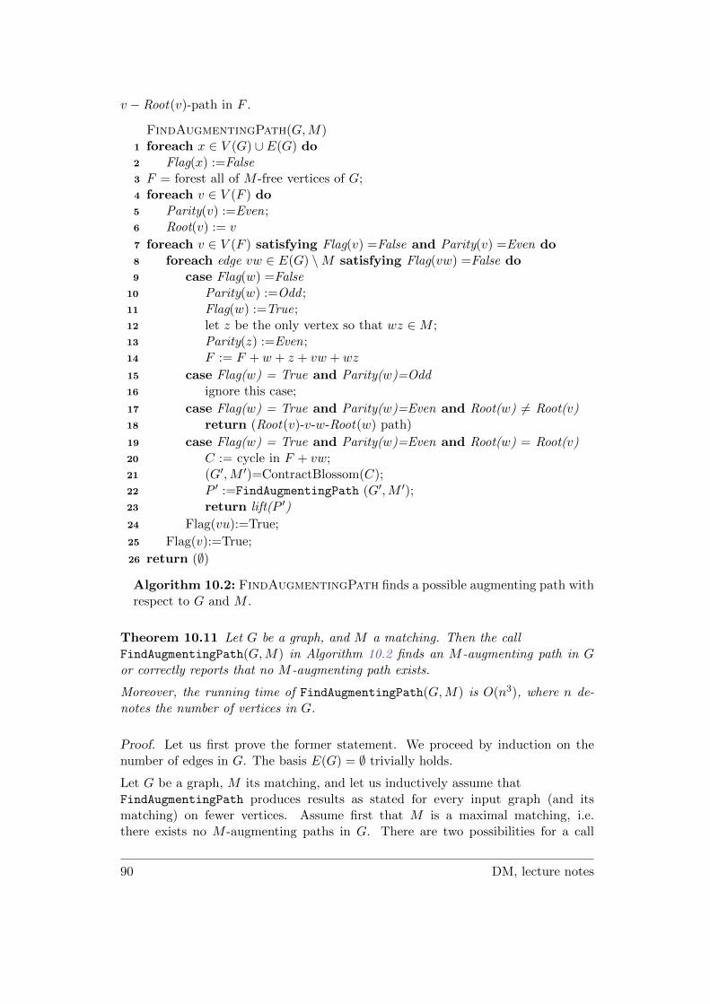
v − Root(v)-path in F .

FindAugmentingPath(G,M)1 foreach x ∈ V (G) ∪ E(G) do2 Flag(x) :=False3 F = forest all of M -free vertices of G;4 foreach v ∈ V (F ) do5 Parity(v) :=Even;6 Root(v) := v

7 foreach v ∈ V (F ) satisfying Flag(v) =False and Parity(v) =Even do8 foreach edge vw ∈ E(G) \M satisfying Flag(vw) =False do9 case Flag(w) =False

10 Parity(w) :=Odd ;11 Flag(w) :=True;12 let z be the only vertex so that wz ∈M ;13 Parity(z) :=Even;14 F := F + w + z + vw + wz

15 case Flag(w) = True and Parity(w)=Odd16 ignore this case;

17 case Flag(w) = True and Parity(w)=Even and Root(w) 6= Root(v)18 return (Root(v)-v-w-Root(w) path)

19 case Flag(w) = True and Parity(w)=Even and Root(w) = Root(v)20 C := cycle in F + vw;21 (G′,M ′)=ContractBlossom(C);22 P ′ :=FindAugmentingPath (G′,M ′);23 return lift(P ′)

24 Flag(vu):=True;

25 Flag(v):=True;

26 return (∅)

Algorithm 10.2: FindAugmentingPath finds a possible augmenting path withrespect to G and M .

Theorem 10.11 Let G be a graph, and M a matching. Then the callFindAugmentingPath(G,M) in Algorithm 10.2 finds an M -augmenting path in Gor correctly reports that no M -augmenting path exists.

Moreover, the running time of FindAugmentingPath(G,M) is O(n3), where n de-notes the number of vertices in G.

Proof. Let us first prove the former statement. We proceed by induction on thenumber of edges in G. The basis E(G) = ∅ trivially holds.

Let G be a graph, M its matching, and let us inductively assume thatFindAugmentingPath produces results as stated for every input graph (and itsmatching) on fewer vertices. Assume first that M is a maximal matching, i.e.there exists no M -augmenting paths in G. There are two possibilities for a call


FindAugmentingPath(G,M) to return a path. Either the algorithm outputs ∅ (anindication that there exists no M -augmenting path) on Line 26 or outputs a lift(P ′)on Line 23, where P ′ is a path returned by the call FindAugmentingPath(G′,M ′).As the contracted graph G′ contains no M ′-augmenting path by Theorem 10.10, theinductive hypothesis implies P ′ = ∅. Hence also lift(P ′) = ∅.Assume next that there exists an M -augmenting path P = v0v1v2 . . . vk in G. In or-der to achieve a contradiction let us assume that the call FindAugmentingPath(G,M)returns ∅. Inductively we may assume that the primary routineFindAugmentingPath(G,M) does not recursively call FindAugmentingPath(G′,M ′),and finishes by returning ∅ on line 26. This implies that every vertex v having evenparity is ultimately flagged.

Let us inductively prove that for every vertex vi of P its parity equals the parity of i.This clearly is true for i = 0. Now consider an edge vivi+1 of P . If vivi+1 6∈M then viand vi+1 have different parities, as inductively vi is of even parity and as otherwiseFindAugmentingPath(G,M) returns an augmenting path or finds a blossom. Ifvivi+1 ∈M then we may by induction assume that vi is of odd parity. Now if parityof vi was set before vi+1 then vi+1 is the only neighbor of vi along an edge in Mand immediately after Line 12 the parity of vi+1 is set to even. On the other handif parity of vi+1 is odd then at the moment the parity of vi+1 was set the vertexvi had not been determined its parity. That would make vi of even parity whichcontradicts the inductive assumption.

Hence vi and i are of the same parity along all P . This is clearly a contradiction ask is odd, and as vk is M -free, its parity is even.

For the time complexity it is easy to see that a single call ofFindAugmentingPath(G,M), excluding recursion, takes O(m) = O(n2) time, wherem denotes the number of edges in G. As G′ contains fewer edges, the total timecomplexity of FindAugmentingPath(G,M) including the recursive calls is boundedabove by O(

∑ni=1 i

2) = O(n3). �

Now let us finish with a couple of comments. Using the template Algorithm 10.1 weinfer that we can compute maximal matchings in general graphs in time O(n4).

If the input graph G is bipartite then the case on line 19 never occurs. This impliesthat FindAugmentingPath can be used also for computing maximal matchings inbipartite graph. A single call of FindAugmentingPath takes O(m) which impliesthat we can compute maximal matchings in bipartite graphs in time O(nm).

Finally let us argue that looking for blossoms in indeed necessary. If M is not amaximal matching in G, then G contains an M -augmenting path, but we may notfind it with the search approach employed in Algorithm 10.2. The catch lies in caseon line 15. An edge vw is in this case ignored, but may itself be an edge of anM -augmenting path P , as P may use a number of not yet discovered vertices.


discrete mathematics lecture notesmatematika.fri.uni-lj.si/dm/discrete_mathematics.pdf · the...

Documents