discrete colonel blotto and general lotto games · discrete colonel blotto and general lotto games...

Int J Game Theory (2008) 36:441–460DOI 10.1007/s00182-007-0099-9

ORIGINAL PAPER

Discrete Colonel Blotto and General Lotto games

Sergiu Hart

Accepted: 5 May 2007 / Published online: 12 October 2007© Springer-Verlag 2007

Abstract A class of integer-valued allocation games—“General Lotto games”—isintroduced and solved. The results are then applied to analyze the classical discrete“Colonel Blotto games”; in particular, optimal strategies are obtained for all symmetricColonel Blotto games.

1 Introduction

There are two players, Player A and Player B. Player A is given A alabaster marblesto distribute any way he wants into K urns, and Player B is given B black marbles to(simultaneously) distribute into the same K urns. One urn is chosen at random (eachurn is equally likely to be chosen); if it contains more alabaster marbles than blackmarbles, A wins; if it contains more black marbles than alabaster marbles, B wins;otherwise it is a draw. This two-person zero-sum game (a win is +1, a loss is −1,

and a tie is 0), which we denote B(A, B; K ), is known in the literature as a ColonelBlotto game: each urn represents a “battlefield,” and the number of marbles in urni corresponds to the number of “battalions” sent to battlefield i ; see Borel (1921),Tukey (1949), Shubik (1982). This class of games is a prime example of “allocation”

Dedicated with great admiration to David Gale on his 85th birthday.

Research partially supported by a grant of the Israel Science Foundation. The author thanks JudithAvrahami and Yaakov Kareev for raising the problem, Abraham Neyman for useful suggestions,and Tom Ferguson, Benny Moldovanu, and Aner Sela for comments and discussions.

S. Hart (B)Center for the Study of Rationality, Institute of Mathematics and Department of Economics,The Hebrew University of Jerusalem, Jerusalem, Israele-mail: [email protected]: http://www.ma.huji.ac.il/hart

123

442 S. Hart

games, where sides compete on different “fronts” and need to allocate their resourcesoptimally among them. Some examples are lobbying and campaigning by politicalparties, research and development competitions among firms, and multi-unit and all-pay auctions.

How should the game be played? For example, when A = 24, B = 18, and K = 8?The problem turns out to be quite difficult, in part due to the integer restriction on thenumber of balls in each urn. Most of the literature has relaxed this condition; seeRobertson (2006) for a complete solution of the “continuous” version and a survey ofthe literature.

Here we will proceed along a different route, one that respects the integer constraint.Specifically, we consider in Sect. 2 a variant of Colonel Blotto games—the “GeneralLotto games”—which we solve in Sect. 3: we find the value and optimal strategies.In Sect. 4 we show that certain optimal strategies of General Lotto games can beimplemented in Colonel Blotto games. This yields, in particular, optimal strategies forall symmetric Colonel Blotto games (i.e., when A = B), as well as for other cases.We conclude with a discussion in Sect. 5.

2 Lotto Games

We consider two variants of the Colonel Blotto games, which we call “Colonel Lottogames” and “General Lotto games.”

2.1 Colonel Lotto Games

Assume that the K urns are indistinguishable. This is easily seen to be equivalent tothe following. Player A has K alabaster urns of his own, Player B has K black urns ofhis own, and, after each player distributes his marbles into his own urns, one alabasterurn and one black urn are chosen at random (all urns have the same probability of beingchosen), and the contents of the two urns are compared to determine the winner.1 Thisis a “symmetrized-across-urns” version of the Colonel Blotto game; we will refer toit as a Colonel Lotto game, and denote it L(A, B; K ).

In both games a pure strategy of Player A is a K-partition x = 〈 x1, x2, . . . , xK 〉of A, i.e., nonnegative integers x1, x2, . . . , xK with x1 + x2 + · · · + xK = A, and apure strategy of Player B is a K-partition y = 〈 y1, y2, . . . , yK 〉 of B. The payoff inthe Colonel Blotto game is2

hB(x, y) = 1

K

K∑

k=1

sign (xk − yk),

1 Avrahami and Kareev (2005) have conducted a laboratory experiment on this specific version of thegame.2 sign (z) = 1 when z > 0; sign (z) = −1 when z < 0; and sign (0) = 0.

123

Discrete Colonel Blotto and General Lotto games 443

whereas in the Colonel Lotto game it is

hL(x, y) = 1

K 2

K∑

k=1

K∑

�=1

sign (xk − y�).

For a pure strategy x of Player A, let σ(x)be the mixed strategy that gives probability1/K ! to each one of the K ! permutations of x; then3 hB(σ (x), y) = hL(x, y) for allpure strategies y of Player B. For a mixed strategy ξ of Player A, let σ(ξ) be the mixedstrategy obtained by replacing each pure x in the support of ξ by its corresponding4

σ(x); then hB(σ (ξ), y) = hL(ξ, y) for all pure y, and so hB(σ (ξ), η) = hL(ξ, η)

for all mixed strategies η of Player B (we will refer to the strategies σ(x) and σ(ξ) assymmetric across urns). The same holds for Player B, and we thus have:

The Colonel Blotto game B(A, B; K ) and the Colonel Lotto game L(A, B; K )

have the same value. Moreover, the mapping σ maps the optimal strategies in theColonel Lotto game onto the optimal strategies in the Colonel Blotto game that aresymmetric across urns.5

2.2 General Lotto Games

Let x = 〈 x1, x2, . . . , xK 〉 be a pure strategy of Player A, i.e., a K-partition of A. Wewill view x as a random variable X whose values are x1, x2, . . . , xK with probability1/K each. For example, x = 〈 0, 0, 0, 0, 5, 5, 5, 9 〉 (for A = 24 and K = 8) yieldsP(X = 0) = 4/8 = 1/2, P(X = 5) = 3/8, and P(X = 9) = 1/8; we willwrite this as6 X = (1/2)10 + (3/8)15 + (1/8)19. The expectation of X is E(X) =(1/K )

∑Ki=1 xi = A/K , which is the average number of marbles per urn. Similarly,

let the random variable Y correspond to the strategy y = 〈 y1, y2, . . . , yK 〉 of PlayerB; then the (expected) payoff hL(x, y) in the Colonel Lotto game equals

H(X, Y ) := P(X > Y ) − P(X < Y ). (1)

We now consider the generalization where X and Y are allowed to be any non-negative integer-valued random variables with expectations E(X) = A/K = a andE(Y ) = B/K = b, respectively. That is, we remove the restriction that they can bederived from probability distributions on K-partitions.

For each a, b > 0 we thus define the game �(a, b) where Player A chooses a(distribution of a) nonnegative integer-valued random variable X with expectationE(X) = a, and Player B chooses a (distribution of a) nonnegative integer-valued

3 We will write h also for the (bilinear) extension of the payoff function to pairs of mixed strategies.4 Equivalently, choose a random numbering of the K urns and use ξ.

5 However, there may be optimal strategies in Colonel Blotto games that are not symmetric across urns.6 1i denotes the Dirac measure which puts probability one on i . For simplicity, we will identify a randomvariable with its distribution.

123

444 S. Hart

random variable Y with E(Y ) = b, and the payoff is given by (1) with X and Y takento be independent.7 We will call �(a, b) a General Lotto game.

In Sect. 3 we will prove that each General Lotto game has a minimax value; we doso by providing explicit optimal strategies for both players (see Fig. 1 for a summary).8

2.3 Continuous General Lotto Games

Before proceeding to the analysis of the General Lotto games, it is instructive to presenta further generalization, which dispenses also with the integer-valued restriction. Ina Continuous General Lotto game, which we denote �(a, b), Player A chooses a(distribution of a) nonnegative random variable X with E(X) = a, Player B choosesa (distribution of a) nonnegative random variable Y with E(Y ) = b, and the payoff isgiven by H(X, Y ) as defined in (1) with X and Y independent.

Theorem 1 Let a ≥ b > 0. The value of the Continuous General Lotto game �(a, b)

is

val �(a, b) = a − b

a= 1 − b

a,

and the unique optimal strategies are X∗ = U (0, 2a) for Player A and Y ∗ =(1 − b/a)10 + (b/a)U (0, 2a) for Player B.9

When a > b the strategies of Theorem 1 can be interpreted as follows. The strongerPlayer A plays a uniform distribution with expectation a, on the interval (0, 2a). Theweaker Player B “gives up” and plays 0 with probability 1 − b/a, and with theremaining probability b/a he “matches” the stronger player (by playing the sameuniform distribution on (0, 2a)); the probability b/a is chosen so that the expectationwill indeed be b. The special case where the game is symmetric, i.e., a = b, hasbeen solved by Bell and Cover (1980, Sect. 2); see also Myerson (1993) and Lizzeri(1999). The solution of the nonsymmetric case (a > b) is due to Sahuguet and Persico(2006). In the Appendix we will provide an elementary direct proof (the difficultylies in showing the uniqueness of the optimal strategies; Sahuguet and Persico use areduction to “all-pay auction” games and apply known results there, which makes theproof quite complex).

7 Equivalently, let the payoff be sign(X − Y ) where X and Y are two independent draws from the twochosen distributions.8 Since the game �(a, b) has infinitely many pure strategies, the classical Minimax Theorem for finitegames does not apply to it. However, the existence of value can be shown also by finite-approximationarguments (as pointed out by Abraham Neyman). Finally, as the set of distributions of nonnegative integer-valued random variables X with a given expectation is already convex (and the payoff is linear in thedistribution of X), no further mixtures are needed.9 Throughout this paper we identify a random variable with its distribution; thus Y = λ10 + (1 − λ)Umeans that Y = 0 with probability λ and Y = U with probability 1−λ. The notation U (c, d) stands for theuniform distribution on the interval (c, d); the cumulative distribution functions are thus FX∗ (x) = x/(2a)

for all x ∈ [0, 2a], and FY ∗ (y) = by/(2a2) for all y ∈ (0, 2a] and FY ∗ (0) = 1 − b/a.

123


3 Solution of the General Lotto Games

In this section we will solve the General Lotto games. We will assume throughout thatall random variables are nonnegative and integer-valued. Every such random variableX is

∑∞i=0 pi 1i where pi = P(X = i) (so pi ≥ 0 for all i and

∑i pi = 1). Also,

E(X) = ∑∞i=1 i P(X = i) = ∑∞

i=1 P(X ≥ i). For every Y we have

H(X, Y ) =∞∑

i=0

pi [P(i > Y ) − P(i < Y )]

=∞∑

i=0

pi [1 − P(Y ≥ i) − P(Y ≥ i + 1)]

= 1 −∞∑

i=0

pi [P(Y ≥ i) + P(Y ≥ i + 1)] .

For every positive integer m we define three uniform distributions, each one withexpectation m:

U m := U ({0, 1, . . . , 2m}) =2m∑

i=0

(1

2m + 1

)1i ;

U mo := U ({1, 3, . . . , 2m − 1}) =

m∑

i=1

(1

m

)12i−1; and

U me := U ({0, 2, . . . , 2m}) =

m∑

i=0

(1

m + 1

)12i

(think of U mo and U m

e as “uniform on odd numbers” and “uniform on even numbers,”respectively; note that U m is the average of U m

o and U me , with weights m/(2m + 1)

and (m + 1)/(2m + 1), respectively). For every Y we get

H(U mo , Y ) = 1 − 1

m

m∑

i=1

[P(Y ≥ 2i − 1) + P(Y ≥ 2i)]

= 1 − 1

m

2m∑

j=1

P(Y ≥ j) ≥ 1 − E(Y )

m, (2)

with equality if and only if∑∞

j=2m+1 P(Y ≥ j) = 0, or Y ≤ 2m; and

H(U me , Y ) = 1 − 1

m + 1

m∑

i=0

[P(Y ≥ 2i) + P(Y ≥ 2i + 1)]

123

446 S. Hart

= 1 − 1

m + 1

⎛

⎝2m+1∑

j=1

P(Y ≥ j) + P(Y ≥ 0)

⎞

⎠

≥ 1 − E(Y ) + 1

m + 1, (3)

with equality if and only if∑∞

j=2m+2 P(Y ≥ j) = 0, or Y ≤ 2m + 1.

Let a ≥ b > 0; we will distinguish three cases in the analysis of �(a, b):

• a is an integer (Theorem 2);• a is not an integer and10 �a < b� (Theorem 3); and• a is not an integer and �a ≥ b� (Theorem 4).

See the table of Fig. 1 at the end of this section for a summary of the results. As inthe Continuous General Lotto games, the main difficulties lie in characterizing theoptimal strategies.

Theorem 2 Let a ≥ b > 0 where a is an integer. Then the value of the General Lottogame �(a, b) is

val �(a, b) = a − b

a= 1 − b

a.

The optimal strategies are as follows:

(i) When a = b the strategy X is optimal (for either player) if and only if11

X ∈ conv{U ao , U a

e }.(ii) When a > b the strategy U a

o is the unique optimal strategy of Player A.

(iii) When a > b the strategies (1 − b/a)10 + (b/a)V with V ∈ conv{U ao , U a

e } areoptimal strategies of Player B.

(iv) Every optimal strategy Y of Player B satisfies Y ≤ 2a and

1 − b

a≤ P(Y = 0) ≤ 1 − b

a + 1.

Proof Using (2), (3), and H(X, Y ) = −H(Y, X) we get the following: in the game�(a, a) (i.e., when a = b), for all X and Y with E(X) = E(Y ) = a,

H(U ar , Y ) ≥ 0 ≥ H(X, U a

s ) (4)

for r, s ∈ {o,e}. In the game �(a, b) with a > b, for all X with E(X) = a and Y withE(Y ) = b we get

H(U ao , Y ) ≥ 1 − b

a≥ H

(X, Y a,b

r

)(5)

10 �z is the largest integer ≤ z, and z� is the smallest integer ≥ z.11 conv{U1, U2} denotes the convex hull of U1 and U2, i.e., the set of λU1 + (1 − λ)U2 for all λ ∈ [0, 1].

123


for r ∈ {o,e}, where Y a,br = (1 − b/a)10 + (b/a)U a

r , with the second inequalityobtained as follows:

H(

X, Y a,br

)=

(1 − b

a

)P(X > 0) +

(b

a

)H(X, U a

r )

=(

1 − b

a

)P(X > 0) −

(b

a

)H(U a

r , X)

≤(

1 − b

a

)1 −

(b

a

)0 = 1 − b

a. (6)

This proves that the value of �(a, b) is 1 − b/a, and that all the strategies above areoptimal (and so are their convex combinations).

To prove (i), let X0 be an optimal strategy12 in �(a, a), i.e., H(X0, Y ) ≥ 0 for allY with E(Y ) = a; therefore H(X0, U a

r ) = 0 for r ∈ {o,e} (since the U ar are optimal),

which implies equality in (2), and so X0 ≤ 2a.

For every i, j with 0 ≤ i ≤ a ≤ j ≤ 2a, let Ti, j ≡ T ai, j be the distribution

λ1i + (1 − λ)1 j with expectation a, i.e., λ = ( j − a)/( j − i) (when i = a or j = athis is just 1a). The distribution U a gives positive probability to both i and j, so wecan express it as U a = τT a

i, j + (1 − τ)W for some 0 < τ < 1 and W ≥ 0 withE(W ) = a (indeed, take τ > 0 so that both τλ and τ(1 − λ) are ≤ 1/(2a + 1)). NowH(X0, T a

i, j ) ≥ 0 and H(X0, W ) ≥ 0 (since T ai, j and W each have expectation a) and

H(X0, U a) = 0 (since U a is optimal), so we must have equality: H(X0, T ai, j ) = 0.

Therefore λH(X0, 1i ) + (1 − λ)H(X0, 1 j ) = 0, or, denoting wi := H(X0, 1i )

( j − a)wi + (a − i)w j = 0 (7)

for every 0 ≤ i ≤ a ≤ j ≤ 2a. Taking i = a − 1 gives w j = −( j − a)wa−1 =(a − j)wa−1 for all j ≥ a, in particular wa+1 = −wa−1; taking j = a + 1 giveswi = −(a − i)wa+1 = (a − i)wa−1 for every i ≤ a, so wi = (a − i)wa−1 holds forall 0 ≤ i ≤ 2a. Therefore

wi − wi+1 = wa−1 for all 0 ≤ i ≤ 2a − 1. (8)

Let qi :=P(X0 = i); then wi −wi+1 =(P(X0 > i)−P(X0 < i)

)−(P(X0 > i + 1)−

P(X0 < i + 1)) = qi + qi+1, so (8) implies qi + qi+1 = qi+1 + qi+2, or qi =

qi+2, for all 0 ≤ i ≤ 2a − 2. Therefore X0 = ∑ai=0 q012i + ∑a

i=1 q112i−1 =((a + 1)q0)U a

e + (aq1)U ao , or X0 ∈ conv{U a

o , U ae }, which completes the proof of (i).

To prove (ii), let X0 be optimal for Player A in �(a, b) when a > b. Equality in(6) for X = X0 implies P(X > 0) = 1 and X0 ≤ 2a (recall (2)), or 1 ≤ X0 ≤ 2a.

Therefore, for every Y with E(Y ) = a we have 1 − b/a ≤ H(X0, (1 − b/a)10 +(b/a)Y ) = (1 − b/a) + (b/a)H(X0, Y ); hence H(X0, Y ) ≥ 0. So X0 is an optimalstrategy in �(a, a), and therefore X0 ∈ conv{U a

o , U ae} by (i). But P(U a

e = 0) > 0whereas P(X0 = 0) = 0, so X0 = U a

o , which completes the proof of (ii).

12 For either player, since the game �(a, a) is symmetric.

123

448 S. Hart

(iii) we have already seen in (6). To prove (iv), let Y 0 be an optimal strategy of PlayerB in�(a, b).We must have equality in (2), so Y 0≤2a.Let X = U ({2, 4, . . . , 2a−2}) =∑a−1

i=1 (1/(a − 1))12i ; then E(X) = a and

1 − b

a≥ H(X, Y 0) = 1 − 1

a − 1

a−1∑

i=1

[P(Y 0 ≥ 2i) + P(Y 0 ≥ 2i + 1)

]

= 1 − 1

a − 1

2a−1∑

j=2

P(Y 0 ≥ j) ≥ 1 − 1

a − 1

(E(Y 0) − P(Y 0 ≥ 1)

)

= 1 − 1

a − 1

(b − 1 + P(Y 0 = 0)

),

from which it follows that P(Y 0 = 0) ≥ 1 − b/a.

Next, H(T a1,2a−1, Y 0) = 1 − b/a (since, as in the proof of (i) above, the optimal

strategy U ao of Player A can be expressed as τT1,2a−1 + (1−τ)W for some 0 < τ < 1

and W with E(W ) = a). Denoting qi := P(Y 0 = i), we have

1

2(2q0 + q1 − 1) + 1

2(1 − 2q2a − q2a−1) = 1 − b

a.

Also, H(T a1,2a, Y 0) ≤ 1 − b/a, i.e.,

a

2a − 1(2q0 + q1 − 1) + a − 1

2a − 1(1 − q2a) ≤ 1 − b

a.

Multiplying this inequality by (2a − 1)/(a − 1) and subtracting the previous equationfrom it yields

a + 1

a − 1q0 + a + 1

2(a − 1)q1 + 1

2q2a−1 − 1

a − 1≤ a

a − 1

(1 − b

a

);

hence P(Y 0 = 0) = q0 ≤ 1 − b/(a + 1) (we have used q1, q2a−1 ≥ 0), whichcompletes the proof of (iv). �

When a > b Player B may have additional optimal strategies beyond those in(iii); for example, when a = 4 and b = 1 (the value of �(4, 1) is 3/4), the strategyY 0 = (25/32)10 +(1/16)12 +(1/32)14 +(1/16)15 +(1/16)17, which is not a convexcombination of (3/4)10 +(1/4)U 4

o and (3/4)10 +(1/4)U 4e , is nevertheless optimal.13

We now come to the second case, where a is not an integer and �a < b� .

13 Let X = ∑i pi 1i with E(X) = 4 be a best reply to Y ∗; then X ≤ 8, and a straightforward computation

shows that H(X, Y ∗)−3/4 = H(X, Y ∗)−(1/2)∑

i pi −(1/16)∑

i i pi = −(23/32)p0 −(1/32)p4 ≤ 0.

123


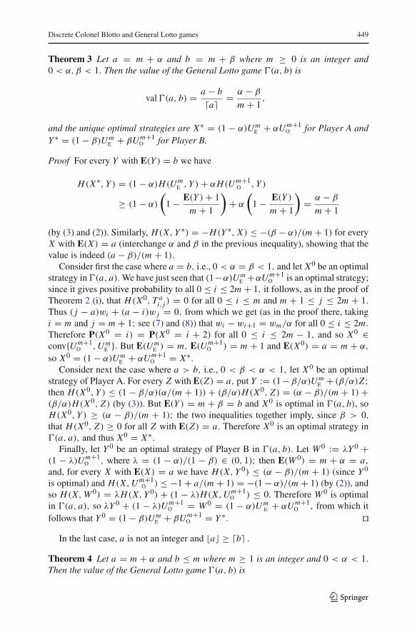
Theorem 3 Let a = m + α and b = m + β where m ≥ 0 is an integer and0 < α, β < 1. Then the value of the General Lotto game �(a, b) is

val �(a, b) = a − b

a� = α − β

m + 1,

and the unique optimal strategies are X∗ = (1 − α)U me + αU m+1

o for Player A andY ∗ = (1 − β)U m

e + βU m+1o for Player B.

Proof For every Y with E(Y ) = b we have

H(X∗, Y ) = (1 − α)H(U me , Y ) + αH(U m+1

o , Y )

≥ (1 − α)

(1 − E(Y ) + 1

m + 1

)+ α

(1 − E(Y )

m + 1

)= α − β

m + 1

(by (3) and (2)). Similarly, H(X, Y ∗) = −H(Y ∗, X) ≤ −(β − α)/(m + 1) for everyX with E(X) = a (interchange α and β in the previous inequality), showing that thevalue is indeed (a − β)/(m + 1).

Consider first the case where a = b, i.e., 0 < α = β < 1, and let X0 be an optimalstrategy in �(a, a). We have just seen that (1−α)U m

e +αU m+1o is an optimal strategy;

since it gives positive probability to all 0 ≤ i ≤ 2m + 1, it follows, as in the proof ofTheorem 2 (i), that H(X0, T a

i, j ) = 0 for all 0 ≤ i ≤ m and m + 1 ≤ j ≤ 2m + 1.

Thus ( j − a)wi + (a − i)w j = 0, from which we get (as in the proof there, takingi = m and j = m + 1; see (7) and (8)) that wi − wi+1 = wm/α for all 0 ≤ i ≤ 2m.

Therefore P(X0 = i) = P(X0 = i + 2) for all 0 ≤ i ≤ 2m − 1, and so X0 ∈conv{U m+1

o , U me }. But E(U m

e ) = m, E(U m+1o ) = m + 1 and E(X0) = a = m + α,

so X0 = (1 − α)U me + αU m+1

o = X∗.Consider next the case where a > b, i.e., 0 < β < α < 1, let X0 be an optimal

strategy of Player A. For every Z with E(Z) = a, put Y := (1 −β/α)U me + (β/α)Z;

then H(X0, Y ) ≤ (1 − β/α)(α/(m + 1)) + (β/α)H(X0, Z) = (α − β)/(m + 1) +(β/α)H(X0, Z) (by (3)). But E(Y ) = m + β = b and X0 is optimal in �(a, b), soH(X0, Y ) ≥ (α − β)/(m + 1); the two inequalities together imply, since β > 0,that H(X0, Z) ≥ 0 for all Z with E(Z) = a. Therefore X0 is an optimal strategy in�(a, a), and thus X0 = X∗.

Finally, let Y 0 be an optimal strategy of Player B in �(a, b). Let W 0 := λY 0 +(1 − λ)U m+1

o , where λ = (1 − α)/(1 − β) ∈ (0, 1); then E(W 0) = m + α = a,

and, for every X with E(X) = a we have H(X, Y 0) ≤ (α − β)/(m + 1) (since Y 0

is optimal) and H(X, U m+1o ) ≤ −1 + a/(m + 1) = −(1 − α)/(m + 1) (by (2)), and

so H(X, W 0) = λH(X, Y 0) + (1 − λ)H(X, U m+1o ) ≤ 0. Therefore W 0 is optimal

in �(a, a), so λY 0 + (1 − λ)U m+1o = W 0 = (1 − α)U m

e + αU m+1o , from which it

follows that Y 0 = (1 − β)U me + βU m+1

o = Y ∗. �In the last case, a is not an integer and �a ≥ b� .

Theorem 4 Let a = m + α and b ≤ m where m ≥ 1 is an integer and 0 < α < 1.

Then the value of the General Lotto game �(a, b) is

123

450 S. Hart

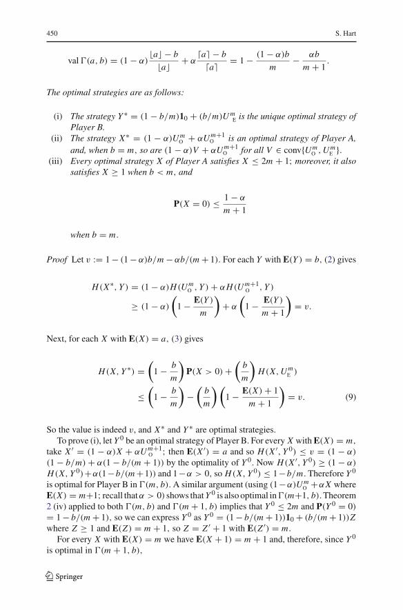
val �(a, b) = (1 − α)�a − b

�a + αa� − b

a� = 1 − (1 − α)b

m− αb

m + 1.

The optimal strategies are as follows:

(i) The strategy Y ∗ = (1 − b/m)10 + (b/m)U me is the unique optimal strategy of

Player B.(ii) The strategy X∗ = (1 − α)U m

o + αU m+1o is an optimal strategy of Player A,

and, when b = m, so are (1 − α)V + αU m+1o for all V ∈ conv{U m

o , U me }.

(iii) Every optimal strategy X of Player A satisfies X ≤ 2m + 1; moreover, it alsosatisfies X ≥ 1 when b < m, and

P(X = 0) ≤ 1 − α

m + 1

when b = m.

Proof Let v := 1 − (1 − α)b/m − αb/(m + 1). For each Y with E(Y ) = b, (2) gives

H(X∗, Y ) = (1 − α)H(U mo , Y ) + αH(U m+1

o , Y )

≥ (1 − α)

(1 − E(Y )

m

)+ α

(1 − E(Y )

m + 1

)= v.

Next, for each X with E(X) = a, (3) gives

H(X, Y ∗) =(

1 − b

m

)P(X > 0) +

(b

m

)H(X, U m

e )

≤(

1 − b

m

)−

(b

m

) (1 − E(X) + 1

m + 1

)= v. (9)

So the value is indeed v, and X∗ and Y ∗ are optimal strategies.To prove (i), let Y 0 be an optimal strategy of Player B. For every X with E(X) = m,

take X ′ = (1 − α)X + αU m+1o ; then E(X ′) = a and so H(X ′, Y 0) ≤ v = (1 − α)

(1 − b/m) + α(1 − b/(m + 1)) by the optimality of Y 0. Now H(X ′, Y 0) ≥ (1 − α)

H(X, Y 0)+α(1−b/(m +1)) and 1−α > 0, so H(X, Y 0) ≤ 1−b/m. Therefore Y 0

is optimal for Player B in �(m, b). A similar argument (using (1−α)U mo +αX where

E(X) = m+1; recall thatα > 0) shows that Y 0 is also optimal in�(m+1, b).Theorem2 (iv) applied to both �(m, b) and �(m + 1, b) implies that Y 0 ≤ 2m and P(Y 0 = 0)

= 1 − b/(m + 1), so we can express Y 0 as Y 0 = (1 − b/(m + 1))10 + (b/(m + 1))Zwhere Z ≥ 1 and E(Z) = m + 1, so Z = Z ′ + 1 with E(Z ′) = m.

For every X with E(X) = m we have E(X + 1) = m + 1 and, therefore, since Y 0

is optimal in �(m + 1, b),

123


1 − b

m + 1≥ H(X + 1, Y 0)

=(

1 − b

m + 1

)P(X + 1 > 0) +

(b

m + 1

)H(X + 1, Z ′ + 1)

= 1 − b

m + 1+

(b

m + 1

)H(X, Z ′);

hence14 H(X, Z ′) ≤ 0. Therefore Z ′ is optimal in �(m, m), which implies byTheorem 2 (i) that Z ′ ∈ conv{U m

o , U me }. We have seen above that Y 0 ≤ 2m, so

Z ≤ 2m and Z ′ ≤ 2m − 1, which implies that in fact Z ′ = U mo (since U m

e , andthus all other elements of conv{U m

o , U me }, give positive probability to 2m). Hence

Y 0 = (1 − b/(m + 1))10 + (b/(m + 1))(U mo + 1) = (1 − b/m)10 + (b/m)U m

e = Y ∗,which proves (i).

To prove (ii): We have already seen that X∗ is an optimal strategy of Player A.When b = m, for every Y with E(Y ) = m we have H((1 − α)U m

r + αU m+1o , Y ) =

(1−α) 0+α(1/(m+1)) = 1−(1−α)(m/m)−α(m/(m+1)), so (1−α)U mr +αU m+1

ois indeed optimal for Player A in �(m + α, m).

Finally, to show (iii), let X0 be an optimal strategy of Player A. Equality in (9)implies that it must satisfy X0 ≤ 2m + 1 (recall (3)) and, when b < m, also P(X0 >

0) = 1. When b = m, take Y = (1/(m +1))10 + (m/(m +1))U m+1o ; then E(Y ) = m

and

α

m + 1= val �(m + α, m) ≤ H(X0, Y )

= 1

m + 1P(X0 > 0) + m

m + 1H(X0, U m+1

o )

≤ 1

m + 1(1 − P(X0 = 0)) − m

m + 1

(1 − m + α

m + 1

)

(recall (2)), which yields P(X0 = 0) ≤ (1 − α)/(m + 1). �Again, there are additional optimal strategies for Player A; for example, X =

(1/2)11 + (1/2)12 is optimal in �(3/2, 1) and X = (5/12)11 + (1/4)13 + (1/3)14 isoptimal in �(5/2, 1/2).

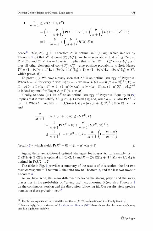
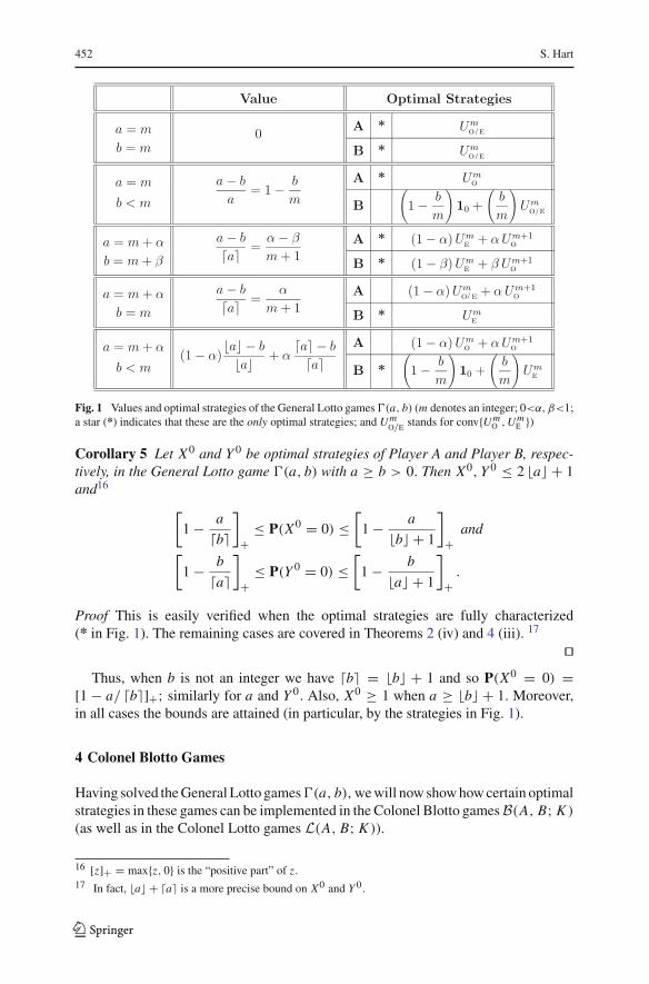
The table in Fig. 1 provides a summary of the results of this section: the first tworows correspond to Theorem 2, the third row to Theorem 3, and the last two rows toTheorem 4.

As we have seen, the main difference between the strong player and the weakplayer lies in the probability of “giving up,” i.e., choosing 0 (see also Theorem 1on the continuous version and the discussion following it). Our results yield precisebounds on these probabilities.15

14 For the last equality we have used the fact that H(X, Y ) is a function of X − Y only (see (1)).15 Interestingly, the experiments of Avrahami and Kareev (2005) have shown that the number of emptyurns is a significant variable.

123

452 S. Hart

Fig. 1 Values and optimal strategies of the General Lotto games �(a, b) (m denotes an integer; 0<α, β<1;a star (*) indicates that these are the only optimal strategies; and Um

o/e stands for conv{Umo , Um

e })

Corollary 5 Let X0 and Y 0 be optimal strategies of Player A and Player B, respec-tively, in the General Lotto game �(a, b) with a ≥ b > 0. Then X0, Y 0 ≤ 2 �a + 1and16

[1 − a

b�]

+≤ P(X0 = 0) ≤

[1 − a

�b + 1

]

+and

[1 − b

a�]

+≤ P(Y 0 = 0) ≤

[1 − b

�a + 1

]

+.

Proof This is easily verified when the optimal strategies are fully characterized(* in Fig. 1). The remaining cases are covered in Theorems 2 (iv) and 4 (iii). 17

�Thus, when b is not an integer we have b� = �b + 1 and so P(X0 = 0) =

[1 − a/ b�]+; similarly for a and Y 0. Also, X0 ≥ 1 when a ≥ �b + 1. Moreover,in all cases the bounds are attained (in particular, by the strategies in Fig. 1).

4 Colonel Blotto Games

Having solved the General Lotto games �(a, b), we will now show how certain optimalstrategies in these games can be implemented in the Colonel Blotto games B(A, B; K )

(as well as in the Colonel Lotto games L(A, B; K )).

16 [z]+ = max{z, 0} is the “positive part” of z.17 In fact, �a + a� is a more precise bound on X0 and Y 0.

123


Let A ≥ 1 and K ≥ 2 be integers. Recall (Sect. 2.2 ) that we identify aK-partition x = 〈 x1, x2, . . . , xK 〉of A (i.e., x1+x2+· · ·+xK = A,where the xk are Knonnegative integers) with the distribution it generates, X = ∑K

k=1(1/K )1xk ;note thatE(X) = A/K . A nonnegative integer-valued random variable Z will be called (A, K )-feasible if Z can be obtained from a probability distribution onK-partitions of A. That is, Z is a mixed strategy of Player A in the Colonel Blottogame B(A, B; K ). Formally, it means that Z = ∑n

i=1 λi Xi , where each Xi is (thedistribution of) a K-partition of A, each λi > 0, and

∑ni=1 λi = 1. For example,

let Z = U 3e = (1/4)10 + (1/4)12 + (1/4)14 + (1/4)16; then Z is (6, 2)-feasible:

put mass 1/2 on the partition 〈 0, 6 〉 and 1/2 on the partition 〈 2, 4 〉 (their distribu-tions are, respectively, (1/2)10 + (1/2)16 and (1/2)12 + (1/2)14). However, Z is not(9, 3)-feasible, since the support of Z consists of even numbers only, whereas every3-partition of 9 must contain an odd number.

We have

Proposition 6 Let A ≥ 1 and K ≥ 2 be integers.

(i) If A = mK where m ≥ 1 is an integer, then U mo is (A, K )-feasible if and only

if A and K have the same parity (i.e., both are even or both are odd).(ii) If A = mK where m ≥ 1 is an integer, then U m

e is (A, K )-feasible if and onlyif A is even.

(iii) If A = mK + r where m ≥ 0 and 1 ≤ r ≤ K − 1 are integers, then

(1 − r

K

)U m

e +( r

K

)U m+1

o

is (A, K )-feasible.

When A/K = m is an integer, (i) and (ii) can be restated as follows. If K is even,both U m

o and U me are feasible; if K is odd, only one of them is feasible: U m

o when Ais odd and U m

e when A is even. As we will see immediately below, it turns out thatU m

o and U me are feasible except when this is ruled out by trivial parity considerations.

The proof of Proposition 6 provides explicit constructions of the appropriate distri-butions on partitions; a number of illustrative examples follow the Proof of Theorem 7.

Proof First, we note that the conditions of feasibility in (i) and (ii) are clearly necessary.Indeed, if A is the sum of K odd numbers then A has the same parity as K ; hence U m

o ,

whose support consists of odd numbers only, cannot be obtained from K-partitions ofA when A and K have different parity. Similarly, if U m

e , whose support consists ofeven numbers only, is (A, K )-feasible, then A is the sum of K even numbers, so itmust be even.

We will now construct for each case an appropriate � × K matrix S, such that eachrow is a K-partition of A (i.e., all the row sums equal A), and the required distributionX is obtained by assigning equal probability of 1/� to each row. We will say that inthis case S implements X (by K-partitions of A).

We first deal with (ii) and (iii); we distinguish two cases, according to the parityof K .

123

454 S. Hart

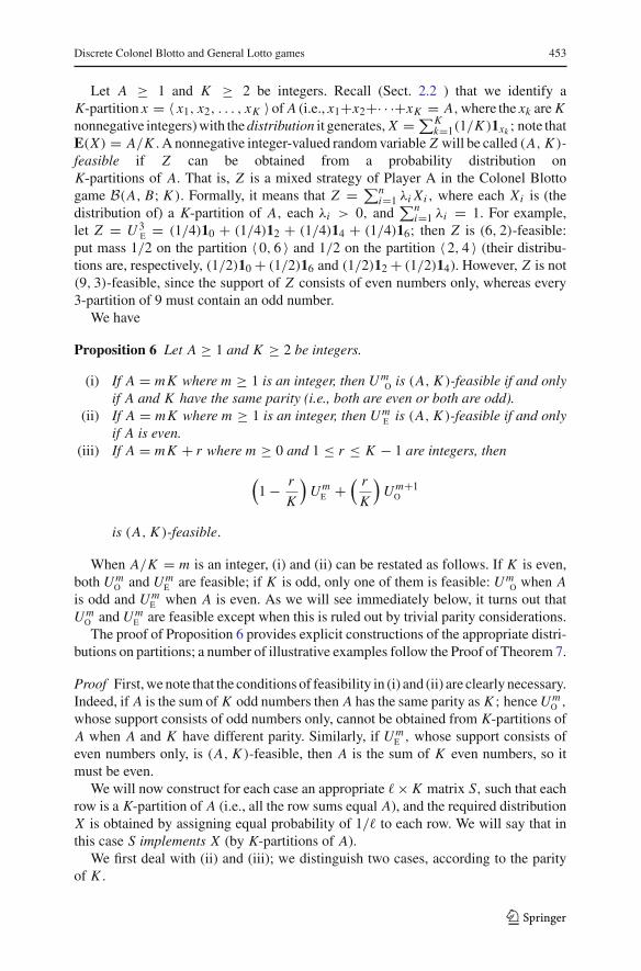
Fig. 2 The matrix S0 in Case 1

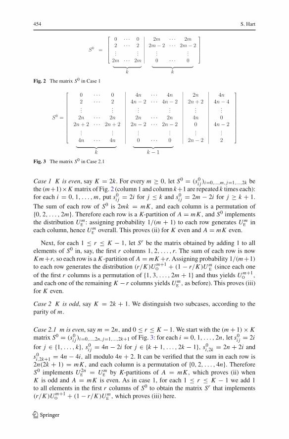
Fig. 3 The matrix S0 in Case 2.1

Case 1 K is even, say K = 2k. For every m ≥ 0, let S0 = (s0i j )i=0,...,m, j=1,...,2k be

the (m+1)×K matrix of Fig. 2 (column 1 and column k+1 are repeated k times each):for each i = 0, 1, . . . , m, put s0

i j = 2i for j ≤ k and s0i j = 2m − 2i for j ≥ k + 1.

The sum of each row of S0 is 2mk = mK , and each column is a permutation of{0, 2, . . . , 2m}. Therefore each row is a K-partition of A = mK , and S0 implementsthe distribution U m

e : assigning probability 1/(m + 1) to each row generates U me in

each column, hence U me overall. This proves (ii) for K even and A = mK even.

Next, for each 1 ≤ r ≤ K − 1, let Sr be the matrix obtained by adding 1 to allelements of S0 in, say, the first r columns 1, 2, . . . , r. The sum of each row is nowK m +r, so each row is a K -partition of A = mK +r. Assigning probability 1/(m +1)

to each row generates the distribution (r/K )U m+1o + (1 − r/K )U m

e (since each oneof the first r columns is a permutation of {1, 3, . . . , 2m + 1} and thus yields U m+1

o ,

and each one of the remaining K − r columns yields U me , as before). This proves (iii)

for K even.

Case 2 K is odd, say K = 2k + 1. We distinguish two subcases, according to theparity of m.

Case 2.1 m is even, say m = 2n, and 0 ≤ r ≤ K − 1. We start with the (m + 1) × Kmatrix S0 = (s0

i j )i=0,...,2n, j=1,...,2k+1 of Fig. 3: for each i = 0, 1, . . . , 2n, let s0i j = 2i

for j ∈ {1, . . . , k}, s0i j = 4n − 2i for j ∈ {k + 1, . . . , 2k − 1}, s0

i,2k = 2n + 2i and

s0i,2k+1 = 4n − 4i, all modulo 4n + 2. It can be verified that the sum in each row is

2n(2k + 1) = mK , and each column is a permutation of {0, 2, . . . , 4n}. ThereforeS0 implements U 2n

e = U me by K-partitions of A = mK , which proves (ii) when

K is odd and A = mK is even. As in case 1, for each 1 ≤ r ≤ K − 1 we add 1to all elements in the first r columns of S0 to obtain the matrix Sr that implements(r/K )U m+1

o + (1 − r/K )U me , which proves (iii) here.

123


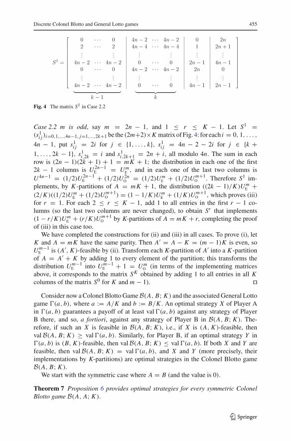
Fig. 4 The matrix S1 in Case 2.2

Case 2.2 m is odd, say m = 2n − 1, and 1 ≤ r ≤ K − 1. Let S1 =(s1

i j )i=0,1,...,4n−1, j=1,...,2k+1 be the (2m+2)×K matrix of Fig. 4: for each i = 0, 1, . . . ,

4n − 1, put s1i j = 2i for j ∈ {1, . . . , k}, s1

i j = 4n − 2 − 2i for j ∈ {k +1, . . . , 2k − 1}, s1

i,2k = i and s1i,2k+1 = 2n + i, all modulo 4n. The sum in each

row is (2n − 1)(2k + 1) + 1 = mK + 1; the distribution in each one of the first2k − 1 columns is U 2n−1

e = U me , and in each one of the last two columns is

U 4n−1 = (1/2)U 2n−1e + (1/2)U 2n

o = (1/2)U me + (1/2)U m+1

o . Therefore S1 im-plements, by K -partitions of A = mK + 1, the distribution ((2k − 1)/K )U m

e +(2/K )((1/2)U m

e + (1/2)U m+1o ) = (1 − 1/K )U m

e + (1/K )U m+1o , which proves (iii)

for r = 1. For each 2 ≤ r ≤ K − 1, add 1 to all entries in the first r − 1 co-lumns (so the last two columns are never changed), to obtain Sr that implements(1 − r/K )U m

e + (r/K )U m+1o by K-partitions of A = mK + r, completing the proof

of (iii) in this case too.We have completed the constructions for (ii) and (iii) in all cases. To prove (i), let

K and A = mK have the same parity. Then A′ = A − K = (m − 1)K is even, soU m−1

e is (A′, K )-feasible by (ii). Transform each K-partition of A′ into a K -partitionof A = A′ + K by adding 1 to every element of the partition; this transforms thedistribution U m−1

e into U m−1e + 1 = U m

o (in terms of the implementing matricesabove, it corresponds to the matrix SK obtained by adding 1 to all entries in all Kcolumns of the matrix S0 for K and m − 1). �

Consider now a Colonel Blotto Game B(A, B; K ) and the associated General Lottogame �(a, b), where a := A/K and b := B/K . An optimal strategy X of Player Ain �(a, b) guarantees a payoff of at least val �(a, b) against any strategy of PlayerB there, and so, a fortiori, against any strategy of Player B in B(A, B; K ). The-refore, if such an X is feasible in B(A, B; K ), i.e., if X is (A, K )-feasible, thenval B(A, B; K ) ≥ val �(a, b). Similarly, for Player B, if an optimal strategy Y in�(a, b) is (B, K )-feasible, then val B(A, B; K ) ≤ val �(a, b). If both X and Y arefeasible, then val B(A, B; K ) = val �(a, b), and X and Y (more precisely, theirimplementations by K-partitions) are optimal strategies in the Colonel Blotto gameB(A, B; K ).

We start with the symmetric case where A = B (and the value is 0).

Theorem 7 Proposition 6 provides optimal strategies for every symmetric ColonelBlotto game B(A, A; K ).

123

456 S. Hart

Proof If A/K = m is an integer, at least one of U mo and U m

e is (A, K )-feasible byProposition 6 (i) and (ii), and we apply Theorem 2. Otherwise, A/K = m + α whereα = r/K for some 1 ≤ r ≤ K − 1, and then the strategy (1 − α)U m

e + αU m+1o is

(A, K )-feasible by Proposition 6 (iii); apply Theorem 3. �We illustrate this with some examples. First, let A = 7 and K = 3 (the case

presented, without solution, in Borel 1921). Thus m = 2 and r = 1, and the Proof ofProposition 6, specifically Case 2.1 with k = 1 and n = 1, gives the matrices

S0 =⎡

⎣0 2 42 4 04 0 2

⎤

⎦ and S1 =⎡

⎣1 2 43 4 05 0 2

⎤

⎦ ,

so an optimal strategy in B(7, 7; 3) can be read from S1 (since r = 1): it is

1

3〈 1, 2, 4 〉 + 1

3〈 0, 3, 4 〉 + 1

3〈 0, 2, 5 〉

(it generates (2/9)(10 + 12 + 14) + (1/9)(11 + 13 + 15) = (2/3)U 2e + (1/3)U 3

o).

Next, let A = 7 and K = 4 (so m = 1 and r = 3); Case 1 gives

S0 =[

0 0 2 22 2 0 0

]and S3 =

[1 1 3 23 3 1 0

],

therefore an optimal strategy in B(7, 7; 4) is

1

2〈 1, 1, 2, 3 〉 + 1

2〈 0, 1, 3, 3 〉

(it generates (1/8)(10 + 12) + (3/8)(11 + 13) = (1/4)U 1e + (3/4)U 2

o ).Finally, when A = 7 and K = 5, Case 2.2 gives

S1 =

⎡

⎢⎢⎣

0 2 2 0 22 0 0 1 30 2 2 2 02 0 0 3 1

⎤

⎥⎥⎦ and S2 =

⎡

⎢⎢⎣

1 2 2 0 23 0 0 1 31 2 2 2 03 0 0 3 1

⎤

⎥⎥⎦ ,

and an optimal strategy in B(7, 7; 5) is thus18

1

2〈 0, 1, 2, 2, 2 〉 + 1

2〈 0, 0, 1, 3, 3 〉

(it generates (3/10)(10 + 12) + (2/10)(11 + 13) = (3/5)U 1e + (2/5)U 2

o ).

18 Another optimal strategy, (1/2) 〈 0, 0, 2, 2, 3 〉 + (1/2) 〈 0, 1, 1, 2, 3 〉 , is obtained by adding 1 to allentries in the second column of S1.

123


The next three results deal with nonsymmetric Colonel Blotto games.

Proposition 8 Let m < A/K , B/K < m + 1 where m is an integer. The value of theColonel Blotto game B(A, B; K ) is

val B(A, B; K ) = A − B

K (m + 1),

and optimal strategies for Player A and Player B are those of Proposition 6 (iii) thatcorrespond to

(m + 1 − A

K

)U m

e +(

A

K− m

)U m+1

o , and

(m + 1 − B

K

)U m

e +(

B

K− m

)U m+1

o ,

respectively.

Proof Recall Theorem 3. �In the following two cases we obtain bounds on the values of Colonel Blotto games.

Proposition 9 Let A > B. If A/K is an integer and A and K have the same parity,then the value of the Colonel Blotto game B(A, B; K ) satisfies

val B(A, B; K ) ≥ A − B

A.

Proof Let a := A/K and b := B/K . Proposition 6 (i) and Theorem 2 imply thatU a

o , the optimal strategy in �(a, b), is feasible for Player A in B(A, B; K ), soval B(A, B; K ) ≥ val �(a, b) = (a − b)/b = (A − B)/B. �Proposition 10 Let B/K ≤ m ≤ A/K < m + 1 where m is an integer. If B is evenand B/m is an integer, then the value of the Colonel Blotto game B(A, B; K ) satisfies

val B(A, B; K ) ≤ 1 − (1 − α)B

mK− α

B

(m + 1)K,

where α := A/K − m.

Proof Put a := A/K = m + α, b := B/K and K ′ := B/m; by assumption K ′ is aninteger and B is even. Therefore the strategy U m

e is (B, K ′)-feasible by Proposition 6(ii). From each K ′-partition of B one obtains a K-partition of B by adding to it K − K ′zeroes;19 thus the strategy ((K −K ′)/K )10+(K ′/K )U m

e = (1−b/m)10+(b/m)U me ,

which is optimal for Player B in �(a, b) (by Theorem 2 when α = 0 and by Theorem4 when α > 0), is (B, K )-feasible. Therefore val B(A, B; K ) ≤ val �(a, b). �

19 K ′ ≤ K since B/K ≤ m.

123

458 S. Hart

5 Discussion

We have introduced the General Lotto games as a generalization and technical toolfor studying Colonel Blotto games. However, these games are clearly of interest intheir own right, as natural models of optimal resource allocation in competitive envi-ronments.

For example, Continuous General Lotto games are used in various models ofpolitical competition (Myerson 1993; Lizzeri 1999; Sahuguet and Persico 2006; Dekelet al. 2004, and others). Requiring the allocations there to be integer-valued is onlynatural: it corresponds to having a minimum unit of exchange.

An interesting connection has been made to “all-pay auctions” (see, e.g., AppendixA in Sahuguet and Persico 2006). Auctions, particularly multi-object auctions, arenatural instances of allocation games—so, again, the games studied here should beuseful. Yet another connection is to tournaments (Groh et al. 2003).

We have not fully solved all Colonel Blotto games. However, it is clear that themethods we have used may be extended to cover various additional cases. First, onewould need to extend the class of strategies that can be implemented by partitions,beyond those of Proposition 6. Second, it would be useful to find the additional optimalstrategies of General Lotto games in those cases where we have not obtained completecharacterizations (i.e., there is no * in the corresponding row of Fig. 1); this will provideadditional candidates to be implemented by partitions in Colonel Blotto games.

A Appendix: Proof of Theorem 1

All random variables in this appendix will be assumed to be nonnegative. For everysuch Z ,

E(Z) =∞∫

0

P(Z ≥ z) dz

(see, e.g., Billingsley 1986, (21.9)). From (1) we get

1 − 2P(Y ≥ X) ≤ H(X, Y ) ≤ 2P(X ≥ Y ) − 1. (10)

Proof of Theorem 1. For every Y with E(Y ) = b,

P(Y ≥ X∗) = 1

2a

2a∫

0

P(Y ≥ x) dx ≤ 1

2a

∞∫

0

P(Y ≥ x) dx

= 1

2aE(Y ) = b

2a, (11)

123


hence H(X∗, Y ) ≥ 1−2P(Y ≥ X∗) ≥ 1−b/a. Similarly, for every X with E(X) = a,

P(X ≥ Y ∗) =(

1 − b

a

)P(X ≥ 0) +

(b

a

)1

2a

2a∫

0

P(X ≥ y) dy

≤ 1 − b

a+ b

2a2 E(X) = 1 − b

2a, (12)

hence H(X, Y ∗) ≤ 2P(X ≥ Y ∗)−1 ≤ 1−b/a. The value of �(a, b) is thus 1−b/a,

and X∗ and Y ∗ are optimal strategies.Let X0 be an optimal strategy of Player A, i.e., H(X0, Y ) ≥ 1 − b/a, hence

P(X0 ≥ Y ) ≥ 1 − b/(2a) (recall (10)), for all Y with E(Y ) = b. When Y = Y ∗ wehave equality, so (12) implies

∫ ∞2a P(X0 ≥ y) dy = 0, or

P(X0 > 2a) = 0. (13)

We will now show that, for every t ∈ [0, 2a],

P(X0 ≥ t) ≥ 1 − t

2a. (14)

Indeed, when t ∈ [b, 2a], take Y = (1 − b/t)10 + (b/t)1t ; then P(X0 ≥ Y ) =(1 − b/t) + (b/t)P(X0 ≥ t), and the inequality P(X0 ≥ Y ) ≤ 1 − b/(2a) yields(14). When t ∈ [0, b), for any small ε > 0 take Y = λ1t + (1 − λ)12a+ε withλ = (2a + ε − b)/(2a + ε − t); then E(Y ) = b, and 1 − b/(2a) ≥ P(X0 ≥ Y ) =λP(X0 ≥ t) (recall (13)) yields (14). Now

a = E(X0) ≥2a∫

0

P(X0 ≥ t) dt ≥2a∫

0

(1 − t

2a

)dt = a,

so we must have equality in (14) for almost every t ∈ [0, 2a], and thus for everyt ∈ [0, 2a] (take t ′ arbitrarily close to t), so X0 = X∗.

Next, let Y 0 be an optimal strategy of Player B, i.e., H(X, Y 0) ≤ 1 − b/a, henceP(Y 0 ≥ X) ≥ b/(2a) (recall (10)), for all X with E(X) = a. When X = X∗ we haveequality, so (11) implies

P(Y 0 > 2a) = 0. (15)

For every small ε > 0, let X = U (ε, 2a − ε); then E(X) = a and

b

2a≤ P(Y 0 ≥ X) = 1

2a − 2ε

2a−ε∫

ε

P(Y 0 ≥ x) dx

≤ 1

2a − 2ε

(E(Y 0) − εP(Y 0 ≥ ε)

),

123

460 S. Hart

which implies that

P(Y 0 ≥ ε) ≤ b

a. (16)

We will now show that, for every t ∈ (0, 2a],

P(Y 0 ≥ t) ≥ b

a

(1 − t

2a

). (17)

Indeed, when t ∈ (a, 2a], take X = λ1ε + (1 − λ)1t with λ = (t − a)/(t − ε);then E(X) = a and b/(2a) ≤ P(Y 0 ≥ X) = λ(b/a) + (1 − λ)P(Y 0 ≥ t) (by(16)); as ε → 0 we get (17). When t ∈ (0, a), take X = λ1t + (1 − λ)12a+ε withλ = (a + ε)/(2a + ε − t); then E(X) = a and b/(2a) ≤ P(Y 0 ≥ X) = λP(Y 0 ≥ t)(recall (15)), which yields (17) as ε → 0. To complete the proof we proceed similarlyto X0 above: integrating (17) over t and using E(Y 0) = b implies equality in (17) foralmost every t, thus for all t, so Y 0 = Y ∗. �

References

Avrahami J, Kareev Y (2005) Allocation of resources in a competitive environment. The Hebrew Universityof Jerusalem (mimeo)

Bell RM, Cover TM (1980) Competitive optimality of the logarithmic investment. Math Oper Res 5:161–166

Billingsley P (1986) Probability and measure, 2nd edn. Wiley, New YorkBorel E (1921) La Théorie du Jeu et les Équations Intégrales à Noyau Symétrique. Comptes Rendus de

l’Académie des Sciences 173, 1304–1308. Translated by Savage LJ, The theory of play and integralequations with skew symmetric kernels. Econometrica 21 (1953) 97–100

Dekel E, Jackson MO, Wolinsky A (2004) Vote buying. Tel Aviv University, California Institute of Tech-nology, and Northwestern University (mimeo)

Groh C, Moldovanu B, Sela A, Sunde U (2003) Optimal seedings in elimination tournaments. Universityof Bonn, Ben-Gurion University, and IZA (mimeo)

Lizzeri A (1999) Budget deficit and redistributive politics. Rev Econ Stud 66:909–928Myerson RB (1993) Incentives to cultivate minorities under alternative electoral systems. Am Polit Sci Rev

87:856–869Robertson B (2006) The colonel blotto game. Econ Theory 29:1–24Sahuguet N, Persico N (2006) Campaign spending regulation in a model of redistributive politics. Econ

Theory 28:95–124Shubik M (1982) Game theory in the social sciences. MIT Press, CambridgeTukey JW (1949) A problem of strategy. Econometrica 17:73

123

discrete colonel blotto and general lotto games · discrete colonel blotto and general lotto games...

Documents