1

Discovering Conditional Functional DependenciesWenfei Fan , Floris Geerts , Jianzhong Li , Ming Xiong

Abstract—This paper investigates the discovery of conditional functional dependencies (CFDs). CFDs are a recent extension offunctional dependencies (FDs) by supporting patterns of semantically related constants, and can be used as rules for cleaning relationaldata. However, finding quality CFDs is an expensive process that involves intensive manual effort. To effectively identify data cleaningrules, we develop techniques for discovering CFDs from relations. Already hard for traditional FDs, the discovery problem is moredifficult for CFDs. Indeed, mining patterns in CFDs introduces new challenges. We provide three methods for CFD discovery. The first,referred to as CFDMiner, is based on techniques for mining closed itemsets, and is used to discover constant CFDs, namely, CFDs withconstant patterns only. Constant CFDs are particularly important for object identification, which is essential to data cleaning and dataintegration. The other two algorithms are developed for discovering general CFDs. One algorithm, referred to as CTANE, is a levelwisealgorithm that extends TANE, a well-known algorithm for mining FDs. The other, referred to as FastCFD, is based on the depth-firstapproach used in FastFD, a method for discovering FDs. It leverages closed-itemset mining to reduce the search space. As verified byour experimental study, CFDMiner efficiently discovers constant CFDs. For general CFDs, CTANE works well when a given relation islarge, but it does not scale well with the arity of the relation. FastCFD is far more efficient than CTANE when the arity of the relation islarge; better still, leveraging optimization based on closed-itemset mining, FastCFD also scales well with the size of the relation. Thesealgorithms provide a set of cleaning-rule discovery tools for users to choose for different applications.

Index Terms—Integrity, Conditional functional dependency, Functional dependency, Free itemset, Closed itemset

✦

1 INTRODUCTIONConditional functional dependencies (CFDs) [1] were recentlyintroduced for data cleaning. They extend standard functionaldependencies (FDs) by enforcing patterns of semanticallyrelated constants. CFDs have been proven more effective thanFDs in detecting and repairing inconsistencies (dirtiness) ofdata [1], [2], and are expected to be adopted by data-cleaningtools that currently employ standard FDs (e.g., [3], [4], [5];see [6], [7] for surveys on data cleaning tools).However, for CFD-based cleaning methods to be effective

in practice, it is necessary to have techniques in place that canautomatically discover or learn CFDs from sample data, to beused as data cleaning rules. Indeed, it is often unrealistic torely solely on human experts to design CFDs via an expensiveand long manual process. As indicated in [8], cleaning-rulediscovery is critical to commercial data quality tools.This practical concern highlights the need for studying the

discovery problem for CFDs: given a sample instance r of arelation schema R, it is to find a canonical cover of all CFDsthat hold on r, i.e., a set of CFDs that is logically equivalent tothe set of all CFDs that hold on r. To reduce redundancy, eachCFD in the canonical cover should be minimal, i.e., nontrivialand left-reduced (see [9] for nontrivial and left-reduced FDs).The discovery problem is, however, highly nontrivial. It is

already hard for traditional FDs since, among other things,a canonical cover of FDs discovered from a relation r isinherently exponential in the arity of the schema of r, i.e., the

• W. Fan and F. Geerts are with the University of Edinburgh.Email: {wenfei,fgeerts}@inf.ed.ac.uk.

• J. Li is with Harbin Institute of Technology.Email: lijzh@hit.edu.cn.

• M. Xiong and W. Fan are with Bell Laboratories.Email: {xiong,wenfei}@research.bell-labs.com.

number of attributes in R. Since CFD discovery subsumes FDdiscovery, the exponential complexity carries over to CFD dis-covery. Moreover, CFD discovery requires mining of semanticpatterns with constants, a challenge that was not encounteredwhen discovering FDs, as illustrated by the example below.

Example 1: The following relational schema cust is takenfrom [1]. It specifies a customer in terms of the customer’sphone (country code (CC), area code (AC), phone number(PN)), name (NM), and address (street (STR), city (CT), zipcode (ZIP)). An instance r0 of cust is shown in Fig. 1.Traditional FDs that hold on r0 include the following:

f1: [CC, AC] ! CT

f2: [CC, AC, PN] ! STR

Here f1 requires that two customers with the same country-and area-codes also have the same city; similarly for f2.In contrast, the CFDs that hold on r0 include not only the

FDs f1 and f2, but also the following (and more):

!0: ([CC, ZIP] ! STR, (44, " ))!1: ([CC, AC] ! CT, (01, 908 " MH))!2: ([CC, AC] ! CT, (44, 131 " EDI))!3: ([CC, AC] ! CT, (01, 212 " NYC))

In !0, (44, ! ) is the pattern tuple that enforces a bindingof semantically related constants for attributes (CC, ZIP, STR)in a tuple. It states that for customers in the UK, ZIP uniquelydetermines STR. It is an FD that only holds on the subset oftuples with the pattern “CC = 44”, rather than on the entirerelation r0. CFD !1 assures that for any customer in the US(country code 01) with area code 908, the city of the customermust be MH, as enforced by its pattern tuple (01, 908 ! MH);similarly for !2 and !3. These cannot be expressed as FDs.More specifically, a CFD is of the form (X " A, tp), where

X " A is an FD and tp is a pattern tuple with attributes in X

2

CC AC PN NM STR CT ZIP

t1: 01 908 1111111 Mike Tree Ave. MH 07974t2: 01 908 1111111 Rick Tree Ave. MH 07974t3: 01 212 2222222 Joe 5th Ave NYC 01202t4: 01 908 2222222 Jim Elm Str. MH 07974t5: 44 131 3333333 Ben High St. EDI EH4 1DTt6: 44 131 4444444 Ian High St. EDI EH4 1DTt7: 44 908 4444444 Ian Port PI MH W1B 1JHt8: 01 131 2222222 Sean 3rd Str. UN 01202

Fig. 1. An instance r0 of the cust relation.

and A. The pattern tuple consists of constants and an unnamedvariable ‘ ’ that matches an arbitrary value. To discover a CFDit is necessary to find not only the traditional FD X " A butalso its pattern tuple tp. With the same FD X " A there arepossibly multiple CFDs defined with different pattern tuples,e.g., !1–!3. Hence a canonical cover of CFDs that hold onr0 is typically much larger than its FD counterpart. Indeed,as recently shown by [10], provided that a fixed FD X " Ais already given, the problem for discovering sensible patternsassociated with the FD alone is already NP-complete. !

Observe that the pattern tuple in each of !1–!3 consistsof only constants in both its LHS and RHS. Such CFDs arereferred to as constant CFDs. Constant CFDs are instance-levelFDs [11] that are particularly useful in object identification, anissue essential to both data quality and data integration.

Prior work. The discovery problem has been studied forFDs for two decades [12], [13], [14], [15], [16], [17], [18],[19] for database design, data archiving, OLAP and datamining. It was first investigated in [12], which shows thatthe problem is inherently exponential in the arity |R| of theschema R of sample data r. One of the best-known methodsfor FD discovery is TANE [13], a levelwise algorithm [20] thatsearches an attribute-set containment lattice and derives FDswith k + 1 attributes from sets of k attributes, with pruningbased on FDs generated in previous levels. TANE takes lineartime in the size |r| of input sample r, and works well when thearity |R| is not very large. The algorithms of [16], [17], [18]follow a similar levelwise approach. However, the levelwisealgorithms may take exponential time in |R| even if the outputis not exponential in |R|. In light of this, another algorithm,referred to as FastFD [14], explores the connection betweenFD discovery and the problem of finding minimal covers ofhypergraphs, and employs the depth-first strategy to searchminimal covers. Its takes (almost) linear-time in the size of theoutput, i.e., in the size of the FD cover. It scales better thanTANE when the arity is large, but it is more sensitive to thesize |r|. Indeed, it is in O(|r|2 log |r|) time, when consideringdata complexity (|R| is assumed constant). There has also beena bottom-up approach [15] based on techniques for learninggeneral logical descriptions in a hypotheses space. As shownin [13], TANE outperforms the algorithm of [15].Recently two sets of algorithms have been developed for

discovering CFDs [10], [21]. For a fixed traditional FD fd,[10] showed that it is NP-complete to find useful patternsthat, together with fd, make quality CFDs. They provideefficient heuristic algorithms for discovering patterns from

samples w.r.t. a fixed FD. An algorithm for discovering CFDs,including both traditional FDs and their associated patterns,was presented in [21], which is an extension of TANE.Constant CFD discovery is closely related to association rule

mining (e.g., [22]) and in particular, closed and free itemsetsmining (e.g., [23], [24]). With 100% confidence, an associationrule (X, tp) # (A, a) is a constant CFD (X " A, (tp ! a)),where tp is a constant pattern over attributes X and a isa value in the domain of attribute A. Better still, there isan intimate connection between left-reduced constant CFDsand non-redundant association rules, which can be found bycomputing closed itemsets and free itemsets.

The potential applications of CFDs in data cleaning high-light the need for further investigations of CFD discovery.(1) As remarked earlier, constant CFDs are particularly im-portant for object identification, and thus deserve a separatetreatment. One wants efficient methods to discover constantCFDs alone, without paying the price of discovering all CFDs.Indeed, as will be seen later, constant CFD discovery is oftenseveral orders of magnitude faster than general CFD discovery.(2) Levelwise algorithms [21] may not perform well onsample relations of large arity, given their inherent exponentialcomplexity. More effective methods have to be in place to dealwith datasets with a large arity. (3) A host of techniques havebeen developed for (non-redundant) association rule mining,and it is only natural to capitalize on these for CFD discovery.As we shall see, these techniques can not only be readily usedin constant CFD discovery, but also significantly speed upgeneral CFD discovery. To our knowledge, no previous workhas considered these issues for CFD discovery.

Contributions. In light of these considerations we providethree algorithms for CFD discovery: one for discoveringconstant CFDs, and the other two for general CFDs.

(1) We propose a notion of minimal CFDs based on boththe minimality of attributes and the minimality of patterns.Intuitively, minimal CFDs contain neither redundant attributesnor redundant patterns. Furthermore, we consider frequentCFDs that hold on a sample dataset r, namely, CFDs in whichthe pattern tuples have a support in r above a certain threshold.Frequent CFDs allow us to accommodate unreliable data witherrors and noise. Our algorithms find minimal and frequentCFDs to help users identify quality cleaning rules from apossibly large set of CFDs that hold on the samples.

(2) Our first algorithm, referred to as CFDMiner, is for constantCFD discovery. We explore the connection between minimalconstant CFDs and closed and free patterns. Based on this,CFDMiner finds constant CFDs by leveraging a latest miningtechnique proposed in [24], which mines closed itemsets andfree itemsets in parallel following a depth-first search scheme.

(3) Our second algorithm, referred to as CTANE, extends TANEto discover general CFDs. It is based on an attribute-set/patterntuple lattice, and mines CFDs at level k + 1 of the lattice(i.e., when each set at the level consists of k+1 attributes) withpruning based on those at level k. CTANE discovers minimalCFDs only.

3

(4) Our third algorithm, referred to as FastCFD, discovers gen-eral CFDs by employing a depth-first search strategy instead ofthe levelwise approach. It is a nontrivial extension of FastFDmentioned above, by mining pattern tuples. A novel pruningtechnique is introduced by FastCFD, by leveraging constantCFDs found by CFDMiner. As opposed to CTANE, FastCFDdoes not take exponential time in the arity of sample data whena canonical cover of CFDs is not exponentially large.

(5) Our fifth and final contribution is an experimental studyof the effectiveness and efficiency of our algorithms, basedon real-life data (Wisconsin breast cancer and chess datasetsfrom UCI) and synthetic datasets generated from data scrapedfrom the Web. We evaluate the scalability of these methodsby varying the sample size, the arity of relation schema, theactive domains of attributes, and the support threshold forfrequent CFDs. We find that constant CFD discovery (usingCFDMiner) is often 3 orders of magnitude faster than generalCFD discovery (using CTANE or FastCFD). We also findthat FastCFD scales well with the arity: it is up to 3 ordersof magnitude faster than CTANE when the arity is between10 and 15, and it performs well when the arity is greaterthan 30; in contrast, CTANE cannot run to completion whenthe arity is above 17. On the other hand, CTANE is moresensitive to support threshold and outperforms FastCFD whenthe threshold is large and the arity is of a moderate size. Wealso find that our pruning techniques via itemset mining areeffective: it improves the performance of FastCFD by 5-10folds and makes FastCFD scale well with the sample size.These results provide a guideline for when to use CFDMiner,CTANE or FastCFD in different applications.

These algorithms provide a set of promising tools to helpreduce manual effort in the design of data-quality rules, forusers to choose for different applications. They help makeCFD-based cleaning a practical data quality tool.

Organization. Section 2 defines minimal and frequent CFDs,and states the discovery problem. We present CFDMiner,CTANE and FastCFD in Sections 3, 4 and 5, respectively. Theexperimental results are given in Section 6, followed by relatedwork in Section 7 and topics for future work in Section 8.

2 CFDS AND CFD DISCOVERYWe first review the definition of CFDs [1]. We then formalizethe notions of minimal CFDs and frequent CFDs. Finally,we state the discovery problem for CFDs and show how thediscovered CFDs are used to generate so-called tableau CFDs.

2.1 Conditional Functional DependenciesConsider a relation schema R defined over a fixed set of at-tributes, denoted by attr(R). For each attribute A $ attr(R),we use dom(A) to denote its domain.

CFDs. A conditional functional dependency (CFD) " over Ris a pair (X " A, tp), where (1) X is a set of attributes inattr(R), and A is a single attribute in attr(R), (2) X " Ais a standard FD, referred to as the FD embedded in "; and

(3) tp is a pattern tuple with attributes in X and A, where foreach B in X%{A}, tp[B] is either a constant ‘a’ in dom(B),or an unnamed variable ‘ ’ that draws values from dom(B).We denote X as LHS(") and A as RHS("). We separate

the X and A attributes in a pattern tuple with ‘ ! ’.Standard FDs are a special case of CFDs. Indeed, an FD

X " A can be expressed as a CFD (X " A, tp), wheretp[B] = for each B in X % {A}.

Example 2: The FD f1 of Example 1 can be expressed as aCFD ([CC, AC] " CT, ( , ! )); similarly for f2. All off1, f2 and !0–!3 are CFDs defined over schema cust. For !0,for example, LHS(!0) is [CC, ZIP] and RHS(!0) is STR. !

Semantics. To give the semantics of CFDs, we define an order& on constants and the unnamed variable ‘ ’: #1 & #2 if either#1 = #2, or #1 is a constant a and #2 is ‘ ’.The order& naturally extends to tuples, e.g., (44, “EH4 1DT”,

“EDI”) & (44, , ) but (01, 07974, “Tree Ave.”) '& (44, , ). Wesay that a tuple t1 matches t2 if t1 & t2. We write t1 ( t2 ift1 & t2 but t2 '& t1, i.e., when t2 is “more general” than t1.For instance, (44, “EH4 1DT”, “EDI”) ( (44, , ).An instance r of R satisfies the CFD " (or " holds on r),

denoted by r |= ", iff for each pair of tuples t1, t2 in r, ift1[X ] = t2[X ] & tp[X ] then t1[A] = t2[A] & tp[A].Intuitively, " is a constraint defined on the set r! = {t | t $

r, t[X ] & tp[X ]} such that for any t1, t2 $ r!, if t1[X ] =t2[X ], then (a) t1[A] = t2[A], and (b) t1[A] & tp[A]. Here(a) enforces the semantics of the embedded FD on the set r!,and (b) assures the binding between constants in tp[A] andconstants in t1[A]. That is, " constrains the subset r! of ridentified by tp[X ], rather than the entire instance r.

Example 3: The instance r0 of Fig. 1 satisfies CFDs f1, f2

and !0–!3 of Example 1. It does not satisfy the CFD $ =([CC, ZIP] " STR, ( , ! )). Indeed, t1 and t4 violate$ since t1[CC, ZIP] = t4[CC,ZIP] & ( , ), but t1[STR] '=t4[STR]. Nor does r satisfy $! = (AC " CT, (131 ! EDI))since t8 violates $!: t8[AC] & (131) but t8[CT] '& (EDI). Fromthis one can see that while two tuples are needed to violate anFD, CFDs can be violated by a single tuple. !

We say that an instance r of R satisfies a set ! of CFDsover R, denoted by r |= !, if r |= " for each CFD " $ !.For two sets ! and !! of CFDs defined over the same

schema R, we say that ! is equivalent to !!, denoted by! ) !!, iff for any instance r of R, r |= ! iff r |= !!.

Remark. CFDs can also be defined as (X " Y, tp), where Yis a set of attributes and X " Y is an FD. As in the case ofFDs, such a CFD is equivalent to a set of CFDs with a singleattribute in their RHS. Thus in the sequel we focus on CFDswith their RHS consisting of a single attribute.

Classification of CFDs. A CFD (X " A, tp) is called aconstant CFD if its pattern tuple tp consists of constants only,i.e., tp[A] is a constant and for all B $ X , tp[B] is a constant.It is called a variable CFD if tp[A] = , i.e., the RHS of itspattern tuple is the unnamed variable ‘ ’.

4

Example 4: Among the CFDs given in Example 1, f1, f2,!0

are variable CFDs, while !1,!2,!3 are constant CFDs. !

It has been shown in [1] that any set ! of CFDs over aschema R can be represented by a set !c of constant CFDs anda set !v of variable CFDs, such that ! ) !c%!v . In particular,for a CFD ! = (X " A, tp), if tp[A] is a constant a, thenthere is an equivalent CFD !! = (X ! " A, (tp[X !] ! a)),where X ! consists of all attributes B $ X such that tp[B] isa constant. That is, when tp[A] is a constant, we can safelydrop all attributes B in the LHS of ! with tp[B] = ‘ ’.

Lemma 1:[1] For any set ! of CFDs over a schema R, thereexist a set !c of constant CFDs and a set !v of variable CFDsover R, such that ! is equivalent to !c % !v. !

2.2 The Discovery Problem for CFDsGiven a sample relation r of a schema R, an algorithm forCFD discovery aims to find CFDs defined over R that holdon r. Obviously it is not a good idea to return the set ofall CFDs that hold on r, since the set contains trivial andredundant CFDs and is unnecessarily large. Thus we want tofind a canonical cover, i.e., a non-redundant set consisting ofminimal CFDs only, from which all CFDs on r can be derivedvia implication analysis. Moreover, real-life data is often dirty,containing errors and noise. To exclude CFDs that match errorsand noise only, we consider frequent CFDs, which have apattern tuple with support in r above a threshold.Below we first formalize the notions of minimal CFDs and

frequent CFDs. We then state the discovery problem for CFDs.

Minimal CFDs. A CFD " = (X " A, tp) over R is said tobe trivial if A $ X . If " is trivial, then either it is satisfiedby all instances of R (e.g., when tp[AL] = tp[AR]), or it issatisfied by none of the instances in which there is a tuple tsuch that t[X ] & tp[X ] (e.g., if tp[AL] and tp[AR] are distinctconstants). In the sequel we consider nontrivial CFDs only.A constant CFD (X " A, (tp ! a)) is said to be left-

reduced on r if for any Y ! X , r '|= (Y " A, (tp[Y ] ! a)).A variable CFD (X " A, (tp ! )) is left-reduced on r if

(1) r '|= (Y " A, (tp[Y ] ! )) for any proper subset Y ! X ,and (2) r '|= (X " A, (t!p[X ] ! )) for any t!p with tp ( t!p.Intuitively, these assure the following: (1) none of its LHS

attributes can be removed, i.e., the minimality of attributes, and(2) none of the constants in its LHS pattern can be “upgraded”to ‘ ’, i.e., the pattern tp[X ] is “most general”, or in otherwords, the minimality of patterns.A minimal CFD " on r is a nontrivial, left-reduced CFD

such that r |= ". Intuitively, a minimal CFD is non-redundant.

Example 5: On the sample r0 of Fig. 1, !2 of Example 1is a minimal constant CFDs, and f1, f2 and !0 are minimalvariable CFDs. However, !3 is not minimal: if we drop CC

from LHS(!3), r0 still satisfies (AC " CT, (212 ! NYC)) sincethere is only one tuple (t3) with AC = 212 in r0. Similarly, !1

is not minimal since CC can be dropped.Consider f1

1 = (f1, (01, ! )), f21 = (f1, (44, ! )),

f31 = (f1, ( , 908 ! )), f4

1 = (f1, ( , 212 ! )), and f51 =

(f1, ( , 131 ! )). While these CFDs hold on r0, they are

not minimal CFDs, since they do not satisfy requirement (2)for left-reduced variable CFDs. Indeed, (f1, ( , ! )) is aminimal CFD on r0 with a pattern more general than any off i1 for i $ [1, 5]; in other words, these f i

1’s are redundant. !

Frequent CFDs. The support of a CFD " = (X " A, tp)in r, denoted by sup(", r), is defined to be the set of tuplest in r such that t[X ] & tp[X ] and t[A] & tp[A], i.e., tuplesthat match the pattern of ". For a natural number k * 1,a CFD " is said to be k-frequent in r if sup(", r) * k.For instance, !1 and !2 of Example 1 are 3-frequent and 2-frequent, respectively. Moreover, f1 and f2 are 8-frequent.It should be mentioned that the notion of frequent CFDs is

quite different from the notion of approximate FDs [13], [18].An approximate FD $ on a relation r is an FD that “almost”holds on r, i.e., there exists a subset r! + r such that r! |= $and the error |r \ r!|/|r| is less than a predefined bound. It isnot necessary that r |= $. In contrast, a k-frequent CFD " inr is a CFD that must hold on r, i.e., r |= ", and moreover,there must be sufficiently many (at least k) witness tuples inr that match the pattern tuple of ".

Problem statement. A canonical cover of CFDs on r w.r.t. kis a set ! of minimal, k-frequent CFDs in r, such that ! isequivalent to the set of all k-frequent CFDs that hold on r.Given an instance r of a relation schema R and a support

threshold k, the discovery problem for CFDs is to find acanonical cover of CFDs on r w.r.t. k. Intuitively, a canonicalcover consists of non-redundant frequent CFDs on r, fromwhich all frequent CFDs that hold on r can be inferred.2.3 Discovering CFDs with pattern tableauxSo far, we have considered CFDs of the form " = (X "A, tp). In [1], however, CFDs were allowed to have multiplepattern tuples. More specifically, a tableau CFD is of the form" = (X " A, Tp) where Tp is a pattern tableau consisting ofa finite number of pattern tuples with attributes in X and A.An instance r of R is said to satisfy " if r satisfies every CFD"tp = (X " A, tp) with tp $ Tp. It is easily verified (see [1])that a tableau CFD " = (X " A, Tp) is equivalent to the setof CFDs {"tp | tp $ Tp}. Motivated by this equivalence,we define the support of " = (X " A, Tp) in r, denoted bysup(", r), asmintp"Tp sup("tp , r). Hence, the discovery of k-frequent tableau CFDs reduces to the problem of discoveringk-frequent CFDs. We remark that an alternative definition ofsupport for tableau CFDs is considered in [32].Furthermore, the notion of minimality extends to tableau

CFDs: A CFD " = (X " A, Tp) is minimal on r if (1) r '|=(Y " A, Tp) for any proper subset Y ! X ; and (2) the patterntableau is maximal (it cannot be extended with more patterntuples) without violating the condition that for any two patterntuples sp and tp, if sp[X ] " tp[X ] then tp[A] '" sp[A].It is readily verified that k-frequent minimal tableau CFDs

can be obtained from k-frequent minimal (single pattern tuple)CFDs. We therefore focus on the latter in this paper.

3 DISCOVERING CONSTANT CFDSIn this section we present CFDMiner, our algorithm for con-stant CFD discovery. Given an instance r of R and a support

5

threshold k, CFDMiner finds a canonical cover of k-frequentminimal constant CFDs of the form (X " A, (tp ! a)).Our algorithm is based on the connection between left-

reduced constant CFDs and free and closed itemsets. A sim-ilar relationship was established for so-called non-redundantassociation rules [23]. In that context, constant CFDs coincidewith association rules that have 100% confidence and have asingle attribute in their antecedent. Non-redundant associationrules, however, do not precisely correspond to left-reducedconstant CFDs. Indeed, non-redundancy is only defined forassociation rules with the same support. In contrast, left-reducedness requires the comparison of constant CFDs withdifferent supports. Finally, whereas [23] provides algorithmsbased on closed sets, our algorithm is based on both closed andfree sets. Hence the need to revisit the relationship betweenminimal constant CFDs and itemset mining.To make the relationship more precise, we first recall the

notions of free and closed itemsets [23].

Free and closed itemsets. An itemset is a pair (X, tp), whereX + attr(R) and tp is a constant pattern over X .Given an instance r of the schema R, the support of (X, tp)

in r, denoted by supp(X, tp, r), is defined as the set of tuplesin r that match with tp on the X-attributes.We say that (Y, sp) is more general than (X, tp), denoted

by (X, tp) , (Y, sp), if Y + X and sp = tp[Y ]. Furthermore,(Y, sp) is said to be strictly more general than (X, tp), denotedby (X, tp) - (Y, sp), if Y . X and tp[Y ] = sp. Clearly, if(X, tp) , (Y, sp) then supp(X, tp, r) + supp(Y, sp, r).An itemset (X, tp) is called closed in r if there is no itemset

(Y, sp) such that (Y, sp) , (X, tp) with supp(Y,sp, r) =supp(X, tp, r). Intuitively, a closed itemset (X, tp) cannotbe extended without decreasing its support. For an itemset(X, tp), we denote by clo(X, tp) the unique closed itemsetthat extends (X, tp) and has the same support in r as (X, tp).Similarly, an itemset (X, tp) is called free in r if there

exists no itemset (Y, sp) such that (X, tp) , (Y, sp) for whichsupp(Y, sp, r) = supp(X, tp, r). Intuitively, a free itemset(X, tp) cannot be generalized without increasing its support.For a natural number k * 1, a closed (resp. free) itemset

(X, tp) is called k-frequent if |supp(X, tp, r)| * k.

Example 6: Figure 2 shows the closed sets in the custrelation (see Fig. 1) that contain (CT, (MH)). It also showsthe corresponding free sets (closed sets are enclosed in arectangle). To simplify the figure, we do not show the attributenames in the itemsets, but we show the size of the supportof the itemsets. For example, ([CC, AC, CT, ZIP], (01, 908,MH, 07974)) is a closed itemset with support equal to 3.This itemset has two free patterns, ([CC, AC], (01, 908)) and([ZIP],(07974)), both having support = 3 as well. !

The connection between k-frequent free and closed itemsetsand k-frequent left-reduced constant CFDs is as follows.

Proposition 1: For an instance r of R and any k-frequentleft-reduced constant CFD " = (X " A, (tp ! a)), r |= "iff (i) the itemset (X, tp) is free, k-frequent and it does notcontain (A, a); (ii) clo(X, tp) , (A, a); and (iii) (X, tp) doesnot contain a smaller free set (Y, sp) with this property, i.e.,

t1 t2 t4 t7

(01, 908, 111111, Tree Ave., MH, 07974)

(01, 908, MH, 07974)

(01, 908)

(07974)(111111) (Tree Ave.)(MH)

Free sets

(Mike) (Rick) (Jim)(Elm Str.) (Port PI)

1 1 1 1

2

3

3

1 1 1 1 12 23 4

(908, MH)4

(908)4

(W1B 1JH)1

Closed sets

Fig. 2. Closed sets in a cust relation that contains(CT, (MH)) and their corresponding free sets.

there exists no (Y, sp) such that (X, tp) , (Y, sp), Y ! X ,and clo(Y, sp) , (A, a). !

Proof: Suppose that r |= ", where " = (R : X "A, (tp ! a)) and it is left-reduced and k-frequent. Thenfrom the semantics of CFDs it follows that supp(X, tp) =supp([X, A], (tp, a)) and |supp([X, A], (tp, a))| # k. More-over, the minimality of " ensures that there is no (strict) subsetY of X such that supp(Y, tp[Y ])) = supp([Y, A], (tp[Y ], a)).In other words, (X, tp) is a k-frequent itemset that is freeand is minimal among all free itemsets (Y, tp[Y ]) that satisfysupp(Y, tp[Y ])) = supp([Y, A], (tp[Y ], a)). Hence (X, tp) isthe minimal k-frequent itemsets among all such itemsets.Conversely, let (X, tp) be a k-frequent free itemset such

that clo(X, tp) contains (A, a) and (X, tp) is minimal amongall such itemsets. Then clearly r |= ", where " = (R : X "A, (tp ! a)); in addition, the same reasoning as above showsthat it is a k-frequent minimal CFD. !

Example 7: From proposition 1 and the closed and freeitemsets shown in Fig. 2, it follows that !1: ([CC, AC] "CT, (01, 908 ! MH)) of Example 1 is a 3-frequent constantCFD that holds on the cust relation. Indeed, it is obtained fromthe closed pattern ([CC, AC, CT, ZIP], (01, 908, MH, 07974)),where the free pattern ([CC, AC], (01, 908)) is taken as theLHS of the constant CFD. Figure 2, however, shows that thisLHS contains a smaller free set (AC, (908)) whose closed set([AC, CT], (908, MH)) contains (CT, (MH)). Hence !1 is notleft-reduced. It is easily verified that (AC " CT, (908 ! MH))is a 4-frequent left-reduced constant CFD on cust. Similarly!2 and !3 of Example 1 can be obtained (although one has toconsider closed patterns that contain (CT, (EDI)) for !2). !

CFDMiner. Proposition 1 forms the basis for our constant CFDdiscovery algorithm. Suppose that for a given instance r anda support threshold k, we have all k-frequent closed sets andtheir corresponding k-frequent free sets at our disposal. Al-gorithm CFDMiner then finds k-frequent left-reduced constantCFDs from these sets. As mentioned in Section 1, there havebeen various algorithms that provide these sets [25]. We optfor the GCGROWTH algorithm of [25] because it, in contrastto other algorithms, simultaneously discovers closed sets andtheir free sets. Due to space limitations we omit the detailsof algorithm GCGROWTH; we refer the reader to [25] formore details. For our purposes, it is sufficient to know thatGCGROWTH returns a mapping C2F that associates with eachk-frequent closed itemset its set of k-frequent free itemsets.

6

Given this mapping, CFDMiner works as follows:

(1) For each k-frequent closed itemset (X, tp) we add its freesets, as given by C2F, to a hash table H.

(2) For each closed itemset (X, tp), we associate with eachof its free itemsets (Y, sp) the itemset RHS(Y, sp) = (X \Y, tp[X \ Y ]). That is, we associate with each free set thecandidate RHS attributes in their corresponding constant CFDs.During this process, an ordered list L of all k-frequent free

itemsets is constructed as well. Itemsets in this list are sortedin ascending order w.r.t. their sizes.

(3) For each free itemset (Y, sp) in the list L, CFDMiner doesthe following:(a) For each subset Y ! ! Y such that (Y !, sp[Y !]) $ L,it replaces RHS(Y, sp) with RHS(Y, sp) / RHS(Y !, sp[Y !]).Indeed, Proposition 1 implies that only those elements inRHS(Y, sp) can lead to a left-reduced constant CFD that arenot already included in some RHS(Y !, sp[Y !]) of one of itssub-itemsets. It is important to remark that the subset checkingcan be done efficiently by leveraging the hash-table H.

(b) After all subsets of (Y, sp) are checked, CFDMineroutputs k-frequent constant CFDs (Y " A, (sp ! a)) for all(A, a) $ RHS(Y, sp).

As will be verified in Section 6, this yields an efficientalgorithm for discovering constant CFDs.

4 CTANE: A LEVELWISE ALGORITHMWe next present CTANE, a levelwise algorithm for discoveringminimal, k-frequent (variable and constant) CFDs. It is anextension of algorithm TANE [13] for discovering FDs.

CTANE mines CFDs by traversing an attribute-set/patternlattice L in a levelwise way. More precisely, the lattice Lconsists of elements of the form (X, tp), where X + attr(R)and tp is pattern tuple over X . In contrast to the itemsetsin Section 3, the patterns now consist of both constants andunnamed variables ( ). We say that (Y, sp) is more generalthan (X, tp) if Y + X and tp[Y ] ( sp. This relationshipdefines the lattice structure on the attribute-set/pattern pairs.We first present CTANE for mining 1-frequent minimal

CFDs. We then describe how to modify CTANE to discoverk-frequent minimal CFDs for a support threshold k.

CTANE starts from singleton sets (A,%) for A $ attr(R)and % $ dom(A) % { }. It then proceeds to larger attribute-set/pattern levels in L. When it inspects (X, sp), it checksCFDs (X \ {A} " A, (sp[X \ {A}] ! sp[A])), where A $ X .This guarantees that only non-trivial CFDs are considered.Furthermore, CTANE maintains for each considered element(X, sp) a set, denoted by C+(X, sp), to determine whetherCFD (X \ {A} " A, (sp[X \ {A}] ! sp[A])) is minimal.The set C+(X, sp), as will be elaborated below, can bemaintained during the levelwise traversal. Apart from testingfor minimality, C+(X, sp) also provides an effective pruningstrategy, making the levelwise approach feasible in practice.

Pruning strategy. To efficiently discover CFDs, we firstextend TANE’s pruning strategy. For each element (X, sp)

in L, we provide a set C+(X, sp) that consists of elements(A, cA) $ attr(R)0{dom(A)%{ }}, satisfying conditions:1) if A $ X , then cA = sp[A];2) r '|= (X \ {A, B} " B, (sp[X \ {A, B}] ! sp[B])) forall B $ X ; and

3) for all B $ X \ {A}, r '|= (X \ {A} " A, (sBp ! cA)),

where sBp [C] = sp[C] for all C '= B and sB

p [B] = .Intuitively, condition 1 prevents the creation of inconsistentCFDs; condition 2 ensures that the LHS cannot be reduced;and condition 3 ensures that the pattern tuple is most general.The following is easily verified:

Lemma 2: Let X + attr(R), sp be a pattern over X ,A $ X and assume that r |= " = (X \ {A} " A, (sp[X \{A}] ! sp[A])). Then " is minimal iff for all B $ X we havethat (A, sp[A]) $ C+(X \ {B}, sp[X \ {B}]). !

In terms of pruning, Lemma 2 says that we do not need toconsider any element (X, sp) of L for which C+(X, sp) = 1.Moreover, if C+(X, sp) = 1 then also C+(Y, tp) = 1 forany (Y, sp) that contains (X, tp) in the lattice. Therefore, theemptiness of C+(X, sp) potentially prunes away a large part ofelements in L that otherwise need to be considered by CTANE.

Proof: Recall that we assume that r |= (X\{A} " A, (sp[X\{A}] ! cA)) for some A $ X .Assume that " = (X \ {A} " A, (sp[X \ {A}] ! cA)) is

not minimal. We distinguish between the following two cases.First, assume that there exists C $ X , C '= A such that r |=

(X \ {A, C} " A, (sp[X \ {A, C}] ! cA)). Since cA = sp[A](by condition 1 and the fact that A $ X), this implies thatr |= (X \{A, C} " A, (sp[X \{A, C}] ! sp[A])). Therefore,(A, cA) '$ C+(X \ {C}, tp[X \ {C}]) because condition 2 isnot satisfied for the choice of B = A.Second, assume that there exists Xi $ X \ {A} such

that r |= (X \ {A} " A, (sip[A], cA)). Then clearly,

(A, cA) '$ C+(X \ {A}, sp[X \ {A}]) because condition 3is not satisfied. As a consequence, if " is not minimal then(A, cA) '$

!B"X C+(X \ {B}, sp[X \ {B}]).

Conversely, suppose that (A, cA) '$!

B"X C+(X \{B}, sp[X \ {B}]). We need to show that " = (X \ {A} "A, (sp[X \ {A}] ! cA)) is not minimal. Let B be such that(A, cA) '$ C+(X \{B}, sp[X \{B}]). We distinguish betweenthe following two cases.First assume that condition 2 is violated, i.e., there exists

C $ X \ {B} such that r |= (X \ {A, B, C} " C, (sp[X \{A, B}] ! sp[C])). If C = A, then B '= A and therefore,r |= (X \ {A, B} " A, (sp[X \ {A, B}] ! sp[A])). However,given that r |= (X \ {A} " A, (sp[X \ {A}] ! cA)) andcA = sp[A], this implies that r |= (X \ {A, B} " A, (sp[X \{A, B}] ! cA)). Hence " is not minimal. If C '= A, then r |=(X \ {A, C} " C, (sp[X \ {A, B}] ! sp[C])). By transitivity,we therefore also have that r |= (X \ {A, C} " A, (sp[X \{A, B}] ! cA)), from which the non-minimality of " follows.Second, assume that condition 3 is violated. Then there are

two cases to consider. (a) If (A, cA) '$ C+(X \ {A}, sp[X \{A}]) then this implies directly that " is not minimal. (b) If(A, cA) '$ C+(X \ {B}, sp[X \ {B}]), for B '= A, then along

7

the same lines as above it can be shown that one can removean extra attribute from X \ {A} in ". !

Algorithm CTANE. We are now ready to present the algo-rithm. We denote by L" a collection of elements (X, sp) inL of size &, i.e., |X | = &. We assume that L" is ordered suchthat (X, sp) appears before (Y, tp) if X = Y and tp ( sp.Initially, L1 = {(A, ) | A $ attr(R)} % {(A, a1) | a1 $'A(r), A $ attr(R)}, C+(1) = L1 and & = 1. We thenexecute the following steps as long as L" is non-empty:1. We compute candidate RHS for minimal CFDs with theirLHS in L". That is, for each (X, sp) $ L" we compute

C+(X, sp) ="

B"X

C+(X \ {B}, sp[X \ {B}]);

2. For each (X, sp) $ L" we look for valid CFDs; i.e., foreach A $ X , (A, cA) $ C+(X, sp) we do the following:(a) check whether r |= ", where

" = (X \ {A} " A, (sp[X \ {A}] ! cA));

(b) if r |= " then output ". Indeed, if " holds on r then byLemma 2 and Step 1, " is indeed a minimal CFD;

(c) if r |= " then for all (X, up) $ L" such that up[A] = cA

and up[X \ {A}] ( sp[X \ {A}], update C+(X, up) byremoving (A, cA) and (B, cB) for all B $ attr(R) \X ;

3. Next, we prune L". That is, for each (X, sp) $ L" weremove (X, sp) from L" provided that C+(X, sp) = 1;

4. Finally, we generate L"+1 as follows:(a) initially L"+1 = 1;(b) for each pair of distinct (X, sp), (Y, tp) $ L" that agree

on the first &2 1 attributes:(i) let Z = X % Y and up = (sp, tp[Yn]); here Yn

denotes the last attribute in Y ;(ii) if there is a tuple in the projection 'Z(r) that matches

up then continue with (Z, up);(iii) if for all A $ Z , (Z \ {A}, up[Z \ {A}]) $ L", then

add (Z, up) to L"+1;(c) set & = & + 1.Before we prove the correctness of the algorithm, we first

extend the algorithm to find k-frequent CFDs, and illustratehow it works with an example.

CTANE for finding k-frequent CFDs. CTANE can be easilymodified such that it only discovers k-frequent minimal CFDs.First we observe the following. Let " = (X " A, (tp, cA))be a CFD that holds on r. We denote by (Xc, tcp) the itemsetconsisting of the constant part of (X, tp). Then " is k-frequentiff supp(Xc, tcp, r) * k when X '= 1 and |r| * k.This tells us that for any reasonable choice of k (i.e.,

smaller than the size of r), we only need to restrict theelements (X, sp) $ L" to those for which (Xc, sc

p) is a k-frequent itemset. This can be achieved by (1) starting withL1 = {(A, ) | A $ attr(R)} % {(A, a1) | supp(A, a1, r) *k, A $ attr(R)}; and (2) replacing Step 4.b(ii) in CTANEby a step that only considers (Z, up) if supp(Zc, uc

p, r) * k.Both modifications yield more pruning, and thus improve theefficiency of CTANE when finding k-frequent CFDs.

Example 8: Consider again the cust relation of Fig 1. We givea partial run of algorithm CTANE involving only attributes CC,AC, ZIP and STR. Assume a support threshold k * 3.We show in Fig. 3 the first two levels of lattice L and

the third level corresponding to attributes [CC, AC, ZIP]. Inparticular, for each element (X, sp) inspected by CTANE welist the attribute set X together with the list of possiblepatterns, ranked w.r.t. the number of ‘ ’ in them.We highlight certain points during the execution of CTANE:

A, B, C, D, E, F reached in this order, as indicated in Fig. 3.

(A) Initially L1 consists of all single attribute/value pairs thatappear at least k times, and each attribute occurs together withan unnamed variable. Note that k limits the number of valuesdramatically for, e.g., the STR attribute. At this point, all setsC+(A, cA) contain (A, cA). Since r does not satisfy any CFDwith an empty LHS, none of the C+-sets is updated in Step2. Similarly, none of the sets is removed from L1 in Step 3.

(B) In Step 4, CTANE pairs attributes together and createsconsistent patterns. Note that for (CC, AC) the constant 44 doesnot appear anywhere (while it did at the lower level). This isbecause k = 3.

(C) For the gray shaded patterns, Step 2 finds valid CFDs:(ZIP " CC, (07974 ! )), (ZIP " CC, (07974 ! 01)), (ZIP "AC, (07974 ! )), (ZIP " AC, (07974 ! 908)), and (STR "ZIP, ( ! )). This implies that, e.g., C+([CC, ZIP], ( ,07974))and C+([AC, ZIP], ( ,07974)) are updated in Step 2 by remov-ing (CC, ) and (AC, ), respectively.

(D) Step 4 now creates triples of attributes. We only show thepatterns for (CC, AC, ZIP). In Step 2, CTANE finds the CFD([CC, AC] " ZIP, ( , ! )).

(E) As a result, CTANE updates the C+-sets in Step 2.c, notonly of the current patten but also of those with a more specificpattern on the LHS-attributes. That is, (ZIP, ) is removed fromthe C+-set from the first three patterns. This ensures that CFDto be generated later only have the most general LHS-pattern.

(F) Finally, in Step 1 of CTANE, the C+ set of the patterntuple ( , ,07974) is computed. However, recall that bothC+([CC, ZIP], ( ,07974)) and C+([AC, ZIP], ( ,07974)) havebeen updated. As a result, neither (CC, ) nor (AC, ) will beincluded in the C+-set of ( , ,07974). This illustrates thatthe only chance of finding an minimal CFD in this case is totest ([AC, CC] " ZIP, ( , ! 07974)), which in this case doesnot hold on r. However, this shows that the C+-sets indeedreduce the possible RHS for candidate minimal CFDs. !

Correctness. As for algorithm TANE, Lemma 2 ensures thatSteps 1 and 2.a of algorithm CTANE correctly generatesminimal CFDs. Further, it is easily verified that Steps 1 and2.c of CTANE correctly update C+(X, sp):

Lemma 3: Suppose that for all (Y, tp) $ L", C+(Y, tp) iscorrectly computed. Then steps 1 and 2.c of CTANE correctlycompute C+(X, sp) for all (X, sp) $ L"+1. !

Proof: Suppose that (B, cB) is not in C+(X, sp). We show

8

CC AC

01

908

01 908

CC ZIP

01

07974

01 07974

AC ZIP

908

07974

908 07974

CC STR

01

AC STR

908

ZIP STR

07974

CC

01

44

AC

908

131

ZIP

07974

STR

CC AC ZIP

01

908

07974

01 908

01 07974

908 07974

01 908 07974

Fig. 3. Partial execution of algorithm CTANE. Explanation of circled A, B, C, D, E and F are provided in Example 8.

that (B, cB) is indeed removed by CTANE. Clearly (B, cB) '$C+(X, sp) if (a) either there exists C $ X such that r |= (X \{B, C} " C, (sp[X \ {B, C}] ! sp[C])); or (b) there existsXi $ X\B such that r |= (X\{B} " B, (si

p[X\{B}] ! cB)).For case (a), we distinguish between the following cases:

(a1) B $ X and B = C. Then r |= (X \ {B}] "B, (sp[X \ {B}] ! sp[B])). If (X \ {B}] " B, (sp[X \{B}] ! sp[B])) is minimal, then (B, sp[B]) is removed instep 2.c from C+(X, sp) (note that (B, sp[B]) is equal to(B, cB) by condition 1 described in the pruning strategy,since B $ X). Otherwise, (B, cB) is removed in step 1.

(a2) B $ X and B '= C. Then we have that r |= (X \{B, C}] " C, (sp[X \ {B, C} ! sp[C])). In this case(B, cB) '$ C+(X \ {B}, sp[X \ {B}]) and (B, cB) ishence removed in step 1.

(a3) B '$ X , then B '= C. Then r |= (X \{C}] " C, (sp[X \{C} ! sp[C])). In this case if (X \ {C}] " C, (sp[X \{C} ! sp[C])) is minimal, then (B, cB) is removed in2.c. Otherwise it is removed in step 1.

For case (b), we proceed as follows:(b) Let tp be the most general pattern over X \{B} such that

r |= (X \ {B} " B, (tp ! cB)). Recall now that L" isordered such that more general patterns are consider first.This implies that C+(X, (tp, cB)) has been consideredbefore C+(X, sp) in step 2. Assume now that (B, cB) $C+(X, (tp, cB)) or in other words, that (X \ {B} "B, (tp ! cB)) is minimal. Then (B, cB) is removed inStep 2.c from C+(X, (tp, cB)). Moreover, Step 2.c alsoremoves (B, cB) from C+(X, up) for all patterns up suchthat up[B] = cB and up[X \ {B}] , tp. In particular,(B, cB) is removed from C+(X, sp), as desired.Next, consider the case when (B, cB) '$ C+(X, (tp, cB)).Since by definition, tp is the most general pattern forwhich r |= (X \ {B} " B, (tp ! cB)), this implies that(X \ {B} " B, (tp ! cB)) is not minimal because onecan eliminate an attribute from X \ {B}. However, thisalso implies that (B, cB) '$ C+(X, sp) because of case(a) that we dealt with above. As a result, (B, cB) will beremoved from C+(X, sp) as desired.

We next show the converse: if (B, cB) is removed byCTANE then it indeed could not have been in C+(X, sp). Weconsider the following cases:

• If (B, cB) is removed in step 1, then this implies thatthere exists C such that (B, cB) '$ C+(X \ {C}, sp[X \{C}]). More specifically, there are two cases.(i) There exists D $ X \ {C} such that r |= (X \{B, C, D} " D, (sp[X \ {B, C, D}] ! sp[D])). From

this it follows that r |= (X \ {B, D} " D, (sp[X \{B, D}] ! sp[D])), and hence (B, cB) '$ C+(X, sp).(ii) r |= (X \{B, C} " B, (si

p[X \{B, C}] ! cB)); thenr |= (X \ {B} " B, (si

p[X \ {B}] ! cB)), and hence(B, cB) '$ C+(X, sp).

• If (B, cB) is removed in 2.c and B $ X , then we havethat r |= (X \ {B} " B, (tp[X \ {B} ! cB)), wheresp[X\{B}] , tp[X\{B}], and moreover, sp[X\{B}] ,tp[X\{B}] is the most general such pattern. In particular,r |= (X \ {B} " B, (sp[X \ {B} ! cB)); from this itfollows that (B, cB) '$ C+(X, sp).

• If (B, cB) is removed in 2.c and B '$ X , then thereexists C '= B, C $ X such that I |= (R : [X \{C}] " C, (tp ! tp[C])), where tp is the most generalpattern again. An argument similar to the one given abovesuffices to show that (B, cB) '$ C+(X, sp).

• If (B, cB) is removed in 2.c, then r |= (X "B, (tp ! cB)), where tp is the most general such pattern(sp , tp) again. By definition, (B, cB) '$ C+(X, sp).

As a result, the algorithm correctly updates C+(X, tp). !

Implementation details. We now briefly elaborate on theimplementation of CTANE. There are four primary computa-tional aspects important for an efficient implementation: (i) themaintenance of the sets C+(X, sp) (Step 1); (ii) the validationof the candidate minimal CFDs (Step 2.b); (iii) the generationof L"+1 (Step 4); and (iv) the checking of support whendiscovering k-frequent CFDs (Step 4.b(ii)).The technique underlying (i) and (ii) is based on so-

called partitions. More specifically, given (X, sp) we saythat two tuples u, v $ r are equivalent w.r.t. to (X, sp) ifu[X ] = v[X ] & sp[X ]. Any (X, sp) therefore induces anequivalence relation on a subset of r. If we denote by [u](X,sp)

the set of tuples in r that are equivalent with u, then we canuse '(X,sp) = {[u](X,sp) | u $ r} to partition a subset of r by(X, sp). The validity of a CFD ! = (X " A, (sp ! cA))in r can now be tested by checking whether |'(X,sp)| =|'([X,A],(sp,cA))|. That is, the number of equivalence classesremains the same. It is this characterization of the validityof a CFD that provides an efficient implementation of (ii).Moreover, '(X,sp) can be used to eliminate redundant elementsin C+(X, sp), making this list as small as possible. In contrast,a naive implementation of Step 1 might keep around elementsthat never appear together with (X, sp) in r.Regarding (iii), we adopt a similar techniques used in TANE

to generate partitions corresponding to elements in L"+1 asthe product of previously computed partitions. Moreover, to

9

generate L"+1, we store elements in L" lexicographically sothat one can efficiently generate candidate patterns (Z, up).Finally, for k-frequent CFDs, partitions can be used effi-

ciently to check the support of a newly created element (Z, up)in Step 4.b(ii). Moreover, when (Z, up) is obtained fromX%Yand up = (sp, tp[Yn]) with tp[Yn] = , we can avoid checkingsupp(Zc, uc

p, r) altogether. Indeed, the support of this patternis equal to the support of supp(X, sp, r), which is assumed tobe k-frequent already since it must belong to L" (Step 4.b(iii)).

5 FASTCFD: A DEPTH FIRST APPROACHIn this section we present FastCFD, an alternative algorithmfor discovering minimal, k-frequent (variable and constant)CFDs. Given an instance r and a support threshold k, FastCFDfinds a canonical cover of all minimal CFDs " such thatsup(", r) # k. In contrast to the breadth-first approach ofCTANE, FastCFD discovers k-frequent minimal CFDs in adepth-first way. It is inspired by FastFD [14], a depth-firstalgorithm for discovering FDs.

FastCFD first decomposes the problem of finding a canoni-cal cover by finding canonical covers consisting of CFDs witha specified RHSattribute. More specifically, for each attributeA in attr(R), FastCFD looks for all CFDs of the form" = (Y " A, tp) such that Y + attr(R)\{A}, " is minimal,and moreover sup(", r) # k. We denote this set of CFDs byCover(A, r, k). Clearly, all k-frequent minimal CFDs in r canthen be obtained as

#A"attr(R) Cover(A, r, k). The technical

challenge of FastCFD therefore shifts to the computation ofCover(A, r, k) for a given A $ attr(R), r and k # 0.It is to compute Cover(A, r, k) that FastCFD leverages

a depth-first search strategy. More specifically, the key ob-servation behind FastCFD is a relationship between CFDs" = (Y " A, tp) in Cover(A, r, k) and so-called covers ofdifference sets. Intuitively, by using the difference sets of rwith respect to an attribute A and pattern tuple tp, we identifythose attributes (including the attribute A) in which pairs oftuples in r that match the pattern tuple may possible differ. Acover of these difference sets contains at least one attribute foreach pair of tuples. As we will show below (Lemma 4), theminimal covers of the difference sets correspond to the left-hand sides of (minimal) CFDs in Cover(A, r, k). Therefore,FastCFD needs to find all minimal covers of the differencesets with respect to A and all pattern tuples tp.These minimal covers are computed by a procedure, referred

to as FindCover. In a nutshell, procedure FindCover loops overall relevant pattern tuples (X, tp) (as we will see below itsuffices to consider free itemsets only). For each (X, tp), itinvokes a recursive procedure, denoted by FindMin. This proce-dure will extendX by all subsets Y in attr(R)\{X%A}, andtest whether the resulting CFD ([X, Y ] " (tp, , . . . , |ta)) isminimal. To do this it leverages the relationship with differencesets to optimally prune subsets that do not lead to minimalCFDs. As will be explained in more detail below, FindMin usesa depth-first, left-to-right traversal of the space of subsets ofattr(R) \ {X % A}.Before we present FastCFD, we first define difference sets

and develop a pattern pruning strategy.

Difference sets. As previously mentioned, to computeCover(A, r, k) in a depth-first way, we need the notion ofdifference sets. Similar to [14], we define the difference setfor a pair of tuples t1, t2 $ r by

D(t1, t2; r) = {B $ attr(R) | t1[B] '= t2[B]},

i.e., the set of attributes in which t1 and t2 differ. We definethe difference set of r to be D(r) = {D(t1, t2; r) | t1, t2 $ r}.We denote by DA(r) the set {Y \{A} | Y $ D(r), A $ Y },

i.e., the set of attribute sets Y \{A} such that there exist tuplesin r that disagree on all of the attributes in Y , including A.A difference set Y $ DA(r) is said to be minimal if for all

Y ! $ DA(r) such that if Y ! + Y then Y ! = Y . We denotethe set of minimal difference sets in DA(r) by Dm

A (r).To characterize the relationship between minimal difference

sets of minimal CFDs in Cover(A, r, k), we need the followingnotations. Denote by P(attr(R)) the power set of attr(R).Let Z + attr(R) and X + P(attr(R)). We say that Zcovers X iff for each Y $ X , Y / Z '= 1. Moreover, Z is aminimal cover for X if no Z

!

. Z covers X .The relationship between difference sets and the validity of

CFDs is given in the lemma below. Recall that for a patterntp, we denote by rtp the set of tuples in r that match with tp.

Lemma 4:(a) For any constant CFD ! = (X " A, (tp ! a)), r |= !

and sup(!, r) * k iff |rtp | * k, DmA (rtp) = 1, and

'A(rtp) = (a).(b) For any variable CFD ! = (X " A, (tp ! )), r |= !

and sup(!, r) * k iff |rtp | * k and X covers DmA (rtp).

!

Proof: This follows immediately from the semantics of CFDsand the definition of minimal covers of difference sets. !

Lemma 4 provide a means of testing whether a CFD holdsin terms of difference sets. Furthermore, it also forms thebasis for finding minimal k-frequent CFDs. Indeed, considerconstant CFDs. To find a minimal k-frequent constant CFD(X " A, (tp ! a)), Lemma 4 tells us that we need to finda k-frequent itemset (X, tp) in r, such that Dm

A (rtp) = 1and Dm

A (rtp [X !]) '= 1 for any X ! . X of size |X |2 1. Theconstant a is then given by 'A(rtp). We refer to this conditionon (X, tp) as condition (a).Next, consider variable CFDs (X " A, (tp ! )). Observe

that sets in DmA (rtp) only contain attributes B for which

tp[B] = . It is therefore sufficient to only consider constantpattern tuples in the difference sets. We denote by Xc + Xthe set of attributes in X such that tp[Xc] consists of constantsonly. The corresponding pattern tuple tp[Xc] is denoted by tcp.We use Xv to denote the remaining attributes in X \Xc, andtvp = ( , . . . , ) to denote pattern tuple tp[X \ Xc].Hence, to find a minimal k-frequent variable CFD

([Xc, Xv] " A, (tcp, tvp ! )) we have to find a k-frequent

itemset (Xc, tcp) in r such that(b1) Xv is a minimal cover of Dm

A (rtcp), i.e., there exists no

Y ! + Xv of size |Xv|2 1 that covers DmA (rtc

p); and

(b2) none of the constants in tcp can be replaced by a ‘ ’,i.e., there exists no X ! + Xc of size |Xc|2 1 such thatXv % (Xc \ X

!

) covers DmA (rtc

p[X!]).

10

Conditions (b1) and (b2) are onXv andXc, respectively. Theyguarantee that ([Xc, Xv] " A, (tcp, t

vp ! )) is left-reduced.

Procedure FindCover uses a depth-first exploration of allsubsets of attr(R) \ {A} to find minimal covers of thedifference sets Dm

A (rtp) for pattern tuples tp satisfying theconditions (a), (b1) and (b2) described above. Before wepresent FindCover in more detail, we describe an additionaloptimization when discovering variable CFDs.

Efficient pattern pruning strategy. We have seen that aminimal k-frequent variable CFDs is of the form ([Xc, Xv] "A, (tcp, t

vp ! )), where (Xc, tcp) is a k-frequent itemset. Similar

to the constant CFD case (see Proposition 1) we now showthat it is not necessary to consider all k-frequent itemsets(Xc, tcp) when discovering minimal variable CFDs. Indeed, thefollowing lemma tells us that it suffices to consider only k-frequent free itemsets. This yields a pruning strategy, i.e., byonly considering free itemsets. As we will seen in Section 6,the strategy substantially reduces the number of constantpattern candidates and significantly improves the efficiency ofCFD discovery.

Lemma 5: Let ! = (X " A, (tp ! )) be a variable CFDsuch that r |= ! and sup(!, r) * k. If ! is minimal then theconstant pattern in tp, denoted by (Xc, tcp), is a k-frequentfree itemset. !

Proof: Since sup(!, r) * k, (Xc, tcp) is k-frequent. It sufficesto show that (Xc, tcp) is a free itemset.Suppose by contradiction that (Xc, tcp) is not a free item-

set. Then there must exist a free itemset (Y, sp) such thatsup(Xc, tcp, r) = sup(Y, sp, r) * k, and (Xc, tcp) - (Y, sp).If (Xc, tcp) - (Y, sp), then by Proposition 1, there must existconstant CFDs !

!

= (Y " B, (sp ! b)) for any B $ Xc \ Yand b $ tcp \ sp. We know that ! = (X " A, (tp ! )) holdson r. Let Xv denote the set of attributes X \ Xc, and tvp thepattern tp \ tcp. Then because ! and !

! hold on r, we havethat r |= (Y % Xv " A, (sp % tvp ! )). This contradicts thecondition that ! is minimal because Y %Xv . X , i.e., (Xc, tcp)is not the “most general” constant pattern for !. Thus (Xc, tcp)must be a k-frequent free itemset. !

Algorithm FastCFD. We next describe algorithm FastCFDand its component procedures FindCover and FindMin in moredetail. As previously mentioned, given r and k # 0, FastCFDcalls FindCover(A, r, k) for each attribute A $ attr(R).The final result is the union of Cover(A, r, k), for eachA $ attr(R), as returned by FindCover.

Algorithm FindCover. Procedure FindCover(A, r, k) in turninvokes the procedure FindMin. More specifically, Proposi-tion 1 and Lemma 5 state that it suffices to consider k-frequentfree itemsets as constant patterns of CFDs only. Hence,FindCover first extracts the set of the k-frequent free itemsetsFrk(r) of r, in which itemsets are kept in the ascending orderw.r.t. their sizes. To efficiently retrieve elements in Frk(r),FindCover indexes those itemsets in a hash table. Second,for each (X, tp) in Frk(r), FindCover maintains Dm

A (rtp), i.e.,the set of minimal difference sets produced from all tuples in

rtp . Then for a given (X, tp) $ Frk(r), FindCover recursivelycalls FindMin to find a minimal cover Y of Dm

A (rtp) and testsconditions (a), (b1) and (b2) described above.

Algorithm FindMin. Procedure FindMin finds the minimalcovers by traversing all subsets of attr(R) \ {A} in a depth-first way. That is, we assume an ordering <attr on attr(R).All subsets of attr(R)\{A} are then enumerated in a depth-first, left-to-right fashion based on the given attribute ordering.For instance, suppose that attr(R) = {A, B, C, D} andA <attr B <attr C <attr D. Then, starting from the emptyset, the subsets of attr(R)\{A} are generated in the followingorder: {B}, {B, C}, {B, C, D}, {B, D}, {C}, {C, D} and{D}. It is common to represent these sets in an enumerationtree according to <attr, in which each set corresponds toa path from the root, ending in the node representing thatset. For instance, {B, C} corresponds to a path 1, B, C inthe enumeration tree. In the following we abuse notation andrepresent both the set Y + attr(R) and its correspondingpath in the tree by Y .During the enumeration of the subsets by FindMin, we

denote by Y + attr(R) the current path in the enumerationtree. Furthermore, when inspecting Y , FindMin maintains thedifference sets in Dm

A (rtp) that are currently not covered yetby attributes in Y . We denote this set byDm

A (rtp)[Y ]. Initially,i.e., when Y = 1, this set is equal to Dm

A (rtp). The details ofFindMin are as follows:Input: A $ attr(R), (X, tp) $ Frk(r), Y + attr(R) \ {A},Dm

A (rtp)[Y ], and <attr.Output: minimal CFDs " = ([X, Y ] " A, (tp, , . . . ! ta)),where ta is a constant or “ ”.Base case:1) If 1 $ Dm

A (rtp)[Y ], then return an empty set. ByLemma 4, ([X, Y ], (tp, , . . . , )) can never lead to avalid CFD.

2) If Y contains the last attributes in attr(R) \ {A} w.r.t.<attr, but Dm

A (rtp)[Y ] '= 1, then return an empty set.By Lemma 4, r '|= ([X, Y ] " A, (tp, , . . . , ! ))because Y does not cover Dm

A (rtp); moreover, since([X, Y ], (tp, , . . . , )) cannot be further extended, thispattern does not lead to a valid CFD.

3) IfDmA (rtp)[Y ] = 1, then Y is a cover ofDm

A (rtp). Thereare two cases to consider corresponding to the conditions(a) and (b1–b2).a) If Dm

A (rtp) = 1, then by Lemma 4, there exists aconstant ta, r |= (X " A, (tp ! ta)). In order tocheck for minimality, we need to verify whetherthere is no X

!

. X of size |X | 2 1 such thatr |= (X

!

" A, (tp[X!

] ! ta)). If this holds, thenoutput constant CFD (X " A, (tp ! ta)).

b) if DmA (rtp) '= 1, then Lemma 4 implies that r |=

([X, Y ] " A, (tp, , . . . , ! )). In order to checkfor minimality, we need to verify whetheri) there is no Y

!

. Y of size |Y | 2 1 such thatY

! covers DmA (rtp[X]);

ii) there is no X!

. X of size |X |2 1 such thatY % (X \ X

!

) covers DmA (rtp[X! ]).

11

CC 01

AC 908

...

CC AC 01 908

B

C

D ...

Current diff. sets: {[PN],[AC,CT]} Attr. ordering: AC < attr CT < attr PN

B=AC {[PN]} PN

Y=[AC,PN], test ([CC,AC,PN]->STR, (01,_,_||_))

Y=[CT,PN] ...

{[PN]} PN

B=CT

B=PN B=PN

...

Depth-first search tree for (CC, 01)

A

CC 44

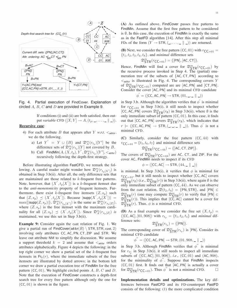
Fig. 4. Partial execution of FindCover. Explanation ofcircled A, B, C and D are provided in Example 9..

If conditions (i) and (ii) are both satisfied, then out-put variable CFD ([X, Y ] " A, (tp, , . . . , ! )).

Recursive case:4) For each attribute B that appears after Y w.r.t. <attr,we do the following.a) Let Y

!

= Y % {B} and DmA (rtp)[Y !] be the

difference sets of DmA (rtp)[Y ] not covered by B.

b) Call FindMin(A, (X, tp), Y!

, DmA (rtp)[Y !], <attr)

recursively following the depth-first strategy.

Before illustrating algorithm FastCFD, we remark the fol-lowing. A careful reader might wonder how Dm

A (rtp[X! ]) isobtained in Step 3.b(ii). After all, the only difference sets thatare maintained are those related to k-frequent free patterns.Note, however, that (X

!

, tp[X!

]) is a k-frequent itemset dueto the anti-monotonicity property of frequent itemsets. Fur-thermore, there exist k-frequent free itemsets (Z, sp) suchthat (Z, sp) , (X

!

, tp[X!

]). Because |supp(X!

, tp[X!

])| =max{|supp(Z, sp)|}, Dm

A (rtp[X! ]) is the same as DmA (rsp[Z]),

where (Z, sp) is the free itemset with the maximum cardi-nality for all (Z, sp) , (X

!

, tp[X!

]). Since DmA (rsp[Z]) is

maintained, we use this set in Step 3.b(ii).

Example 9: Consider again the cust relation of Fig. 1. Wegive a partial run of FindCover(attr(R) \ STR, STR, cust, 2)involving only attributes CC, AC, PN, CT, ZIP and STR. Weleave out attribute NM to simplify the discussion. We assumea support threshold k = 2 and assume that <attr ordersattributes alphabetically. Figure 4 depicts the following: in thetop right corner we show a partial set of the k-frequent freeitemsets in Frk(r), where the immediate subsets of the freeitemsets are illustrated by dotted arrows; in the bottom leftcorner we draw a partial execution tree of FindMin for the freepattern (CC, 01). We highlight circled points A, B, C and D.Note that the execution of FindCover constructs a depth-firstsearch tree for every free pattern although only the one for(CC, 01) is shown in the figure.

(A) As outlined above, FindCover passes free patterns toFindMin. Assume that the first free pattern to be consideredis 1. In this case, the execution of FindMin is exactly the sameas in the FastFD algorithm [14]. After this step all minimalFDs of the form (Y " STR, ( , . . . , ! )) are returned.

(B) Next, we consider the free pattern (CC, 01) with rCC=01 ={t1, t2, t3, t4, t8}, and minimal difference sets

DmSTR

(rCC=01) = {[PN], [AC, CT]}.

Hence, FindMin will find a cover for DmSTR

(rCC=01) bythe recursive process invoked in Step 4. The (partial) enu-meration tree of the subsets of {AC, CT, PN} according to<attr is illustrated in Fig. 4. The corresponding covers Yof Dm

STR(rCC=01) computed are are [AC, PN] and [CT, PN].

Consider the cover [AC, PN] and its minimal CFD candidate!

!

= ([CC, AC, PN] " STR, (01, , ! ))

in Step 3.b. Although the algorithm verifies that !! is minimalfor rCC=01 in Step 3.b(i), it still needs to inspect whether[CC, AC, PN] covers Dm

STR(r#) in Step 3.b(ii), where 1 is the

only immediate subset of pattern (CC, 01). In this case, it findsout that [CC, AC, PN] covers Dm

STR(r#), which indicates that

r |= ([CC, AC, PN] " STR, ( , , ! )). Thus !! is not a

minimal CFD.

(C) Similarly, consider the free pattern (CC, 44) withrCC=44 = {t5, t6, t7} and minimal difference sets

DmSTR

(rCC=44) = {[AC, CT, ZIP]}.

The covers of DmSTR

(rCC=44) are AC, CT, and ZIP. For thecover AC, FindMin needs to inspect if its CFD

! = ([CC, AC] " STR, (44, ! ))

is minimal. In Step 3.b(i), it verifies that ! is minimal forrCC=44, but it still needs to inspect whether [CC, AC] coversDm

STR(r#) (i.e., Dm

STR(r)) in Step 3.b(ii), where again 1 is the

only immediate subset of pattern (CC, 44). As we can observefrom the cust relation, D(t2, t4) = {PN, STR}, and [PN] $Dm

STR(r) (one may compute Dm

STR(r) to verify that [PN] $

DmSTR

(r)). This implies that [CC, AC] cannot be a cover forDm

STR(r). Thus, ! is a minimal CFD.

(D) As a final example we consider the free set (X, tp) =([CC, AC], [01, 908]) with rtp = {t1, t2, t4} and minimal dif-ference sets:

DmSTR

(rtp) = {[PN]}.

The corresponding cover of DmSTR

(rtp) is [PN]. Consider itsminimal CFD candidate

!!!

= ([CC, AC, PN] " STR, (01, 908, ! ))

in Step 3.b. Although FindMin verifies that !!! is minimalfor rtc

pin Step 3.b(i), it still needs to inspect all immediate

subsets of ([CC, AC], [01, 908]), i.e., (CC, 01) and (AC, 908),for the minimality of !

!! . Suppose that FindMin inspects(CC, 01) first. It finds out that [AC, PN] is actually a coverfor Dm

STR(rCC=01). Thus !

!! is not a minimal CFD. !

Implementation details and optimizations. The key dif-ferences between FastCFD and its FD-counterpart FastFDconsists of the following: (1) the more complicated condition

12

for testing the validity of a minimal CFD ! in terms of theminimality of the constant pattern and unnamed variables inLHS(!); and (2) the fact that we discover k-frequent CFDsinstead of 1-frequent FDs only. Whereas for FDs, the onlydifference sets needed are Dm

A (r) for A $ attr(R), Lemma 4states that for CFDs, difference setsDm

A (rtp) are needed for allrtp , where tp is a k-frequent free pattern in r. Worse still, when(X, tp) is reached, the depth-first approach enforces FindMin touse Dm

A (rtp[X!]) during the minimality check for all X ! + Xof size |X | 2 1. These suggest that we need a very efficientway to compute difference sets. To do so the following twoapproaches are implemented and evaluated.

NaiveFast. The first one is inspired by the stripped partitionidea used by FastFD [14]. Here for a given (X, tp), the strippedpartition of rtp w.r.t. an attribute A is the partition of rtp w.r.t.A from which all single-tuple equivalence classes are removed(see Section 4 for the definition of partition). The computationof the stripped partitions of rtp for each A $ attr(R) providessufficient information to infer for any two tuples on whichattributes they agree. By taking complements, one can theninfer the difference sets. It should be mentioned that thestripped partitions are often much smaller than the instances,making this approach efficient. We refer to the version thatrelies on the partition-based approach as NaiveFast.

FastCFD. The second approach relies on the availability ofClosed2(r), which consists of all 2-frequent closed itemsetsin r. Given (X, tp), we can again infer for any two tuplesin rtp on which attributes they agree. Indeed, these setsof attributes are given by the attributes in those itemsetsin Closed2(r) that match tcp (the constant part of tp). Bytaking the complement we can infer the desired differencesets efficiently. Our experimental study (Section 6) shows thatthis approach outperforms the partition-based approach and istherefore used to implement difference sets in FastCFD.Finally, since CFDMiner produces Closedk(r) as a side-

product, we use CFDMiner for constant CFD discovery andFastCFD for variable CFDs only. To do so, we eliminate Step3.a in FindCover. Taken together, these lead to significantimprovements in efficiency, as will be seen in the next section.

Dynamic attribute reordering. Similar to FastFD, FastCFDis equipped with a dynamic reordering of the attributes whenenumerating the subsets in the procedure FindMin. Morespecifically, instead of keeping <attr fixed throughout theexecution of FindMin, an additional step (between Step 4.aand Step 4.b) is included in which the remaining attributesare reordered based on a cost model.

FastCFD employs a cost model similar to FastFD, to dy-namically reorder attributes such that attributes that cover themost difference sets are treated first. We refer to [14] for moredetails concerning the cost model.

6 EXPERIMENTAL STUDYWe next present an experimental study of our algorithmsfor discovering minimal CFDs: CFDMiner, CTANE, NaiveFast,FastCFD given in Sections 3, 4 and 5, respectively. Weinvestigate the effects of the following factors on the scalability

and the number of minimal CFDs produced: (a) the supportthreshold k, (b) the size DBSIZE of a sample relation r,i.e., the number of tuples in r, (c) the arity ARITY of r, i.e., thenumber of columns in r, (d) a correlation factor (CF) [14],which indicates that the average range of distinct values in anattribute domain is CF 3 DBSIZE.

6.1 Experimental SettingsThe experiments were conducted on both real-life data and onsynthetic datasets generated using real data. Our experimentsused real datasets from the UCI machine learning repository(http://archive.ics.uci.edu/ml/), namely, the Wisconsin breastcancer (WBC) and Chess datasets. The following table de-scribes the parameters of those datasets:

Dataset Arity Size (# of tuples)Wisconsin breast cancer (WBC) 11 699

Chess 7 28,056Tax 14 20,000

To evaluate the scalability, we also used an extension of therelation in Fig. 1, which is a synthetic dataset for tax recordsgenerated by populating the database with data used in [1], viaa generator. The generator takes parameters ARITY, DBSIZEand CF, and produces datasets accordingly.The algorithms have been implemented in C++. The pro-

gram has been tested on AMD Opteron Processor (2.6GHZ)with 32GB of memory running the Linux operating system.Our algorithms run entirely in main memory. Each experimentwas repeated over 5 times and the average is reported here.

6.2 Experimental ResultsWe first present our experimental results on generated data,and then our results with real-life data.

Scalability Experiments. We study the performance of ouralgorithms by varying DBSIZE, ARITY, CF, and supportthreshold k in this set of experiments.

Scalability w.r.t. DBSIZE: Fixing ARITY = 7 and CF = 0.7we varied DBSIZE from 20K to 1 million tuples. We keptsupport ratio SUP%, which is defined as k

DBSIZE, at 0.1%.The response times of our algorithms are reported in Fig. 5.In particular, CFDMiner(2) indicates CFDMiner with k = 2,which is used in FastCFD for optimization.The results of Fig. 5 tell us the following. (a) CFDMiner,

which only mines constant CFDs, is multiple orders of mag-nitude faster than the other algorithms that discover bothconstant and variable CFDs. (b) The naive version of FastCFD,NaiveFast, outperforms CTANE when DBSIZE is small. How-ever, it does not scale well w.r.t. DBSIZE. For example, itoutperforms CTANE when DBSIZE is less than 100K . Butwhen DBSIZE is 300K , it is 2.5 times slower than CTANE.This behavior is primarily due to the cost incurred in theconstruction of the difference sets in NaiveFast. As observedfor FastFD [14], the difference set construction contributesmost to the cost of NaiveFast. When DBSIZE becomes larger,there are more itemsets with large support that need to beconsidered for constructing the difference sets. This results in a

13

0

100

200

300

400

500

0 200 400 600 800 1000

Resp

onse

tim

e (s

)

Number of tuples (x 1000)

FastCFDNaiveFast

CFDMiner(2)CTANE

CFDMiner

Fig. 5. Scalability w.r.t. DBSIZE

0

2

4

6

8

10

0 200 400 600 800 1000

Num

ber o

f CFD

s (x

100

0)

Number of tuples (x 1000)

Const + Var CFDsConst CFDs

Fig. 6. No. of CFDs found w.r.t. DBSIZE

0

100

200

300

400

500

600

7 9 11 13 15 17 19 21 23 25 27 29 31

Resp

onse

tim

e (m

inut

es)

Arity

CTANEFastCFD

NaiveFastCFDMiner

CFDMiner(2)

Fig. 7. Scalability w.r.t. ARITY

0

50

100

150

200

250

300

350

50 75 100 125 150

Resp

onse

Tim

e (s

)

Support (DB size=100k, arity=7)

CTANENaiveFastCFDMinerFastCFD

CFDMiner(2)

Fig. 8. Scalability w.r.t. k

0

2

4

6

8

10

12

14

50 75 100 125 150

Num

ber o

f CFD

s (x

100

0)

Support (DB size=100k, arity=7)

Const+Var CFDsConst CFDs

Fig. 9. No. of CFDs found w.r.t. k

0

10

20

30

40

50

60

70

0.3 0.5 0.7

Resp

onse

tim

e (m

inut

es)

CF

CTANENaiveFastFastCFD

Fig. 10. Scalability w.r.t. CF

0

20

40

60

80

100

0 10 20 30 40

Resp

onse

tim

e (s

)

Support

FastCFDCTANE

Fig. 11. Wisc. breast cancer

0

100

200

300

400

500

600

700

30 60 90 120

Resp

onse

tim

e (s

)

Support

FastCFDCTANE

Fig. 12. Chess

0

50

100

150

200

250

300

0 50 100 150 200 250 300

Resp

onse

tim

e (s

)

Support

FastCFDCTANE

Fig. 13. Tax

significant performance degradation of NaiveFast. (c) FastCFDoutperforms CTANE and NaiveFast when DBSIZE is less thanone million tuples, which is reasonably large. This verifiesthe effectiveness of our optimization by leveraging the closed-itemsets from CFDMiner for constructing difference sets.

Figure 6 shows the total number of minimal CFDs discov-ered by our algorithms. For clarity, only constant and variableCFDs of FastCFD are shown because CTANE, NaiveFast andFastCFD find about the same number of CFDs.

Scalability w.r.t. ARITY: Fixing CF = 0.7, DBSIZE = 20K ,and SUP% = 0.1%, we varied ARITY from 7 to 31. As shownin Fig. 7, CTANE does not scale well with the arity, as ex-pected. In contrast, NaiveFast and FastCFD scale well: both are

orders of magnitude better than CTANE when ARITY * 15.In addition, FastCFD is 4 times better than NaiveFast whenARITY = 31, which further demonstrates the effectiveness ofthe optimization techniques of FastCFD via CFDMiner.

Scalability w.r.t. k: We fixed CF = 0.7, DBSIZE = 100K ,SUP% = 0.1%, and varied the support threshold k from 50to 150. As shown in Fig. 8, NaiveFast and FastCFD onlyimprove slightly when k increases. In contrast, CTANE ishighly sensitive to k. For example, NaiveFast outperformsCTANE when k is small (e.g., 50), whereas CTANE outper-forms NaiveFast when k is large (e.g., 150). The performanceof CTANE improves as k increases. This is because feweritemsets with large support satisfy k when k becomes larger,

14

0

500

1000

1500

2000

2500

3000

10 20 30 40

Num

ber o

f CFD

s

Support

Fig. 14. Wisc. breast cancer

0

300

600

900

1200

1500

1800

30 60 90 120

Num

ber o

f CFD

s

Support

Fig. 15. Chess

0

1000

2000

3000

4000

5000

6000

50 100 150 200 250 300

Num

ber o

f CFD

s

Support

Fig. 16. Tax

which certainly reduces the number of candidates to examineat each level by CTANE. On the other hand, the main cost forNaiveFast and FastCFD is in the construction of differencesets for itemsets with large support, which does not changesignificantly when k gets larger.Figure 9 shows that the number of minimal CFDs discovered

decreases as k increases, as expected. Again, only constantand variable CFDs of FastCFD are shown because CTANE,NaiveFast and FastCFD find about the same number of CFDs.

Scalability w.r.t. CF: We varied CF from 0.3 to 0.7, whilefixing DBSIZE = 50K , k = 50 and ARITY = 9. Asshown in Fig. 10, CTANE is very sensitive to the number ofdistinct values in an attribute domain. As we fixed the totalnumber of tuples at 50K , when CF decreases, the number ofitemsets with large support increases. For a fixed k, this meansmore itemsets satisfying the support threshold in CTANE.Thus the algorithm has to examine more candidates at eachlevel, which leads to performance degradation. In contrast, theperformance of NaiveFast and FastCFD only degrades slightlyas CF decreases.

Real Data Experiments We have conducted experiments onreal-life data, including the Chess, WBC, and synthetic Taxdatasets. For each dataset, k was varied. Figures 11, 12, 13show the response times of CTANE and FastCFD when k isvaried, while figures 14, 15 and 16 show the correspondingnumbers of CFDs discovered by the algorithms. Consistentwith our previous experiments, CTANE is sensitive to thesupport threshold k, and its performance improves when kincreases. FastCFD is less sensitive to k, and its performanceonly improves slightly as k increases. Both algorithms discoverfewer number of CFDs as k increases.

Summary. From the experimental results we find the follow-ing. (a) Constant CFD discovery (CFDMiner) can be multi-ple orders of magnitude faster than general CFD discovery(CTANE or FastCFD). (b) CTANE usually works well when thearity of a relation is small and the support threshold is large,but it scales poorly when the arity increases. (c) NaiveFast andFastCFD are far more efficient than CTANE when the arityof the relation is large. (d) Our optimization technique basedon closed-itemset mining is effective: FastCFD significantlyoutperforms NaiveFast, especially when the arity is large.

7 RELATED WORK

Prior work on conditional dependencies has mostly focusedon the consistency and implication analyses of CFDs [1],repairing methods to localize and fix errors detected by CFDs[26], propagation of CFDs from source data to views in dataintegration [27], extensions of CFDs by adding disjunction andnegation [28] or adding ranges [10], confidence of CFDs [29],as well as extensions of inclusion dependencies with condi-tions (referred to as CINDs) [30]. To our knowledge, CFDdiscovery was only studied in [21], [10], [31]. Except these,the previous work assumes that CFDs are already designedand provided.As remarked in Section 1, there has been a host of work

on minimal FD discovery [12], [13], [14], [15], [16], [17],[18]. Minimal CFDs, however, are more involved than their FDcounterparts: they require both the minimality of attributes andthe minimality of patterns (Section 2). Our algorithms CTANEand FastCFD extend TANE [13] and FastFD [14], respectively,for discovering minimal CFDs.Closer to our work are [10], [21], [31]. For a fixed traditional

FD, [10] proposed criteria for sensible patterns that, togetherwith the FD, make useful CFDs. It showed that the problem offinding such patterns is NP-complete, and developed efficientheuristic algorithms for discovering patterns from samples.In contrast to [10], this work studies CFD discovery whenthe embedded traditional FDs are not given. An algorithmfor discovering CFDs is developed in [21], which aims tofind both traditional FDs and patterns in CFDs, the same aswhat this work does. Several interest measures for discoveredCFDs are also proposed there, including support (which wealso consider), conviction and (2-test. The algorithm of [21]differs from our algorithms in the following aspects. (a) Thealgorithm of [21] is an extension of TANE [13]; as shown inSection 6, levelwise CFD-discovery algorithms may not scalewell with the arity of sample datasets. It is to deal with suchdata that FastCFD is provided. In contrast, this issue is notaddressed in [21]. (b) In addition, constant CFD discovery isnot considered in [21], despite its wide applications in datacleaning and data integration. (c) Moreover, [21] does notconsider optimizations based on closed itemsets mining, whichis employed by FastCFD.As observed in Sections 1 and 3, CFD discovery is also

15

closely related to (non-redundant) association rule mining [22],[23], [24]. In particular, CFDMiner is based on the mining al-gorithm proposed in [24]. Recently an algorithm was proposedin [31] for mining association rules of the form Q1 # Q2,where Q1, Q2 are simple conjunctive queries and Q2 iscontained inQ1. Since CFDs and CINDs can be viewed as suchassociation rules, the algorithm of [31] may be used to minegeneral CFDs and CINDs. The method of [31], however, canonly discover CFDs with 100% confidence, and in addition,the minimality of CFDs is not investigated in [31]. In contrast,the algorithms of this work are developed to discover minimalk-frequent CFDs. The connection between association rulemining and constant CFD discovery is also observed in [32].Neither [31] nor [32] provides any experimental results.

8 CONCLUSIONSWe have developed and implemented three algorithms fordiscovering minimal CFDs: (1) CFDMiner for mining minimalconstant CFDs, a class of CFDs important for both datacleaning and data integration; (2) CTANE for discoveringgeneral minimal CFDs based on the levelwise approach; and(3) FastCFD for discovering general minimal CFDs based on adepth-first search strategy, and a novel optimization techniquevia closed-itemset mining. As suggested by our experimentalresults, these provide a set of tools for users to choose fordifferent applications. When only constant CFDs are needed,one can simply use CFDMiner without paying the price ofmining general CFDs. When the arity of a sample dataset islarge, one should opt for FastCFD. When k-frequent CFDs areneeded for a large k, one could use CTANE.There is naturally much to be done. First, we are currently

experimenting with various datasets collected from real life.Second, we are investigating how to discover minimal CFDsfrom a dataset r when both its arity and its size are large.To our knowledge, no dependency discovery algorithms scalevery well in this setting, even those for traditional FDs. Oneway around this is by sampling r, i.e., to find a subset rs ofr by selectively drawing tuples from r such that rs accuratelyrepresents r and is small enough to be efficiently processedby FastCFD or CTANE. It is, however, nontrivial to find asampling method with performance guarantee, i.e., to ensurethat the estimated inaccuracy rate is below a predefined boundwith high confidence. We are experimenting with the stratifiedsampling method [33] for this purpose. Third, while we haveemployed in FastCFD techniques for mining closed itemsets,we expect that other mining techniques may also shed light inimproving the performance of discovery algorithms. Fourth,we plan to explore the use of CFD inference in discovery, toeliminate CFDs that are entailed by those CFDs already found.Finally, while the focus of this work is on algorithmic issuesfor mining CFDs, a topic for future work is to assess qualitymeasures for CFDs, including those studied in [10], [21].

REFERENCES[1] W. Fan, F. Geerts, X. Jia, and A. Kementsietsidis, “Conditional func-

tional dependencies for capturing data inconsistencies,” TODS, vol. 33,no. 2, june 2008.

[2] G. Cong, W. Fan, F. Geerts, X. Jia, and S. Ma, “Improving data quality:Consistency and accuracy,” in VLDB, 2007.

[3] M. Arenas, L. E. Bertossi, and J. Chomicki, “Consistent query answersin inconsistent databases,” TPLP, vol. 3, no. 4-5, pp. 393–424, 2003.

[4] J. Chomicki and J. Marcinkowski, “Minimal-change integrity mainte-nance using tuple deletions,” Information and Computation, vol. 197,no. 1-2, pp. 90–121, 2005.

[5] J. Wijsen, “Database repairing using updates,” TODS, vol. 30, no. 3, pp.722–768, 2005.

[6] C. Batini and M. Scannapieco, Data Quality: Concepts, Methodologiesand Techniques. Springer, 2006.

[7] E. Rahm and H. H. Do, “Data cleaning: Problems and current ap-proaches.” IEEE Data Eng. Bull., vol. 23, no. 4, pp. 3–13, 2000.

[8] Gartner, “Forecast: Data quality tools, worldwide, 2006-2011,” 2007.[9] S. Abiteboul, R. Hull, and V. Vianu, Foundations of Databases.

Addison-Wesley, 1995.[10] L. Golab, H. Karloff, F. Korn, D. Srivastava, and B. Yu, “On generat-

ing near-optimal tableaux for conditional functional dependencies,” inVLDB, 2008.

[11] E.-P. Lim, J. Srivastava, S. Prabhakar, and J. Richardson, “Entityidentification in database integration,” Inf. Sci., vol. 89, no. 1-2, pp.1–38, 1996.

[12] H. Mannila and K.-J. Raiha, “Dependency inference,” in VLDB, 1987.[13] Y. Huhtala, J. Karkk ainen, P. Porkka, and H. Toivonen, “TANE: An

efficient algorithm for discovering functional and approximate depen-dencies,” Comput. J., vol. 42, no. 2, pp. 100–111, 1999.

[14] C. M. Wyss, C. Giannella, and E. L. Robertson, “FastFDs: A heuristic-driven, depth-first algorithm for mining functional dependencies fromrelation instances - extended abstract,” in DaWak, 2001.

[15] P. A. Flach and I. Savnik, “Database dependency discovery: A machinelearning approach,” AI Commun., vol. 12, no. 3, pp. 139–160, 1999.

[16] S. Lopes, J.-M. Petit, and L. Lakhal, “Efficient discovery of functionaldependencies and armstrong relations,” in EDBT, 2000.

[17] T. Calders, R. T. Ng, and J. Wijsen, “Searching for dependencies atmultiple abstraction levels,” TODS, vol. 27, no. 3, pp. 229–260, 2003.

[18] R. S. King and J. J. Legendre, “Discovery of functional and approximatefunctional dependencies in relational databases,” JAMDS, vol. 7, no. 1,pp. 49–59, 2003.

[19] I. F. Ilyas, V. Markl, P. J. Haas, P. Brown, and A. Aboulnaga, “Cords:Automatic discovery of correlations and soft functional dependencies,”in SIGMOD, 2004.

[20] H. Mannila and H. Toivonen, “Levelwise search and borders of theoriesin knowledge discovery,” Data Min. Knowl. Discov., vol. 1, no. 3, pp.259–289, 1997.

[21] F. Chiang and R. Miller, “Discovering data quality rules,” in VLDB,2008.

[22] R. Agrawal, H. Mannila, R. Srikant, H. Toivonen, and A. I. Verkamo,“Fast discovery of association rules,” in Advances in Knowledge Dis-covery and Data Mining, 1996.

[23] M. J. Zaki, “Mining non-redundant association rules,” Data Min. Knowl.Discov., vol. 9, no. 3, pp. 223–248, 2004.

[24] J. Li, G. Liu, and L. Wong, “Mining statistically important equivalenceclasses and delta-discriminative emerging patterns,” in KDD, 2007.

[25] H. Li, J. Li, L. Wong, M. Feng, and Y.-P. Tan, “Relative risk and oddsratio: a data mining perspective,” in PODS, 2005.

[26] G. Cong, W. Fan, F. Geerts, X. Jia, and S. Ma, “Improving data quality:Consistency and accuracy,” in VLDB, 2007.

[27] W. Fan, S. Ma, Y. Hu, J. Liu, and Y. Wu, “Propagating functionaldependencies with conditions,” in VLDB, 2008.

[28] L. Bravo, W. Fan, F. Geerts, and S. Ma, “Increasing the expressivity ofconditional functional dependencies without extra complexity,” in ICDE,2008.

[29] G. Cormode, L. Golab, F. Korn, A. McGregor, D. Srivastava, andX. Zhang, “Estimating the confidence of conditional functional depen-dencies,” in SIGMOD, 2009.

[30] L. Bravo, W. Fan, and S. Ma, “Extending dependencies with conditions,”in VLDB, 2007.

[31] B. Goethals, W. L. Page, and H. Mannila, “Mining association rules ofsimple conjunctive queries,” in SDM, 2008.

[32] R. Medina and N. Lhouari, “A unified hierarchy for functional depen-dencies, conditional functional dependencies and association rules,” inICFCA, 2009.

[33] N. Alon and J. H. Spencer, “The Probabilistic Method”. John WileyInc., 1992.