discontinuous galerkin methods for elliptic partial differential equations with random coefficients
TRANSCRIPT

This article was downloaded by: [Aston University]On: 04 October 2014, At: 23:08Publisher: Taylor & FrancisInforma Ltd Registered in England and Wales Registered Number: 1072954 Registeredoffice: Mortimer House, 37-41 Mortimer Street, London W1T 3JH, UK
International Journal of ComputerMathematicsPublication details, including instructions for authors andsubscription information:http://www.tandfonline.com/loi/gcom20
Discontinuous Galerkin methods forelliptic partial differential equationswith random coefficientsKun Liua & Béatrice M. Rivièrea
a Computational and Applied Mathematics Department, RiceUniversity, 6100 Main Street, Houston, TX 77005, USAAccepted author version posted online: 19 Mar 2013.Publishedonline: 16 Apr 2013.
To cite this article: Kun Liu & Béatrice M. Rivière (2013) Discontinuous Galerkin methods forelliptic partial differential equations with random coefficients, International Journal of ComputerMathematics, 90:11, 2477-2490, DOI: 10.1080/00207160.2013.784280
To link to this article: http://dx.doi.org/10.1080/00207160.2013.784280
PLEASE SCROLL DOWN FOR ARTICLE
Taylor & Francis makes every effort to ensure the accuracy of all the information (the“Content”) contained in the publications on our platform. However, Taylor & Francis,our agents, and our licensors make no representations or warranties whatsoever as tothe accuracy, completeness, or suitability for any purpose of the Content. Any opinionsand views expressed in this publication are the opinions and views of the authors,and are not the views of or endorsed by Taylor & Francis. The accuracy of the Contentshould not be relied upon and should be independently verified with primary sourcesof information. Taylor and Francis shall not be liable for any losses, actions, claims,proceedings, demands, costs, expenses, damages, and other liabilities whatsoever orhowsoever caused arising directly or indirectly in connection with, in relation to or arisingout of the use of the Content.
This article may be used for research, teaching, and private study purposes. Anysubstantial or systematic reproduction, redistribution, reselling, loan, sub-licensing,systematic supply, or distribution in any form to anyone is expressly forbidden. Terms &Conditions of access and use can be found at http://www.tandfonline.com/page/terms-and-conditions
International Journal of Computer Mathematics, 2013Vol. 90, No. 11, 2477–2490, http://dx.doi.org/10.1080/00207160.2013.784280
Discontinuous Galerkin methods for elliptic partial differentialequations with random coefficients
Kun Liu and Béatrice M. Rivière*
Computational and Applied Mathematics Department, Rice University, 6100 Main Street, Houston,TX 77005, USA
(Received 25 October 2012; revised version received 4 March 2013; accepted 6 March 2013 )
This paper proposes and analyses two numerical methods for solving elliptic partial differential equationswith random coefficients, under the finite noise assumption. First, the stochastic discontinuous Galerkinmethod represents the stochastic solution in a Galerkin framework. Second, the Monte Carlo discontin-uous Galerkin method samples the coefficients by a Monte Carlo approach. Both methods discretize thedifferential operators by the class of interior penalty discontinuous Galerkin methods. Error analysis isobtained. Numerical results show the sensitivity of the expected value and variance with respect to thepenalty parameter of the spatial discretization.
Keywords: stochastic discontinuous Galerkin; finite noise; stochastic elliptic equation; Monte Carlosimulation; a priori error estimate
2010 AMS Subject Classifications: 65N30; 65N15; 65C05; 65C20; 65N12
1. Introduction
The numerical solution of stochastic partial differential equations is an active area of research,and has many applications in engineering. For instance, in porous media flow, uncertainty in thepermeability of the medium yields a stochastic elliptic problem for the Darcy model. For givenstochastic functions a, f : � × D → R, the solution to the stochastic elliptic problem satisfiesalmost surely
−∇ · (a(ω, ·)∇u(ω, ·)) = f (ω, ·), in D, (1)
u(ω, ·) = 0, on ∂D. (2)
Here, D is a polygonal domain in Rd , d = 2, 3 and (�, F , P) is a probability space. The stochasticcoefficient a is assumed to be uniformly bounded
0 < a0 ≤ a(w, x) ≤ a1, a.e. � × D. (3)
Under the assumption of finite-dimensional noise (justified for instance by the use of truncatedKarhunen–Loève [15]), the stochastic elliptic problem is reduced to a parametrized one. Wewrite a(ω, x) = a(Y(ω), x) and f (ω, x) = f (Y(ω), x), with Y(ω) = (Y1(ω), . . . , YN (ω)) being a
*Corresponding author. Email: [email protected]
© 2013 Taylor & Francis
Dow
nloa
ded
by [
Ast
on U
nive
rsity
] at
23:
08 0
4 O
ctob
er 2
014
2478 K. Liu and B.M. Rivière
vector of random variables. We assume that the range of Yi is a bounded interval �i and we denote� = �N
i=1�i. The function ρ denotes the joint probability density of Y . The resulting parametrizedelliptic problem is
−∇ · (a(y, x)∇u(y, x)) = f (y, x), ∀(y, x) ∈ � × D, (4)
u(y, x) = 0, ∀(y, x) ∈ � × ∂D. (5)
We propose two numerical methods for solving Equations (4) and (5): the stochastic discontin-uous Galerkin (SDG) method and the Monte Carlo discontinuous Galerkin (MCDG) method.The two methods differ in the treatment of the uncertainty. This paper points out the advan-tages and disadvantages of each method. The common denominator is the spatial discretization.The class of interior penalty discontinuous Galerkin methods [18] is employed. These methodshave been shown to be well-suited for porous media flows, with deterministic discontinuouspermeability [19]. There are three variations of the interior penalty methods: symmetric [2,22],non-symmetric [20] and incomplete [8]. In this work, we show the effects of uncertainty on thechoice of discretization. In particular, we discuss the numerical advantages and disadvantages ofusing the non-symmetric MCDG versus the symmetric MCDG.
Our paper can be related to the work of [4] where the classical finite element methods are usedto solve stochastic elliptic problems. Our paper differs in the fact that discontinuous Galerkin(DG) methods are employed for the spatial discretization techniques. As a result, the analysis ofthe proposed method uses different techniques. Several stochastic finite element methods havebeen proposed and analysed in the literature: see for instance [5,9,11,13,14,16] and the referencestherein. Collocation methods have also been studied in the context of stochastic partial differentialequations [3,17,23]. Collocation methods are known to converge faster than Monte Carlo methods,but they require special quadrature rules for optimal rates.
There is very little published literature on the formulation and analysis of SDG methods. In [24],the local discontinuous Galerkin (LDG) method is applied to the Poisson problem with white noisein the source function and in [7], the same approach is applied to Helmholtz problems. The LDGmethod is another class of DG methods, that uses a mixed formulation of the problem, and iswell-suited to hyperbolic problems.
An outline of the paper is as follows. Section 2 introduces the SDG method. Theoreticalconvergence results are proved. Section 3 defines the MCDG method and provides an erroranalysis. Some numerical examples for the MCDG are given in Section 4. Conclusions follow.
2. SDG methods
2.1 Scheme
The outcome set � is partitioned into a finite number of disjoint boxes of maximum size k. Theresulting mesh is denoted by Fk . The spatial domain D is partitioned into elements (triangles andparallelograms in 2D, tetrahedra or hexahedra in 3D) with maximum diameter h. The family ofmeshes, denoted by Th, is assumed to be shape regular. Denote by �h the set of interior edges (orfaces) of the subdivision Th. With each edge (or face) e, we associate a unit normal vector ne. Ife is on the boundary ∂D, then ne is the outward vector normal to ∂D. If two elements T e
1 and T e2
are neighbours with one common side e, there are two traces of u along e. We also assume thatthe normal vector ne is oriented from T e
1 to T e2 , and defines the average and jump as
{u} = 12 (u|Te
1) + 1
2 (u|Te2), [u] = (u|Te
1) − (u|Te
2), ∀e = ∂T e
1 ∩ ∂T e2 .
Dow
nloa
ded
by [
Ast
on U
nive
rsity
] at
23:
08 0
4 O
ctob
er 2
014

International Journal of Computer Mathematics 2479
We extend the definition to sides or faces that belong to the boundary ∂D
{u} = [u] = u|Te1, ∀e = ∂T e
1 ∩ ∂D.
We now define the bilinear form A corresponding the interior penalty method
A(y; u, v) =∑T∈Th
∫T
a(y, ·)∇u · ∇v −∑
e∈�h∪∂D
∫e{a(y, ·)∇u · ne}[v]
+ ε∑
e∈�h∪∂D
∫e{a(y, ·)∇v · ne}[u] +
∑e∈�h∪∂D
σe
h
∫e[u][v]. (6)
The discrete space for the SDG method is the tensor product space V qk ⊗ Dr
h
V qk ⊗ Dr
h = {ψ ∈ L2(� × D) : ψ ∈ span(ϕ(y)χ(x) : ϕ ∈ V qk , χ ∈ Dr
h)}, (7)
where Drh is the space of piecewise discontinuous polynomials of degree r over the partition Th
Drh = {v ∈ L2(D) : ∀T ∈ Th, v|T ∈ Pr(T)}, (8)
and V qk is the space of discontinuous polynomials of degree q in each direction over the
partition Fk
V qk = {v ∈ L2(�) : ∀γ ∈ Fk , v|γ ∈ Qq(γ )}. (9)
The SDG method is defined as follows: find uhk ∈ V qk ⊗ Dr
h satisfying
∫�
ρ(y)A(y; ukh, v) dy =∫
�
ρ(y)(f , v)D dy, ∀v ∈ V qk ⊗ Dr
h. (10)
Assume that the parameters r, ε and σe are chosen so that they satisfy one of the following fourassumptions:
Case 1: In the non-symmetric case (ε = 1), r ≥ 1 and σe = 1 for all faces e; this method isreferred to as the non-symmetric interior penalty Galerkin method.
Case 2: In the symmetric case (ε = −1), r ≥ 1 and σe is large enough; this method is referredto as the symmetric interior penalty Galerkin method.
Case 3: In the incomplete case (ε = 0), r ≥ 1 and σe is large enough; this method is referredto as the incomplete interior penalty Galerkin method.
Case 4: In the non-symmetric case (ε = 1), r ≥ 2 and σe = 0 for all faces e.
For cases 2 and 3, the penalty value σe varies over each face and one can easily see that theminimum values for deterministic problems are valid for the parametrized elliptic problem. Thereader can refer to [1,10,21] and the references herein for various computable lower bounds ofthe penalty parameter. We now recall the minimum penalty values for stable DG solutions of 2Dproblems, given in [10]. Let e be an interior edge shared by two triangles E1
e and E2e . Let θi denote
the smallest angle of triangle Eie and let ai
0 (respectively, ai1) denote the minimum (respectively,
Dow
nloa
ded
by [
Ast
on U
nive
rsity
] at
23:
08 0
4 O
ctob
er 2
014

2480 K. Liu and B.M. Rivière
maximum) value of the stochastic coefficient a in the element Eie. The threshold value for the
penalty parameter is
σe = r(r + 1)
(3(a1
1)2
2a10
cot θ1 + 3(a21)
2
2a20
cot θ2
). (11)
A similar expression is obtained for a boundary edge e ∈ ∂E1e
σe = 6(a11)
2
a10
r(r + 1) cot θ1. (12)
We now define the energy norm ‖ · ‖E
‖u‖2DG =
∑T∈Th
∫T(∇u)2 +
∑e∈�h∪∂D
1
h
∫e[u]2,
‖u‖E =(∫
�
ρ(y)‖u(y, ·)‖2DG dy
)1/2
.
The property (3) and the assumptions above on r, ε, and σe imply coercivity of the form A [18],which then yields coercivity of the form
∫�
ρA(y; ·, ·)dy. There is a positive constant α > 0 suchthat
α‖v‖2E ≤
∫�
ρA(y; v, v) dy, ∀v ∈ V qk ⊗ Dr
h. (13)
Existence and uniqueness of the linear finite-dimensional problem (10) follow from this coercivityresult. We finally remark that the scheme is consistent, i.e. the exact solution u ∈ L2(�; Hs(D)) ∩Hq+1(�; H1
0 (D)) (for s ≥ 2) satisfies Equation (10).
2.2 Error analysis
In this section, a priori error estimates are obtained with respect to the discretization parametersk and h. The following approximation result can be easily obtained from [4].
Lemma 2.1 Let u ∈ L2(�; Hs(D)) ∩ Hq+1(�; H10 (D)) for s ≥ 2, q ≥ 0 and let r ≥ 0 be an inte-
ger. There exists a constant C independent of u, h and k and a function u ∈ V qk ⊗ Dr
h such that
‖∇(u − u)‖L2(�;L2(Th)) ≤ Chmin(r+1,s)−1‖u‖L2(�;Hs(D)) + Ckq+1N∑
i=1
‖∂q+1yi
u‖L2(�;H10 (D)) (14)
and
‖∇2(u − u)‖L2(�;L2(Th)) ≤ Chmin(r+1,s)−2‖u‖L2(�;Hs(D)) + Ch−1kq+1N∑
i=1
‖∂q+1yi
u‖L2(�;H10 (D)). (15)
In addition, u can be chosen so that it is continuous over D and vanishes on the boundary ∂D.
The next theorem states that the SDG solution converges optimally to the exact solution in theenergy norm.
Dow
nloa
ded
by [
Ast
on U
nive
rsity
] at
23:
08 0
4 O
ctob
er 2
014
International Journal of Computer Mathematics 2481
Theorem 2.2 Let u ∈ L2(�; Hs(D)) ∩ Hq+1(�; H10 (D)) for s ≥ 2, q ≥ 0, be a solution to Equa-
tions (4) and (5) and let ukh ∈ V qk ⊗ Dr
h be a solution to Equation (10). There is a constant Cindependent of h, k and u, such that
‖u − ukh‖E ≤ C
(hmin(r+1,s)−1‖u‖L2(�;Hs(D)) + kq+1
N∑i=1
‖∂q+1yi
u‖L2(�;H10 (D))
). (16)
Proof We first estimate the error ‖χ‖E with χ = ukh − u. Using the coercivity property (13) andthe consistency of the scheme, we have
α‖ukh − u‖2E ≤
∫�
ρA(y; ukh − u, ukh − u) dy +∫
�
ρA(y; u − ukh, ukh − u) dy
=∫
�
ρ
⎛⎝∑
T∈Th
∫E
a∇(u − u)∇χ −∑
e∈�h∪∂D
∫e{a∇(u − u) · ne}[χ ]
+ ε∑
e∈�h∪∂D
∫e{a∇χ · ne}[u − u] +
∑e∈�h∪∂D
σe
h
∫e[u − u][χ ]
)dy
≤ |T1 + T2 + T3 + T4|.To bound the terms Ti, for i = 1, . . . , 4, we use techniques standard to the analysis of interiorpenalty discontinuous Galerkin methods. Details can be found in [18]. We briefly state the results.The terms T3 and T4 vanish because u is continuous and vanishes on the boundary of D. The termsT1 and T2 are bounded by
T1 ≤ C‖u − u‖2L2(�;H1
0 (D))+ α
4‖χ‖2
E ,
T2 ≤ C
⎛⎝‖u − u‖2
L2(�;H10 (D))
+∑T∈Th
h‖∇2(u − u)‖2L2(T)
⎞⎠ + α
4‖χ‖2
E .
The constant C is independent of u, u and h, k but depends on the coercivity constant α, thepenalty parameter σe and the upper bound a1 of the coefficient a. Using the approximation resultsof Lemma 2.1, we obtain
‖ukh − u‖E ≤ Chmin(r+1,s)−1‖u‖L2(�;Hs(D)) + Ckq+1N∑
i=1
‖∂q+1yi
u‖L2(�;H10 (D)).
The final result is obtained by the triangle inequality
‖u − ukh‖E ≤ ‖u − u‖E + ‖ukh − u‖E
and the approximation bounds of Lemma 2.1. �
The next result estimates the expected value of the solution. We recall the definition of theexpected value.
E[v](·) =∫
�
ρ(y)v(y, ·) dy.
Dow
nloa
ded
by [
Ast
on U
nive
rsity
] at
23:
08 0
4 O
ctob
er 2
014
2482 K. Liu and B.M. Rivière
Theorem 2.3 Assume that D is a convex domain, that ε = −1 and that the assumptions ofTheorem 2.2 hold. Then, there is a constant C independent of h, k and u, such that
‖E[u − ukh]‖L2(D) ≤ C(h + kq+1)
(hmin(r+1,s)−1‖u‖L2(�;Hs(D))
+kq+1N∑
i=1
‖∂q+1yi
u‖L2(�;H10 (D))
). (17)
Proof The argument for the proof involves the solution to a dual problem.
−∇ · (a(y, x)∇�(y, x)) = E[u − ukh](x), ∀(y, x) ∈ � × D,
�(y, x) = 0, ∀(y, x) ∈ � × ∂D.
Elliptic regularity [4] implies existence of a constant C that depends on the domain D and thecoefficient a, such that
‖�(y, ·)‖H2(D) + ‖∂q+1yi
�(y, ·)‖H10 (D) ≤ C‖E[u − ukh]‖L2(D), ∀y ∈ �, ∀i = 1, . . . , N . (18)
Therefore, we have by denoting η = u − ukh
‖E[u − ukh]‖2L2(D) =
∫�
ρ(y)(E[η], η(y, ·))D dy
=∫
�
ρ(y) − ∇ · (a(y, ·)∇�(y, ·)), η(y, ·)D dy.
Integrating by parts on each element yields
‖E[η]‖2L2(D) =
∫�
ρ(y)∑T∈Th
∫T
a(y)∇�(y) · ∇η(y) dy
−∫
�
ρ(y)∑
e∈�h∪∂D
∫e{a(y)∇�(y) · ne}[η(y)] dy. (19)
Consistency of the scheme implies that∫�
ρ(y)A(y; η, v) dy = 0, ∀v ∈ V qk ⊗ Dr
h. (20)
Subtracting Equation (20) from Equation (19) and using the fact that ε = −1, we have
‖E[η]‖2L2(D) =
∫�
ρ∑T∈Th
∫T
a∇(� − v) · ∇η dy −∫
�
ρ∑
e∈�h∪∂D
∫e{a∇(� − v) · ne}[η] dy
+∫
�
ρ∑
e∈�h∪∂D
∫e{a∇η · ne}[v] dy −
∫�
ρ∑
e∈�h∪∂D
σe
h
∫e[η][v] dy. (21)
Choose v = �, an approximation of �, satisfying Lemma 2.1. The last two terms in the right-hand side of Equation (21) vanish. The first two terms are bounded by using trace inequalities
Dow
nloa
ded
by [
Ast
on U
nive
rsity
] at
23:
08 0
4 O
ctob
er 2
014

International Journal of Computer Mathematics 2483
and Caucy–Schwarz’s inequality. We have
‖E[η]‖2L2(D) ≤ C(‖∇(� − �)‖L2(�;L2(Th)) + h‖∇2(� − �)‖L2(�;L2(Th)))‖η‖E .
We then obtain by using the approximation bounds (14), (15) and (18)
‖E[η]‖2L2(D) ≤ C(h + kq+1)‖E[η]‖‖η‖E ,
and the final result is obtained with Theorem 2.2. �
Remark 1 Because of the Galerkin framework, theoretical convergence of the SDG methodis relatively easy to obtain. However, these methods become computationally expensive as thedimension of the outcome space increases. In addition, they are not as easily parallelizable as theMonte Carlo methods. Therefore, in the next section, we formulate a MCDG method.
3. MCDG methods
3.1 Scheme
In this section, the Monte Carlo sampling technique is combined with the discontinuous Galerkindiscretization. The notation is defined in Section 2.1. The MCDG method consists of the followingsteps:
• Choose a number of realizations M ∈ N+ and a finite dimensional space Drh.
• For each j = 1, . . . , M, sample independent, identically distributed (iid) realizations of thecoefficient a(yj, ·), the source function f (yj, ·) and find an approximation uh(yj, ·) ∈ Dr
h suchthat
A(yj; uh(yj, ·), v) = (f (yj, ·), v)L2(D), ∀v ∈ Drh. (22)
• Approximate the expected value E[u(·, ·)] by the sample average
SMuh(x) = 1
M
M∑j=1
uh(yj, x), x ∈ D. (23)
3.2 Error analysis
The computational error is naturally split into a space discretization error ηh and a statisticalerror ηM
E[u] − SMuh = (E[u] − E[uh]) + (E[uh] − SMuh) ≡ ηh + ηM .
The space discretization error ηh is controlled by the size of the spatial triangulation, while thestatistical error ηM is controlled by the number of realizations.
Lemma 3.1 There is a constant C > 0 independent of M and h such that
E[‖ηM‖2DG] <
C
M. (24)
Dow
nloa
ded
by [
Ast
on U
nive
rsity
] at
23:
08 0
4 O
ctob
er 2
014
2484 K. Liu and B.M. Rivière
Proof We note that the norm ‖ · ‖DG results from the following inner-product:
〈v, w〉 =∑T∈Th
(∇v, ∇w)T +∑
e∈�h∪∂D
1
h([v], [w])e.
Then, we write
E[‖ηM‖2DG] = E
⎡⎣
⟨1
M
M∑i=1
(E[uh] − uh(yi)),1
M
M∑j=1
(E[uh] − u(yj))
⟩⎤⎦
= 1
M2
M∑i,j=1
E[〈E[uh] − uh(yi), E[uh] − uh(yj)〉]
= 1
M2
M∑i=1
E[〈E[uh] − uh(yi), E[uh] − uh(yi)〉].
The last equality is due to the fact that since the realizations are iid, the expected value of 〈E[uh] −uh(yi), E[uh] − uh(yj)〉 is zero for i �= j. We now expand the quantity 〈E[uh] − uh(yi), E[uh] −uh(yi)〉 and use the fact that E[uh] = E[uh(yi)] and E[u2
h] = E[uh(yi)2] to obtain
E[‖ηM‖2DG] = − 1
M‖E[uh]‖2
DG + 1
ME[‖uh‖2
DG].
Therefore, we have
E[‖ηM‖2DG] ≤ 1
ME[‖uh‖2
DG]. (25)
Since uh satisfies Equation (22), an energy argument yields with a constant C independent of Mand h
‖uh‖DG ≤ C‖f ‖L2(D), a.s.
This implies
E[‖uh‖2DG] ≤ C‖f ‖2
L2(�;L2(D)),
which combined with Equation (25) gives the result. �
Lemma 3.1 with Markov’s inequality and Borel–Cantelli lemma [6] yields a convergence resultfor the statistical error. The proof is omitted as it is similar to the one in [4] (see Proposition 4.1).
Theorem 3.2 Let (Mk)k≥0 be a sequence of increasing number of realizations, that is a subsetof {2k : k ∈ N+}. Then for any α in (0, 1
2 ) and any choice of mesh size h, we have
limk→∞
Mαk ‖ηM‖DG = 0 a.s.,
and for any δ > 0 we have with a constant C independent of M and h
P
(‖ηM‖DG >
δ
M
)≤ C
δ2.
The space discretization error ηh is estimated in the following result.
Dow
nloa
ded
by [
Ast
on U
nive
rsity
] at
23:
08 0
4 O
ctob
er 2
014
International Journal of Computer Mathematics 2485
Theorem 3.3 Assume u is a solution to Equations (4) and (5) and belongs to L2(�; Hs(D)) fors ≥ 2. There is a constant C independent of h and u such that
‖ηh‖DG ≤ Chmin(r+1,s)−1‖u‖L2(�;Hs(D)). (26)
Proof A simple calculation shows for any function v
‖E[v]‖DG ≤ E[‖v‖DG]. (27)
Consistency of the DG scheme in space yields the fact that u and uh satisfy the following errorequation
A(y; u − uh, v) = 0, v ∈ Drh, y ∈ �.
One can then perform a standard DG error analysis to obtain
‖u(y) − uh(y)‖DG ≤ Chmin(r+1,s)−1‖u(y)‖Hs(D), y ∈ �,
which combined with Equation (27) leads to Equation (26). �
Remark 1 Under the additional assumptions of convexity for D and symmetry of the form of A(i.e. ε = −1), the Aubin-Nitsche lift allows us to prove an error bound of the expected value inthe L2 norm.
‖ηh‖L2(D) ≤ Chmin(r+1,s)‖u‖L2(�;Hs(D)). (28)
Remark 2 We have proved theoretical convergence of the MCDG method, and as expected,the rate is relatively slow as it is proportional to M−1/2. Compared with SDG, the method doesnot require integration in the outcome space, and uses straightforward sampling techniques. Inaddition, the method has the advantage of being easily parallelizable.
4. Numerical examples
In this section, we solve the stochastic elliptic problem (4) and (5) with the MCDG method. Thedimension of the outcome space is N = 10. The spatial domain is the rectangle D = (−1, 1) ×(0, 1). The random coefficient and source function are defined for all (y, x) ∈ � × D:
a(y, x) = π2 + 1010∑
i=1
yi
(iπ)2sin(2π ix1) cos(2π ix2), ∀x1 ≥ 0,
a(y, x) = π2 + 1010∑
i=1
yi
(iπ)2cos(2π ix1) cos(2π ix2), ∀x1 < 0,
f (y, x) = 10π2 sin(2πx1) cos(2πx2) + 610∑
i=1
yi sin(2π(x21 + x2
2)) e−i(x21+x2
2), ∀x1 ≥ 0,
f (y, x) = 10π2 cos(2πx1) cos(2πx2) + 610∑
i=1
yi cos(2π(x21 + x2
2)) e−i(x21+x2
2), ∀x1 < 0.
The domain D is partitioned into an unstructured triangular mesh containing 689 triangles, that isgenerated by Gmsh [12]. Each random variable yi satisfies a log-normal distribution with mean
Dow
nloa
ded
by [
Ast
on U
nive
rsity
] at
23:
08 0
4 O
ctob
er 2
014

2486 K. Liu and B.M. Rivière
−1−0.5
00.5
1
00.2
0.40.6
0.81
−0.2
−0.15
−0.1
−0.05
0
0.05
0.1
0.15
x
NIPG discontinuous, log-normal: MCDG solution with 10,000 simulations, penalty = 1.0
y
(a)
−1−0.5
00.5
1
00.2
0.40.6
0.810
0.01
0.02
0.03
0.04
x
NIPG discontinuous, log-normal: variance of 10,000 simulations, penalty = 1.0
y
(b)
Figure 1. MCDG approximations with parameters ε = 1 and σe = 1 for all faces e: (a) expected value and (b) variance.
−1−0.5
00.5
1
00.2
0.40.6
0.81
−0.2
−0.15
−0.1
−0.05
0
0.05
0.1
0.15
x
NIPG discontinuous, log-normal: MCDG Solution with 10,000 simulations, penalty = 10.0
y
(a)
−1−0.5
00.5
1
00.2
0.40.6
0.810
0.01
0.02
0.03
0.04
x
NIPG discontinuous, log-normal: variance of 10,000 simulations, penalty = 10.0
y
(b)
Figure 2. MCDG approximations with parameters ε = 1 and σe = 10 for all faces e: (a) expected value and (b) variance.
equal to 0 and standard variance equal to 1. The number of Monte Carlo realizations is equal to 104
and our software is run on a parallel cluster with 50 Intel Core i7 processors. For all simulations, thepolynomial degree is chosen equal to 2. We first apply the non-symmetric interior penalty Galerkinmethod (ε = 1) and vary the penalty parameter. Figure 1 shows the sample average (defined byEquation (23)) for penalty parameter equal to 1. Figures 2 and 3 give the corresponding resultsfor penalty parameter equal to 10 and 100, respectively. We observe that the simulation results donot depend on the size of the penalty parameter.
Next, we repeat the numerical experiments with the symmetric interior penalty Galerkin methodthat uses the parameter ε = −1. We vary the penalty parameter from 1 to 100. The numericalexpected value and variance are shown in Figures 4–6. In this case, we observe that there aresome numerical instabilities for the penalty parameter value equal to 1 or 10. This confirms thetheoretical results that there is a certain threshold for the penalty parameter value that yields astable method.
Next, we apply the incomplete interior penalty Galerkin method with parameter ε = 0.Figures 7–9 show the numerical expected value and variance for penalty parameters equal to1, 10 and 100, respectively. We observe some numerical instabilities for the penalty parameterequal to 1. These instabilities seem to disappear for penalty parameter equal to 10 or 100. Theo-retically, it is known that, for deterministic problems, as in the symmetric case, there is a thresholdvalue for the penalty parameter. It is also easy to see that this result extends to stochastic ellipticproblems.
Dow
nloa
ded
by [
Ast
on U
nive
rsity
] at
23:
08 0
4 O
ctob
er 2
014
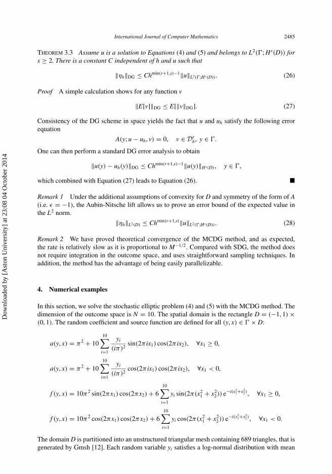
International Journal of Computer Mathematics 2487
−1−0.5
00.5
1
00.2
0.40.6
0.81
−0.2
−0.15
−0.1
−0.05
0
0.05
0.1
0.15
x
NIPG discontinuous, log-normal: MCDG solution with 10,000 simulations, penalty = 100.0
y
(a)
−1
−0.5
0
0.5
1
0
0.2
0.4
0.6
0.8
10
0.005
0.01
0.015
0.02
0.025
0.03
0.035
0.04
x
NIPG discontinuous, log-normal: variance of 10,000 simulations, penalty = 100.0
y
(b)
Figure 3. MCDG approximations with parameters ε = 1 and σe = 100 for all faces e: (a) expected value and (b)variance.
−1−0.5
00.5
1
00.2
0.40.6
0.81
−0.2
−0.15
−0.1
−0.05
0
0.05
0.1
0.15
x
SIPG discontinuous, log−normal: MCDG solution with 10,000 simulations, penalty = 1.0
y
(a)
−1−0.5
00.5
1
00.2
0.40.6
0.810
0.01
0.02
0.03
0.04
x
SIPG discontinuous, log-normal: variance of 10,000 simulations, penalty = 1.0
y
(b)
Figure 4. MCDG approximations with parameters ε = −1 and σe = 1 for all faces e: (a) expected value and (b) variance.
−1−0.5
00.5
1
00.2
0.40.6
0.81
−0.2
−0.15
−0.1
−0.05
0
0.05
0.1
0.15
x
SIPG discontinuous, log-normal: MCDG solution with 10,000 simulations, penalty = 10.0
y
(a)
−1−0.5
00.5
1
00.2
0.40.6
0.810
0.01
0.02
0.03
0.04
x
SIPG discontinuous, log-normal: variance of 10,000 simulations, penalty = 10.0
y
(b)
Figure 5. MCDG approximations with parameters ε = −1 and σe = 10 for all faces e: (a) expected value and (b)variance.
To further investigate the effect of the penalty values for the symmetric formulation, we repeatthe numerical experiments but we choose varying penalty values according to Equations (11) and(12). These equations show that the threshold penalty parameter value depends on the ratio of themaximum value of the coefficient a and its minimum value for all elements in the mesh. For agiven realization of a and a given mesh, the values of the penalty parameters vary across edges.We compute the maximum value and show in Figure 10(a) how this maximum value varies for
Dow
nloa
ded
by [
Ast
on U
nive
rsity
] at
23:
08 0
4 O
ctob
er 2
014
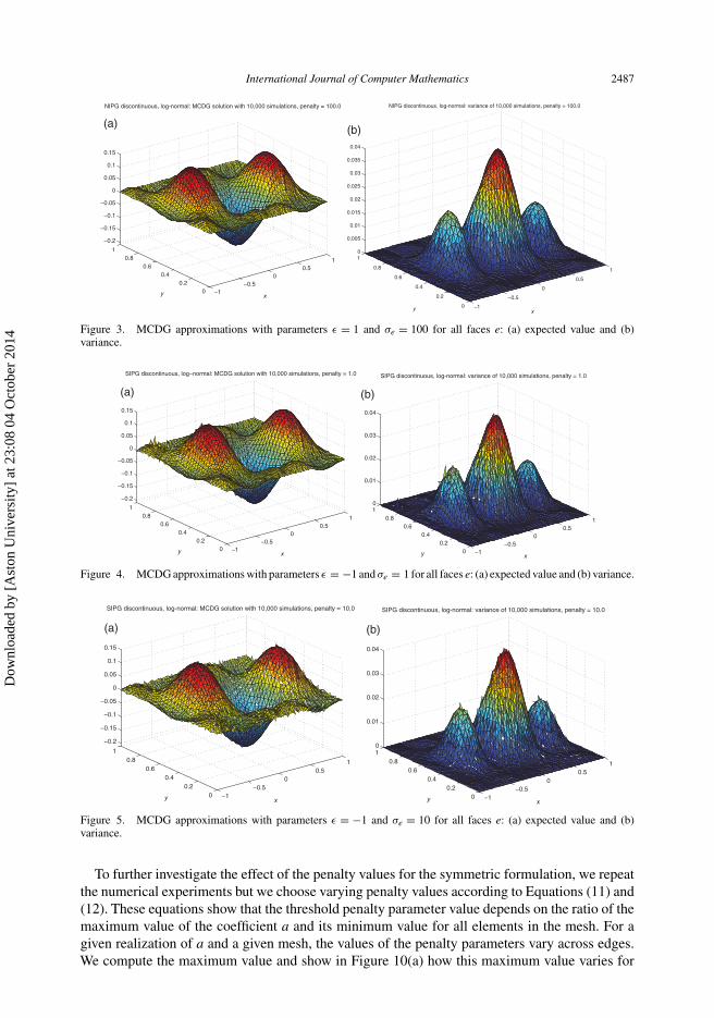
2488 K. Liu and B.M. Rivière
−1−0.5
00.5
1
00.2
0.40.6
0.81
−0.2
−0.15
−0.1
−0.05
0
0.05
0.1
0.15
x
SIPG discontinuous, log-normal: MCDG solution with 10,000 simulations, penalty = 100.0
y
(a)
−1−0.5
00.5
1
00.2
0.40.6
0.810
0.01
0.02
0.03
0.04
x
SIPG discontinuous, log-normal: variance of 10,000 simulations, penalty = 100.0
y
(b)
Figure 6. MCDG approximations with parameters ε = −1 and σe = 100 for all faces e: (a) expected value and (b)variance.
−1−0.5
00.5
1
00.2
0.40.6
0.81
−0.2
−0.15
−0.1
−0.05
0
0.05
0.1
0.15
x
IIPG discontinuous, log-normal: MCDG solution with 10,000 simulations, penalty = 1.0
y
(a)
−1−0.5
00.5
1
00.2
0.40.6
0.810
0.01
0.02
0.03
0.04
x
IIPG discontinuous, log-normal: variance of 10,000 simulations, penalty = 1.0
y
(b)
Figure 7. MCDG approximations with parameters ε = 0 and σe = 1 for all faces e: (a) expected value and (b) variance.
−1−0.5
0
1
00.2
0.40.6
0.81
−0.2
−0.15
−0.1
−0.05
0
0.05
0.1
0.15
x
IIPG discontinuous, log-normal: MCDG solution with 10,000 simulations, penalty = 10.0
y
(a)
−1−0.5
00.5
1
00.2
0.40.6
0.810
0.01
0.02
0.03
0.04
x
IIPG discontinuous, log-normal: variance of 10,000 simulations, penalty = 10.0
y
(b)
Figure 8. MCDG approximations with parameters ε = 0 and σe = 10 for all faces e: (a) expected value and (b) variance.
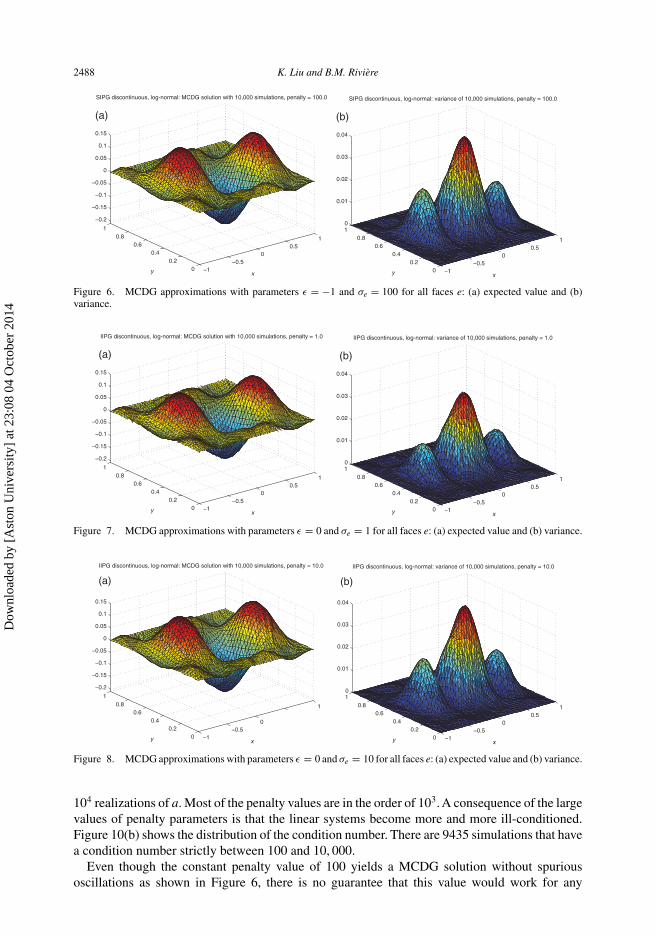
104 realizations of a. Most of the penalty values are in the order of 103. A consequence of the largevalues of penalty parameters is that the linear systems become more and more ill-conditioned.Figure 10(b) shows the distribution of the condition number. There are 9435 simulations that havea condition number strictly between 100 and 10, 000.
Even though the constant penalty value of 100 yields a MCDG solution without spuriousoscillations as shown in Figure 6, there is no guarantee that this value would work for any
Dow
nloa
ded
by [
Ast
on U
nive
rsity
] at
23:
08 0
4 O
ctob
er 2
014

International Journal of Computer Mathematics 2489
−1−0.5
00.5
1
00.2
0.40.6
0.81
−0.2
−0.15
−0.1
−0.05
0
0.05
0.1
0.15
x
IIPG discontinuous, log-normal: MCDG solution with 10,000 simulations, penalty = 100.0
y
(a)
−1−0.5
00.5
1
00.2
0.40.6
0.810
0.01
0.02
0.03
0.04
x
IIPG discontinuous, log-normal: variance of 10,000 simulations, penalty = 100.0
y
(b)
Figure 9. MCDG approximations with parameters ε = 0 and σe = 100 for all faces e: (a) expected value and (b)variance.
1000 1100 1200 1300 1400 1500 16000
50
100
150
200
250Distribution of penalty parameter, max = 1.51e+03, min = 1.06e+03
(a)
0 1000 2000 3000 4000 5000 6000 7000 8000 9000 100000
10
20
30
40
50
60
70
80
90
100Distribution of condition number: max = 9.7e+03, min = 100.9
(b)
Figure 10. Stable SIPG simulations: (a) penalty values and (b) condition number.
−1−0.5
00.5
1
00.2
0.40.6
0.81
−2
0
2
4
6
8
x 10−3
x
Difference of MCDG solution with contant and various penalty
y
(a)
−1−0.5
00.5
1
00.2
0.40.6
0.81
−15
−10
−5
0
5
x 10−4
x
Difference of variance of 10,000 simulations with contant and various penalty
y
(b)
Figure 11. Pointwise errors between MCDG solutions with constant penalty value and with varying penalty value.
stochastic coefficients. The use of varying penalty values according to Equations (11) and (12)would guarantee a stable solution. Figure 11 shows the pointwise differences between the MCDGsolution obtained with penalty equal to 100 and the MCDG solution obtained with varying penaltyvalues. In this numerical example, the maximum errors are 10% for the expected value and 3%for the variance.
Dow
nloa
ded
by [
Ast
on U
nive
rsity
] at
23:
08 0
4 O
ctob
er 2
014
2490 K. Liu and B.M. Rivière
5. Conclusions
We describe two approaches for solving elliptic problems with random coefficients: the first onehandles the uncertainty in a Galerkin framework, and the second one is based on the popularMonte Carlo technique. By utilizing locally mass conservative discontinuous Galerkin methods,our work is well suited to simulate flows in random porous media. This paper focuses on thetheoretical convergence of both approaches. The numerical results for the MCDG approach indi-cate that penalty values and solutions for the non-symmetric interior penalty Galerkin methodare independent of the variations of the stochastic coefficients. The symmetric and incompleteversions depend strongly to the magnitude of the penalty value, which in turn depends on thevariations of the stochastic coefficients. This yields linear systems with large condition numbers.
References
[1] M. Ainsworth and R. Rankin, Technical note: a note on the selection of the penalty parameter for discontinuousGalerkin finite element schemes, Numer. Methods Partial Differ. Equ. 28 (2012), pp. 1099–1104.
[2] D. Arnold, An interior penalty finite element method with discontinuous elements, SIAM J. Numer. Anal. 19 (1982),pp. 742–760.
[3] I. Babuska, F. Nobile, and R. Tempone, A stochastic collocation method for elliptic partial differential equationswith random input data, SIAM J. Numer. Anal. 45 (2007), pp. 1005–1034.
[4] I. Babuska, R. Tempone, and G. Zouraris, Galerkin finite element approximations of stochastic elliptic partialdifferential equations, SIAM J. Numer. Anal. 42 (2004), pp. 800–825.
[5] F. Benth and J. Gjerde, Convergence rates for finite element approximations of stochastic partial differentialequations, Stoch. Stoch. Rep. 63 (1998), pp. 313–326.
[6] P. Billingsley, Probability and Measure, Wiley, New York, 1995.[7] Y. Cao, K. Zhang, and R. Zhang, Finite element method and discontinuous Galerkin method for stochastic scattering
problem of Helmholtz type, Potential Anal. 28 (2008), pp. 301–319.[8] C. Dawson, S. Sun, and M. Wheeler, Compatible algorithms for coupled flow and transport, Comput. Methods Appl.
Mech. Eng. 193 (2004), pp. 2565–2580.[9] M. Deb, I. Babuska, and J. Oden, Solution of stochastic partial differential equations using Galerkin finite element
techniques, Comput. Methods Appl. Mech. Eng. 190 (2001), pp. 6539–6372.[10] Y. Epshteyn and B. Rivière, Estimation of penalty parameters for symmetric interior penalty Galerkin methods,
J. Comput. Appl. Math. 206 (2007), pp. 843–872. doi:10.1016/j.cam.2006.08.029.[11] P. Frauenfelder, C. Schwab, and R. Todor, Finite elements for elliptic problems with stochastic coefficients, Comput.
Methods Appl. Mech. Eng. 194 (2005), pp. 205–228.[12] C. Geuzaine and J.F. Remacle, Gmsh: a three-dimensional finite element mesh generator with built-in pre- and
post-processing facilities, Int. J. Numer. Methods Eng. 79 (2009), pp. 1309–1331. http://www.geuz.org/gmsh/[13] R. Ghanem and P. Spanos, Stochastic Finite Elements: A Spectral Approach, Springer, New York, 1991.[14] G. Karniadakis and D. Xiu, The Wiener–Askey polynomial chaos for stochastic differential equations, SIAM J. Sci.
Comput. 24 (2002), pp. 619–644.[15] M. Loève, Probability Theory, Springer-Verlag, Berlin, 1977.[16] H. Matthies andA. Keese, Galerkin methods for linear and nonlinear elliptic stochastic partial differential equations,
Comput. Methods Appl. Mech. Eng. 194 (2005), pp. 1295–1331.[17] F. Nobile, R. Tempone, and C. Webster, A sparse grid stochastic collocation method for partial differential equations
with random input data, SIAM J. Numer. Anal. 46 (2008), pp. 2309–2345.[18] B. Riviere, Discontinuous Galerkin Methods for Solving Elliptic and Parabolic Equations: Theory and Implemen-
tation, SIAM, Philadelphia, 2008.[19] B. Rivière, M. Wheeler, and K. Banas, Part II. Discontinuous Galerkin method applied to a single phase flow in
porous media, Comput. Geosci. 4 (2000), pp. 337–349.[20] B. Rivière, M. Wheeler, and V. Girault, A priori error estimates for finite element methods based on discontinuous
approximation spaces for elliptic problems, SIAM J. Numer. Anal. 39 (2001), pp. 902–931.[21] K. Shahbazi, An explicit expression for the penalty parameter of the interior penalty method, J. Comput. Phys.
205 (2005), pp. 401–407.[22] M. Wheeler, An elliptic collocation-finite element method with interior penalties, SIAM J. Numer. Anal. 15 (1978),
pp. 152–161.[23] D. Xiu and J. Hesthaven, High-order collocation methods for differential equations with random inputs, SIAM J.
Sci. Comput. 27 (2005), pp. 1118–1139.[24] R.M. Yao and L.J. Bo, Discontinuous Galerkin method for elliptic stochastic partial differential equations on two
and three dimensional spaces, Sci. China Ser. A: Math. 50 (2007), pp. 1661–1672.
Dow
nloa
ded
by [
Ast
on U
nive
rsity
] at
23:
08 0
4 O
ctob
er 2
014