disclaimer the stochastic topic block model - imag.fr · the stochastic topic block model charles...

The Stochastic Topic Block Model

Charles BOUVEYRON

Laboratoire MAP5, UMR CNRS 8145

Université Paris Descartes

[email protected]

up5.fr/bouveyron

Joint work with P. Latouche & R. Zreik

1

Disclaimer

“Essentially, all models are wrong but some are useful”

George E.P. Box

2

Outline

Introduction

The STBM model

Inference

Applications to an email network

Applications to a co-authorship network

Conclusion

3

Introduction

Statistical analysis of (social) networks has become a strong discipline:⌅ description and comparison of networks,⌅ network visualization,⌅ clustering of network nodes.

with applications in domains ranging from biology to historical sciences:⌅ biology: analysis of gene regulation processes,⌅ social sciences: analysis of political blogs,⌅ historical sciences: clustering and comparison of medieval social networks

⇤Bouveyron, Lamassé et al., The random subgraph model for the analysis of

an ecclesiastical network in merovingian Gaul, The Annals of Applied

Statistics, vol. 8(1), pp. 377-405, 2014.

4

Introduction

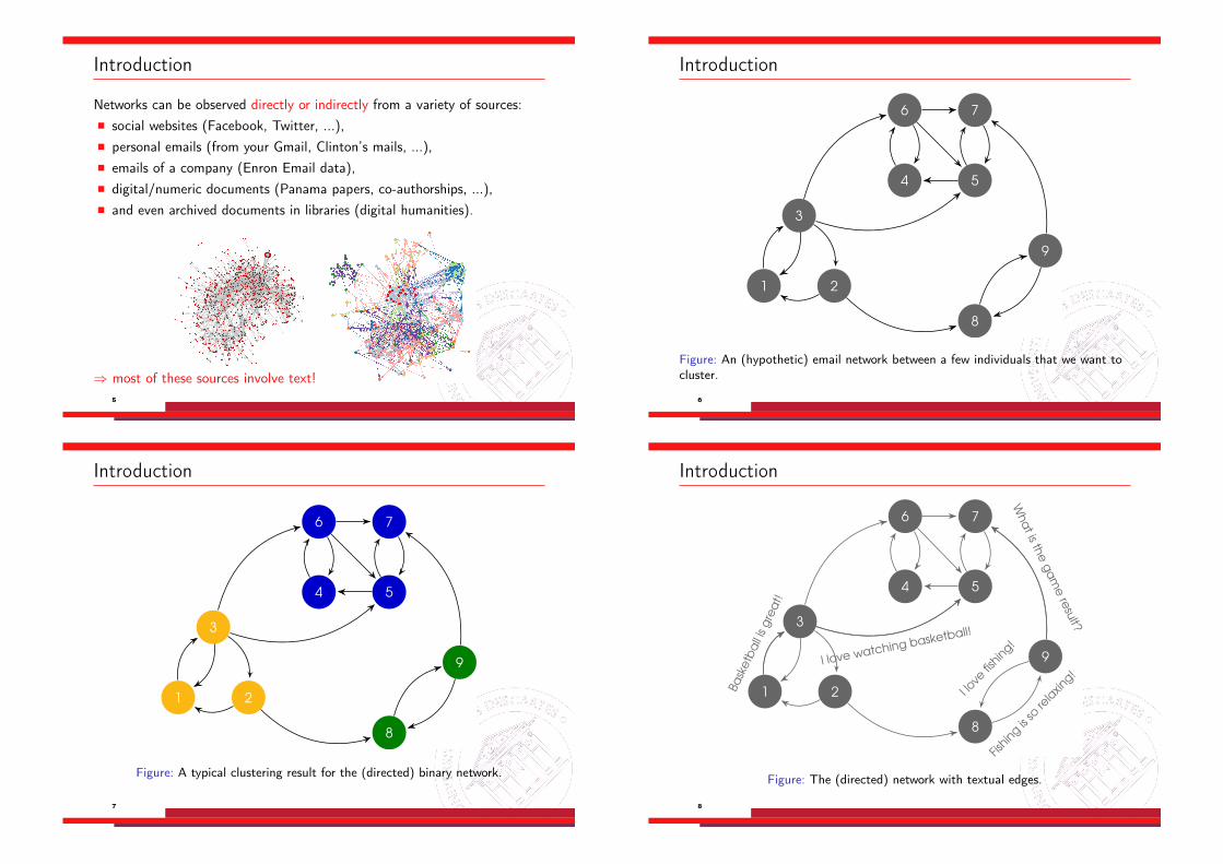
Networks can be observed directly or indirectly from a variety of sources:⌅ social websites (Facebook, Twitter, ...),⌅ personal emails (from your Gmail, Clinton’s mails, ...),⌅ emails of a company (Enron Email data),⌅ digital/numeric documents (Panama papers, co-authorships, ...),⌅ and even archived documents in libraries (digital humanities).

) most of these sources involve text!5

Introduction

1 2

3

4

6

5

7

8

9

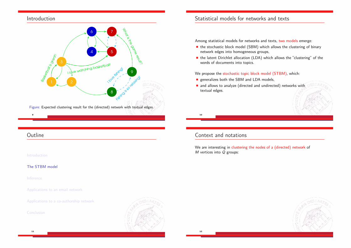
Figure: An (hypothetic) email network between a few individuals that we want to

cluster.

6

Introduction

1 2

3

4

6

5

7

8

9

Figure: A typical clustering result for the (directed) binary network.

7

Introduction

1 2

3

B

a

s

k

e

t

b

a

l

l

i

s

g

r

e

a

t

!

4

6

5

7

I

l

o

v

e

w

a

t

c

h

i

n

g

b

a

s

k

e

t

b

a

l

l

!

8

9

I

l

o

v

e

fi

s

h

i

n

g

!

F

i

s

h

i

n

g

i

s

s

o

r

e

l

a

x

i

n

g

!

W

h

a

t

i

s

t

h

e

g

a

m

e

r

e

s

u

l

t

?

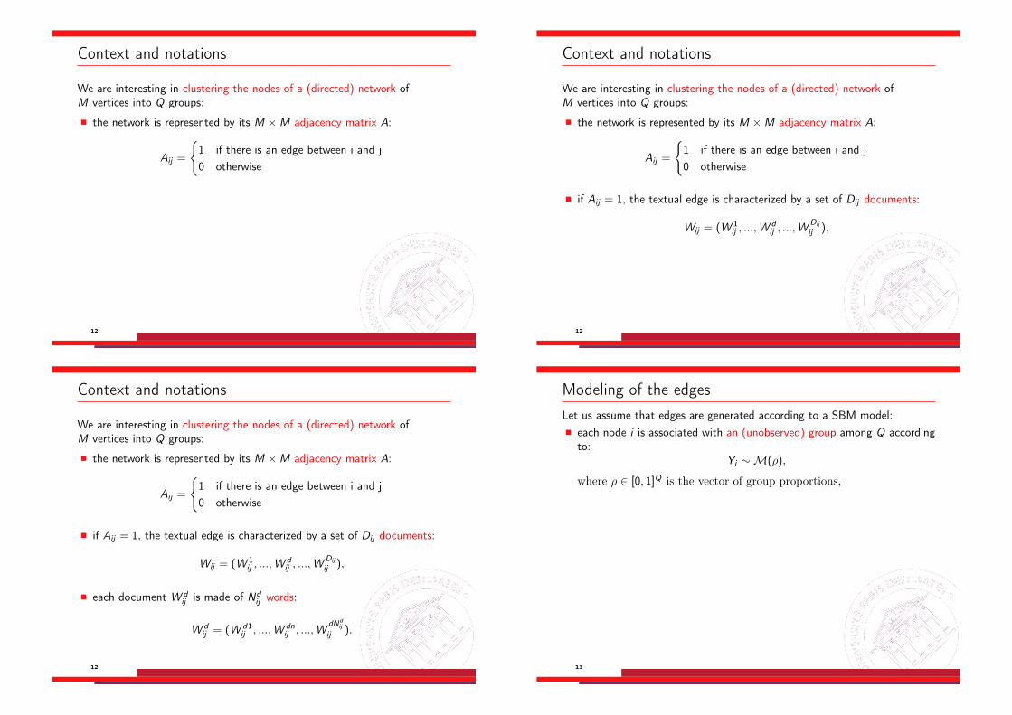
Figure: The (directed) network with textual edges.

8

Introduction

1 2

3

B

a

s

k

e

t

b

a

l

l

i

s

g

r

e

a

t

!

4

6

5

7

I

l

o

v

e

w

a

t

c

h

i

n

g

b

a

s

k

e

t

b

a

l

l

!

8

9

I

l

o

v

e

fi

s

h

i

n

g

!

F

i

s

h

i

n

g

i

s

s

o

r

e

l

a

x

i

n

g

!

W

h

a

t

i

s

t

h

e

g

a

m

e

r

e

s

u

l

t

?

Figure: Expected clustering result for the (directed) network with textual edges.

9

Statistical models for networks and texts

Among statistical models for networks and texts, two models emerge:⌅ the stochastic block model (SBM) which allows the clustering of binary

network edges into homogeneous groups,⌅ the latent Dirichlet allocation (LDA) which allows the ”clustering” of the

words of documents into topics.

We propose the stochastic topic block model (STBM), which:⌅ generalizes both the SBM and LDA models,⌅ and allows to analyze (directed and undirected) networks with

textual edges.

10

Outline

Introduction

The STBM model

Inference



Conclusion

11

Context and notations

We are interesting in clustering the nodes of a (directed) network ofM vertices into Q groups:

⌅ the network is represented by its M ⇥M adjacency matrix A:

Aij =

(1 if there is an edge between i and j0 otherwise

⌅ if Aij = 1, the textual edge is characterized by a set of Dij documents:

Wij = (W 1

ij , ...,Wdij , ...,W

Dij

ij ),

⌅ each document W dij is made of Nd

ij words:

W dij = (W d1

ij , ...,W dnij , ...,W

dNdij

ij ).

12




Aij =



Wij = (W 1

ij , ...,Wdij , ...,W

Dij

ij ),


ij words:

W dij = (W d1

ij , ...,W dnij , ...,W

dNdij

ij ).

12




Aij =



Wij = (W 1

ij , ...,Wdij , ...,W

Dij

ij ),


ij words:

W dij = (W d1

ij , ...,W dnij , ...,W

dNdij

ij ).

12




Aij =



Wij = (W 1

ij , ...,Wdij , ...,W

Dij

ij ),


ij words:

W dij = (W d1

ij , ...,W dnij , ...,W

dNdij

ij ).

12

Modeling of the edgesLet us assume that edges are generated according to a SBM model:⌅ each node i is associated with an (unobserved) group among Q according

to:Yi ⇠ M(⇢),

where ⇢ 2 [0, 1]Q is the vector of group proportions,

⌅ the presence of an edge Aij between i and j is drawn according to:

Aij |YiqYjr = 1 ⇠ B(⇡qr ),

where ⇡qr 2 [0, 1] is the connection probability between clusters q and r .

⌅ this leads to the following joint distribution:

p(A,Y |⇢,⇡) = p(A|Y ,⇡)p(Y |⇢)

=MY

i 6=j

QY

q,l

p(Aij |⇡qr )YiqYjr

MY

i=1

QY

q=1

⇢Yiqq .

13


to:Yi ⇠ M(⇢),






p(A,Y |⇢,⇡) = p(A|Y ,⇡)p(Y |⇢)

=MY

i 6=j

QY

q,l


MY

i=1

QY

q=1

⇢Yiqq .

13


to:Yi ⇠ M(⇢),






p(A,Y |⇢,⇡) = p(A|Y ,⇡)p(Y |⇢)

=MY

i 6=j

QY

q,l


MY

i=1

QY

q=1

⇢Yiqq .

13

Modeling of the documentsThe generative model for the documents is as follows:⌅ each pair of clusters (q, r) is first associated to a vector of topic

proportions ✓qr = (✓qrk)k sampled from a Dirichlet distribution:

✓qr ⇠ Dir (↵) ,

such thatPK

k=1

✓qrk = 1, 8(q, r).

⌅ the nth word W dnij of documents d in Wij is then associated to a latent

topic vector Z dnij according to:

Z dnij | {AijYiqYjr = 1, ✓} ⇠ M (1, ✓qr ) .

⌅ then, given Z dnij , the word W dn

ij is assumed to be drawn from amultinomial distribution:

W dnij |Z dnk

ij = 1 ⇠ M (1,�k = (�k1

, . . . ,�kV )) ,

where V is the vocabulary size.

14



✓qr ⇠ Dir (↵) ,

such thatPK

k=1

✓qrk = 1, 8(q, r).






W dnij |Z dnk

ij = 1 ⇠ M (1,�k = (�k1

, . . . ,�kV )) ,

where V is the vocabulary size.

14



✓qr ⇠ Dir (↵) ,

such thatPK

k=1

✓qrk = 1, 8(q, r).






W dnij |Z dnk

ij = 1 ⇠ M (1,�k = (�k1

, . . . ,�kV )) ,

where V is the vocabulary size.14

Modeling of the documents

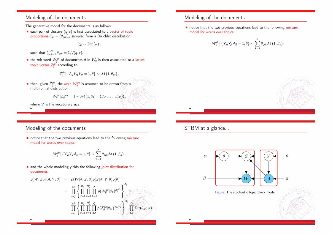
⌅ notice that the two previous equations lead to the following mixturemodel for words over topics:

W dnij | {YiqYjrAij = 1, ✓} ⇠

KX

k=1

✓qrkM (1,�k) .

⌅ and the whole modeling yields the following joint distribution fordocuments:

p(W ,Z , ✓|A,Y ,�) = p(W |A,Z ,�)p(Z |A,Y , ✓)p(✓)

=MY

i 6=j

8<

:

DijY

d=1

NdijY

n=1

KY

k=1

p(W dnij |�k)

Zdnkij

9=

;

Aij

⇥

MY

i 6=j

8<

:

DijY

d=1

NdijY

n=1

QY

q,r

p(Z dnij |✓qr )YiqYjr

9=

;

AijQY

q,r

Dir(✓qr ;↵).

15

Modeling of the documents

⌅ notice that the two previous equations lead to the following mixturemodel for words over topics:

W dnij | {YiqYjrAij = 1, ✓} ⇠

KX

k=1

✓qrkM (1,�k) .

⌅ and the whole modeling yields the following joint distribution fordocuments:

p(W ,Z , ✓|A,Y ,�) = p(W |A,Z ,�)p(Z |A,Y , ✓)p(✓)

=MY

i 6=j

8<

:

DijY

d=1

NdijY

n=1

KY

k=1

p(W dnij |�k)

Zdnkij

9=

;

Aij

⇥

MY

i 6=j

8<

:

DijY

d=1

NdijY

n=1

QY

q,r

p(Z dnij |✓qr )YiqYjr

9=

;

AijQY

q,r

Dir(✓qr ;↵).

15

STBM at a glance...

W

Z✓↵

� A

Y ⇢

⇡

Figure: The stochastic topic block model.

16

STBM at a glance...

1 2

3

⇡••, ✓••

4

6

5

7

⇡••, ✓••

8

9

⇡••, ✓••

⇡••, ✓••⇡••, ✓••

⇡••, ✓••

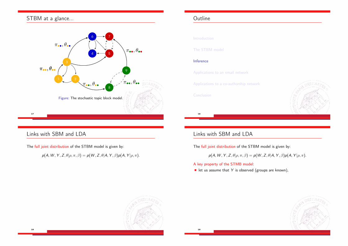
Figure: The stochastic topic block model.

17

Outline

Introduction

The STBM model

Inference



Conclusion

18

Links with SBM and LDA

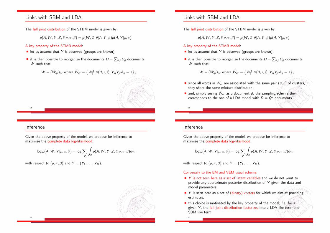
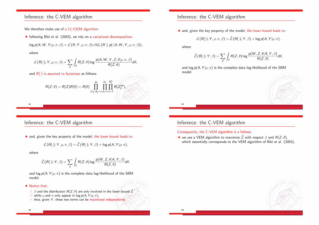
The full joint distribution of the STBM model is given by:

p(A,W ,Y ,Z , ✓|⇢,⇡,�) = p(W ,Z , ✓|A,Y ,�)p(A,Y |⇢,⇡).

A key property of the STMB model:⌅ let us assume that Y is observed (groups are known),

⌅ it is then possible to reorganize the documents D =P

i,j Dij documentsW such that:

W = (W̃qr )qr where W̃qr =�W d

ij , 8(d , i , j),YiqYjrAij = 1 ,

⌅ since all words in W̃qr are associated with the same pair (q, r) of clusters,they share the same mixture distribution,

⌅ and, simply seeing W̃qr as a document d , the sampling scheme thencorresponds to the one of a LDA model with D = Q2 documents.

19



p(A,W ,Y ,Z , ✓|⇢,⇡,�) = p(W ,Z , ✓|A,Y ,�)p(A,Y |⇢,⇡).








19



p(A,W ,Y ,Z , ✓|⇢,⇡,�) = p(W ,Z , ✓|A,Y ,�)p(A,Y |⇢,⇡).








19



p(A,W ,Y ,Z , ✓|⇢,⇡,�) = p(W ,Z , ✓|A,Y ,�)p(A,Y |⇢,⇡).








19

Inference

Given the above property of the model, we propose for inference tomaximize the complete data log-likelihood:

log p(A,W ,Y |⇢,⇡,�) = logX

Z

Z

✓p(A,W ,Y ,Z , ✓|⇢,⇡,�)d✓,

with respect to (⇢,⇡,�) and Y = (Y1

, . . . ,YM).

Conversely to the EM and VEM usual scheme:⌅ Y is not seen here as a set of latent variables and we do not want to

provide any approximate posterior distribution of Y given the data andmodel parameters,

⌅ Y is seen here as a set of (binary) vectors for which we aim at providingestimates,

⌅ this choice is motivated by the key property of the model, i.e. for agiven Y , the full joint distribution factorizes into a LDA like term andSBM like term.

20

Inference

Given the above property of the model, we propose for inference tomaximize the complete data log-likelihood:

log p(A,W ,Y |⇢,⇡,�) = logX

Z

Z

✓p(A,W ,Y ,Z , ✓|⇢,⇡,�)d✓,

with respect to (⇢,⇡,�) and Y = (Y1

, . . . ,YM).

Conversely to the EM and VEM usual scheme:⌅ Y is not seen here as a set of latent variables and we do not want to

provide any approximate posterior distribution of Y given the data andmodel parameters,

⌅ Y is seen here as a set of (binary) vectors for which we aim at providingestimates,

⌅ this choice is motivated by the key property of the model, i.e. for agiven Y , the full joint distribution factorizes into a LDA like term andSBM like term.20

Inference: the C-VEM algorithm

We therefore make use of a C(-V)EM algorithm:

⌅ following Blei et al. (2003), we rely on a variational decomposition:

log p(A,W ,Y |⇢,⇡,�) = L (R ;Y , ⇢,⇡,�)+KL (R k p(·|A,W ,Y , ⇢,⇡,�)) ,

where

L (R(·);Y , ⇢,⇡,�) =X

Z

Z

✓R(Z , ✓) log

p(A,W ,Y ,Z , ✓|⇢,⇡,�)R(Z , ✓)

d✓,

and R(·) is assumed to factorizes as follows:

R(Z , ✓) = R(Z )R(✓) = R(✓)MY

i 6=j,Aij=1

DijY

d=1

NdijY

n=1

R(Z dnij ).

21


⌅ and, given the key property of the model, the lower bound leads to:

L (R(·);Y , ⇢,⇡,�) = L̃ (R(·);Y ,�) + log p(A,Y |⇢,⇡),

where

L̃ (R(·);Y ,�) =X

Z

Z

✓R(Z , ✓) log

p(W ,Z , ✓|A,Y ,�)

R(Z , ✓)d✓,

and log p(A,Y |⇢,⇡) is the complete data log-likelihood of the SBMmodel.

⌅ Notice that:⇤ � and the distribution R(Z , ✓) are only involved in the lower bound L̃⇤

while ⇢ and ⇡ only appear in log p(A,Y |⇢,⇡),⇤

thus, given Y , these two terms can be maximized independently.

22


⌅ and, given the key property of the model, the lower bound leads to:

L (R(·);Y , ⇢,⇡,�) = L̃ (R(·);Y ,�) + log p(A,Y |⇢,⇡),

where

L̃ (R(·);Y ,�) =X

Z

Z

✓R(Z , ✓) log

p(W ,Z , ✓|A,Y ,�)

R(Z , ✓)d✓,

and log p(A,Y |⇢,⇡) is the complete data log-likelihood of the SBMmodel.

⌅ Notice that:⇤ � and the distribution R(Z , ✓) are only involved in the lower bound L̃⇤

while ⇢ and ⇡ only appear in log p(A,Y |⇢,⇡),⇤

thus, given Y , these two terms can be maximized independently.

22


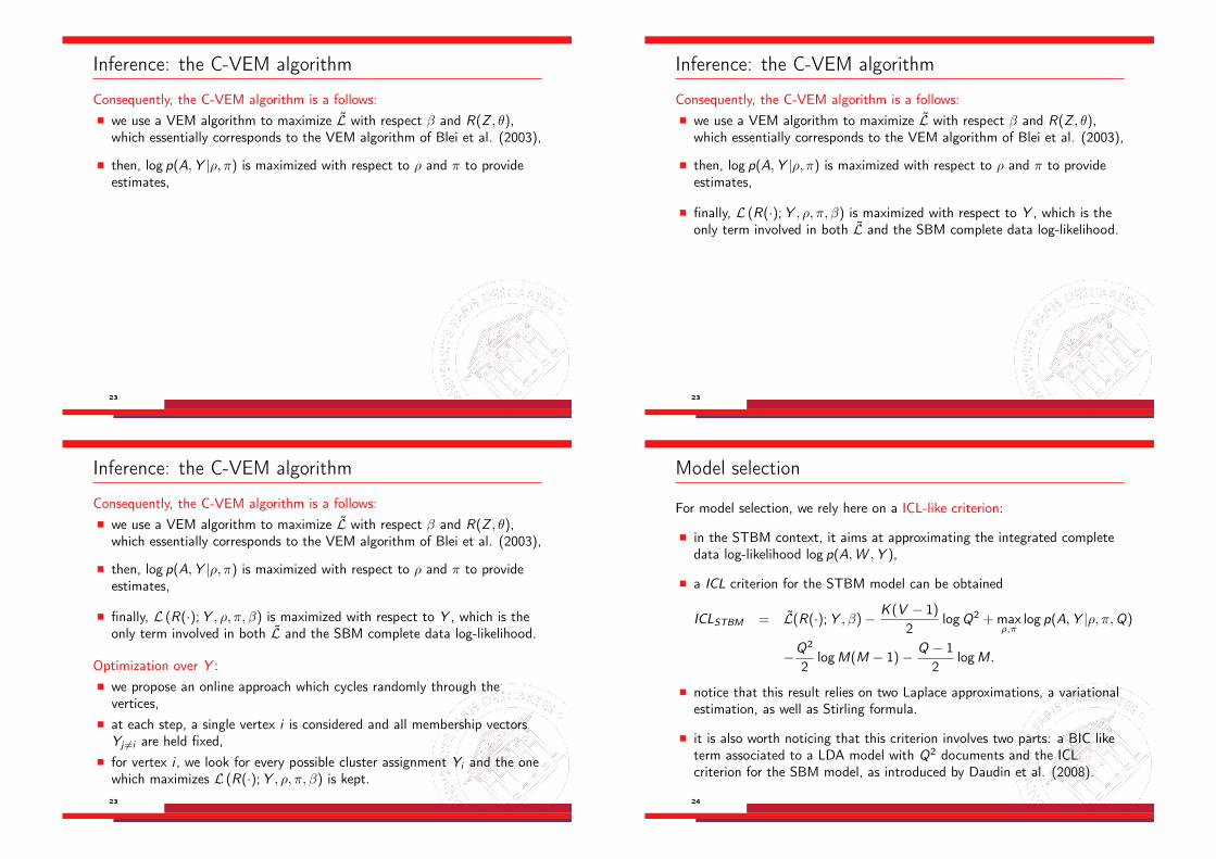
Consequently, the C-VEM algorithm is a follows:⌅ we use a VEM algorithm to maximize L̃ with respect � and R(Z , ✓),

which essentially corresponds to the VEM algorithm of Blei et al. (2003),

⌅ then, log p(A,Y |⇢,⇡) is maximized with respect to ⇢ and ⇡ to provideestimates,

⌅ finally, L (R(·);Y , ⇢,⇡,�) is maximized with respect to Y , which is theonly term involved in both L̃ and the SBM complete data log-likelihood.

Optimization over Y :⌅ we propose an online approach which cycles randomly through the

vertices,⌅ at each step, a single vertex i is considered and all membership vectors

Yj 6=i are held fixed,⌅ for vertex i , we look for every possible cluster assignment Yi and the one

which maximizes L (R(·);Y , ⇢,⇡,�) is kept.

23










23










23









which maximizes L (R(·);Y , ⇢,⇡,�) is kept.23

Model selection

For model selection, we rely here on a ICL-like criterion:

⌅ in the STBM context, it aims at approximating the integrated completedata log-likelihood log p(A,W ,Y ),

⌅ a ICL criterion for the STBM model can be obtained

ICLSTBM = L̃(R(·);Y ,�)� K (V � 1)2

logQ2 + max⇢,⇡

log p(A,Y |⇢,⇡,Q)

�Q2

2logM(M � 1)� Q � 1

2logM.

⌅ notice that this result relies on two Laplace approximations, a variationalestimation, as well as Stirling formula.

⌅ it is also worth noticing that this criterion involves two parts: a BIC liketerm associated to a LDA model with Q2 documents and the ICLcriterion for the SBM model, as introduced by Daudin et al. (2008).

24

Outline

Introduction

The STBM model

Inference



Conclusion

25

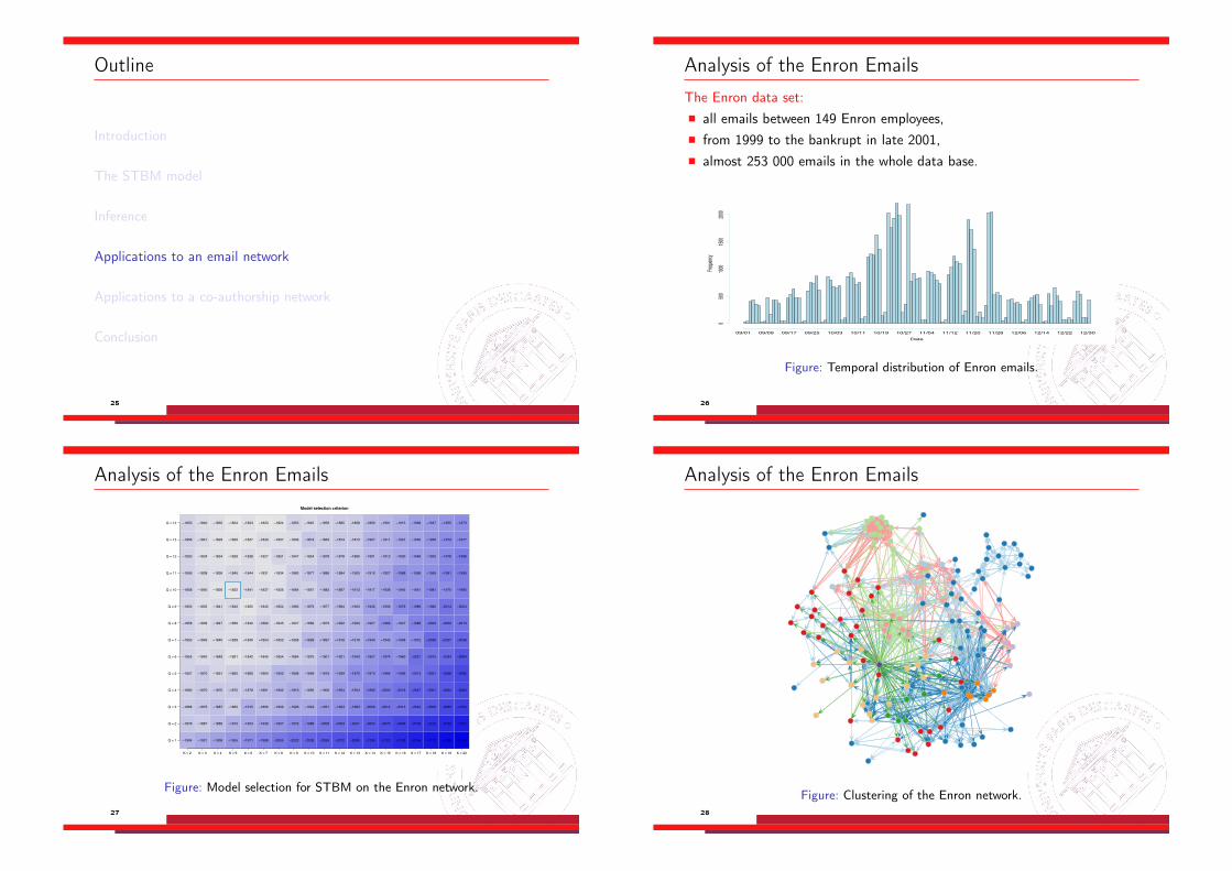
Analysis of the Enron EmailsThe Enron data set:⌅ all emails between 149 Enron employees,⌅ from 1999 to the bankrupt in late 2001,⌅ almost 253 000 emails in the whole data base.

Date

Freque

ncy

0500

1000

1500

2000

09/01 09/09 09/17 09/25 10/03 10/11 10/19 10/27 11/04 11/12 11/20 11/28 12/06 12/14 12/22 12/30

Figure: Temporal distribution of Enron emails.

26

Analysis of the Enron EmailsModel selection criterion

K = 2 K = 3 K = 4 K = 5 K = 6 K = 7 K = 8 K = 9 K = 10 K = 11 K = 12 K = 13 K = 14 K = 15 K = 16 K = 17 K = 18 K = 19 K = 20

Q = 1

Q = 2

Q = 3

Q = 4

Q = 5

Q = 6

Q = 7

Q = 8

Q = 9

Q = 10

Q = 11

Q = 12

Q = 13

Q = 14

−1904 −1921 −1938 −1955 −1971 −1988 −2005 −2022 −2038 −2055 −2072 −2089 −2106 −2122 −2139 −2156 −2173 −2189 −2206

−1876 −1867 −1889 −1912 −1924 −1939 −1957 −1975 −1989 −2009 −2023 −2041 −2054 −2075 −2092 −2106 −2122 −2139 −2157

−1868 −1876 −1887 −1865 −1915 −1895 −1909 −1926 −1924 −1951 −1964 −1983 −2006 −2014 −2013 −2044 −2062 −2089 −2104

−1860 −1870 −1870 −1870 −1878 −1891 −1902 −1919 −1895 −1906 −1954 −1954 −1992 −2003 −2018 −2047 −2051 −2064 −2084

−1857 −1870 −1851 −1860 −1866 −1864 −1902 −1898 −1899 −1919 −1939 −1970 −1970 −1984 −1996 −2013 −2031 −2068 −2085

−1855 −1842 −1849 −1831 −1842 −1845 −1854 −1864 −1875 −1901 −1921 −1943 −1957 −1974 −1960 −2021 −2015 −2034 −2064

−1853 −1846 −1840 −1838 −1840 −1854 −1853 −1858 −1899 −1897 −1916 −1918 −1944 −1945 −1958 −1972 −2030 −2027 −2038

−1858 −1839 −1847 −1836 −1842 −1862 −1845 −1847 −1869 −1873 −1902 −1909 −1927 −1966 −1947 −1988 −2003 −2009 −2013

−1852 −1835 −1841 −1843 −1825 −1845 −1854 −1863 −1879 −1877 −1894 −1903 −1940 −1936 −1976 −1986 −1982 −2014 −2004

−1858 −1840 −1826 −1822 −1841 −1837 −1835 −1864 −1857 −1883 −1897 −1912 −1917 −1938 −1945 −1951 −1981 −1975 −1995

−1856 −1838 −1836 −1845 −1844 −1831 −1834 −1863 −1877 −1886 −1884 −1900 −1910 −1927 −1968 −1958 −1969 −1991 −1995

−1853 −1834 −1834 −1828 −1838 −1827 −1851 −1847 −1854 −1879 −1878 −1880 −1901 −1912 −1930 −1948 −1955 −1978 −1998

−1856 −1841 −1829 −1826 −1827 −1840 −1837 −1839 −1874 −1863 −1874 −1873 −1907 −1911 −1931 −1935 −1956 −1973 −1977

−1853 −1840 −1835 −1824 −1834 −1823 −1824 −1855 −1845 −1859 −1865 −1868 −1893 −1901 −1915 −1938 −1947 −1955 −1973

Figure: Model selection for STBM on the Enron network.

27

Analysis of the Enron Emails

Fina

l clu

ster

ing

● ● ● ● ● ● ● ●

● ●

Gro

up 1

Gro

up 2

Gro

up 3

Gro

up 4

Gro

up 5

Gro

up 6

Gro

up 7

Gro

up 8

Gro

up 9

Gro

up 1

0

Topi

c 1

Topi

c 2

Topi

c 3

Topi

c 4

Topi

c 5

Figure: Clustering of the Enron network.

28

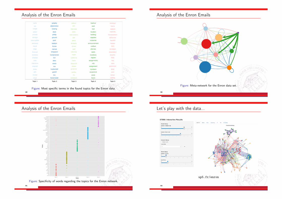
Analysis of the Enron EmailsTopics

Topic 1 Topic 2 Topic 3 Topic 4 Topic 5

clock heizenrader contracts floors netting

receipt bin rto aside kilmer

gas gaskill steffes equipment juanlimits kuykendall governor numbers pkgs

elapsed ina phase assignment geacconeinjections ermis dasovich rely sara

nom allen mara assignments kaywheeler tori california regular lindywindows fundamental super locations donoho

forecast sheppard saturday seats shackleton

ridge named said phones socalgas

equal forces dinner notified lynndeclared taleban fantastic announcement master

interruptible park davis computer hayslett

storage ground dwr supplies deliveries

prorata phillip interviewers building transwestern

select desk state location capacity

usage viewing interview test watson

ofo afghanistan puc seat harris

cycle grigsby edison backup mmbtud

Figure: Most specific terms in the found topics for the Enron data.

29


Figure: Meta-network for the Enron data set.

30


●●●●●●●●●

●●

●

●

●

●

●

●

●

●

●

●

●

●

●

●

●

●

●

●

●

●

●

●

●

●

●

●

●

●

●

●

●

●

●

●

●

●

●

●

●

●

●

●

●

●

●

●

●

●

●●●●●●●●●●

●

●

●

●

●

●

●

●

●

●

●

●

●

●

●

●

●

●

●

●

●

●

●

●

●

●

●

●

●

●

●

●

●

●

●

●

●

●

●

●

●

●

●

●

●

●

●

●

●

●●●●●●●●●●

●

●

●

●

●

●

●

●

●

●

●

●

●

●

●

●

●

●

●

●

●

●

●

●

●

●

●

●

●

●

●

●

●

●

●

●

●

●

●

●

●

●

●

●

●

●

●

●

●

●●●●●●●●●●

●

●

●

●

●

●

●

●

●

●

●

●

●

●

●

●

●

●

●

●

●

●

●

●

●

●

●

●

●

●

●

●

●

●

●

●

●

●

●

●

●

●

●

●

●

●

●

●

●

●●●●●●●●●

cycleofo

usagegas

storageselect

dayprorata

dailydeclared

grigsbydesk

phillipafghanistan

viewingnamed

allenpark

groundtalebanedison

pucinterview

statedavissaiddwr

californiainterviewers

contractsbackup

seattest

locationbuildingsupplies

planannouncement

computernotified

mmbtudcapacitywatson

harrisdeliveries

masteragreement

transwesternhayslett

Topic 1 Topic 2 Topic 3 Topic 4 Topic 5Topics

Wor

ds

Figure: Specificity of words regarding the topics for the Enron network.

31

Let’s play with the data...

up5.fr/enron

32

Outline

Introduction

The STBM model

Inference



Conclusion

33

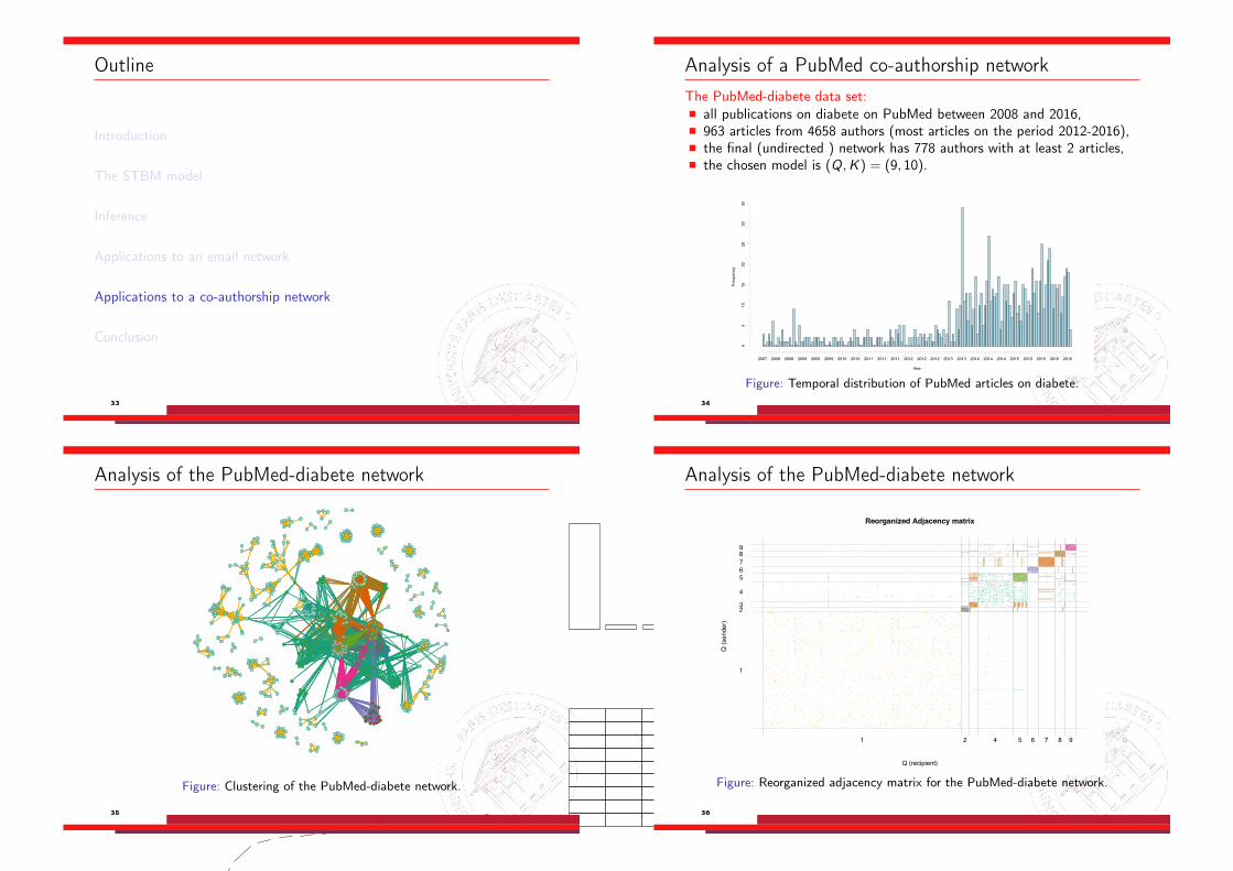
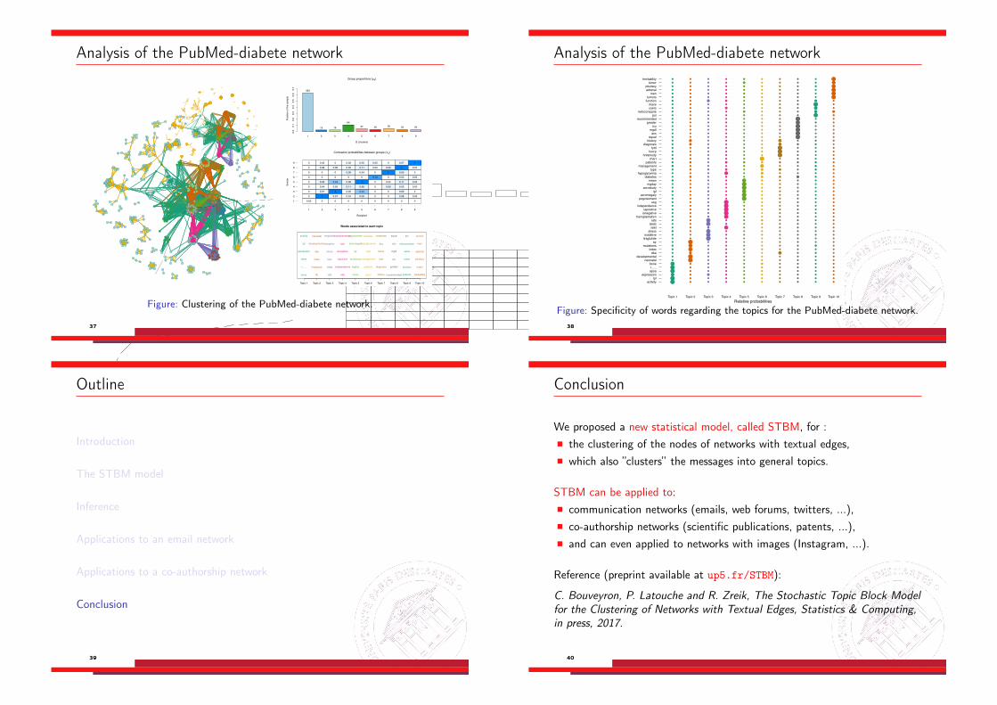
Analysis of a PubMed co-authorship networkThe PubMed-diabete data set:⌅ all publications on diabete on PubMed between 2008 and 2016,⌅ 963 articles from 4658 authors (most articles on the period 2012-2016),⌅ the final (undirected ) network has 778 authors with at least 2 articles,⌅ the chosen model is (Q,K ) = (9, 10).

Year

Frequency

05

1015

2025

3035

2007 2008 2008 2009 2009 2009 2010 2010 2011 2011 2011 2012 2012 2012 2013 2013 2014 2014 2014 2015 2015 2015 2016 2016

Figure: Temporal distribution of PubMed articles on diabete.

34

Analysis of the PubMed-diabete networkFinal clustering

●

●

●

●

●

● ●●

●●

●● ● ● ●

●

5 10 15

−760

0000

−740

0000

−720

0000

−700

0000

−680

0000

−660

0000

Lower−Bound

Iterations

Valu

e of

the

Lowe

r−Bo

und

Group proportions (ρq)

Q (clusters)

Frac

tion

of th

e sa

mpl

e

0.0

0.1

0.2

0.3

0.4

0.5

0.6

0.7

363

15 16

6427 20 30 20 20

1 2 3 4 5 6 7 8 9

Connexion probabilities between groups (πq)

Recipient

Send

er

0.02 0 0 0 0 0 0 0 0

0 1 0.07 0.04 0.09 0 0 0.08 0.02

0 0.07 1 0.05 0.44 0 0 0.06 0

0 0.04 0.05 0.11 0.08 0 0.09 0.05 0.02

0 0.09 0.44 0.08 1 0 0.04 0.11 0.05

0 0 0 0 0 0.74 0 0.03 0.05

0 0 0 0.09 0.04 0 1 0.09 0

0 0.08 0.06 0.05 0.11 0.03 0.09 1 0.07

0 0.02 0 0.02 0.05 0.05 0 0.07 1

1 2 3 4 5 6 7 8 9

1

2

3

4

5

6

7

8

9

Topic 1 Topic 2 Topic 3 Topic 4 Topic 5 Topic 6 Topic 7 Topic 8 Topic 9 Topic 10

Words associated to each topic

activity

lpl

expression

apoa

r......

bone

neonatal

developmental

dka

index

mutations

iqr

liraglutide

oxidative

stress

islet

islets

rats

transplantation

islet

ianegative

iapositive

independence

ukg

pegvisomant

acromegaly

igf

acrostudy

mgday

mean

diabetes

hypoglycemia

type

management

patients

chart

hnfamody

dka

hscrp

fytd

diagnosis

history

equal

acs

mgdl

icu

greater

recommended

poi

ketoconazole

users

mace

function

patients

tumors

men

adrenal

pituitary

tumor

heritability

Figure: Clustering of the PubMed-diabete network.

35

Analysis of the PubMed-diabete network

Reorganized Adjacency matrix

Q (recipient)

Q (s

ende

r)

1

23

4

56789

1 2 4 5 6 7 8 9

Figure: Reorganized adjacency matrix for the PubMed-diabete network.

36


Final clustering

●

●

●

●

●

● ●●

●●

●● ● ● ●

●

5 10 15

−760

0000

−740

0000

−720

0000

−700

0000

−680

0000

−660

0000

Lower−Bound

Iterations

Valu

e of

the

Lowe

r−Bo

und


Q (clusters)

Frac

tion

of th

e sa

mpl

e

0.0

0.1

0.2

0.3

0.4

0.5

0.6

0.7

363

15 16

6427 20 30 20 20

1 2 3 4 5 6 7 8 9


Recipient

Send

er0.02 0 0 0 0 0 0 0 0

0 1 0.07 0.04 0.09 0 0 0.08 0.02

0 0.07 1 0.05 0.44 0 0 0.06 0

0 0.04 0.05 0.11 0.08 0 0.09 0.05 0.02

0 0.09 0.44 0.08 1 0 0.04 0.11 0.05

0 0 0 0 0 0.74 0 0.03 0.05

0 0 0 0.09 0.04 0 1 0.09 0

0 0.08 0.06 0.05 0.11 0.03 0.09 1 0.07

0 0.02 0 0.02 0.05 0.05 0 0.07 1

1 2 3 4 5 6 7 8 9

1

2

3

4

5

6

7

8

9



activity

lpl

expression

apoa

r......

bone

neonatal

developmental

dka

index

mutations

iqr

liraglutide

oxidative

stress

islet

islets

rats

transplantation

islet

ianegative

iapositive

independence

ukg

pegvisomant

acromegaly

igf

acrostudy

mgday

mean

diabetes

hypoglycemia

type

management

patients

chart

hnfamody

dka

hscrp

fytd

diagnosis

history

equal

acs

mgdl

icu

greater

recommended

poi

ketoconazole

users

mace

function

patients

tumors

men

adrenal

pituitary

tumor

heritability

Final clustering

●

●

●

●

●

● ●●

●●

●● ● ● ●

●

5 10 15

−760

0000

−740

0000

−720

0000

−700

0000

−680

0000

−660

0000

Lower−Bound

Iterations

Valu

e of

the

Lowe

r−Bo

und


Q (clusters)

Frac

tion

of th

e sa

mpl

e

0.0

0.1

0.2

0.3

0.4

0.5

0.6

0.7

363

15 16

6427 20 30 20 20

1 2 3 4 5 6 7 8 9


Recipient

Send

er

0.02 0 0 0 0 0 0 0 0

0 1 0.07 0.04 0.09 0 0 0.08 0.02

0 0.07 1 0.05 0.44 0 0 0.06 0

0 0.04 0.05 0.11 0.08 0 0.09 0.05 0.02

0 0.09 0.44 0.08 1 0 0.04 0.11 0.05

0 0 0 0 0 0.74 0 0.03 0.05

0 0 0 0.09 0.04 0 1 0.09 0

0 0.08 0.06 0.05 0.11 0.03 0.09 1 0.07

0 0.02 0 0.02 0.05 0.05 0 0.07 1

1 2 3 4 5 6 7 8 9

1

2

3

4

5

6

7

8

9



activity

lpl

expression

apoa

r......

bone

neonatal

developmental

dka

index

mutations

iqr

liraglutide

oxidative

stress

islet

islets

rats

transplantation

islet

ianegative

iapositive

independence

ukg

pegvisomant

acromegaly

igf

acrostudy

mgday

mean

diabetes

hypoglycemia

type

management

patients

chart

hnfamody

dka

hscrp

fytd

diagnosis

history

equal

acs

mgdl

icu

greater

recommended

poi

ketoconazole

users

mace

function

patients

tumors

men

adrenal

pituitary

tumor

heritability

Figure: Clustering of the PubMed-diabete network.

37


●●●●●●●●

●

●

●

●

●

●

●

●

●

●

●

●

●

●

●

●

●

●

●

●

●

●

●

●

●

●

●

●

●

●

●

●

●

●

●

●

●

●

●

●

●

●

●

●

●

●

●

●

●

●

●

●

●

●

●

●

●●●●●●

●

●

●

●

●

●

●

●

●

●

●

●

●

●

●

●

●

●

●

●

●

●

●

●

●

●

●

●

●

●

●

●

●

●

●

●

●

●

●

●

●

●

●

●

●

●

●

●

●

●

●

●

●

●

●

●

●

●●●●

●●●

●

●

●

●

●

●

●

●

●

●

●

●

●

●

●

●

●

●

●

●

●

●

●

●

●

●

●

●

●

●

●

●

●

●

●

●

●

●

●

●

●

●

●

●

●

●

●

●

●

●

●

●

●

●●

●

●●●●●

●

●

●

●

●

●

●

●●

●

●

●

●

●

●

●

●

●

●

●

●

●

●

●

●

●

●

●

●

●

●

●

●

●

●

●

●

●

●

●

●

●

●

●

●

●

●

●

●

●

●

●

●

●

●

●

●

●●●●●●●

●

●

●

●

●

●

●

●

●

●

●

●

●

●

●

●

●

●

●

●

●

●

●

●

●

●

●

●

●

●

●

●

●

●

●

●

●

●

●

●

●

●

●

●

●

●

●

●

●

●

●

●

●

●

●

●

●

●

●

●●

●●

●

●

●

●

●

●

●

●

●

●

●

●

●

●

●

●

●

●

●

●

●

●

●

●

●

●

●

●

●

●

●

●

●

●

●

●

●

●

●

●

●

●

●

●

●

●

●

●

●

●

●

●

●

●

●

●

●●●●●

●

●

●

●

●

●

●

●

●

●

●

●

●

●

●

●

●

●

●

●

●

●

●

●

●

●

●

●

●

●

●

●

●

●

●

●

●

●

●

●

●

●

●

●

●

●

●

●

●

●

●

●

●

●

●

●

●

●●●●●●

●

●

●

●

●

●

●

●

●

●

●

●

●

●

●

●

●

●

●

●

●

●

●

●

●

●

●

●

●

●

●

●

●

●

●

●

●

●

●

●

●

●

●

●

●

●

●

●

●

●

●

●

●

●

●

●

●

●●●●●

●

●

●

●

●

●

●

●

●

●

●

●

●

●

●

●

●

●

●

●

●

●

●

●

●

●

●

●

●

●

●

●

●

●

●

●

●

●

●

●

●

●

●

●

●

●

●

●

●

●

●

●

●

●

●

●

●

●●●●●●


activitylpl

expressionapoar......bone

neonataldevelopmental

dkaindex

mutationsiqr

liraglutideoxidative

stressislet

isletsrats

transplantationianegativeiapositive

independenceukg

pegvisomantacromegaly

igfacrostudy

mgdaymean

diabeteshypoglycemia

typemanagement

patientschart

hnfamodyhscrp

fytddiagnosis

historyequal

acsmgdl

icugreater

recommendedpoi

ketoconazoleusersmace

functiontumors

menadrenalpituitary

tumorheritability

Relative probabilities

Figure: Specificity of words regarding the topics for the PubMed-diabete network.

38

Outline

Introduction

The STBM model

Inference



Conclusion

39

Conclusion

We proposed a new statistical model, called STBM, for :⌅ the clustering of the nodes of networks with textual edges,⌅ which also ”clusters” the messages into general topics.

STBM can be applied to:⌅ communication networks (emails, web forums, twitters, ...),⌅ co-authorship networks (scientific publications, patents, ...),⌅ and can even applied to networks with images (Instagram, ...).

Reference (preprint available at up5.fr/STBM):

C. Bouveyron, P. Latouche and R. Zreik, The Stochastic Topic Block Model

for the Clustering of Networks with Textual Edges, Statistics & Computing,

in press, 2017.

40

Announcement: Statlearn’17, April, 5-7, 2017, Lyon

Program and registration at http://statlearn.sfds.asso.fr.

41

disclaimer the stochastic topic block model - imag.fr · the stochastic topic block model charles...

Documents