direction of change prediction in the eur/usd … fileeur/usd exchange rate volatility using neural...

İSTANBUL BİLGİ UNIVERSITY

INSTITUTE OF SOCIAL SCIENCES

DIRECTION OF CHANGE PREDICTION IN THE

EUR/USD EXCHANGE RATE VOLATILITY USING

NEURAL NETWORK MODELS

Mustafa SIR

İstanbul June 2010

İSTANBUL BİLGİ UNIVERSITY

INSTITUTE OF SOCIAL SCIENCES

DIRECTION OF CHANGE PREDICTION IN THE EUR/USD

EXCHANGE RATE VOLATILITY USING FEED FORWARD

NEURAL NETWORK MODEL

Submitted by Mustafa SIR

In the Partial Fulfillment of the Requirements for the Degree of

Master of Science in Name of the Discipline June 2010

Approved by:

Orhan ERDEM Orhan ERDEM Head of Department Dissertation Supervisor

DIRECTION OF CHANGE PREDICTION IN THE EUR/USD

EXCHANGE RATE VOLATILITY USING NEURAL

NETWORK MODELS

Mustafa SIR 107624001

Ass. Prof. Dr. Orhan ERDEM : .......................................... Asc. Prof. Dr. Ege YAZGAN : .......................................... Asc. Prof. Dr. Kerem ŞENEL : ..........................................

Tezin Onaylandığı Tarih :22.06.2010

Toplam Sayfa Sayısı :69 Anahtar Kelimeler (Türkçe) Anahtar Kelimeler (İngilizce) 1) Yapay Sinir Ağları 1) Artificial Neural Networks 2) Oynaklık Modellemesi 2) Volatility Modeling 3) EUR/USD Döviz Kuru 3) EUR/USD Exchange Rate

iv

Abstract

The aim of this thesis is to examine the forecastability of various volatility

proxies for EUR/USD exchange rate by the means of a Feed Forward

Neural Network Model. Analyzed volatility proxies consist of two groups,

namely low frequency proxies and proxies obtained from high frequency

intraday data. After distributional properties and the characteristics of the

proxies such as persistency, mean reversion and asymmetry are analyzed,

the direction of change in the level of the series for the next day are

predicted with a three layered Feed Forward Neural Network Model.

The first conclusion of the thesis is that the predictability of low frequency

volatility proxies are higher than that of high frequency based proxies. On

the other hand, when they are normalized with daily returns, high frequency

based proxies become more predictable than un normalized high frequency

based proxies.

The second conclusion of the thesis is that high frequency based proxies

become normally distributed when they are normalized with daily returns.

These normalized series, unlike from un-normalized ones, do not display the

stylized facts of volatility. However, their predictability is found to be

superior, leading to an inference that the distributional property may have a

stronger effect on predictability than the stylized facts do.

v

Özet

Bu tezin amacı, EUR/USD paritesindeki oynaklığı modelleyen zaman

serileri geliştirmek ve bu serilerin tahmin edilebilirliğini İleri Beslemeli

Yapay Sinir Ağları ile incelemektir. İncelenen oynaklık göstergeleri, düşük

frekanslı olanlar ve gün içi yüksek frekanslı verilerden elde edilenler olmak

üzere iki gruba ayrılmıştır. Gösterge serilerin dağılımsal nitelikleri ile

kalıcılık, ortalamaya yakınsama ve asimetriklik gibi karakteristik özellikleri

irdelendikten sonra seviyelerdeki değişimin yönü üç katmanlı İleri

Beslemeli Sinir Ağı Modeli ile tahmin edilmeye çalışılmıştır.

Çalışmada elde edilen bulgulardan ilki, düşük frekanslı oynaklık

göstergelerinin tahmin edilebilirliğinin yüksek frekanslı gün içi verilerle

elde edilenlerden daha yüksek olduğu yönündedir. Diğer yandan, yüksek

frekanslı verilerden elde edilen göstergelerin günlük getiriler ile

normalleştirilmesi sonucunda tahmin edilebilirliklerinin önemli ölçüde

arttığı gözlemlenmiştir.

Bir diğer sonuç ise, yüksek frekanslı oynaklık göstergelerinin günlük

getiriler ile normalleştirilmesinin bu serilerin dağılımlarını normal hale

getirmesidir. Günlük getiriler ile normalleştirilen bu seriler diğerlerinin

aksine oynaklığın karakteristik özelliklerini taşımamakla birlikte daha

tahmin edilebilir hale gelmişlerdir. Bu da, dağılımsal özelliklerin tahmin

edilebilirlik üzerinde daha baskın olabileceğini göstermektedir.

vi

This paper is dedicated to the love of my life Nilüfer

vii

Acknowledgments

I would like to thank to my supervisor Professor Orhan Erdem for his

invaluable guidance and support throughout the completion of this study.

I would also express my gratitude to The Scientific and Technological

Research Council of Turkey (TÜBİTAK) for its financial support during my

graduate education.

Finally, I want to state my deepest appreciation to my family and my love,

Nilüfer, who are always encouraging throughout this painful process.

viii

I hereby declare that all information on this document has been obtained and

presented in academic rules and ethical conduct. I also declare that as

required by these rules and conduct, I have fully cited and referenced all

material and results that are not original to this work.

Date: Signature:

ix

Table of Contents

List of Figures..........................................................................................xi

List of Tables..........................................................................................xii

1. INTRODUCTION....................................................................................1

2. PURPOSE OF THE PAPER....................................................................4

3. LITERATURE REVIEW.........................................................................7

4. VOLATILITY ESTIMATION...............................................................14

4.1. Stylized Facts of Volatility..............................................................14

4.2. Volatility Proxies.............................................................................16

4.2.1. Low Frequency Volatility Proxies........................................16

4.2.2. High Frequency Based Volatility Proxies.............................21

4.3. Analysis of Volatility Proxies.........................................................25

4.3.1. Distributions..........................................................................26

4.3.2. Persistency.............................................................................28

4.3.3. Mean Reversion....................................................................30

4.3.4. Asymmetry............................................................................31

5. ARTIFICIAL NEURAL NETWORKS..................................................35

5.1. Introduction.....................................................................................35

5.2. Biological Background....................................................................36

5.3. Mathematical Model........................................................................38

5.3.1. Artificial Neuron Model........................................................38

x

5.3.2. Feed Forward Neural Network Structure..............................40

5.3.3. Learning Algorithm...............................................................42

5.4. Strengths and Weaknesses of ANNs...............................................47

6. METHODOLOGY.................................................................................50

6.1. Network Parameters........................................................................50

6.1.1. Training Function..................................................................50

6.1.2. Learning Function.................................................................51

6.1.3. Performance Function...........................................................51

6.1.4. Number of Layers and Neurons............................................51

6.2. Experimental Method......................................................................52

6.3. Input and Target Selection...............................................................53

6.4. Post Processing of the Outputs........................................................55

6.5. Prediction Results............................................................................55

7. CONCLUSION AND FURTHER RESEARCH DIRECTION.............58

List of Reference.....................................................................................60

xi

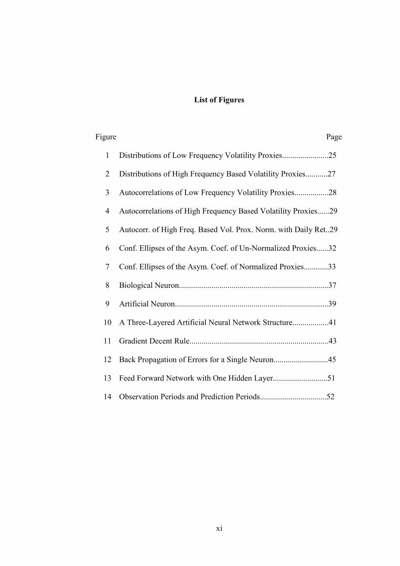
List of Figures

Figure Page

1 Distributions of Low Frequency Volatility Proxies.......................25

2 Distributions of High Frequency Based Volatility Proxies...........27

3 Autocorrelations of Low Frequency Volatility Proxies.................28

4 Autocorrelations of High Frequency Based Volatility Proxies......29

5 Autocorr. of High Freq. Based Vol. Prox. Norm. with Daily Ret..29

6 Conf. Ellipses of the Asym. Coef. of Un-Normalized Proxies......32

7 Conf. Ellipses of the Asym. Coef. of Normalized Proxies............33

8 Biological Neuron..........................................................................37

9 Artificial Neuron............................................................................39

10 A Three-Layered Artificial Neural Network Structure..................41

11 Gradient Decent Rule.....................................................................43

12 Back Propagation of Errors for a Single Neuron...........................45

13 Feed Forward Network with One Hidden Layer...........................51

14 Observation Periods and Prediction Periods.................................52

xii

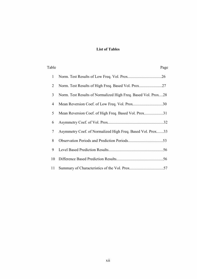
List of Tables

Table Page

1 Norm. Test Results of Low Freq. Vol. Prox..................................26

2 Norm. Test Results of High Freq. Based Vol. Prox.......................27

3 Norm. Test Results of Normalized High Freq. Based Vol. Prox....28

4 Mean Reversion Coef. of Low Freq. Vol. Prox..............................30

5 Mean Reversion Coef. of High Freq. Based Vol. Prox...................31

6 Asymmetry Coef. of Vol. Prox........................................................32

7 Asymmetry Coef. of Normalized High Freq. Based Vol. Prox.......33

8 Observation Periods and Prediction Periods...................................53

9 Level Based Prediction Results.......................................................56

10 Difference Based Prediction Results...............................................56

11 Summary of Characteristics of the Vol. Prox..................................57

1

1. INTRODUCTION

Volatility forecast of the asset prices is a prevailing issue in financial

markets because of its importance for derivative pricing, as well as

investment analysis and market risk management. It is now widely agreed

that obtaining an accurate volatility forecast is a key part of many financial

applications. Since it is considered as a “barometer for the vulnerability of

financial markets and the economy” (Pool & Granger 2003), over the last

two decades academics and professional practitioners in the financial

community devoted a considerable attention how to measure and model

volatility.

However, time series modeling is a challenging procedure due to the

non linear nature of the financial markets. Daily asset returns, for example,

are highly unpredictable, since the complex dynamics governing the market

makes the forecasting procedure somewhat difficult.

Daily return volatility, on the other hand, is more predictable as it

displays some stylized facts such as persistence, mean reversion and

asymmetry. Unfortunately, the data generating process for volatility is

inherently unobservable. That is, unlike from return or volume figures,

volatility is rather a latent variable that should be derived heuristically. Most

of what we make to reveal latent volatility has been either by fitting a

2

parametric econometric models such as GARCH, by studying volatilities

implied by option prices or by analyzing direct indicators such as expost-

squared or absolute return. All of these techniques, valuable as they are,

have also distinct weaknesses.

In recent years ANNs have been proven to be ideal for financial

modeling and hence they have increasingly gained popularity and

advocation as a new alternative modeling technology to more traditional

econometric and statistical approaches. (Dunis & Huang 2001) The

researchers have showed that ANNs have been particularly effective in

capturing the evolution of structural patters disguised in the time-series,

where standard econometric models fail to perform well. (Kuan & White

1994) With their ability to discover hidden patterns in the non-linear and

chaotic systems, ANNs offer the ability to predict market dynamics more

accurately than the current techniques. In the case of foreign exchange rate

markets, where the chaotic and nonlinear dynamics are similarly all over the

place, ANNs are found to be worthwhile according to recent investigations,

some of which are Tenti (1996), Yao et. al. (1996), Gradojevic and Yang

(2000) and Giles et. al. (2001)

In recent studies, high frequency financial data has been broadly used

and been a major focus of volatility forecasting. Especially after the

research of Anderson et. al. (1998a), more and more publications have been

arisen examining the properties of high frequency intraday data, while many

studies had been concentrating on daily squared returns as a measure of

"true volatility" before then. Anderson et. al. (1998a) asserts that, daily

3

squared returns are very noisy measure and cannot reflect the price

fluctuations during the day. High frequency data, on the other hand, carry

more information of the day time transactions. They show that using

sufficiently finely sampled observations provide more accurate and robust

measure of volatility.

4

2. PURPOSE OF THE PAPER

The primary aim of this research is to investigate the predictability of

different volatility indicators for the EUR exchange rate by the means of

Feed Forward Neural Network Model. The paper first defines two kinds of

volatility proxies, namely low frequency proxies and proxies derived from

high frequency data. Low frequency proxies consists of three different

series, which are daily squared returns, daily absolute returns and daily log

range figures. High frequency proxies on the other hand, includes two

indicators. The first one is constructed by summing the squared intraday

returns which is the method for computing realized volatility in the

literature. Second one, which is not appear in the literature according to the

author's knowledge, is constructed by summing the absolute intraday

returns. First, the distributional properties and the characteristics of the

proxies such as persistency, mean reversion and asymmetry are analyzed.

Then, the predictability of these series are investigated. A Feed Forward

Neural Network model, which is an artificial neural network model, is used

to forecast the direction of change in the level of the series for the next day.

Finally, a relationships between the characteristics of the proxies and their

predictability are discussed.

The first conclusion of my result is that, low frequency proxies which

are derived from daily data are more predictive than the proxies derived

5

from high frequency intraday returns. On the other hand, when

normalized with daily returns, high frequency based volatility proxies

become more predictable. The second conclusion is about the stylized facts

of volatility and predictability of volatility series. High frequency based

proxies become normally distributed when they are normalized with daily

returns. These normalized series, unlike from un-normalized ones, do not

display the stylized of volatility. However, their predictability is found to be

superior. This leads us to the inference that the distributional property may

have a stronger effect on predictability than the stylized facts do.

The present paper advances the existing literature in some respects.

First, it redefines the realized volatility using absolute returns and explores

the potential benefits of high frequency data in the one-day-ahead volatility

prediction by the means of artificial neural networks. Second, it searches

whether distributional properties and characteristics of a volatility series

such as persistence, mean reversion and asymmetry have an impact on the

predictability.

The rest of the paper is organized as follows: next section reviews the

related literature, section 4 discusses about the stylized facts of volatility

and analyzes the properties of proposed proxies which will be forecasted,

section 5 briefly introduces the mathematical background and working

principles of the artificial neural networks. Advantages and disadvantages of

neural network models over econometric models are mentioned. Section 6,

Methodology, applies a feed forward neural network model to generate one-

day-ahead forecasts of analyzed volatility proxies. Forecasting results and

6

empirical finding are revealed. Finally, in section 7, the study will be

concluded and further research direction will be proposed.

7

3. LITERATURE REVIEW

Financial markets are very chaotic environments and consist of many

non-linear relationships among various variables. Some researchers claim

that these nonlinearities cause the market exhibit dynamic and unexpected

behaviors. Supporters of this stand employ flexible nonlinear regression

models, such as threshold, smooth transition or Markov switching as a

means of accommodating generic nonlinearity. Such models have been

successfully applied in a wide range of markets, revealing important aspects

of investors’ behavior and market dynamics (Frances & Dick 2000)

The flexibility and adaptability advantages of the artificial neural

network models (ANNs) have attracted the interest of many researchers

from different disciplines including the electrical engineering, robotics and

computer engineering. For the last decade, however, the artificial neural

network models have also attracted the attention of many financial

researchers mostly because of their flexible semi-parametric nature. (Avci

2007) Under mild conditions, an ANN is capable of approximating any

nonlinear function to an arbitrary degree of accuracy, possessing a so-called

universal approximation property. (Hornik et al. 1989 and Hornik 1991)

This is a very important advance for ANNs since the number of possible

nonlinear patters is huge for real-world problems and a good model should

8

be able to approximate them all well. Since ANNs have the ability to

approximate arbitrarily well a large class of functions, they provide

considerable flexibility to uncover hidden non-linear relationships between

a group of individual forecasts and realizations of the variable being

forecasted. (Donaldson & Kamstra 1996)

In the context of financial forecasting, ANNs are considered to be one of

the most promising forecasting techniques. This is why plenty of researchers

have been analyzing the capability of neural networks in financial markets

and why great deal of comparisons are being made between ANNs and

traditional linear econometric methods on the time series forecasting

performance. Under a variety of situations, neural networks have been

found to outperform linear models. Zhang (2001), for example, found that

neural networks are quite effective in linear time-series modeling and

forecasting in a variety of circumstances. According to the author, one

possible explanation is that, neural networks are able to identify the patterns

from noisy data hence give a better forecasts.

Lawrence (1994) asserts that with their ability to discover patterns in

non-linear and chaotic systems, neural networks offer the ability to predict

market directions more accurately than common market analysis techniques

such as technical analysis, fundamental analysis and linear regression. He

tests the Efficient Market Hypothesis using neural networks and refutes its

validity. He concludes his work by expressing that although neural networks

are not perfect in their predictions; they outperform all other linear methods

in terms of forecasting accuracy. Similarly, White (1989b) and Kuan &

9

White (1994) assert that ANNs are particularly effective in capturing

relationship in which linear models fail to perform well.

After giving the importance of artificial neural network models for

financial forecasting in general, the review will hereafter concentrate on two

groups of studies. These are artificial neural network applications for

volatility forecasting and studies which use high frequency financial data for

volatility prediction.

Studies in the first group are focusing on the artificial neural network

models and its comparison with other forecasting techniques. Donaldson

and Kamstra (1996) investigate the use of ANNs to combine different time

series forecasts of stock market volatility from the USA, Canada, Japan and

the UK, in order to obtain more reliable outcomes. They demonstrate that

forecasts, which are combined by ANNs, dominate the results from

traditional combining procedures in terms of out-of-sample forecast

performance and mean squared error comparisons.

Schittenkopf, Dorffner and Dockner (1998) predict the volatility of

Australian stock market and find neural networks outperform ARCH

models. Tino, Schittenkopf and Dorffner (2002) develop a trading algorithm

which is based on predictions of daily volatility differences in financial

indexes DAX and FTSE 100. The main predictive model studied in their

paper is recurrent neural networks. They compare their predictions with the

GARCH family of econometric models and show that while GARCH

models are not able to generate any significant positive profit, by careful use

10

of recurrent neural networks, the market players can generate a statistically

significant excess profit.

Thomaidis (2004) tries to construct a compact model, in which a neural

network model predicts the conditional mean and a GARCH model predicts

the conditional variance of DAX Stock Index. He attempts to forecast one-

day-ahead DAX returns conditionally on the returns observed in the last five

consecutive trading days. Each day when a new observation becomes

available, he re-estimates the parameters of his model. According to his

research, the combination of both models yields better results when a

special attention is paid to the specification of the mean equation which is

generated by his ANN.

Aragones et. al. (2007) explores the predictive power of various

estimates of future volatility of IBEX-35 Index futures by regressing the

realized volatility over the volatility forecasts from different models, such as

GARCH, TARCH and General Regression Neural Network (GRNN)

models. The authors examine the incremental explanatory power of

different models with respect to the implied volatility and they found that

other volatility models accept GRNN, do not include additional predictive

power, when used with implied volatility.

Dunis and Huang (2002) examine the use of Neural Network Regression

(NNR) and Recurrent Neural Network (RNN) models for forecasting and

trading GBP/USD and USD/JPY currency volatility. They analyze the

GARCH model results as a benchmark for their models. According to the

results, RNN models appear as the best modeling approach which retains

11

positive returns allowing transaction costs. They show that for the period

and currencies considered, the currency option market is inefficient and the

option pricing formulae applied by the market participants are inadequate.

The writers also show that the model investigated in the study offer much

more precise indication about the future volatility than the implied volatility

does.

Bekiros and Georgoetsos (2008) construct a volatility trading strategy

based on a Recurrent Neural Network. They attempt to forecast the direction

of change of NASDAQ composite index. In their network design, they use

past index returns and past conditional volatility as inputs, and they try to

estimate the direction of change of the next index value. Their results

indicate that there is a close relationship between asset return signs and asset

return volatilities.

Besides the studies, that compare the forecast accuracy of neural network

models with other linear and nonlinear statistical models, another group of

studies examine the effects of network parameters on the performance.

Zhang (2001) for example, reported that the number of both input and

hidden nodes can strongly affect the forecasting performance. He also found

that simple network models are generally adequate in forecasting linear

time-series.

Despite many conclusions favoring the superiority of ANNs in time

series forecasting, the success of the neural networks are still questionable

in some studies. Tsibouris and Zeidenberg (1995), for example, find up to

only 60% correct sign predictions for four US stocks using a neural network

12

with nine inputs and five hidden layers. In a simulation study conducted by

Markham and Rakes, the performance of ANNs was compared with that of

linear regression problems with varying sample size and noise levels. It was

found that for linear regression problems with different levels of error

variance and sample size, ANNs and linear regression models performed

differently. At lower levels of variance, regression models were better while

at higher levels of variance, ANNs performed better. Experimenting with

simulated data for ideal regression problems, Denton showed that, under

ideal conditions with all assumptions satisfied, there was little difference in

performance between ANNs and regression models. However, under less

ideal conditions such outliers, multicolinearity and model misspecification,

ANNs performed better.

Another set of studies in the literature proposes high frequency intraday

data to be a volatility measure. Andersen et. al (2001), for instance, is

regarded as the seminal paper on using high frequency data in volatility

forecasting, and it shows that the performance of daily GARCH model is

strongly improved by using their new volatility measure called "realized

volatility".

Chortareas, Nankervis and Jiang (2007) focus on forecasting volatility of

high frequency EUR exchange rates and test the out-of-sample forecast

performance of their models including traditional time series volatility

model and realized volatility models. According to their work, advantage of

using high frequency data is confirmed.

13

Martens and Poon (2001) compares the daily volatility forecasts constructed

from daily and intraday data and finds that the higher the intraday frequency

is used, the better the out-of-sample daily volatility forecasts. Martens and

Zein (2004) demonstrates that using high frequency data can improve both

accuracy of measurement and performance of forecasting. Similarly, Hol

and Koopman (2002) shows the ARFIMA model estimated by high

frequency data gives superior performance.

Although there have been plenty of studies using high frequency

financial data and artificial neural networks as a forecasting device

separately, there have not been much research based on both high frequency

data and ANN for exchange rate volatility forecasting. Just to mention a

few, Gradojevic and Yang (2000) employ ANN to predict high-frequency

Canada/US dollar exchange rate. Their results show that ANN model never

performs worse than linear model and always better than the random walk

model in terms of root-mean squared error and direction of change

comparisons. According to the authors, this is not surprising, since ANN is

able to model any non-linear as well as linear functional dependencies.

Finally, they conclude that appropriately selected ANN models with optimal

architectures are superior to random walk and linear competing models for

high-frequency exchange rate forecasting.

Based on the missing gaps in the literature, the aim of this paper is to

explore the potential benefits of using high frequency financial data by the

means of artificial neural network models and analyze the predictability of

high and low frequency volatility proxies.

14

4. VOLATILITY ESTIMATION

Volatility forecasting problem involves a variable of interest that is

unobservable even latent. While evaluating and comparing different

volatility forecasts is a well studied problem, if the variable of interest is

latent, then the problem becomes more complicated. According to Patton

(2004) this complication can be partly resolved if a conditionally unbiased

estimator of the latent variable is available.

The aim of this section is to exploit different volatility estimators and

analyze their characteristics. First, various volatility proxies with different

frequencies, are formed and analyzed with respect to their statistical

properties and distributional characters. They are also inspected whether

they show the stylized facts of volatility that are documented in the

literature. Finally, by using an artificial neural network model in the coming

sections, these proxies are evaluated in terms of their forecastability. The

purpose is to obtain more accurate volatility forecasts by discovering, if any,

the unique information supplied by proposed proxies.

4.1 STYLIZED FACTS ABOUT VOLATILITY

Starting from the publication of ARCH models, a vast quantity of

research confirmed that market volatility exhibits some special properties.

15

These properties, commonly named as stylized facts of volatility, will be

mentioned before introducing volatility proxies in the coming section.

One of the facts, which the volatility of the asset price has, is the

persistence. Being one of the first documented features of volatility,

persistence implies clustering of large moves and small moves in the price

process (Pagan & Schwert 1990). The implication of such volatility

clustering is that volatility shocks today will influence the expectation of

volatility many periods in the future. Mandelbrot (1963) and Fama (1966)

both reported strong evidence that large changes in the price of an asset are

often followed by other large changes and small changes are often followed

by small changes.

Second feature of volatility series is the mean reversion. Mean reversion

of volatility is generally interpreted as meaning that there is a normal level

of volatility to which it will eventually return. There could be periods of

high volatility which will give away at the end, similarly periods of low

volatility will often followed by a rise. In other words, no matter how they

deviate from the normal level for a short period of time, volatility series will

ultimately be pulled back to long-run level over time (Bali and Demistas

2008) Although mean reversion is largely believed as characteristic of

volatility, long-run level of volatility and whether it is constant over all the

time be differ among the market participants. Mean reversion in volatility in

this sense, implies that current information has no effect on the long run

forecast.

16

The third stylized fact of volatility is the asymmetry, which is also

known as the leverage effect (Black, 1976; Christie, 1982) Former ARCH

like models impose the assumption that the conditional volatility of the asset

is affected symmetrically by positive and negative innovations. On the other

hand, today no one believes that positive and negative shocks have the same

impact on the volatility. Veronesi (1999) for instance, argues that markets

tend to overreact to bad news during good economic states and under-react

to positive signals in recessions. More recent research similarly find out that

financial asset returns have significant impact on volatility depending on

their sign. (Poon & Granger 2003)

To sum up, there are several salient features about financial market

volatility which are documented in the literature. They include persistence,

namely volatility clustering, mean reversion and asymmetric impact of

negative and positive innovations. Next section starts defining volatility

proxies, which will be forecasted in section 6 and exploit their properties

related with the ones aforementioned above.

4.2 VOLATILITY PROXIES

4.2.1 LOW FREQUENCY VOLATILITY PROXIES

Squared Return:

Among the various measures proposed as proxy variable for unobserved

volatility, daily squared return is one of the most commonly used one in

empirical financial time series analysis. Many authors tried to develop

17

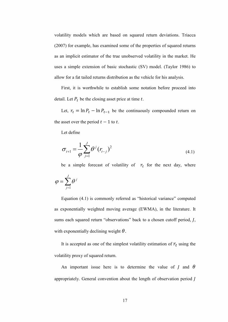
volatility models which are based on squared return deviations. Triacca

(2007) for example, has examined some of the properties of squared returns

as an implicit estimator of the true unobserved volatility in the market. He

uses a simple extension of basic stochastic (SV) model. (Taylor 1986) to

allow for a fat tailed returns distribution as the vehicle for his analysis.

First, it is worthwhile to establish some notation before proceed into

detail. Let �� be the closing asset price at time �.

Let, �� be the continuously compounded return on

the asset over the period � � � to �.

Let define

21

1

1( )

Jj

t t jj

rσ θϕ+ −

=

= ∑

(4.1)

be a simple forecast of volatility of �� for the next day, where

1

Jj

j

ϕ θ=

=∑

Equation (4.1) is commonly referred as “historical variance” computed

as exponentially weighted moving average (EWMA), in the literature. It

sums each squared return “observations” back to a chosen cutoff period, �,

with exponentially declining weight .

It is accepted as one of the simplest volatility estimation of �� using the

volatility proxy of squared return.

An important issue here is to determine the value of � and

appropriately. General convention about the length of observation period �

18

is setting it equal to the length of forecast period. Since we are dealing with

one day ahead volatility forecast, it would be reasonable to chose � as one.

Figlewski (1997), on the other hand, finds that forecast errors are

generally lower if � is chosen much longer than the forecast horizon.

Another complication is about the value of exponentially declining

weight� . Riskmetrics, the most well known user of EWMA for its VAR

modeling, sets as 0,94. Like for the case of �, will be considered as one

in this paper, for the sake of simplicity.

Absolute Return:

Another famous and heavily used volatility proxy is the absolute return.

It has been treated as a measure of risk and its forecastibility has also been

explored by various authors. Modeling the absolute return can be traced

back to Taylor. So called Taylor effect, which could be an appealing fact for

volatility modeling, states that for different stock prices the autocorrelations

of absolute returns are higher than those of squared returns. Many authors

show that absolute return observations may be superior in terms of

forecastibility than squared returns.

For example, Ding, Granger & Engle (1993) claim that absolute value of

returns display stronger persistence and it exhibits consistently higher long

memory behavior than squared return does, making them a better signal for

volatility. Ding and Granger further discover that absolute returns of

different stock markets and foreign exchange rates have corresponding

characteristics.

19

Similarly, Ghysels, Santa-Clara and Valkanov (2005) conclude that

absolute value of returns are less sensitive to large movements in prices,

providing better predictions during periods with jumps.

Giles (2008) undertakes an analysis similar with Triacca (2007), using

absolute returns rather than squared returns. He asserts that absolute returns

may be a better implicit estimator of the true unobserved volatility. He

corrected some errors in Triacca’s results and draw comparisons between

properties of these estimators of volatility.

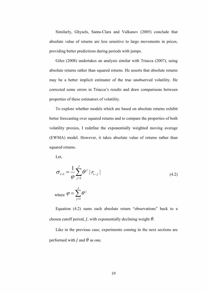
To explore whether models which are based on absolute returns exhibit

better forecasting over squared returns and to compare the properties of both

volatility proxies, I redefine the exponentially weighted moving average

(EWMA) model. However, it takes absolute value of returns rather than

squared returns.

Let,

11

1| |

Jj

t t jj

rσ θϕ+ −

=

= ∑ (4.2)�

where 1

Jj

j

ϕ θ=

=∑

Equation (4.2) sums each absolute return “observations” back to a

chosen cutoff period, �, with exponentially declining weight� .

Like in the previous case, experiments coming in the next sections are

performed with � and as one.

20

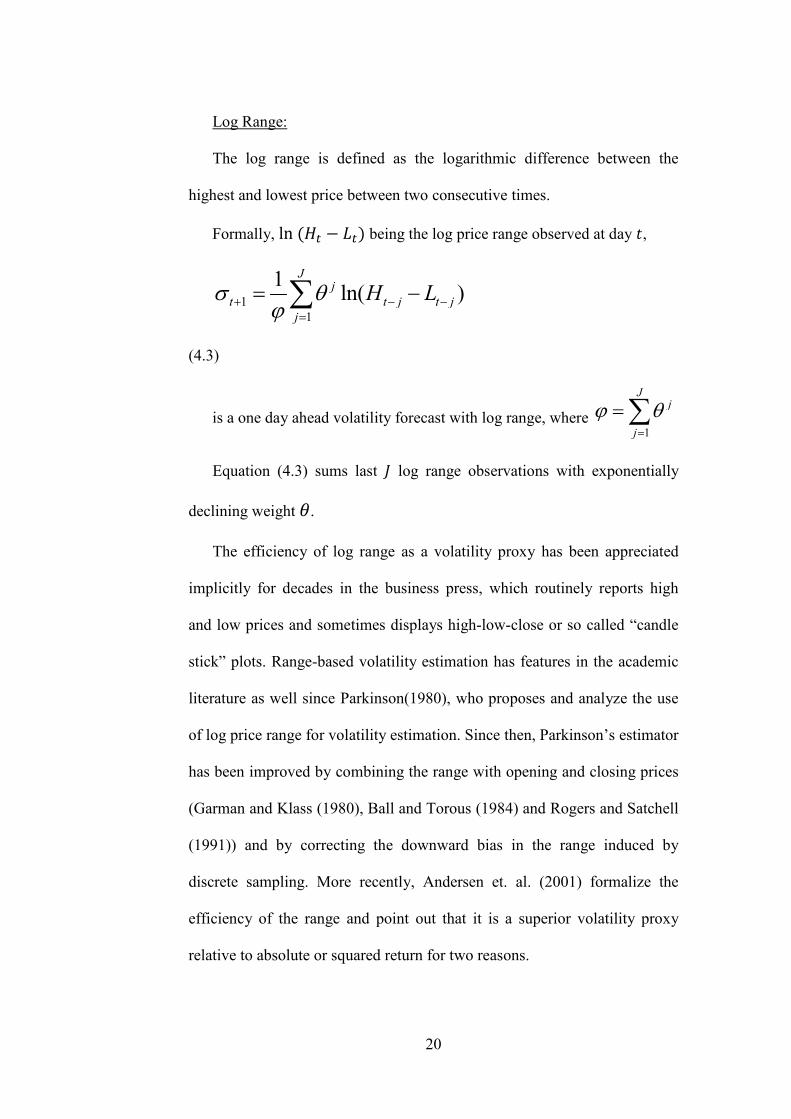
Log Range:

The log range is defined as the logarithmic difference between the

highest and lowest price between two consecutive times.

Formally, �� being the log price range observed at day �,

11

1ln( )

Jj

t t j t jj

H Lσ θϕ+ − −

=

= −∑

(4.3)

is a one day ahead volatility forecast with log range, where 1

Jj

j

ϕ θ=

=∑

Equation (4.3) sums last � log range observations with exponentially

declining weight� .

The efficiency of log range as a volatility proxy has been appreciated

implicitly for decades in the business press, which routinely reports high

and low prices and sometimes displays high-low-close or so called “candle

stick” plots. Range-based volatility estimation has features in the academic

literature as well since Parkinson(1980), who proposes and analyze the use

of log price range for volatility estimation. Since then, Parkinson’s estimator

has been improved by combining the range with opening and closing prices

(Garman and Klass (1980), Ball and Torous (1984) and Rogers and Satchell

(1991)) and by correcting the downward bias in the range induced by

discrete sampling. More recently, Andersen et. al. (2001) formalize the

efficiency of the range and point out that it is a superior volatility proxy

relative to absolute or squared return for two reasons.

21

First, it is more efficient, in the sense that the variance of the

measurement errors associated with the log range is far less than the

measurement errors associated with absolute or squared returns.

Second, the distribution of the log range is very close to Normal, which

makes it attractive as a volatility proxy for Gaussian quasi-maximum

likelihood estimation of stochastic volatility models.

The intuition behind the superior efficiency of the log range is simply

that, on a volatile trading day, with substantial price reversals, return based

measures underestimates the daily volatility because the market happens to

close near the opening price, despite the large intraday price fluctuations.

The log range, in contrast, will take account of the large intraday

movements and correctly indicate a higher estimate of volatility.

4.2.2 HIGH FREQUENCY BASED VOLATILITY PROXIES

Realized Volatility

It has long been known that daily squared returns, absolute returns or

residuals from a regression model for returns are quite noisy proxies for the

conditional variance. These indicators are most of the time contaminated by

noise, which is generally very large relative to that of the signal itself.

(Andersen et. al. 2001)

Andersen et al. (2001) introduce a new idea of using high frequency

intraday data to construct estimates of expost realized volatility. They show

that using sufficiently finely sampled observations provides more accurate

and robust measure of volatility.

22

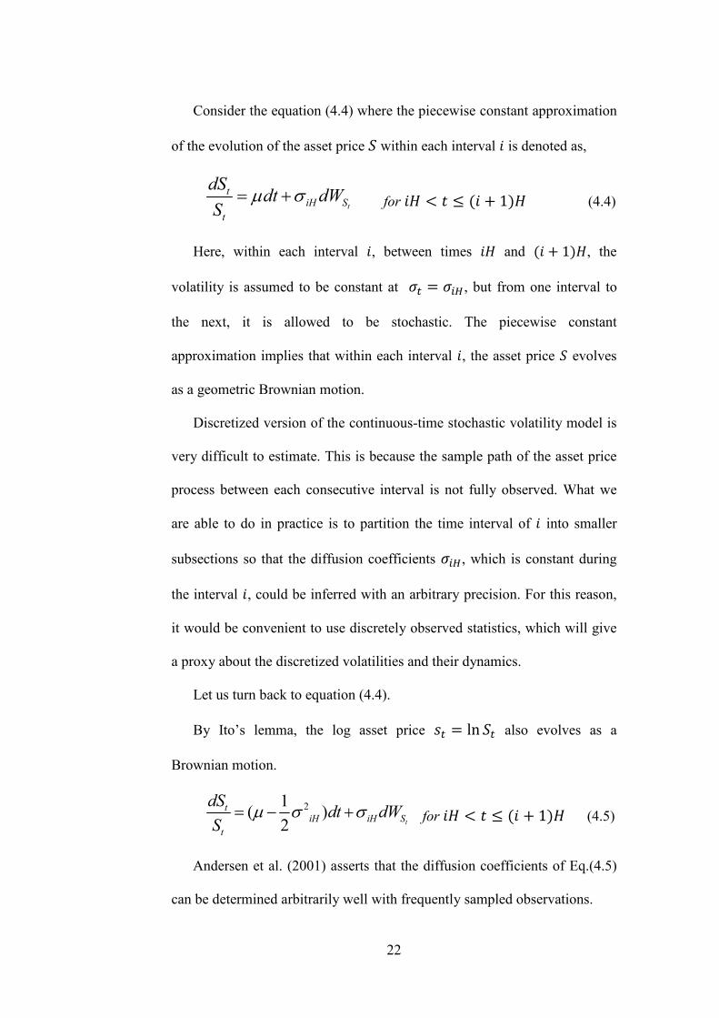
Consider the equation (4.4) where the piecewise constant approximation

of the evolution of the asset price � within each interval � is denoted as,

t

tiH S

t

dSdt dW

Sµ σ= + for �� (4.4)

Here, within each interval �, between times �� and �� , the

volatility is assumed to be constant at �� , but from one interval to

the next, it is allowed to be stochastic. The piecewise constant

approximation implies that within each interval �, the asset price � evolves

as a geometric Brownian motion.

Discretized version of the continuous-time stochastic volatility model is

very difficult to estimate. This is because the sample path of the asset price

process between each consecutive interval is not fully observed. What we

are able to do in practice is to partition the time interval of � into smaller

subsections so that the diffusion coefficients ��, which is constant during

the interval �, could be inferred with an arbitrary precision. For this reason,

it would be convenient to use discretely observed statistics, which will give

a proxy about the discretized volatilities and their dynamics.

Let us turn back to equation (4.4).

By Ito’s lemma, the log asset price �� also evolves as a

Brownian motion.

21( )

2 t

tiH iH S

t

dSdt dW

Sµ σ σ= − + for �� (4.5)

Andersen et al. (2001) asserts that the diffusion coefficients of Eq.(4.5)

can be determined arbitrarily well with frequently sampled observations.

23

To be more clear,

Let 2tσ% be the latent volatility which has been defined over the period

�� . For the diffusion process in Eq.(4.5), the latent volatility

associated with period �� is the integral of the instantaneous

variances aggregated over this period.

( 1)2 2 ( )t i H

i t iHdσ σ τ τ

= +

== ∫% (4.6)

where ( )2σ τ is the instantaneous variance.

Equation (4.6) is called the integrated volatility and it is an expost

measure of latent volatility associated with interval �. Unfortunately, the

integrated volatility is unobservable and therefore needs to be estimated.

Merton (1980) showed that integrated volatility can be approximated

to an arbitrary precision using the sum of the squared returns within the

interval �.

12 2

/0

ˆi t jHj

rδ

δσ−

+=

=∑ for �� (4.7)

where / / ( 1) /ln( ) ln( )t jH t jH t j Hr P Pδ δ δ+ + + −= −

defines continuously

compounded returns sampled � times per period and � shows the length of

�. Note that subscript � indexes the period while indexes the time within

period �.

Andersen et al. (2001) refer to 2ˆiσ as “realized volatility” for period �.

24

In a similar manner, the integrated volatility can also be approximated

using the sum of absolute returns within the interval �.

12

/0

ˆ | |i t jHj

rδ

δσ−

+=

=∑ for �� (4.8)

Although the literature does not contain any reference about the

realized volatility, which is computed as in equation (4.8), this thesis will

compare equation (4.7) and (4.8).

According to the quadratic variation of the diffusion process, which is

not the scope of this text, Equation (4.7) will provide a consistent estimate

of latent volatility over the period �, since

12 2

/0

ˆlim t jH ij

p rδ

δδσ

−

+→∞=

=∑ for �� (4.9)

Hence, as the sampling frequency from a diffusion is increased, the

sum of squared returns converges to the integrated volatility over the fixed

time interval. One of the main reason for the adoption of the realized

volatility concept is that it is free of measurement error as long as δ →∞

However, discrete price quotes and other institutional and behavioral

features of the trading process such as bid-ask bounce make sampling at

very high frequencies impossible or impractical. While the sampling

frequency � goes to very high numbers, it becomes progressively less and

less tolerable as the market microstructure effect emerge. Hence, a tension

arises: the optimal sampling frequency will likely not be the highest

available, but rather intermediate value, ideally high enough to produce a

25

volatility estimate with negligible sampling variation, yet low enough to

avoid microstructure bias. The choice of the underlying return frequency is

therefore critical. General tendency about the sampling frequency for the

method of realized volatility is that the sampling intervals should not be

shorter than five minutes. Considering the findings of the literature, the

sampling interval, �, is chosen to be 10 minutes in the experiments, which

are conducted in the next section.

4.3 ANALYSIS OF VOLATILITY PROXIES

The analysis presented in this section based on EUR/USD exchange rate

data which is publicly available at http://freeserv.dukascopy.com/exp/. The

sample period starts at July 21, 2003 and ends at February 8, 2010. Low

frequency proxies are computed with daily data which consists of daily

opening and closing prices as well as lowest and highest bids. High

frequency based proxies however, are based on data sample by 10 minutes

interval.

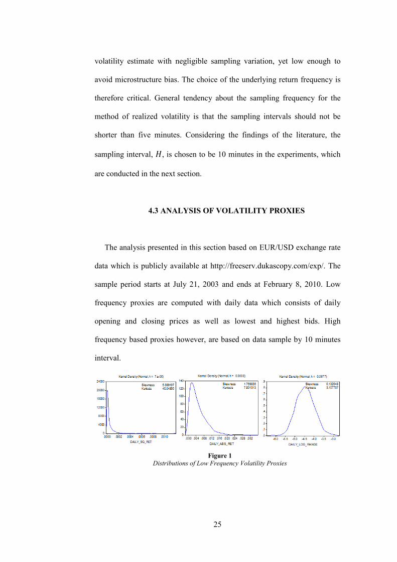
Figure 1 Distributions of Low Frequency Volatility Proxies

26

4.3.1 DISTRUBUTIONS

The distributions of low frequency volatility proxies are graphed in

Figure 1. The skewness and kurtosis coefficients are displayed in the top

right corner of each plot. The distributions of daily square returns and daily

absolute returns are obviously non-normal and leaptokurtic. Daily log range,

on the other hand, seems to be normal distributed with a skewness

coefficient of 0,132 and a kurthosis coefficient of 3,158.

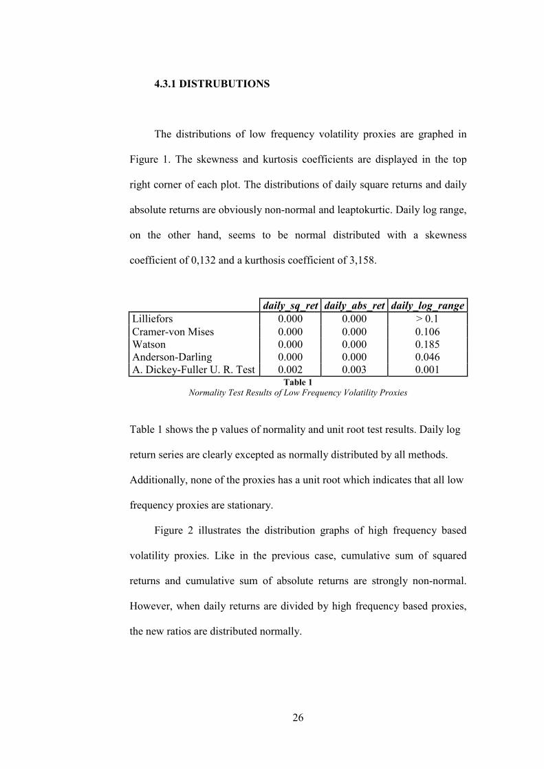
Table 1 Normality Test Results of Low Frequency Volatility Proxies

Table 1 shows the p values of normality and unit root test results. Daily log

return series are clearly excepted as normally distributed by all methods.

Additionally, none of the proxies has a unit root which indicates that all low

frequency proxies are stationary.

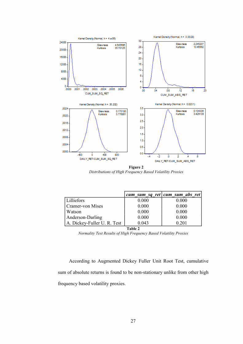
Figure 2 illustrates the distribution graphs of high frequency based

volatility proxies. Like in the previous case, cumulative sum of squared

returns and cumulative sum of absolute returns are strongly non-normal.

However, when daily returns are divided by high frequency based proxies,

the new ratios are distributed normally.

daily_sq_ret daily_abs_ret daily_log_range Lilliefors 0.000 0.000 > 0.1 Cramer-von Mises 0.000 0.000 0.106 Watson 0.000 0.000 0.185 Anderson-Darling 0.000 0.000 0.046 A. Dickey-Fuller U. R. Test 0.002 0.003 0.001

27

cum_sum_sq_ret cum_sum_abs_ret Lilliefors 0.000 0.000 Cramer-von Mises 0.000 0.000 Watson 0.000 0.000 Anderson-Darling 0.000 0.000 A. Dickey-Fuller U. R. Test 0.043 0.201

Table 2 Normality Test Results of High Frequency Based Volatility Proxies

According to Augmented Dickey Fuller Unit Root Test, cumulative

sum of absolute returns is found to be non-stationary unlike from other high

frequency based volatility proxies.

Figure 2 Distributions of High Frequency Based Volatility Proxies

28

daily_ret /cum_sum_sq_ret

daily_ret /cum_sum_abs_ret

Lilliefors 0.068 > 0.1 Cramer-von Mises 0.054 0.565 Watson 0.058 0.534 Anderson-Darling 0.064 0.469 A. Dickey-Fuller U. R. Test 0.000 0.000

Table 3 Normality Test Results of Normalized High Frequency Based Volatility Proxies

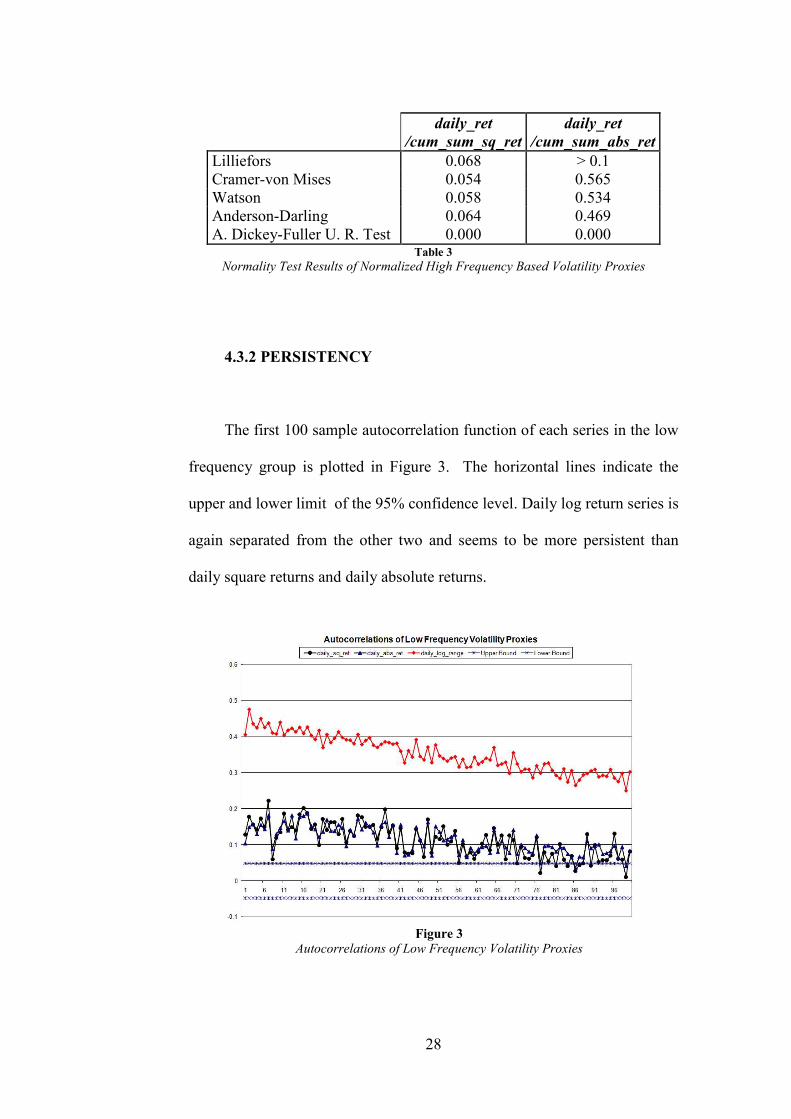
4.3.2 PERSISTENCY

The first 100 sample autocorrelation function of each series in the low

frequency group is plotted in Figure 3. The horizontal lines indicate the

upper and lower limit of the 95% confidence level. Daily log return series is

again separated from the other two and seems to be more persistent than

daily square returns and daily absolute returns.

Figure 3 Autocorrelations of Low Frequency Volatility Proxies

29

Autocorrelations of cumulative sum of squared returns and cumulative

sum of absolute returns are graphed on Figure 4. It is obviously seen from

the figure that the autocorrelations of high frequency volatility proxies are

much more stronger than those of low frequency proxies, indicating a

stronger persistence of longer memory.

Figure 4 Autocorrelations of High Frequency Based Volatility Proxies

Figure 5 Autocorrelations of High Frequency Based Volatility Proxies Normalized

with Daily Returns

30

Persistency of normalized high frequency based proxies are also

graphed. Figure 5 demonstrates that with 95% confidence level, the new

series have nearly no memory.

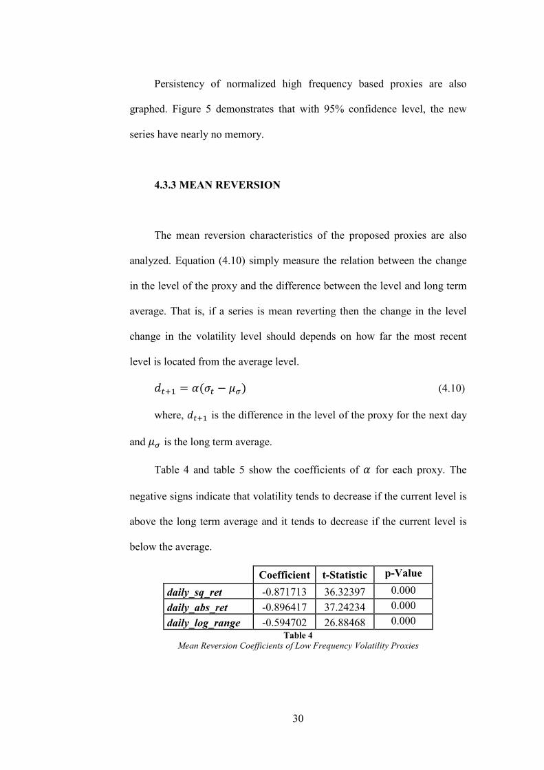
4.3.3 MEAN REVERSION

The mean reversion characteristics of the proposed proxies are also

analyzed. Equation (4.10) simply measure the relation between the change

in the level of the proxy and the difference between the level and long term

average. That is, if a series is mean reverting then the change in the level

change in the volatility level should depends on how far the most recent

level is located from the average level.

!�" � #�� $%� (4.10)

where, !�" is the difference in the level of the proxy for the next day

and $% is the long term average.

Table 4 and table 5 show the coefficients of # for each proxy. The

negative signs indicate that volatility tends to decrease if the current level is

above the long term average and it tends to decrease if the current level is

below the average.

Coefficient t-Statistic p-Value

daily_sq_ret -0.871713 36.32397 0.000

daily_abs_ret -0.896417 37.24234 0.000

daily_log_range -0.594702 26.88468 0.000 Table 4

Mean Reversion Coefficients of Low Frequency Volatility Proxies

31

Coefficient t-Statistic p-Value

cum_sum_sq_ret -0.261744 16.03683 0.000

cum_sum_abs_ret -0.135264 11.13005 0.000

daily_ret/cum_sum_sq_ret -1.048143 43.37366 0.000

daiy_ret/cum_sum_abs_ret -1.033417 42.74157 0.000 Table 5

Mean Reversion Coefficients of High Frequency Based Volatility Proxies

According to the tables above, the mean reversion is a common feature

among the proxies.

4.3.4 ASYMMETRY

In order to test the asymmetric property of each proxy, Equation (4.11)

is formed.

Let !� be volatility change between day t-1 and t,

!� � #!� � &!�

" (4.11)

where,

!� � !��'�!� � (

!� � (��)*

and

!�" � !��'�!� + (

!�" � (��)*

Equation (4.11) detects whether the direction of previous day's

volatility change has an impact on the current level of volatility. To be more

clear, if the coefficients of # and & are statistically significant and they are

different, then the volatility proxy exhibits asymmetric property.

32

The results are shown on Table 6. The most important result about the

asymmetry test is that the negative changes are more decisive on the next

volatility level. This is because all ALPHAs are greater than BETAs.

Variable Coefficient t-Statistic p-Value

daily_sq_ret ALPHA 2.195606 28.64257 0.000 BETA 0.172306 8.49306 0.000

daily_abs_ret ALPHA 1.83092 51.35204 0.000 BETA 0.360315 23.04504 0.000

daily_log_range ALPHA 1.095819 218.7453 0.000

BETA 0.905743 196.4014 0.000

cum_sum_sq_ret ALPHA 1.433999 97.47248 0.000

BETA 0.603751 61.47563 0.000

cum_sum_abs_ret ALPHA 1.159595 238.3588 0.000

BETA 0.85032 206.0587 0.000

Table 6 Asymmetry Coefficients of Volatility Proxies

Figure 6 Confidence Ellipses of the Asymmetry Coefficients of Un-normalized Proxies

33

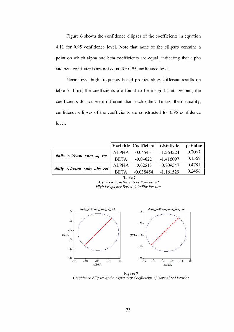
Figure 6 shows the confidence ellipses of the coefficients in equation

4.11 for 0.95 confidence level. Note that none of the ellipses contains a

point on which alpha and beta coefficients are equal, indicating that alpha

and beta coefficients are not equal for 0.95 confidence level.

Normalized high frequency based proxies show different results on

table 7. First, the coefficients are found to be insignificant. Second, the

coefficients do not seem different than each other. To test their equality,

confidence ellipses of the coefficients are constructed for 0.95 confidence

level.

Variable Coefficient t-Statistic p-Value

daily_ret/cum_sum_sq_ret ALPHA -0.045451 -1.263224 0.2067

BETA -0.04622 -1.416097 0.1569

daily_ret/cum_sum_abs_ret ALPHA -0.02513 -0.709547 0.4781

BETA -0.038454 -1.161529 0.2456

Asymmetry Coefficients of Normalized High Frequency Based Volatility Proxies

Table 7

Figure 7 Confidence Ellipses of the Asymmetry Coefficients of Normalized Proxies

34

On figure 7, the red lines display the points on which the coefficients

are equal. Since the ellipses includes red lines, the coefficients are not

statistically different, indicating that the high frequency based proxies

normalized with daily returns do not have the property of asymmetry.

The analysis in this section are performed in order to test whether the

proposed volatility proxies show the stylized facts of volatility, such as

persistence, mean reversion and asymmetry. Distributional properties are

also examined.

To sum the findings, high frequency based volatility proxies

normalized with daily returns, do not show the stylized facts of volatility

accept mean reversion, which is common among all the proxies. However,

these proxies are distributed normally. Cumulative sum of squared returns

and cumulative sum of absolute returns on the other hand, display all the

characteristics of volatility but they are non-normal.

In section 6, the forecastability of these proxies are compared and

whether the distributional characters and stylized facts influence the

forecastability is discussed.

35

5. ARTIFICIAL NEURAL NETWORKS

5.1 INTRODUCTION

Recent years have seen a dramatic improvement in the communication

technologies and computer based analysis techniques. Complex

mathematical algorithms and financial models, which were nearly

impossible to analyze before, are no longer problematic due to the currently

reached advance computational speed. Contrary to the past, chaotic patterns

and non-linear behaviors of financial markets are more accountable today.

As empirical studies suggest computer based intelligent models are very

good at capturing these non-linear behaviors. One of the most promising

and interesting computer technology, which carries a significant potential

for financial forecasting is Artificial Intelligence (AI).

AI has been described as the study and design of systems that perceives

its environment and takes actions which maximizes its chance of success.

The field was founded on the claim that intelligence, which is the central

property of human beings, can be precisely described that it can be

simulated by software. In some limited ways, AI can behave like a human

being. It embodies the ability to adapt to the environment and ascertain from

its past experience.

36

An Artificial Neural Network (ANN) is one of the AI tools, which is

revealed from the biological science. The researchers display that ANNs are

more powerful in financial forecasting than the classical econometric

models because of their important advantages. (Gestel & Tony 2005) This

section briefly introduces the concept of Artificial Neural Networks

including the source of inspiration, theoretical foundations and relation with

financial applications. First, the biological background is given. Then the

mathematical of the network is constructed. Finally, according to the

literature, the advantages and disadvantages of ANN as a forecasting

method is criticized.

5.2 BIOLOGICAL BACKGROUND

Artificial Neural Network models were derived from the biological

sciences, which study how neuroanatomy of the living animal works. The

inspiration comes from the architecture of the nervous system which enables

living animals to perform complex tasks instinctively. ANNs try to imitate

the working mechanism of their biological counterparts and implement the

principles of biological learning process mathematically. They are designed

to capture the ability to be able to recognize some behaviors and situations

in a way that human brain process data and derive information from

experience.

As in the structure of brain, an ANN is compo

processing elements, called neurons, which are operating in parallel. The

function of these neurons is mainly determined by network structure and

connection strengths. While the network faces with different situations, the

connections be

learning is performed.

To develop a feel for an analogy, let us consider f

neurobiology. Figure 8

central processing unit of a nervous system. Information or signals are

transmitted unidirectional over the channels called axons. An axon provides

an output path and carries the response of a neuron to th

Information is received by the next neuron through its dendrites. The

connection between an axon and a dendrite, through which the neurons

communicate each other, is called synapse. It is through these synapses that

the most learning is carried

the incoming signals. Exciting or inhibiting the associated neuron activity

37

As in the structure of brain, an ANN is composed of many simple




connections between neurons adjust their synaptic strengths so that the

learning is performed.

To develop a feel for an analogy, let us consider f

neurobiology. Figure 8 provides a typical biological neuron which is the



an output path and carries the response of a neuron to th




the most learning is carried out by releasing neurotransmitters according to


Figure 8 Biological Neuron

sed of many simple




tween neurons adjust their synaptic strengths so that the

To develop a feel for an analogy, let us consider facts from

provides a typical biological neuron which is the



an output path and carries the response of a neuron to the next one.




out by releasing neurotransmitters according to


38

depends on the volume of the signal as well as the intensity and the content

of the neurotransmitter. Learning is usually done by either adjusting

excretion mechanism of the existing synapses or creating new synapses. In

the human brain nearly 100 billion neurons are organized in clusters over

1014 synapses.

The learning process of the neural networks can be linked to the way a

child learns how to walk. For example, the child has to be exposed to a

number of walking trials, many of which result unsuccessful. However,

during every trial, additional information is stored in the synaptic

connections. Child’s neurons, which are responsible for maintaining the

balance of the body, add up all the beneficial signals and inhibit all the

unnecessary and spoiling ones. Eventually, the synaptic weights are adjusted

and fixed by trial and error, so that the balance of the body is maintained

during walking.

5.3 MATHEMATICAL MODEL

5.3.1 ARTIFICIAL NEURON MODEL

Working principle of an artificial neuron is similar to one, employed in

the human brain. Figure 9 provides an artificial neuron, which gets � number

of inputs, every of which is connected to the neuron with a weight

associated with the input. Positive weights activate the neuron while

negative weights inhibit it. The neuron sums all the signals it receives, with

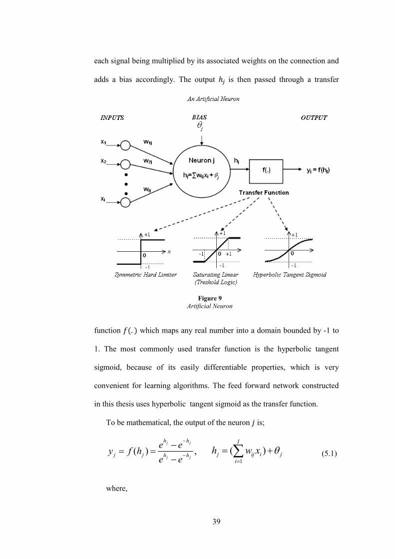
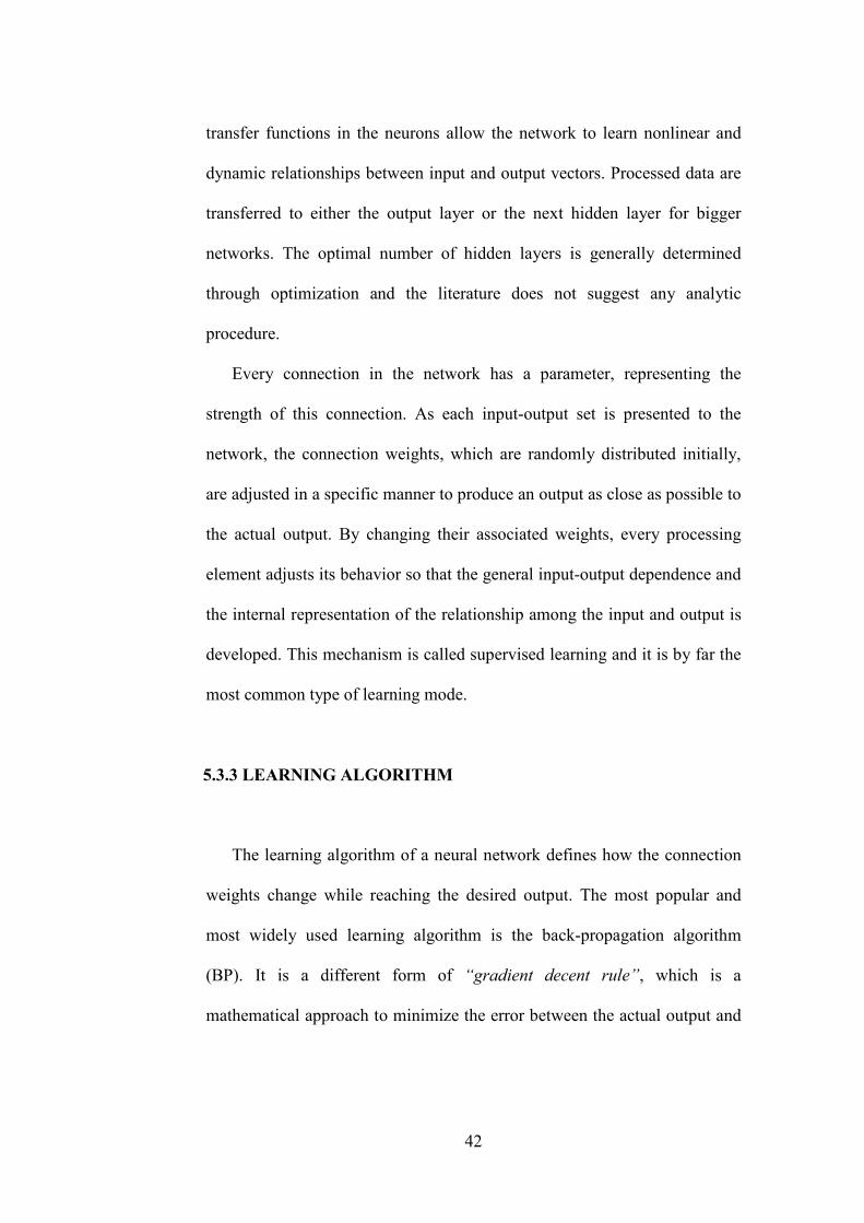
39

each signal being multiplied by its associated weights on the connection and

adds a bias accordingly. The output ,- is then passed through a transfer

function '�. � which maps any real number into a domain bounded by -1 to

1. The most commonly used transfer function is the hyperbolic tangent

sigmoid, because of its easily differentiable properties, which is very

convenient for learning algorithms. The feed forward network constructed

in this thesis uses hyperbolic tangent sigmoid as the transfer function.

To be mathematical, the output of the neuron is;

( ) ,j j

j j

h h

j j h h

e ey f h

e e

−

−

−= =

− 1

( )I

j ij i ji

h w x θ=

= +∑ (5.1)

where,

Figure 9 Artificial Neuron

40

- is the bias of neuron

*�- is the connection strength associated with input /�-

0 is the number of input connection to the neuron

'�. � is the bounded nonlinear transfer function

Kalman and Kwasny (1992) argue that the hyperbolic tangent function is

the ideal transfer function. According to Master (1993) on the other hand,

the shape of the function has little effect on a network although it can have a

significant impact on the training speed. Other common transfer functions

include;

Symmetric Hard Limiter:

( ) 1j jy f h= = − if 0jh < , 0 otherwise

Saturating Linear:

( )j j jy f h h= = if 1 1jh− < <

1 if 1jh ≥

1− if 1jh ≤ −

5.3.2 FEED FORWARD NETWORK STRUCTURE

Although ANNs were inspired by the biological sciences, they are still

far from resembling the architecture of the simplest biological network.

Despite the enormous complexity of the biological networks, a typical

neural network is composed of much fewer neurons arranged in groups or

layers.

41

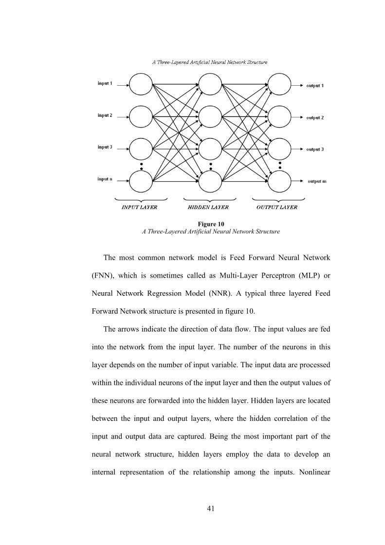
Figure 10

A Three-Layered Artificial Neural Network Structure

The most common network model is Feed Forward Neural Network

(FNN), which is sometimes called as Multi-Layer Perceptron (MLP) or

Neural Network Regression Model (NNR). A typical three layered Feed

Forward Network structure is presented in figure 10.

The arrows indicate the direction of data flow. The input values are fed

into the network from the input layer. The number of the neurons in this

layer depends on the number of input variable. The input data are processed

within the individual neurons of the input layer and then the output values of

these neurons are forwarded into the hidden layer. Hidden layers are located

between the input and output layers, where the hidden correlation of the

input and output data are captured. Being the most important part of the

neural network structure, hidden layers employ the data to develop an

internal representation of the relationship among the inputs. Nonlinear

42

transfer functions in the neurons allow the network to learn nonlinear and

dynamic relationships between input and output vectors. Processed data are

transferred to either the output layer or the next hidden layer for bigger

networks. The optimal number of hidden layers is generally determined

through optimization and the literature does not suggest any analytic

procedure.

Every connection in the network has a parameter, representing the

strength of this connection. As each input-output set is presented to the

network, the connection weights, which are randomly distributed initially,

are adjusted in a specific manner to produce an output as close as possible to

the actual output. By changing their associated weights, every processing

element adjusts its behavior so that the general input-output dependence and

the internal representation of the relationship among the input and output is

developed. This mechanism is called supervised learning and it is by far the

most common type of learning mode.

5.3.3 LEARNING ALGORITHM

The learning algorithm of a neural network defines how the connection

weights change while reaching the desired output. The most popular and

most widely used learning algorithm is the back-propagation algorithm

(BP). It is a different form of “gradient decent rule”, which is a

mathematical approach to minimize the error between the actual output and

43

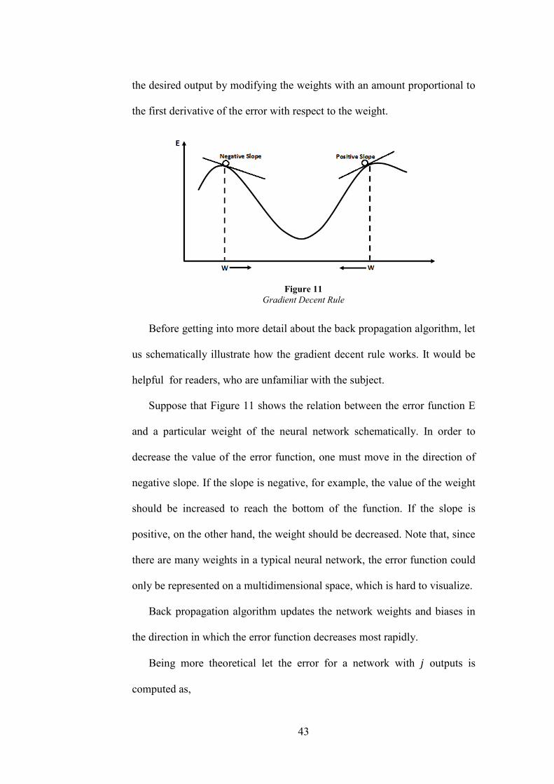
the desired output by modifying the weights with an amount proportional to

the first derivative of the error with respect to the weight.

Before getting into more detail about the back propagation algorithm, let

us schematically illustrate how the gradient decent rule works. It would be

helpful for readers, who are unfamiliar with the subject.

Suppose that Figure 11 shows the relation between the error function E

and a particular weight of the neural network schematically. In order to

decrease the value of the error function, one must move in the direction of

negative slope. If the slope is negative, for example, the value of the weight

should be increased to reach the bottom of the function. If the slope is

positive, on the other hand, the weight should be decreased. Note that, since

there are many weights in a typical neural network, the error function could

only be represented on a multidimensional space, which is hard to visualize.

Back propagation algorithm updates the network weights and biases in

the direction in which the error function decreases most rapidly.

Being more theoretical let the error for a network with outputs is

computed as,

Figure 11 Gradient Decent Rule

44

21( )

2 j jj

E t y= −∑ (5.2)

where

1 is the total error of the entire network, �- is the target output for the �2

neuron, 3- is the actual output of the �2 neuron.

Since we are dealing with only the �2 neuron for clarity, we can omit

the summation. Hence, the equation 5.2 could be rewritten as

21

( )2j j je t y= − (5.3)

where

4- is the total error associated with the �2 neuron.

Additionally, from equation 5.1,

( )j jy f h=, 1

( )I

j ij i ji

h w x θ=

= +∑

where

(.)f is a non-linear transfer function.

Back-propagation algorithm moves through “weight space” of the

neuron in proportion to the gradient of the error function with respect to

each weight. In order to do that the partial derivative of the error with

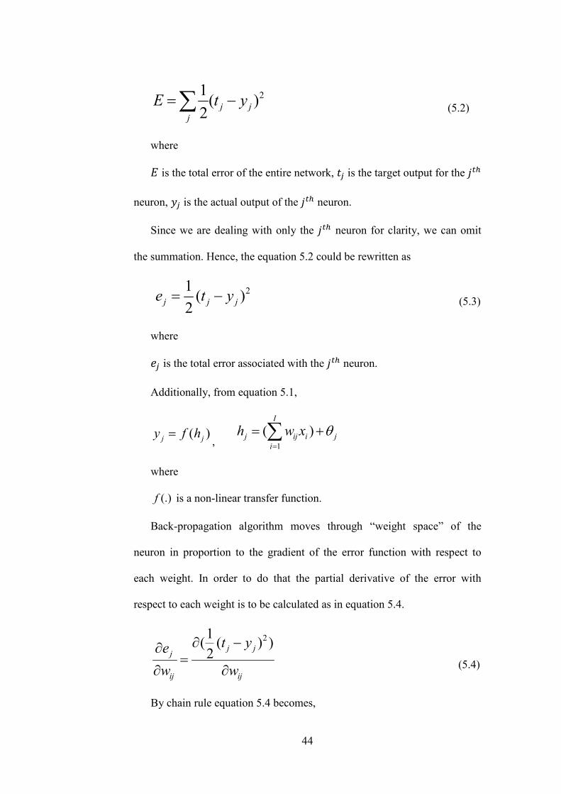
respect to each weight is to be calculated as in equation 5.4.

21( ( ) )2 j j

j

ij ij

t ye

w w

∂ −∂=

∂ ∂ (5.4)

By chain rule equation 5.4 becomes,

45

21( ( ) )2 . .

j jj j

j j ij

t y y h

y h w

∂ − ∂ ∂

∂ ∂ ∂ (5.5)

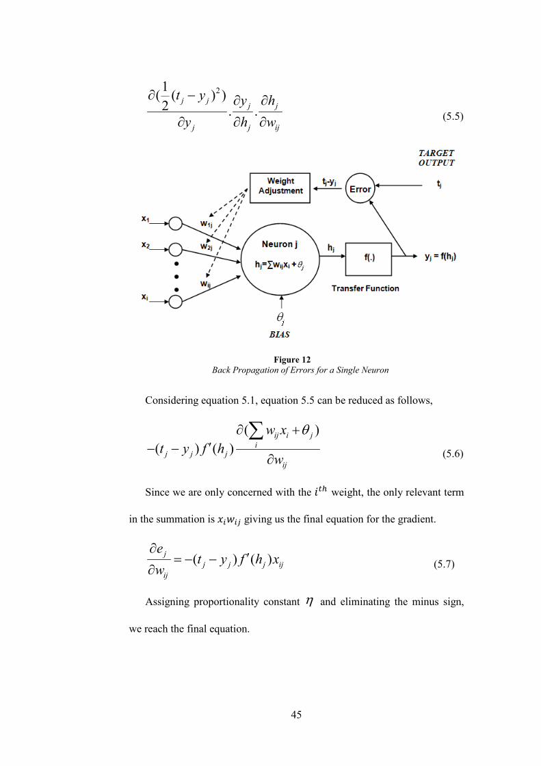
Considering equation 5.1, equation 5.5 can be reduced as follows,

( )( ) ( )

ij i ji

j j jij

w xt y f h

w

θ∂ +′− −

∂

∑ (5.6)

Since we are only concerned with the ��2 weight, the only relevant term

in the summation is /�*�- giving us the final equation for the gradient.

( ) ( )jj j j ij

ij

et y f h x

w

∂′= − −

∂ (5.7)

Assigning proportionality constant η and eliminating the minus sign,

we reach the final equation.

Figure 12 Back Propagation of Errors for a Single Neuron

46

( ) ( )ij j j j ijw t y f h xη ′∆ = − (5.8)

where

η is the learning rate ( 0 1η< < ) The learning rate η determines

how fast the weights are modified. If it is too high, the gradient decent

algorithm may overshoot the solution, on the other hand if it is set too low

then it will yield longer training time.

Equation 5.8 computes the change for every weight in each iteration.

Note that, as mentioned before, it is very important for the transfer function

'�. � to be differentiable. Back-propagation learning algorithm needs the

derivative of the transfer function to compute the weight change.

The weight adjustments which are computed in equation 5.8 are then

added to the previous values. That is,

New weight value = ij ij ijw w w′= + ∆

where,

ijw′ is the previous weight term.

The error surface of a typical problem is not smooth but containing

many hills, ravines and chasms as a result, equation 5.8 is susceptible

becoming trapped in local minima. A momentum term is generally added to

equation 8 to avoid the model’s search direction from swinging back and

forth widely (Tan, 2000).

The weight adjustment term of equation 5.8 will then becomes,

(1 ) ( ) ( )ij j ij ij ijw M f h x M w wη ′ ′ ′′∆ = − + − (5.9)

where,

47

M is the momentum term, ijw′′ is the weight before the previous weight

ijw′ . Momentum term does not allow weight change to make adjustment

cycles.

5.4 STRENGHTS AND WEAKNESSES of ANNs

In the field of finance, where the environment is chaotic and non-linear

dynamic relationships are all over the place, ANNs could be more useful

than conventional computational techniques and statistical models for

prediction purposes.

First, in contrast to time series models for which the identification of the

model to fit a particular time series of data is very difficult, ANNs do not

depend on assumptions regarding the data but adopt their selves to the data.

(Davies 1995) The researchers does not need to know the necessary rules to

construct a prediction model, instead, he/she trained the network with

previous samples of data and the network adopt to changing market

behavior.

Second, ANNs are well suited to solve non-linear problems. This makes

them particularly useful in dynamic and volatile environments. They are

capable of approximating complex functional dependencies among market

variables arbitrarily well. (White 1989a) ANNs’ strength lies in the fact that

they can comprehend subtle patterns and detect correlations in hundreds of

variables without being stifled by detail. It is this feature in analyzing

relationships between a large numbers of market variables. (Hamid 2004)

48

Finally, one of the most important advantages of ANNs over other

techniques is the fault tolerance. The fault tolerance characteristic is a result

of distributed information throughout the synaptic connections in the

network. This wide distribution of information also allows the neural

pathways to deal well with noisy data. (Cifter & Ozun 2007) Even when a

data set is noisy or has irrelevant inputs, the network can learn important

features of the data. According to Tan (2000), ANNs are very tolerant of

noisy and incomplete data sets because of the fact that information is

duplicated many times in the complex network connections.

Despite their various advantages, ANNs have also some weaknesses

over conventional methods. One of the major shortcomings is their lack of

explanation for the models they create. The process through which an ANN

produces an output cannot be debugged or decomposed. The way they

capture the nonlinearities is very hard to understand in detail.

Second handicap for the neural networks is that the pre-processing of the

data, including the data selection and presentation to the network and post-

processing of the outputs require significant amount of work (Gradojevic

and Yang, 2000). As Ripley (1993) states “the design and learning for

neural network” is very hard.

Final shortcoming which worth noting is that a neural network may

“overfit” the data (Hamid, 2004). Kean (1993) defines the overfitting

problem for a network as lack of learning significant relationships between

input and output, but rather memorizing trivial relationships. According to

49

the literature, there are some solutions preventing overfitting such as using

fuzzy logic, genetic algorithm windowing,

According to Hornik et. al. (1989) neural networks are similar to linear

and nonlinear least squares regression models and can be viewed as an

alternative statistical approach to solving the least squares problem.

However unlike any other classical statistical methodology, with their

weight and bias components adjusted according to the experience, neural

networks can learn from the historical data. This gives the network intuitive

predictability and intelligence (Gradojevic & Yang 2000).

50

6. METHODOLOGY

This section discusses the methodology used to develop a neural network

based volatility prediction model. Feed Forward Neural Network is chosen

as a forecasting device in order to forecast the direction of the volatility

level and volatility change for the next day. Volatility proxies which have

been introduced in section four, will be analyzed in terms of their

forecastability. The section first introduces the parameters of the network,

which is used by constructing the network. Then the experimental method,

the procedure of data introduction and the post-processing of the outputs are

explained. Finally, the experimental results are examined and discussed.

6.1 NETWORK PARAMETERS

6.1.1 TRAINING FUNCTION

Weights and biases are updated according to the BFGS (Broyden-

Fletcher-Goldfarb-Shanno) quasi Newton method. To be simple, since the

theoretical background is beyond the scope of this text, this method

determines the search direction by using back propagation algorithm.

6.1.2 LEARNING FUNCTION

Gradient decent function,

calculate the weight and bias cha

6.1.3 PERFORMANCE FUNCTION

Mean squared error is used as the performance function w

calculated as in Equation 5.2

6.1.4 NUMBER OF LAYERS AND NEURONS

Literature proposes conflicting formulas to calculate the

of hidden layers and number layers in the hidden layers. There is not a

generally accepted rule about the size of the network. The network should

be large enough to capture the nonlinear functions in the data, at the same

time it should be simple in

Feed Forward Neural Network with One Hidden Layer

51

6.1.2 LEARNING FUNCTION

Gradient decent function, which is explained in section five

calculate the weight and bias changes according to the Equation 5.9

6.1.3 PERFORMANCE FUNCTION

Mean squared error is used as the performance function w

calculated as in Equation 5.2

6.1.4 NUMBER OF LAYERS AND NEURONS

Literature proposes conflicting formulas to calculate the




time it should be simple in order to be trained quickly. Three layer feed

Figure 13 Feed Forward Neural Network with One Hidden Layer

which is explained in section five, is used to

nges according to the Equation 5.9

Mean squared error is used as the performance function which is

Literature proposes conflicting formulas to calculate the optimal number




order to be trained quickly. Three layer feed

Feed Forward Neural Network with One Hidden Layer

52

forward neural network with one hidden layer is used in the experiment.

Figure 13 shows a schematic representation. The number of neurons in the

hidden layer is set to 5, 10 and 20 respectively. Logarithmic tangent

sigmoid transfer function is employed in the neurons.

6.2 EXPERIMENTAL METHOD

The sample period is divided into subperiods which are called

observation period and prediction period. During the observation period, the

network is trained and the learning is performed. During the prediction

period which is subsequent to the observation period, the network weights

and biases are kept constant and the prediction power of the model is

computed. As the Figure 14 shows, the time window is shifted until the total

period is depleted.

Figure 14 Observation Periods and Prediction Periods

53

The most important point here is how long the observation period and

prediction period should be. The observation period should be long enough

to enable the network to learn the dynamics in the data sufficiently well. On

the other hand, it should not exceed a certain limit , toward which the oldest

data become useless for the prediction. Similarly, the length of the

prediction period should be reasonable as the model parameters turn out to

be irrelevant from some point on. Considering these facts, the lengths of the

observation period and prediction period are set at 1000 and 100

respectively.

Observation Period Prediction Period 1 21 Jul 2003-21 May 2007 22 May 2007-8 Oct 2007 2 8 Dec 2003-8 Oct 2007 9 Oct 2007-25 Feb 2008 3 26 Apr 2004-25 Feb 2008 26 Feb 2008-14 Jul 2008 4 13 Sep 2004-14 Jul 2008 15 Jul 2008-1 Dec 2008 5 31 Jan 2005-1 Dec 2008 2 Dec 2008-20 Apr 2009 6 20 Jun 2005-20 Apr 2009 21 Apr 2009-7 Sep 2009 7 7 Nov 2005-7 Sep 2009 8 Sep 2009- 25 Jan 2010 8 27 Mar 2006-25 Jan 2010 26 Jan 2010-8 Fab 2010

Table 8 Observation Periods and Prediction Periods

Table 9 displays the starting and ending points of the periods.

6.3 INPUT&TARGET SELECTION

This section explains what the neural network gets as input and what it

assumes as the target. The experiment is conducted with four different input

and target combinations which are stated as follows;

Level Based Prediction:

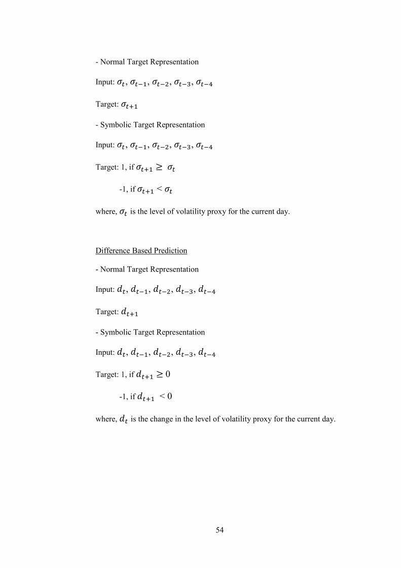
54

- Normal Target Representation

Input: ��, ��, ��5, ��6, ��7

Target: ��"

- Symbolic Target Representation

Input: ��, ��, ��5, ��6, ��7

Target: 1, if ��" 8 ��

-1, if ��" < ��

where, �� is the level of volatility proxy for the current day.

Difference Based Prediction

- Normal Target Representation

Input: !�, !�, !�5, !�6, !�7

Target: !�"

- Symbolic Target Representation

Input: !�, !�, !�5, !�6, !�7

Target: 1, if !�" 8 0

-1, if !�" < 0

where, !� is the change in the level of volatility proxy for the current day.

55

6.4 POST PROCESSING OF THE OUTPUTS

This section explains how the neural network outputs are treated and the

success rate is evaluated.

Normal Target Representation

if, �)9�:9��" � �;�<4�� = ��;�<4��" � �;�<4�� + (

then, �9>>4��

otherwise, ';�?9�4

Symbolic Target Representation

if, )9�:9��" = �;�<4��" + (

then, �9>>4��

otherwise, ';�?9�4

6.5 PREDICTION RESULTS

Table 9 shows the experimental results according to the level based

prediction described in the previous section. The first thing to note is that

the prediction ability of the network does not increase with increasing

number of neurons in the hidden layer. Five neurons in the hidden layer is

found to be enough to capture the information in the data. Secondly, the

56

predictability of low frequency proxies, are higher than high volatility based

proxies. However, when they are normalized with daily returns, high

frequency based proxies turn out to be more predictable than low frequency

proxies.

LEVEL BASED PREDICTION Normal Target Representation

Binary Target Representation

5 10 20 Avrg 5 10 20 Avrg

daily_sq_ret 70.54 70.26 69.61 70.14 73.01 72.72 73.22 72.98

daily_abs_ret 72.47 72.75 72.61 72.61 73.43 73.43 73.08 73.31

daily_log_range 66.33 61.63 65.91 64.62 70.16 70.23 69.52 69.97

cum_sum_sq_ret 61.98 60.63 64.19 62.27 64.32 64.46 64.96 64.58

cum_sum_abs_ret 62.91 61.63 61.20 61.91 62.82 62.25 62.04 62.37

daily_ret /cum_sum_sq_ret 75.29 78.71 78.00 77.33 79.03 76.32 74.61 76.65

daily_ret/cum_sum_abs_ret 77.57 76.86 77.57 77.33 76.16 75.04 76.32 75.84 Table 9

Level Based Prediction Results

Difference based prediction yields similar results. The number of

neurons in the hidden layer does not effect the prediction power of the

network.

DIFFERENCE BASED PREDICTION Normal Target Representation

Binary Target Representation

5 10 20 Avrg 5 10 20 Avrg

daily_sq_ret 70.60 70.88 71.02 70.83 71.73 71.45 71.45 71.54

daily_abs_ret 74.24 73.63 74.10 73.99 73.30 73.30 73.37 73.32

daily_log_range 70.55 70.79 70.45 70.60 71.24 71.59 70.74 71.19

cum_sum_sq_ret 65.39 65.20 64.20 64.93 65.27 65.70 66.19 65.72

cum_sum_abs_ret 64.06 63.68 64.87 64.20 63.71 64.20 64.77 64.23

daily_ret/cum_sum_sq_ret 72.25 72.27 71.80 72.11 85.94 84.66 84.94 85.18

daily_ret/cum_sum_abs_ret 72.03 72.17 72.00 72.07 72.30 73.30 73.15 72.92 Table 10

Difference Based Prediction Results

Low frequency proxies are again found to be more predictable than high

frequency based proxies. The most remarkable point in difference based

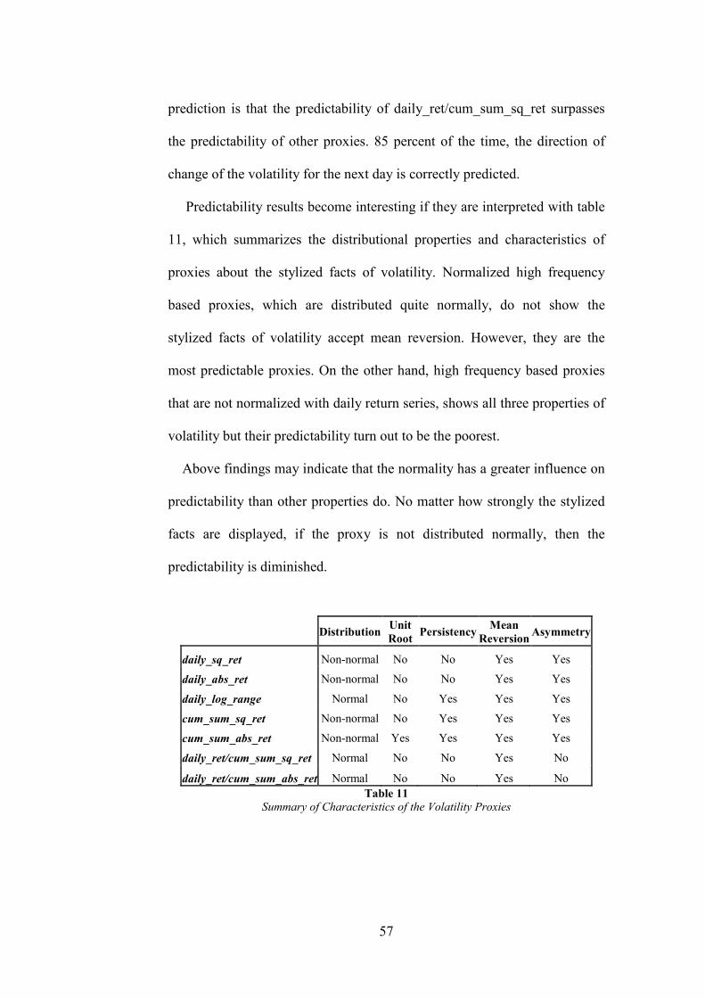
57

prediction is that the predictability of daily_ret/cum_sum_sq_ret surpasses

the predictability of other proxies. 85 percent of the time, the direction of

change of the volatility for the next day is correctly predicted.

Predictability results become interesting if they are interpreted with table

11, which summarizes the distributional properties and characteristics of

proxies about the stylized facts of volatility. Normalized high frequency

based proxies, which are distributed quite normally, do not show the

stylized facts of volatility accept mean reversion. However, they are the

most predictable proxies. On the other hand, high frequency based proxies

that are not normalized with daily return series, shows all three properties of

volatility but their predictability turn out to be the poorest.

Above findings may indicate that the normality has a greater influence on

predictability than other properties do. No matter how strongly the stylized

facts are displayed, if the proxy is not distributed normally, then the

predictability is diminished.

Distribution Unit Root Persistency Mean

Reversion Asymmetry

daily_sq_ret Non-normal No No Yes Yes

daily_abs_ret Non-normal No No Yes Yes

daily_log_range Normal No Yes Yes Yes

cum_sum_sq_ret Non-normal No Yes Yes Yes

cum_sum_abs_ret Non-normal Yes Yes Yes Yes

daily_ret/cum_sum_sq_ret Normal No No Yes No

daily_ret/cum_sum_abs_ret Normal No No Yes No Table 11

Summary of Characteristics of the Volatility Proxies

58

7. CONCLUSION AND FURTHER RESEARCH DIRECTION

The goal of this paper is to investigate the predictability of different

volatility indicators for EUR/USD exchange rate, sampled between July

2003 and February 2010, by the means of Feed Forward Neural Networks.

The effect of distributional properties and characteristics such as

persistency, mean reversion and asymmetry of these volatility proxies are

also discussed. Analyzed proxies are divided into two groups, namely low

frequency volatility proxies and proxies based on high frequency intraday

data. Low frequency proxies compose of daily square return, daily absolute

return and daily log range. Proxies that are constructed from high frequency

data are also divided into two groups. Proxies which are in the first group

are constructed by summing the intraday square returns and absolute returns

respectively. These intraday data is sampled by 10 minutes interval. The

second group of the high frequency based proxies are computed as in the

first group but they are normalized with corresponding daily returns.

According to the experimental results of direction of change prediction

for the next day, low frequency volatility proxies are more predictable than

the un normalized high frequency based volatility proxies. However, when

normalized with daily returns, high frequency based volatility proxies

become more predictable.

59

The second conclusion is about the effect of distributional feature and

stylized facts of volatility on the predictability of analyzed proxies. High

frequency-based proxies become normally distributed when they are

normalized with daily returns. These normalized series, unlike from un-

normalized ones, do not display the stylized of volatility. However, their

predictability is found to be superior. This leads us to the inference that the

distributional property may have a stronger effect on predictability than the

stylized facts do.

Despite the limitations of this thesis, I was able to differentiate the

predictability of low frequency proxies and high frequency based volatility

proxies by the means of Feed Forward Neural Network model for the

foreign currency and time period I have considered. Further work is also

needed to examine whether the derived outcomes are valid for other

currencies or not. Similarly, comparing the prediction power of other

econometric volatility models and artificial neural network structures may

help us to better understand the dynamics of volatility.

60

List of References

Andersen, T.G., Bollerslev, T., Diebold, F. X. & Labys, P. 2001, 'The

distribution of realized exchange rate volatility', Journal of American

Statistical Association, vol. 96, no. 453, pp. 42–57.

Avci, E. 2007, 'Forecasting daily and sessional returns of the ISE-100 Index

with neural network models', Dogus Universitesi Dergisi, vol. 8 pp. 128-142

Aragonés, J. R., Blanco, C. & Estévez, P. G. 2007, 'Neural network

volatility forecasts', Intelligent Systems in Accounting, Finance and

Management, vol. 15, pp. 107-121.

Bali, T. & Demirtas, O. 2008, 'Testing mean reversion in financial market

volatility: Evidence from S&P 500 index futures', Journal of Futures

Markets, vol. 28, no. 1, pp. 1-33.

Ball, C.A. & Torous, W. N. 1984, 'The maximum likelihood estimation of

security price volatility: Theory, evidence and application to option pricing',

Journal of Business, vol. 57, no. 1, pp. 97–113.

61

Bekiros, S. D. & Georgoutsos, D. A 2008, 'Direction-of-change forecasting

using a volatility-based recurrent neural network', Journal of Forecasting,

vol. 27, pp. 407-417

Black, F. 1976, 'The pricing of commodity contracts', Journal of Financial

Economics,vol. 3, pp. 167–179.

Chortareas, G., Nankervis, J. & Jiang, Y. 2007, 'Forecasting exchange rate

volatility with high frequency data: Is the euro different?'

Christie, A.A. 1982, 'The stochastic behavior of common stock variances-

value, leverage and interest rate effects', Journal of Financial Economics,

vol. 10, pp. 407–432.

Cifter, A. & Ozun, A. 2007, 'The effects of international F/X markets on

domestic currencies using wavelet networks: evidence from emerging

markets', Munich Personal RePEc Archive

Davies, P. C. 1995, Neural Network Techniques for Financial Time Series

Analysis in Virtual Trading, J. Lederman & R. A. Klein, (ed), Probus

Publishing, pp. 81-87.

http://ideas.repec.org/p/mmf/mmfc06/79.html

http://ideas.repec.org/p/mmf/mmfc06/79.html

62

Ding, Z., Granger, C. W. J. & Engle, R. F. 1993, 'A long memory property

of stock market returns and a new model', Journal of Empirical Finance,

vol. 1, pp. 83-106.

Donaldson, R.G. & Kamstra, M. 1996, 'Forecast combining with neural

networks', Journal of Forecasting, vol. 15, pp. 49–61.

Dunis, C. L. & Huang, X. 2002, ' Forecasting and trading currency

volatility: An application of recurrent neural regression and model

combination', Journal of Forecasting, vol. 21, pp. 317-354.

Fama, E.F. & Blume, M.E. 1966, 'Filter rules and stock-market trading',

Journal of Business, vol. 39, pp. 226–241.

Figlewski, S. 1997, 'Forecasting volatility', Financial Markets, Institutions

and Instruments, vol. 6, no. 1, pp. 1–88.

Franses, Ph. H. & Dick, V. D. 2000, Nonlinear Time Series Models in

Empirical Finance, Cambridge University Press, Cambridge.

Garman, M.B. & Klass, M. J. 1980, 'On the estimation of security price

volatilities from historical data', Journal of Business, vol. 53, no. 1, pp. 67–

78.

63

Gestel, V. & Tony, A. 2005, 'Linear and non-linear credit scoring by

combining logistic regression and support vector machines', Journal of

Credit Risk, vol. 1, no. 4, pp. 31-60.

Ghysels, E., Santa-Clara, P. & Valkanov, R. 2005, 'There is a risk-return

trade-off after all', Journal of Financial Economics, vol. 76, pp. 509-548.

Giles, D. 2008, 'Some properties of absolute return as a proxy for volatility',

Applied Financial Econometric Letters, Taylor and Francis Journals vol. 4,

pp. 347-350

Giles C., Lawrence S. & Tsio A. 2001, 'Noisy time series prediction using a

recurrent neural network and grammatical inference', Machine Learning,

vol. 44, no. 1/2, pp. 161-183.

Gradojevic, N. & Yang, J. 2000, Financial markets department Bank of

Canada Ottawa, Working Paper, Ontario, Canada no. K1A 0G9.

Hamid, S. A. 2004, 'Primer on using neural networks for forecasting market

variables', Working Paper no. 2004-03.

Hol, E. & Koopman, S. J. 2002, 'Forecasting the variability of stock index

returns with stochastic volatility models and implied volatility', Working

paper, Free University, Amsterdam.

http://en.wikipedia.org/wiki/Journal_of_Financial_Economics

64

Hornik, K. 1991, 'Approximation capabilities of multilayer feedforward

networks', Neural Networks, vol. 4 pp. 251-257.

Hornik, K., Stinchcombe M. & White H. 1989, 'Multilayer feedforward

networks are universal approximators', Neural Networks, vol. 2 pp. 359–

366.

Kalman, B. L, & Kwasny, S. C. 1992, 'Why Tanh? Choosing a Sigmoidal

Function', International Joint Conference on Neural Networks, Baltimore,

MD, USA

Kean, J. 1993, 'Neural Nets and Stocks', Training a Predictive System, pp.

45-47.

Kuan, C. M. & White, H. 1994, 'Artificial neural networks: An econometric

perspective', Econometric Reviews, vol. 13, no. 1, pp. 1-91.

Lawrence, J. 1994, Introduction to Neural Networks: Design, Theory, and

Applications 6th edition, Luedeking, S. (ed), California Scientific Software,

California, USA,

Mandelbrot, B 1963, 'The variation of certain speculative prices', The

Journal of Business of the University of Chicago, vol. 36, pp. 394-419.

65

Markham, I.S. & Rakes, T.R. 1998, 'The effect of size and variability of

data on the performance of neural networks and regression', Computers and

Operations Research, vol. 25, no. 4, pp. 251-263.

Masters, T. 1993, Practical Neural Network Recipes in C++, Academic

Press Inc., San Diego, CA., USA

Martens, M. & Poon, S.H. 2001, 'Returns synchronization and daily

correlation dynamics between international stock markets', Journal of

Banking and Finance, vol. 25, no. 10, pp. 1805–1827.

Martens, M. & Zein, J. 2004, 'Predicting financial volatility: High-frequency

timeseries forecasts vis-`a-vis implied volatility', Journal of Futures

Markets, vol. 24, no. 11, pp. 1005–1028.

Merton, R.C. 1980, 'On estimating expected return on the market: An

exploratory investigation', Journal of Financial Economics, vol. 8, pp. 323–

361.

Pagan, A.R. & Schwert, G. W 1990, 'Alternative models for conditional

models for conditional stock volatility', Journal of Econometrics, vol. 45,

no. 1–2, pp. 267–290.

66

Parkinson, M. 1980, 'The extreme value method of estimating the variance

of the rate of return', Journal of Business, vol. 53, pp. 61-65.

Patton, A. 2004, 'Modelling asymmetric exchange rate dependence,'

Working Papers, no.04-04, Warwick Business School

Poon, S. H. & Granger C.W. J. 2003, 'Forecasting financial market

volatility: A review', Journal of Economic Literature, vol. 41, no. 2, pp.

478–539.

Ripley, B. D. 1993, 'Statistical aspects of neural networks', Networks and

Chaos: Statistical and Probabilistic Aspects, Barndoff-Nielsen, O. E.,

Jensen, J.L. & Kendall, W.S. (eds), Chapman and Hall, London, United

Kingdom, 1993.

Rogers, L.C.G. & Satchell, S. E. 1991, 'Estimating variance from high, low

and closing prices', Annals of Applied Probability, vol. 1, pp. 504–512.

Schittenkopf, C., Dorffner, G., & Dockner, E. J. 1998, 'Volatility predictions

with mixture density networks, in ICANN 98 – Proceedings of the 8th

International Conference on artificial Neural Networks, L. Niklasson, M.

Bodén and T. Ziemka, (ed), Berlin, pp. 929-934.

http://ideas.repec.org/p/wbs/wpaper/wp04-04.html

http://ideas.repec.org/s/wbs/wpaper.html

67

Tan, C. N. W. 2000, ‘An artificial neural networks primer with financial

applications examples in financial distress predictions and foreign exchange

hybrid trading system’

Taylor, S.J. 1986, Modelling Financial Time Series, John Wiley, Chichester.

Tenti, P. 1996, 'Forecasting foreign exchange rates using recurrent neural

networks', Applied Artificial Intelligence, vol. 10, pp. 567-81.

Thomaidis, N. S. 2004, 'Efficient statistical analysis of financial time-series

using neural networks and GARCH models'

Tino, P., Schittenkopf, C. & Dorffner, G. 2000, 'Temporal pattern

recognition in noisy non-stationary time series based on quantization into

symbolic streams: Lessons learned from financial volatility trading', URL

http://citeseer.nj.nec.com/tino00temporal.html. (URL accessed on January

12, 2009).

Triacca, U. 2007, 'On the variance of the error associated to the squared

return as proxy of volatility', Applied Financial Econometric Letters, Taylor

and Francis Journals, vol. 3 pp. 255-257

Tsibouris, G. & Zeidenberg, M. 1995, Testing the Efficient Markets

Hypothesis with Gradient Descent Algorithms, Wiley, New York

http://ideas.repec.org/a/taf/apfelt/v3y2007i4p255-257.html

http://ideas.repec.org/a/taf/apfelt/v3y2007i4p255-257.html

68

Veronesi, P. 1999, 'Stock market overreaction to bad news in good times: A

rational expectations equilibrium model', Review of Financial Studies, vol.

12, pp. 975-100

White, H. 1989a, 'Connectionist nonparametric regression: Multilayer

feedforward networks can learn arbitrary mappings', Neural Networks, vol.

3, pp. 535-549.

White, H. 1989b, 'Learning in artificial neural networks: A statistical

perspective', Neural Computation, vol. 1, pp. 425-464.

Yao, J.T., Poh, H.L. & T. Jasic, 1996. 'Foreign exchange rates forecasting

with neural networks', Proceedings of the International Conference on

Neural Information Processing, Hong Kong, pp. 754-759.

Zhang, G. P. 2001, 'An investigation of neural network for linear time-series

forecasting', European Computers & Operational Research, vol.28 pp.

1183-1202.

direction of change prediction in the eur/usd … fileeur/usd exchange rate volatility using neural...

Documents