direct simulation of sounds generated by collision between …€¦ · · 2014-05-13direct...

Direct simulation of sounds generated by collision between water drop and water surface

M. Tsutahara1, S. Tajiri1, T. Miyaoka1, N. Kobata1 & H. Tanaka2 1Graduate School of Engineering, Kobe University, Japan 2Universal Shipbuilding Corporation, Japan

Abstract

In this paper, we present some applications of the finite difference lattice Boltzmann method (FDLBM) to direct simulations of fluid dynamic sound. Two-particle model is used to simulate two-phase flows, and introducing a fluid elasticity the sound propagation inside the liquid is recovered. The sounds generated by bubbles and water drop collision on the shallow water and on deep water are successfully simulated. Keywords: fluid dynamic sound, lattice Boltzmann method, two-phase flow, underwater sound，bubble, water drop.

1 Introduction

The lattice Boltzmann method [1–6] is now a very powerful tool of computational fluid dynamics (CFD). This method is different from ordinary Navier-Stokes equations based CFD methods, and is based on the particle motions. However, mostly successful model so far is for incompressible fluids, but several models for thermal compressible models have been proposed including our model [7–13]. On the other hand, this method has great advantage to simulate multi-phase flows, because the interface is automatically determined in this method without special treatment [14–17]. We propose a new model for liquids considering the elasticity of liquid, and the sound speed propagating inside the liquid is correctly realized. A simulation of a water drop colliding the water surface and sound emission is performed.

Computational Methods and Experimental Measurements XIV 71

© 2009 WIT PressWIT Transactions on Modelling and Simulation, Vol 48, www.witpress.com, ISSN 1743-355X (on-line) doi:10.2495/CMEM090071

2 Basic equations

2.1 Discrete BGK equation

The basic equation for the finite difference lattice Boltzmann method is the following discrete BGK equation

( )1k kk eqki i

i i if fc f ft xα

α τ∂ ∂

+ = − −∂ ∂

(1)

where if is the distribution function which is the number density of the particle having velocity ciα and subscripts i represents the direction of particle translation and α is the Cartesian co-ordinates. eq

if is the local equilibrium distribution function. The term on the right hand side represents the collision of particles and τ is called the single relaxation time factor. Superscript k represents gas and liquid phases, and we will use two particle model and k G= represents gas phase and k L= liquid phase, respectively. Macroscopic variables, density ρ , flow velocity u are obtained by

p pm mk k eqk

i ii i

f fρ = =∑ ∑ (2)

, ,p pm mG L G Lk eqk

i i i ik i k i

f fρ = =∑∑ ∑∑u c c (3)

where pm represents the number of the particles. The pressure for gas phase

is / 3GP ρ= .

2.2 Interface treatment

In order to obtain sharp interface for immiscible two-particle model, artificial separation techniques are sometimes introduced. In this study, phase separation or re-color technique by Latva-Kokko and Rothman [18, 19] is employed.

In this technique, an additional term is introduced to the discrete BGK equation as

( ) ( )1k kk eqk k ki i

i i i i if fc f f f ft xα

α τ∂ ∂ ′+ = − − + −∂ ∂

(5)

where kif ′ is re-distributed function calculated from the gradient of the interface.

kif ′ is given by

( )( )

( )

( )( )

( )

(0) (0)2

(0) (0)2

cos

cos

G G L eqG eqLG G Li i i i i i

G L G L

L G L eqG eqLG LLi i i i i i

G L G L

f f f f f

f f f f f

ρ ρ ρκ ϕρ ρ ρ ρ

ρ ρρ κ ϕρ ρ ρ ρ

′ = + + ++ +

′ = + − ++ +

(6a,b)

72 Computational Methods and Experimental Measurements XIV

© 2009 WIT PressWIT Transactions on Modelling and Simulation, Vol 48, www.witpress.com, ISSN 1743-355X (on-line)

κ is separation parameter to control the thickness of the diffusive (0)eqk

if is the equilibrium distribution function for velocity zero

,G Li if f′ ′ is not changed

ϕ is the angle between the gradient of the density and the particle

cos ii

i

ϕ ⋅=

⋅G cG c

(7)

( ) ( ) ( )G Li i i

iρ ρ = + − + ∑G x c x c x c (8)

2.3 Introduction of external forces

External forces are introduced to the equilibrium distribution function as an impulsive force per mass. The equilibrium distribution function

( ), ,eqk eqk ki if f t uαρ= is modified by the external force Fα as

ρ ρ→ (9) u u Fα α ατ→ + (10)

where the impulsive force includes the gravitational force in Sec. 2.4, the surface tension force in Sec.2.5, and the acceleration modification due to the density difference in Sec.2.6.

2.4 Gravitational force

The gravitational force can be introduced by expressing the force in (10) as F gα α αβδ= (11)

where gα represents the direction of the gravitational force. However, this force is not employed in this study, because some compression waves generated when the gravitational force is introduced inside the deep water described later and these waves hardly damps. Instead of introducing the gravitational force, the initial velocity of the drop is imposed, and the detail will be given in Sec.4.

2.5 Surface tension

We employ a model proposed by Gunstensen et al. [20] and Continuum Surface Force (CSF) method [21]. In CSF, the surface tension force SF is given by

ˆS σ=F Κn (12) where σ is the surface (interfacial) tension coefficient，Κ is the curvature of the interface, n̂ is the normal unit vector of the interface, and ( ) ( ) ( )ˆ =n x n x n x . The normal vector on the interface ( )n x is calculated by



where interface and considering the natural or pure diffusion. Each sum of at the collision, and then the density, the momentum and the energy are conserved. velocity and given by

( )( ) ( )( )G Lρ ρ∂ −

=∂

x xn x

x (13)

The curvature Κ is also calculated by

( ) ( )1ˆ

= − ∇ ⋅ = ⋅∇ − ∇ ⋅

nΚ n n nn n

(14)

2.6 Model for two fluids with large density difference

He et al. [22] have proposed a large density difference fluid model up to about 40, and Inamuro et al. [23] have proposed a model with density difference up to 1000. But the fluid of liquid phase is completely incompressible in Inamuro’s model, and the sound in liquid phase cannot be simulated with this model. Therefore we will propose a novel model for two-phase flows with large density difference. The density difference is realized by changing the acceleration, and this effect is also introduced to the model by impulsive force for each particle

2 21 1in

P Pm m

µ µρ ρ ρ ρ

′ ′ ∂ ∂′= − + = − − + ∇ + − + ∇ ∂ ∂ F a a u u

x x (15)

where P′ is the effective pressure, and a is the acceleration to cancel the original force term, ′a is newly introduced acceleration due to the density and the viscosity of considering fluid. m represents an averaged density and µ′ is an averaged viscosity

,

,

k k

k G Lk

k G L

mm

ρ

ρ=

=

=∑∑

,

,

k k

k G Lk

k G L

µ ρµ

ρ=

=

′ =∑∑

(16a,b)

The density ratio of the two fluids is given as /L Gm m , and in case of water and air, it is about 800, and the ratio of viscosity is about 70 and they change continuously across the interface.

2.7 Compressibility of liquid

A simple model of bulk elasticity is introduced to consider the compressibility of the liquid as

0 0( )P P β ρ ρ′ = + − (17) where β is a parameter to control the elasticity and corresponds the bulk modulus of elasticity and 0P is a reference pressure and 0ρ is a reference density and is fixed to unity in this study. In liquid phase, we do not consider the temperature change. The sound speed of the liquid phase is given as

LLs L

Pcmβ

ρ′∆

= =∆

(18)



2.8 Two-dimensional 9 velocity model

In this study, two-dimensional 9-velocity (D2Q9) model [1–6] is used, whose equilibrium distribution function is given by

2, , ,

9 31 32 2

eqi i i i if u c u u c c uα α α β α βω ρ = + + −

(19)

where 0 1 4 5 84 9, 1 9, 1 36ω ω ω− −= = = (20)

The velocity set is shown in Fig.1 and expressed as ( )

( ) ( )( )( ) ( )( )

0,0 0

cos 1 2 ,sin 1 2 1 4

2 cos 9 2 2 ,sin 9 2 2 5 8

i

i

i

for i

i i for i

i i for i

π π

π π

= =

= − − = −

= − − = −

c

c

c

　

(21)

The sound velocity in gas phase is 1/ 3Gsc = by this model.

The scheme for calculation is the third order upwind scheme (UTOPIA) for space and the second order Runge-Kutta method for time integral.

3 Underwater sound augmented by air bubbles

As a preliminary test, we briefly describe the simulation on the underwater sound augmented by air bubbles. The initial condition is shown in Fig.1. A circular cylinder is set in a uniform flow of water, and three bubbles approach the cylinder. The computation parameters are as follows. The number of grid is 251×154 . The flow velocity is 0.2U = (normalized by the particle velocity given in (21)), and the kinetic viscosity of water is 0.01ν = . The separation parameter and the surface tension are 2.0κ = and 0.00001σ = , respectively. The ratio of gas-liquid densities is 1:800 (air and water) and liquid bulk elasticity is 6400Lβ = . The non-dimensional time is defined by * /T tU D= .

Figure 1: Initial position of circular cylinder and bubbles.

Figure 2(a) shows the bubble position and sound pressure field around the cylinder. Aeolian tone can be detected, but in this scale the pattern cannot be shown. A circular disturbance is that occurs at the early stage when the flow suddenly starts. Figure 2(b) shows that when the bubbles are stretched, strong



sound is emitted, and the bubbles also produce strong dipole-like sound when they are involved in the Karmann vortices (Fig.2(c) and (d)). The direction of the dipole is perpendicular to the flow unlike Aeolian tones in which the direction is on the flow direction.

(a) * 62T = (b) * 64T =

(c) * 66T = (d) * 68T =

Figure 2: Bubble position and underwater sound.

4 Sound generated by a water drop colliding with a shallow water surface

The sound generated by a water drop colliding against the water surface is a very well-known sound, and intensive studies have been done [24, 25]. In this section, we calculated the sound generated by collision of a water drop to shallow water using the above mentioned model. The reason why we chose this problem is that the results, such as splash shape except sound, can be compared with other simulation results. In this calculation, we did not impose the gravitational force, because some internal compression waves are generated just after the gravitational force is imposed. Instead, the initial velocity was imposed as shown in Fig. 3. The parameters of the calculation are given as follows. The number of grids is 503 401× and the minimum grid size is 52 10−× . Time increment is set 62 10−× . The density ratio / 1000L Gm m = , kinematic viscosity of gas 61 10Gν

−= × , and the bulk elastic modulus of liquid is 6400. The phase separation coefficient 0.9κ = , the surface tension coefficient 71 10σ −= × , the droplet diameter 32 10D −= × , the water depth 0.075fD D= , and the initial

velocity of the droplet 0.02U = . It should be noted here that these parameters are all non-dimensional values based on the minimum particle speed 1=c , the

reference time 1t = , and the reference length / 1t =c .



UD

Df

Liquid dropletGas

Calculation domain

Non-slip wall

Mirror boundary condition

UD

Df

Liquid dropletGas

Calculation domain

Non-slip wall

Mirror boundary condition

xzy xzy

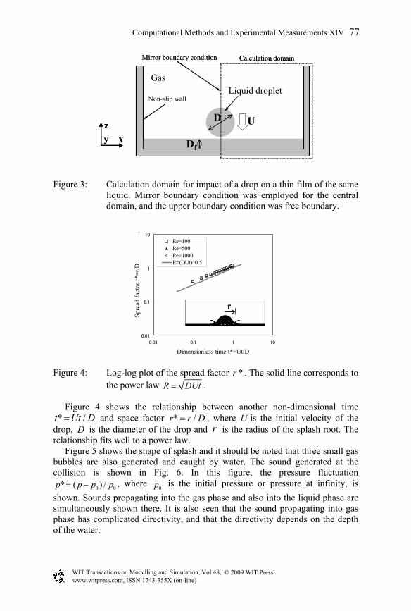
Figure 3: Calculation domain for impact of a drop on a thin film of the same liquid. Mirror boundary condition was employed for the central domain, and the upper boundary condition was free boundary.

0.01

0.1

1

10

0.01 0.1 1 10

Dimensionless time t*=Ut/D

Spre

ad fa

ctor

r*=r

/D

.

Re=100Re=500Re=1000R=(DUt)^0.5

rrr

Figure 4: Log-log plot of the spread factor *r . The solid line corresponds to the power law R DUt= .

Figure 4 shows the relationship between another non-dimensional time * /t Ut D= and space factor * /r r D= , where U is the initial velocity of the

drop, D is the diameter of the drop and r is the radius of the splash root. The relationship fits well to a power law. Figure 5 shows the shape of splash and it should be noted that three small gas bubbles are also generated and caught by water. The sound generated at the collision is shown in Fig. 6. In this figure, the pressure fluctuation

0 0* ( ) /p p p p= − , where 0p is the initial pressure or pressure at infinity, is

shown. Sounds propagating into the gas phase and also into the liquid phase are simultaneously shown there. It is also seen that the sound propagating into gas phase has complicated directivity, and that the directivity depends on the depth of the water.



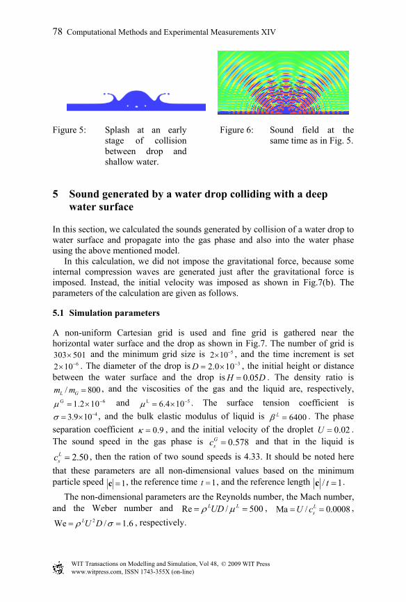
Figure 5: Splash at an early stage of collision between drop and shallow water.

Figure 6: Sound field at the same time as in Fig. 5.

5 Sound generated by a water drop colliding with a deep water surface

In this section, we calculated the sounds generated by collision of a water drop to water surface and propagate into the gas phase and also into the water phase using the above mentioned model. In this calculation, we did not impose the gravitational force, because some internal compression waves are generated just after the gravitational force is imposed. Instead, the initial velocity was imposed as shown in Fig.7(b). The parameters of the calculation are given as follows.

5.1 Simulation parameters

A non-uniform Cartesian grid is used and fine grid is gathered near the horizontal water surface and the drop as shown in Fig.7. The number of grid is 303 501× and the minimum grid size is 52 10−× , and the time increment is set

62 10−× . The diameter of the drop is 32.0 10D −= × , the initial height or distance between the water surface and the drop is 0.05H D= . The density ratio is

/ 800L Gm m = , and the viscosities of the gas and the liquid are, respectively, G 61.2 10µ −= × and L 56.4 10µ −= × . The surface tension coefficient is

43.9 10σ −= × , and the bulk elastic modulus of liquid is 6400Lβ = . The phase separation coefficient 0.9κ = , and the initial velocity of the droplet 0.02U = . The sound speed in the gas phase is 0.578G

sc = and that in the liquid is

2.50Lsc = , then the ration of two sound speeds is 4.33. It should be noted here

that these parameters are all non-dimensional values based on the minimum particle speed 1=c , the reference time 1t = , and the reference length / 1t =c . The non-dimensional parameters are the Reynolds number, the Mach number, and the Weber number and Re / 500L LUDρ µ= = , Ma / 0.0008L

sU c= = , 2We / 1.6LU Dρ σ= = , respectively.



(a) Grid system in a half domain (b) Initial position of the drop

Figure 7: Grid system near the drop and water surface and initial position of the drop. Mirror boundary condition was employed for the central domain, and the upper boundary condition is free boundary.

Figure 8: Sounds emitted into gas phase and liquid phase.

5.2 Sounds propagating in gas and liquid phases

The sounds propagating into the gas phase and liquid phase in very early stage of collision are shown in Fig.8. The sound in the gas phase is generated first as the drop moves suddenly and then generated at the collision of the drop against the water surface. On the other hand, under water sound is generated at the collision and is seen to propagate about 4 times faster than sound propagating into the gas phase. It is noted here that there appears a sound pattern inside the drop, and the sound originaly generated at the collision plane (horizontal palne) propagates upward to inside the drop and downward to the deep water. The sound goes up and reflects at the surface of the drop and goes downward again. Some of that sound passes through the neck formed by contact of the drop and water surface and goes out to the deep water and the other reflects and goes back to the drop.



The reflection continues and the sound is emmitted into the water in groups. In Fig.6, two groups are shown. We shall discuss this phenomenon later. The directivility of the sound propagation is shown in Fig.9, which is calculated by taking sound pressure data at points shown in the left figure in Fig.9 and taking the maximum pressure fluctuation

max min* *P p p∆ = − . In the gas phase, the directivility seems complicated and strong directivility is seen in the direction of 30 degrees from the horizontal surface. This sound is generated by the splash. In the liquid phase, the directivility is dipole-like and this has been reported in the rain-fall sounds.

Impact point

Liquid

Gas

0 0.005 0.01-0.01

-0.0075

-0.005

-0.0025

0

0.0025

0.005

0.0075

0.01

Norm

ali

zed

dis

tance f

rom

im

pact

poin

t r*

=r/

c

Normalized distance from impact point r*=r/c

Sampling point of pressure fluctuation

Impact point

Liquid

Gas

0 0.005 0.01-0.01

-0.0075

-0.005

-0.0025

0

0.0025

0.005

0.0075

0.01

Norm

ali

zed

dis

tance f

rom

im

pact

poin

t r*

=r/

c

Normalized distance from impact point r*=r/c

Sampling point of pressure fluctuation

-20

-15

-10

-5

0

5

10

15

20

No

rmal

ized

am

pli

tud

e o

f p

ress

ure

flu

ctu

atio

n

P*

f=|P

*f,

max

-P*

f,m

in| [

10

-7]

90[deg]

-90[deg]

45[deg]

-45[deg]

0[deg]

-20

-15

-10

-5

0

5

10

15

20

No

rmal

ized

am

pli

tud

e o

f p

ress

ure

flu

ctu

atio

n

P*

f=|P

*f,

max

-P*

f,m

in| [

10

-7]

90[deg]

-90[deg]

45[deg]

-45[deg]

0[deg]

Figure 9: Observing points and directivity of sound.

6 Conclusions

A two-phase flow model of the finite difference lattice Boltzmann method with large density difference and including the elasticity of liquid is proposed. Direct simulations of aerodynamic sound and underwater sound are successively performed, especially the sound generated on interfaces between gas and liquid.

References

[1] Qian, Y.H., Succi, S. and Orszag, S.A., Recent Advances in Lattice Boltzmann Computing, Ann. Rev. of Comp. Phy. III, D. Stauffer ed. World Scientific, pp.195-242, 1995.

[2] Rothman, D.H. and Zalenski, S., Lattice-Gas Cellular Automata, Cambridge U.P., 1997.

[3] Chopard, B.. and Droz, M., Cellular Automata Modeling of Physical Systems, Cambridge University Press, 1998.



[4] Chen, S. and Doolen, G.D., Lattice Boltzmann method for fluid flows, Ann. Rev. Fluid Mech., Ann. Rev. Inc. pp.329-364, 1998.

[5] Wolf-Gladrow, D.A., Lattice-Gas Cellular Automata and Lattice Boltzmann Models, Lecture Notes in Mathematics, Springer, 2000.

[6] Succi, S., The lattice Boltzmann Equation for Fluid Dynamics and Beyond, Oxford, 2001.

[7] Alexander, F.J. et al., Lattice Boltzmann thermodynamics, Phys. Rev. E, 47 R2249-R2252, 1993.

[8] Chen, Y., et al., Thermal lattice Bhatanagar Gross Knook model without nonlinear deviations in macrodynamic equations, Phys. Rev. E, 50, pp.2776-2283, 1994.

[9] Takada, N. and Tsutahara M., Proposal of Lattice BGK model with internal degrees of freedom in lattice Boltzmann method, Transaction of JSME B， 65-629, pp.92-99, 1999 (in Japanese).

[10] McNamara, G.R., et al., Stabilization of thermal lattice Boltzmann models, J. Stat. Phys., 81(1/2), pp. 395-408, 1995.

[11] Kataoka, T. and Tsutahara, T., Lattice Boltzmann model for the compressible Navier-Stokes equations with flexible specific-heat ratio, Phys. Rev. E, 67, pp.036306-1-4, 2004.

[12] Watari, M. and Tsutahara, T., Two-dimensional thermal model of the finite-difference lattice Boltzmann method with high spatial isotropy, Phys. Rev. E, 69, pp.035701-1-7, 2004.

[13] Tsutahara M, Takada N, Kataoka T, Lattice gas and lattice Boltzmann methods, Corona-sha, (in Japanese) 1999.

[14] Swift, M.R., Orlandini, E., Osborn, W.R., and Yeomans, J.M., Lattice Boltzmann simulations of liquid-gas and binary-fluid systems. Phys. Rev. E 54, pp.5041-5052, 1996.

[15] Swift, M.R., Osborn, W.R., and Yeomans, J.M., Lattice Boltzmann simulation of non-ideal fluids. Phys. Rev. Lett. 75, pp.830-833, 1995.

[16] Shan, X. and Chen, H., Lattice Boltzmann model for simulating fows with multiple phases and components. Phys. Rev. E 47, pp.1815-1819, 1993.

[17] Shan, X. and Chen, H. Simulation of non-ideal gases and liquid-gas phase-transitions by the lattice Boltzmann-equation. Phys. Rev. E 49, pp.2941-2948, 1994.

[18] Latva-Kokko, M., Rothman, D. H., Diffusion properties of gradient -based lattice Boltzmann models of immiscible fluids, Physical Review E, Vol.71, 056702, 2005.

[19] Latva-Kokko, M., Rothman, D. H., Static contact angle in lattice Boltzmann models of immiscible fluids, Physical Review E, Vol.72, 046701, 2005.

[20] Gunstensen, A. K., Rothman, D. H., Zaleski, S. Zanetti, G., Lattice Boltzmann model of immiscible fluid, Physical Review A, Vol.43, 4320-4327, 1991.

[21] Brackbill, J. U., Kothe, D. B., Zemach, C., A continuum method for modeling surface tension, Journal of Computational Physics, Vol.100, 335-354, 1992.



[22] He X., Chen S., and Zhang R., A lattice Boltzmann Scheme for Incompressible Multiphase Flow and Its Application in Simulation of Rayleigh-Taylor Instability, J. Computational Physics 152, pp.642-663, 1999.

[23] Inamuro T., Ogata T., Tajima S. and Konishi N., A lattice Boltzmann method of incompressible two-phase flows with large density differences, J. Computational Physics 198, pp.628-644, 2004.

[24] Pumphrey, H. C., Crum L.A., Bjomo, L., Underwater sound produced by individual drop impacts and rainfall, Journal of Acoustical Society of America 85(4), 1518-1526, 1989.

[25] Prospeeretti A., Ogus H. N., The impact of drops on liquid surface and the underwater noise of rain, Ann. Rev. Fluid Mech., 25, pp.577-602, 1993.



direct simulation of sounds generated by collision between …€¦ · · 2014-05-13direct...

Documents