direct marketing in duopolistic wholesale market
TRANSCRIPT

Direct Marketing in Duopolistic Wholesale Market
Tomomichi Mizuno∗
Graduate School of Economics, Kobe University
2-1 Rokkodai-cho, Nada-ku, Kobe-City, Hyogo 657-8501, Japan.
E-mail: [email protected]
October 30, 2008
Abstract
Many manufacturers sell their products directly to consumers using catalogues, the internet,
or their own stores. Since direct marketing is the method of selling products not through
retailers, we expect a relationship between direct marketing and competition in a retail
market. This paper studies a manufacturer’s choice whether to sell directly in the presence
of a rival manufacturer that has the same choice. We consider a game where manufacturers
decide whether to set up sites (e.g., websites or physical stores) where consumers can buy
their products directly. After the decision, manufacturers also choose the amount to sell to
retailers. Retailers and the manufacturers that have direct-sales sites then choose the amount
to sell to consumers. We show that competition in the retail market may prevent direct
marketing. Then, an increase in the number of retailers raises the profit of retailers, but
reduces social welfare. Notably, social welfare is larger when a retail market is monopoly than
when a perfectly competitive market. Therefore, we provide a justification for regulation of
retail markets.
JEL classification numbers: L13, L20
Key words: direct marketing; successive oligopoly; Cournot competition
∗I am grateful for the encouragement and helpful comments of Takashi Yanagawa, Hiroyuki Adachi, JunichiroIshida, Shingo Ishiguro, Noriaki Matsushima, Eiichi Miyagawa, Toshiji Miyakawa, Hideo Owan, Takashi Shimizu,and seminar participants at Osaka Prefecture University and Kobe University. The research for this paper wasfinnancially supported in part by the Kobe University CDAMS. Needless to say, all remaining errors are mine.
1

1 Introduction
Nowadays, manufacturers sell many products (for instance, personal computers, furniture and
clothes) not only to retailers but also to consumers using the internet or their own stores. That
is, manufacturers encroach on the retail market by using direct marketing.1 Examples can
be found in food industries.2 During the period from 1997 to 2002, the value of agricultural
products sold directly to individuals for human consumption increases from $591,820,000 to
$812,204,000 (U.S. Department of Agriculture, 2004).
Since direct marketing connects manufacturers to consumers directly, a decision of whether
to use direct marketing depends on a competition among retailers. If there are few retailers,
the retailers resell good at a high markup. Then, since the gain from the wholesale market is
small, manufacturers will sell their products to consumer directly. On the other hand, if the
retail market is perfectly competitive, the manufacturers will not sell directly.
When the the marginal cost of direct sales is zero, the monopolistic manufacturer certainly
encroaches on the retail market, since it gains monopoly profit. However, if there are two man-
ufacturers, it is not necessarilly the case that the manufacturers certainly encroach on the retail
market. Since encroaching manufacturers also care about the profit from the retail market,
to make the retailers’ share small and obtain large share in the retail market, the encroaching
manufacturers have an incentive to increase wholesale price. Then, the encroaching manufac-
turers sell a small amount of the product. In other words, the decision not to encroach on the
retail market makes the non-encroaching manufacturer sell the larger amount of product to the
retailers. Then, the non-encroaching manufacturer gains the larger profit from the wholesale
market than the encroaching manufacturer, but losses the profit from the retail market. Hence,
there is a trade-off between encroaching on the retail market and non-encroaching.
The present paper studies this issue by using the following model (see Figure 1). There are
two manufacturers and multiple retailers. Each manufacturer chooses whether to sell to both
retailers and consumers or to sell only to retailers. Given a sales channel, manufacturers choose
the amount of products to sell to the wholesale market. The wholesale price is determined
1 For impacts of e-commerce on food marketing, see Baourakis et al. (2002).
2 For the food market structure, see Barkema et al. (1991), Rogers (2001), Sexton (2000), and Wrigley (2001).
2

to clear the market. Then, manufacturers and retailers choose the amount of products sold to
consumers. The manufacturer’s marginal costs of direct and indirect sales are zero. The retailers
buy the product from the wholesale market, and sell it to consumers with no additional cost.
We show that when there are six retailers, one manufacturer sells only through the indirect
sales channel, while the other sells only through the direct sales channel. When the number
of retailers exceeds 7, no manufacturers sells directly even though the marginal cost of direct
sales is zero. If an increase in the number of retailers decreases the number of encroaching
manufacturers, the profit of retailers increases. When there are five retailers, social welfare is
maximized. Especially, social welfare in the case in which the retail market is monopoly is larger
than that in the case in which the retail market is perfectly competitive. We also consider that
the retailers can create their divisions, and show that manufacturers’ encroachment is always
deterred. By extending the model to include many manufacturers, we provide the number of
retailers such that social welfare is maximized given the number of manufacturers.
Arya et al. (2007) investigate a monopolistic manufacturer’s encroachment by using direct
marketing. When the manufacturer decides whether to sell its product directly, it compare the
cost of direct marketing with that of double marginalization. If the marginal cost of direct sales is
small, the monopolistic manufacturer encroaches. Since the manufacturer’s encroachment makes
the retail marke more competitive, it reduces the wholesale price in order not to decrease the
sales in the wholesale market. Then, the encroachment may be beneficial for retailers. According
to Arya et al. (2007), when encroachment arises, the manufacturer and consumers both benefit
from encroachment. If the marginal cost of direct sales in some range, the retailers also gain
from the encroachment. That is, social welfare may increase by manufacturer’s encroachment.
Lahiri and Ono (1988) show if less efficient firms enter the market, social welfare may
decrease. When a less efficient firm enters the market, efficient firms’ production decreases
and the inefficient firm’ production increases. Hence, since the average efficiency of production
decreases, social welfare may decrease. In our model, when encroaching manufacturers exit the
retail market, sales through retailers increase. That is, good is sold through the channel with
double marginalization but through without it. The channel through retailers is socially costly.
Hence, since encroaching manufacturers may exit, an increase in the number of retailers may
decrease social welfare.
3
While Lahiri and Ono (1988) focus on firms’ technologies, we look into logistics (direct and
indirect sales channels). We show that even if there are no differences of technology among
firms, an increase in the number of retailers reduces social welfare. The driving force of this
result is a vertical relationship that is not considered in Lahiri and Ono (1988).
There are some papers that consider direct marketing. Sibley and Weisman (1998) consider
the entry of an upstream monopolist into downstream markets and show that the upstream
monopolist has an incentive to reduce the costs of its downstream competitors.3 Chiang et al.
(2003) use a quality differentiation model (see Gabszewicz and Thisse, 1979, 1980 and Shaked
and Sutton, 1982, 1983) and show that direct marketing may not always be harmful for retailers.
However, these studies do not treat imperfect competition among manufacturers.
Over the past two decades, several papers have been devoted to successive oligopoly. Salinger
(1988) considers vertical integration in a successive Cournot market. Salinger (1988) shows
that the vertically merged firm increases its final good output and withdraws from the whole-
sale market. However, Salinger (1988) does not consider supplier encroachments. Following
Salinger (1988), some papers discuss successive oligopoly markets but do not consider supplier
encroachments.4
In the literature of successive oligopoly, Buehler and Schmutzler (2005) consider vertical
integration in successive oligopoly and show that only some of the firms integrate. Lin (2006)
considers spin-offs of input divisions and shows that spin-offs occur if and only if the number
of downstream firms exceeds a threshold level. However, these papers do not consider supplier
encroachments.
The remainder of this paper is organized as follows. Section 2 presents the model. Section
3 calculates the equilibrium. Section 4 studies the effect of the number of the retailers on the
equilibrium outcomes. Section 5 considers divisionalization problem. Section 6 allows that there
3 For raising rivals’ costs, also see Salop and Scheffman (1983).
4 Ziss (2005) analyzes a horizontal merger in successive oligopoly and shows that a merger at the merging and
non-merging stages reduces social welfare and the size of the reduction depends on the level of concentration of
industries. Matsushima (2006) considers industry profits in a vertical relationship and shows that the industry
profits may increase with the number of downstream firms. Like Salinger (1988) and Matsushima (2006), this
present study analyzes a successive Cournot model; however, unlike this study, they do not consider supplier
encroachments.
4

are many manufacturers. Section 7 concludes.
2 Model
This paper considers a vertical relationship in a homogeneous good market along with a three-
stage game. There exist n(≥ 1) retailers and two manufacturers. At stage one, each manufac-
turer simultaneously decides to encroach on the retail market (E) or not (N). At stage two,
each manufacturer simultaneously produces a homogeneous good at zero marginal cost and sells
it to the retailers. We call these sales indirect sales. This paper assumes Cournot competition in
the wholesale market. Let w denote the equilibrium wholesale price. The price w is determined
so that the aggregate amount of the good produced by manufacturers is equal to the aggregate
amount of the products sold to consumers by retailers (Salinger, 1988). At stage three, each
retailer simultaneously purchases the good from manufacturers and sells them to consumers at
zero marginal cost, given the equilibrium wholesale price. In the same way, each manufacturer
simultaneously sells the homogeneous products to the consumers at zero marginal cost. That
is, in the stage three, each retailer and manufacturer simultaneously decides the amount of
sales. We call the manufacturer’s sales to consumers direct sales. This study assumes Cournot
competition also in the retail market. To summarize, this study considers the following model.
Stage 1: Each manufacturer simultaneously chooses encroachment on the retail market (E) or no-
encroachment (N).
Stage 2: Each manufacturer simultaneously chooses the amount of the indirect sales. Given the
aggregate supply of the products, the wholesale price w is determined by the derived
inverse demand function for the product.
Stage 3: All retailers and manufacturers observe the wholesale price, and each retailer and manu-
facturer simultaneously chooses the amount of the product sold to consumers.
The market inverse demand function is given by P = a−bX, where a is constant and a > 0.
Let P be the price at which the retailers sell the product. Let X be the aggregate amount of the
product sold to consumers. Let qj be the amount of the product produced by manufacturer j at
5
stage two. Then, the aggregate supply of the products produced by manufacturers to retailers
is Q = q1 + q2. Let xi be the amount of the product sold by retailer i to consumers. Let dj be
the amount of the product sold directly by manufacturer j to consumers. Then, the aggregate
amount of the product sold to consumers is X = d1 + d2 +∑n
i=1 xi. The profit of manufacturer
j is
πMj =
[a− b
(d1 + d2 +
n∑
i=1
xi
)]dj + wqj . (1)
The profit of retailer i is
πRi =
[a− b
(d1 + d2 +
n∑
i=1
xi
)− w
]xi. (2)
This study assumes the complete information. The model is solved by backward induction.
Only pure strategies are considered throughout this paper.
3 Calculating Equilibrium
3.1 The no-encroachment setting
First, we consider the no-encroachment setting in which all manufacturers cannot directly sell
products to consumers. That is, in stage one, all manufacturers choose not to encroach on the
retail market. In other words, all manufacturers choose zero direct sales: d1 = d2 = 0. Then,
in stage three, retailer i’s profit is
πRi =
(a− b
n∑
i=1
xi
)xi. (3)
Then, the first-order condition leads to
xi =a− w
b(1 + n). (4)
Adding up the quations (i = 1, . . . , n) and putting∑n
i=1 xi = Q(= q1 +q2) into it, we obtain
the derived demand for input:
w = a− b(1 + n)(q1 + q2)n
. (5)
6

Substituting (5) and dj = 0 into (24), the profit of manufacturer j can be rewritten as follows:
πMj =[a− b(1 + n)(q1 + q2)
n
]qj . (6)
Then, the first-order condition leads to
xNNi =
2a
3b(1 + n), XNN =
2an
3b(1 + n), PNN =
a(3 + n)3(1 + n)
, qNNj =
an
3b(1 + n), wNN =
a
3, (7)
πNNMj =
a2n
9b(1 + n), πNN
Ri =4a2
9b(1 + n)2, (8)
where the superscript NN denotes the no-encroachment setting.
3.2 One firm’s encroachment setting
Here, we consider the case where only one manufacturer can directly sell the products to con-
sumers, that is, in stage one, one manufacturer decides to encroach on the retail market, but
the other chooses no-encroachment. Without loss of generality, we assume that manufacturer
1 chooses encroachment (E) and manufacturer 2 chooses no-encroachment (N). Then, d2 = 0.
From (24) and (25), the first-order conditions in stage three lead to
xi =a− 2w
b(2 + n), d1 =
a + nw
b(2 + n). (9)
Adding up the first equations (i = 1, . . . , n) in (9) and putting∑n
i=1 xi = Q into it, we
obtain the derived demand for input:
w =a
2− b(2 + n)(q1 + q2)
2n. (10)
We substitute d2 = 0, (9), and (10) into the manufacturer 1’s profit (24), and then differentiate
with respect to q1. We obtain
∂πMj
∂q1= − b
2n(4q1 + nq1 + 2q2) . (11)
Hence, the encroaching manufacturer 1 produces zero output for the retailers (q1 = 0). We
substitute d2 = 0, q1 = 0, (9), and (10) into manufacturer 2’s profit (24), then the first-order
7

condition for manufacturer 2 in stage two leads to
xENi = xNE
i =a
2b(2 + n), dEN
1 = dNE2 =
a(4 + n)4b(2 + n)
, (12)
qEN1 = qNE
2 = 0, qEN2 = qNE
1 =an
2b(2 + n), (13)
XEN = XNE =a(4 + 3n)4b(2 + n)
, wEN = wNE =a
4, PEN = PNE =
a(4 + n)4(2 + n)
, (14)
πENM1 = πNE
M2 =a2(4 + n)2
16b(2 + n)2, πEN
M2 = πNEM1 =
a2n
8b(2 + n), πEN
Ri = πNERi =
a2
4b(2 + n)2, (15)
where the superscript EN denotes that manufacturer 1 encroaches on the retail market, but
manufacturer 2 does not. Similarly, when manufacturer 2 encroaches on the retail market, but
manufacturer 1 does not, we use the superscript NE.
3.3 Full encroachment setting
Here, we consider the case where all manufacturers can directly sell the products to consumers.
That is, in stage one, all manufacturers decide to encroach on the retail market. From (24) and
(25), the first-order conditions in stage three lead to
xi =a− 3w
b(3 + n), dj =
a + nw
b(3 + n). (16)
Adding up the first equation in (16) and putting∑n
i=1 xi = Q into it, we obtain the derived
demand for input:
w =a
3− b(3 + n)(q1 + q2)
3n. (17)
We substitute (16) and (17) into (24), then the first-order condition for manufacturer j in stage
2 leads to
xEEi =
2a
b(27 + 5n), qEE
j =an
b(27 + 5n), dEE
i =a(9 + n)
b(27 + 5n), (18)
XEE =2a(9 + 2n)b(27 + 5n)
, PEE =a(9 + n)27 + 5n
, wEE a(7 + n)27 + 5n
, (19)
πEEMj =
a2(81 + 25n + 2n2)b(27 + 5n)2
, πEERi =
4a2
b(27 + 5n)2, (20)
where the superscript EE denotes the encroachment setting. If c/a ≥ (9 + n)/(9 + 7n), then
8

dEEj = 0. Hence, the outcomes are the same as that in the no-encroachment setting.
3.4 Encroachment decisions
Here, to derive equilibrium strategies in stage one, we compare the equilibrium profits in stage
two. See the following 2× 2 matrix (Table 1). The payoff in each cell is depicted as follows:
• πNNM1 = πNN
M2 is in (8)
• πENM1 = πNE
M2 is in (15)
• πNEM1 = πEN
M2 is in (15)
• πEEM1 = πEE
M2 is in (20)
Table 1 is here.
Since manufacturers are symmetric, it is sufficient to consider the signs of πEEM1 − πNE
M1 and
πENM1 − πNN
M1 . After tedious calculations, we have the following result:
Proposition 1 The first-stage outcome is (E, E) if n < 5.906; (N, E) and (E, N) if 5.906 ≥n ≥ 6.355; (N, N) if n > 6.355.
Proof. See Appendix.
From Proposition 1, for n ≥ 7, encroachment does not arise. This result differs from
Arya et al. (2007), who show that for any number of retailers, monopolistic manufacturer’s
encroachment does arise, if the marginal cost of direct sales is sufficiently small. The difference
arises for the following reason. When the wholesale market is monopoly, the monopolistic
manufacturer should sell to consumers directly since the manufacturer can gain the monopoly
profit. When the wholesale market is duopoly, the commitment not to sell to consumers directly
has a benefit. Even if the marginal cost of direct sale is zero, the manufacturers decide not to
encroach, when the benefit from the commitment exceeds the cost.
9

To obtain the intuition behind Proposition 1, we explain the benefit of the commitment not
to encroach on the retail market. From (24), the first-order condition in stage two is
∂πMj
∂qj= (a− bX)
∂dj
∂w
∂w
∂qj− bdj
∂X
∂w
∂w
∂qj+ qj
∂w
∂qj+ w = 0. (21)
In (21), the first and second terms represent the effect on the profit from the retail market. The
third and forth terms represent the effect on the profit from the wholesale market.
An increasing the output decreases the equilibrium whoelsale price. The more competitive
the retail market is, the more elastic the retail demand. Hence, from (5), (10), and (17),
we have ∂wNN/∂qj < wEN/∂qj < wEE/∂qj < 0. In our setting, from (5), (10), and (17),
∂wNN/∂qj , wEN/∂qj and wEE/∂qj are constant. From (12) and (18), since an increase in the
wholesale price increases the retailers’ marginal cost, retailers’ sales decrease (∂xi/∂w < 0) and
manufacturers’ direct sales increase (∂dj/∂w > 0). Since an increase in the retailer’s marginal
cost w leads the retail market to become less competitive, the aggregate output in the retail
market X decreases. That is, ∂X/∂w < 0. Therefore, the first, second and third terms are
negative.
When manufacturers do not encroach on the retail market, the first and second term in
(21) is zero, since dj = 0. Hence, the encroaching manufacturer’s output for the wholesale
market qj is smaller than the non-encroaching manufacturer’s output, since the first and second
terms are negative. We call the effect on the equilibrium output the commitment effect. Since
∂wNN/∂qj < wEN/∂qj < wEE/∂qj < 0, the third term in (21) makes the non-encroaching
manufacturer’s output for the wholesale market small. We call this effect on the equilibrium
output the competition effect. In our model, the commitment effect dominates the competition
effect. Therefore, the decision not to encroach means a commitment to produce larger output
in the wholesale market.
When a manufacturer changes the action from encroaching (E) to no encroaching (N), the
cost is loss of profit from the retail market and the benefit is larger sales in the wholesale market.
When the competitor encroaches, the benefit is larger and the cost is smaller than when it does
not. The benefit increases with the number of retailers (n) since the retailers’ demand for the
product is larger. The cost decreases with n, since direct sales are smaller when there are many
competitors in the retail market. Figure 2 summarizes the above discussion.
10

Figure 2 is here.
In Figure 2, there are four solid lines. When the competitor’s action is k (k ∈ E, N), the
line Benefitk means the benefit from changing the action from E to N , and the line Costk
means the cost from the change. We divide the set n into three ranges: [0, 5.906), [5.906, 6.355],
and (6.355,∞). First, if n is small, that is n ∈ [0, 5.906), regardless of the competitor’s action
(E or N), the costs are larger than the benefits. Thus, manufacturers do not change their
action from E to N . Hence, the equilibrium action is (E, E). Second, if n is large, that is
n ∈ (6.355,∞), regardless of the competitor’s action, the benefits are larger than the costs.
Hence, the equilibrium action is (N, N). Therefore, when n ≥ 7, no manufacturers encroach
on the retail market, even if marginal cost c is zero. Finally, if n is not so large, that is
n ∈ [5.906, 6.355], BenefitE is larger than CostE , but BenefitN is smaller than CostN . Hence,
the manufacturer encroaches if the competitor does not encroach, but not otherwise. Therefore,
the equilibrium actions are (E, N) and (N, E).
4 Comparative Statics
4.1 The profit of retailers
Ordinary, an increase in the number of retailers decrease each retailer’s profit. In this subsection,
we show that the retailer’s profit is not maximized when the retail market is monopoly.
We describe a relationship between the number of retailers and the profit of retailer. From
Proposition 1, and (8), (15) and (20), bπ∗Ri/a2 is drawn in Figure 3, where the superscript ∗denotes the equilibrium outcome in stage one.
Figure 3 is here.
In Figure 3, there are three intervals, that is, [0, 5.906), [5.906, 6.355], and (6.355,∞). If
the number of retailers increase from 5 to 6 or from 6 to 7, the retailer’s profit increases. This
is because when the number of retailers increases from 5 to 6 or from 6 to 7, the number
11
of encroaching manufacturers decreases by 1. Then, in the retail market, the encroaching
manufacturer which has zero marginal cost is replaced by the retailer which has an input cost of
w. Hence, the retail market becomes less competitive. It implies that when an increase in the
number of retailers decreases the number of encroaching manufacturers, the profit of retailers
could rise. Proposition 2 summarizes the above result.
Proposition 2 If the number of retailers increases from 5 to 6 or from 6 to 7, the retailer’s
profit increases. The profit of retailers is maximized when the number of retailers is 7.
4.2 The profit of manufacturers
Ordinarily, the tougher the competition in the retail market is, the larger the profit of manu-
facturers, since the double marginalization problem is diminished. In this subsection, we obtain
the reverse result.
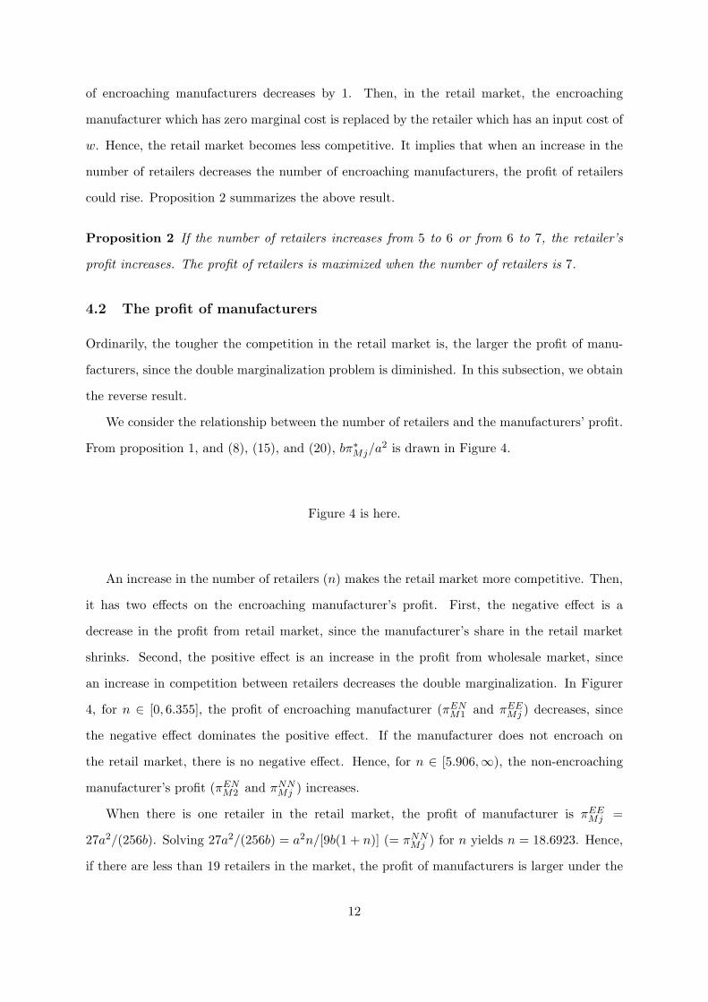
We consider the relationship between the number of retailers and the manufacturers’ profit.
From proposition 1, and (8), (15), and (20), bπ∗Mj/a2 is drawn in Figure 4.
Figure 4 is here.
An increase in the number of retailers (n) makes the retail market more competitive. Then,
it has two effects on the encroaching manufacturer’s profit. First, the negative effect is a
decrease in the profit from retail market, since the manufacturer’s share in the retail market
shrinks. Second, the positive effect is an increase in the profit from wholesale market, since
an increase in competition between retailers decreases the double marginalization. In Figurer
4, for n ∈ [0, 6.355], the profit of encroaching manufacturer (πENM1 and πEE
Mj ) decreases, since
the negative effect dominates the positive effect. If the manufacturer does not encroach on
the retail market, there is no negative effect. Hence, for n ∈ [5.906,∞), the non-encroaching
manufacturer’s profit (πENM2 and πNN
Mj ) increases.
When there is one retailer in the retail market, the profit of manufacturer is πEEMj =
27a2/(256b). Solving 27a2/(256b) = a2n/[9b(1 + n)] (= πNNMj ) for n yields n = 18.6923. Hence,
if there are less than 19 retailers in the market, the profit of manufacturers is larger under the
12
monopolistic retail market than the oligopolistic retail market. Proposition 3 summarizes the
above result.
Proposition 3 For n ≥ 6, an increase in the number of retailers (n) may decrease the en-
croaching manufacturer’s profit. The manufacturer’s profit is larger at n = 1 than at 2 < n < 18.
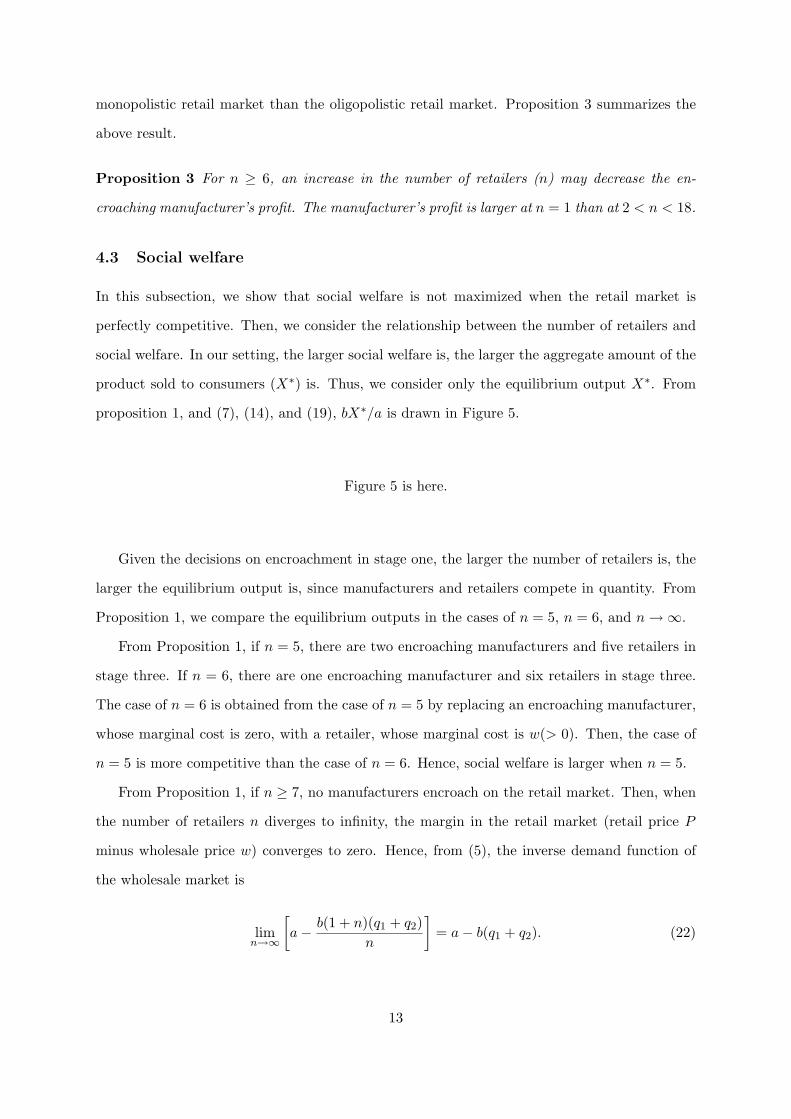
4.3 Social welfare
In this subsection, we show that social welfare is not maximized when the retail market is
perfectly competitive. Then, we consider the relationship between the number of retailers and
social welfare. In our setting, the larger social welfare is, the larger the aggregate amount of the
product sold to consumers (X∗) is. Thus, we consider only the equilibrium output X∗. From
proposition 1, and (7), (14), and (19), bX∗/a is drawn in Figure 5.
Figure 5 is here.
Given the decisions on encroachment in stage one, the larger the number of retailers is, the
larger the equilibrium output is, since manufacturers and retailers compete in quantity. From
Proposition 1, we compare the equilibrium outputs in the cases of n = 5, n = 6, and n →∞.
From Proposition 1, if n = 5, there are two encroaching manufacturers and five retailers in
stage three. If n = 6, there are one encroaching manufacturer and six retailers in stage three.
The case of n = 6 is obtained from the case of n = 5 by replacing an encroaching manufacturer,
whose marginal cost is zero, with a retailer, whose marginal cost is w(> 0). Then, the case of
n = 5 is more competitive than the case of n = 6. Hence, social welfare is larger when n = 5.
From Proposition 1, if n ≥ 7, no manufacturers encroach on the retail market. Then, when
the number of retailers n diverges to infinity, the margin in the retail market (retail price P
minus wholesale price w) converges to zero. Hence, from (5), the inverse demand function of
the wholesale market is
limn→∞
[a− b(1 + n)(q1 + q2)
n
]= a− b(q1 + q2). (22)
13

The above equation implies that the equilibrium retail price is equal to the equilibrium wholesale
price. Hence, when n → ∞, the equilibrium output X∗ converges to the total output in the
two-firm Cournot equilibrium with zero marginal cost. When there are no retailers, in the
retail market, there are two encroaching manufacturers. Hence, from (7) and (19), we obtain
limn→∞XNN = XEE |n=0 < XEE |n=1 < XEE |n=5. The inequalities are hold, because given the
decisions on encroachment, increases in the number of retailers lead to larger the equilibrium
output. Therefore, the monopolistic retail market gives a higher social welfare than the perfectly
competitive market. Proposition 4 summarizes the above result.
Proposition 4 Social welfare is maximized when n = 5. Social welfare in the case of n = 1 is
larger than that in the case as n →∞.
The existence of retailers causes a double marginalization problem. Thus, the non-existence
of retailers is usually desired. However, if the number of retailers is small enough to cause
manufacturers to encroach on the retail market, the existence of retailers is desirable for society.
Even if the retail market is monopoly, social welfare in the market is larger than the market
which includes no retailers. Therefore, we should not eliminate middleman.
5 Endogenous Number of Retailers: Divisionaliztion Problem
In the former section, we show that the number of retailers significantly affects on the equilibrium
outcomes. Actually, firms (especially retailers) can create their stores (e.g., supermarkets and
convenience stores). For example, to control the number of stores, retailers create division by
selling franchises without exclusive territories. Hence, it is important to consider the retail
market with endogenous number of retailers.
In our model, from Proposition 2, the retailer’s profit under 7 retailers is larger than under
monopolistic retail market. Then, retailers may have an incentive to create divisions. In this
section, we discuss the divisionalization problem in the retail market.
We assume that retailers cannot sell the product to consumer directly, and the divisions
created with no cost by retailers buy the product from manufacturers and sell it to consumers.
For simplicity, we assume that the retailer can only make a ‘take it or leave it’ offer for the
divisions. Thus, the profit of retailer is the sum of the divisions’ profit. That is, we consider
14

the former stage in which retailers simultaneously choose the number of divisions. Then, the
following stage is the same as former section.
We assume that divisions can be created with no cost. First, we consider that there is one
retailer in the market. Then, from the second equation in (8), the monopolistic retailer’s profit
is nπNNRi , where n is the number of divisions created by the retailer. Differentiating nπNN
Ri with
respect to n yields −4a2(n − 1)/[9b(1 + n)3] which is negative in n ≥ 7. From Proposition 2,
for n ≤ 6, the profit of division is smaller than n = 7. Hence, the monopolistic retailer creates
7 divisions in retail market. Then, from Proposition 1, manufacturers do not encroach on the
retail market. Corollary 1 summarizes the above argument.
Corollary 1 If a monopolistic retailer can create its division with no cost, it sells 7 franchises.
Then, manufacturers’ encroachment is deterred.
Next, we consider that the retail market is oligopoly. From Proposition 2, the aggregate
number of divisions created by retailers is not less than 7. Thus, manufacturers do not encroach
on the retail market. Let ni (resp. nk) be the number of the divisions created by retailer i
(resp. k), and n−i =∑
k 6=i nk. Then, from (8), the profit of retailer i is
πNNRi =
4a2ni
9b (1 + ni + n−i). (23)
The first-order condition for retailer i leads to the best response for the retailer i: ni = 1+n−i.
Hence, perfect competition is the equilibrium outcome, since all retailer want to set up one
more divisions than the aggregate number of divisions created by other retailers.
Corollary 2 When the retail market is oligopoly, perfect competition is the equilibrium outcome
in the divisionalization stage.
This result is the same as Corchon (1991). He does not consider vertical relationships and
show that divisionalization with no cost leads to perfect competition. Mizuno (forthcoming)
consider costly divisionalization in a vertical relationship, but does not consider manufacturer’s
encroachment. He shows that costly divisionalization does not lead to perfect competition.
In our model, manufacturers do not encroach on the retail market with the large number of
retailers. Thus, when divisionalization is costly, our result is the same as result in Mizuno
(forthcoming).
15

6 Oligopolistic Wholesale Market
In this section, we suppose the number of manufacturer m ≥ 2. The other settings are same
as in the section 2. Then, we show that if there are few retailers, all manufacturers encroach
on the retail market , but there are many retailers, they do not. This property is similar to
it in the former section. Hence, we find that our result is robust. At the end of this section,
we provide the number of retailers such that social welfare is maximized given the number of
manufacturers.
The profit of manufacturer j is
πMj =
a− b
m∑
j=1
dj +n∑
i=1
xi
dj + wqj . (24)
The profit of retailer i is
πRi =
a− b
m∑
j=1
dj +n∑
i=1
xi
− w
xi. (25)
This model can be solved in the similar way as in the section 3. We denote mE as the
number of encroaching manufacturers. Let mE be
mE =−2 + 2m− n +
√16 + 16m + 4m2 + 16n− 4mn + n2
6. (26)
If mE ≤ mE , the equilibrium profit of encroaching manufacturers in stage two is
πEM =
a2(1 + m + n + mmE −mE2)2
(1 + mE)2(−1−m + mE)2(1 + n + mE)2, (27)
where the superscript E denotes that the manufacturer encroaches on the retail market. The
profit of non-encroaching manufacturers in stage two is
πNM =
a2n
(1 + mE)(−1−m + mE)2(1 + n + mE), (28)
where the superscript N denotes that the manufacturer does not encroach on the retail market.
16

If mE > mE , the equilibrium profit of encroaching manufacturers in stage two is
πEM =
a2
Ω
1 + 2m + m2 + 2n + 2mn + m2n + n2 + 3mE + 6mmE
+3m2mE + 5nmE + 2m2nmE + 3n2mE + n3mE + 3mE2
+6mmE2 + 3m2mE
2 + 12nmE2 − 2mnmE
2 + m2nmE2
+6n2mE2 + mE
3 + 2mmE3 + m2mE
3 + 9nmE3
, (29)
where Ω = (1+n+mE)(1 + m + n + mn + 2mE + 2mmE − nmE + mnmE + mE2 + mmE
2)2.
The profit of non-encroaching manufacturers is
πNM =
a2n(1 + mE)(1 + n + 3mE)2
Ω. (30)
Figure 6 is here.
By numerical calculation, we obtain the ratio of the number of manufacturers encroaching
on the retail market in the equilibrium (See Figure 6). In Figure 6, s denotes the ratio of the
number of manufacturers, that is s = mE/m. If s = 1, all manufacturers encroach on the retail
market, and if s = 0, no manufacturers encroach. In the only 10 cases, some manufacturers
encroach on the retail market, and the others do not. There are multiple equilibria in which all
firms encroach and no firms encroach at some pair (m,n). Given the number of manufacturer
(m), all manufacturers encroach if there are few retailers, and no manufacturers encroach if
there are many retailers. Hence, we obtain the similar result in the former section.
Table 2 is here.
Table 2 shows the maximum number of retailers such that all manufacturers encroach nmax.
Since when all manufacturers encroach, social welfare increase with the number of retailers, the
social welfare is maximized at nmax. For example, when there are 10 manufacturers, nmax = 21
if the equilibrium must be unique, and nmax = 57 if the equilibria can be multiple. Then, social
17

welfare is maximized at n = 21 if the equilibrium must be unique, and at n = 57 if the equilibria
can be multiple. In Table 2, the larger the number of manufacturer is, the larger nmax is. Since
nmax progressively increases with the number of manufacturers under the multiple equilibria, if
the wholesale market is competitive, government should not regulate the retail market.
7 Conclusions
This paper analyzed supplier encroachment in successive oligopoly. We show that , social welfare
is larger when there are direct marketing manufacturers than when there are not. The following
constitute the main findings of this research. When there are six retailers, one manufacturer
sells only through the indirect sales channel, while the other sells only through the direct sales
channel. When the number of retailers exceeds 7, no manufacturers sells directly even if the
marginal cost of direct sales is zero. When an increase in the number of retailers decreases
the number of encroaching manufacturers, the profit of retailers could increases. When there
are five retailers, social welfare is maximized. When the retailers can create their divisions,
manufacturers’ encroachment is deterred. Even if there are m ≥ 2 manufacturers, the property
of the result in duopolistic wholesale market is held. We provide the number of retailers such
that social welfare is maximized given the number of manufacturer.
In our paper, we assume homogeneous products. However, some firms sell differentiated
products through direct and indirect sales channels. In the apparel industry, The Gap sells
clothes at company stores, that is, The Gap directly sells the clothes to consumer. Calvin Klein
sells clothes at department stores, that is, Calvin Klein indirectly sells the clothes.5 Therefore,
a study of relationship between product differentiation and direct marketing is also future
research.
5 For apparel industry, see Gertner and Stillman (2001).
18
Appendix
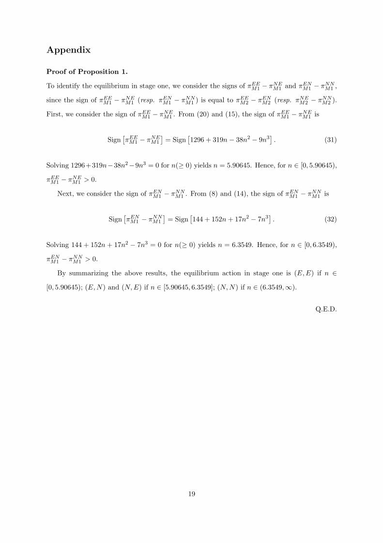
Proof of Proposition 1.
To identify the equilibrium in stage one, we consider the signs of πEEM1 − πNE
M1 and πENM1 − πNN
M1 ,
since the sign of πEEM1 − πNE
M1 (resp. πENM1 − πNN
M1 ) is equal to πEEM2 − πEN
M2 (resp. πNEM2 − πNN
M2 ).
First, we consider the sign of πEEM1 − πNE
M1 . From (20) and (15), the sign of πEEM1 − πNE
M1 is
Sign[πEE
M1 − πNEM1
]= Sign
[1296 + 319n− 38n2 − 9n3
]. (31)
Solving 1296+319n−38n2−9n3 = 0 for n(≥ 0) yields n = 5.90645. Hence, for n ∈ [0, 5.90645),
πEEM1 − πNE
M1 > 0.
Next, we consider the sign of πENM1 − πNN
M1 . From (8) and (14), the sign of πENM1 − πNN
M1 is
Sign[πEN
M1 − πNNM1
]= Sign
[144 + 152n + 17n2 − 7n3
]. (32)
Solving 144 + 152n + 17n2 − 7n3 = 0 for n(≥ 0) yields n = 6.3549. Hence, for n ∈ [0, 6.3549),
πENM1 − πNN
M1 > 0.
By summarizing the above results, the equilibrium action in stage one is (E, E) if n ∈[0, 5.90645); (E, N) and (N, E) if n ∈ [5.90645, 6.3549]; (N, N) if n ∈ (6.3549,∞).
Q.E.D.
19

References
[1] Arya, A., Mittendorf, B., and Sappington, D. E. M. (2007). “The bright side of supplier
encroachment”, Marketing Science, Vol. 26, No. 5, pp. 651–659.
[2] Baourakis, G., Kourgiantakis, M., and Migdalas, A. (2002). “The impact of e-commerce on
agro-food marketing. The case of agricultural cooperatives, firms and consumers in Crete”,
British Food Journal, Vol. 104, No. 8, pp. 508–590.
[3] Barkema, A., Drabenstott, M., and Welch, K. (1991). “The quiet revolution in the U.S. food
market”, Economic Review, Vol. 76, No. 3, pp. 25–41.
[4] Buehler, S. and Schmutzler, A. (2005). “Asymmetric vertical integration”, Advances in
Theoretical Economics, Vol. 5, No. 1, Art. 1.
Available at: http://www.bepress.com/bejte/advances/vol5/iss1/art1
[5] Chiang, W. K., Chhajed, D., and Hess, J. D. (2003). “Direct marketing, indirect profits: A
strategic analysis of dual-channel supply-chain design”, Management Science, Vol. 49, No.
1, pp. 1–20.
[6] Corchon, L. C. (1991). “Oligopolistic competition among groups”, Economics Letters, Vol.
36, No. 1, pp. 1–3.
[7] Gabszewicz, J. J. and Thisse, J. F. (1979). “Price competition, quality and income dispari-
ties”, Journal of Economic Theory, Vol. 20, No. 3, pp. 340–359.
[8] Gabszewicz, J. J. and Thisse, J. F. (1980) “Entry (and exit) in a differentiated industry”,
Journal of Economic Theory, Vol. 22, No. 2, pp. 327–338.
[9] Gertner, R. H. and Stillman, R. S. (2001) “Vertical integration and internet strategies in
the apparel industry”, Journal of Industrial Economics, Vol. 49, No. 4, pp. 417–440.
[10] Lahiri, Sajal and Ono, Yoshiyasu. (1988) “Helping minor firms reduces welfare”, Economic
Journal, Vol. 98, No. 393, pp. 1199–1202.
[11] Lin, P. (2006). “Strategic spin-offs of input divisions”, European Economic Review, Vol.
50, No. 4, pp. 977–993.
20
[12] Matsushima, N. (2006). “Industry profits and free entry in input markets”, Economics
Letters, Vol. 93, No. 3, pp. 329–336.
[13] Mizuno, T. “Divisionalization and horizontal mergers in a vertical relationship”, forthcom-
ing in Manchester School.
[14] Rogers, R. T. (2001). “ Structural change in U.S. food manufacturing, 1958-1997”,
Agribusiness, Vol. 17, No. 1, pp. 3–32.
[15] Salinger, M. A. (1988). “Vertical mergers and market foreclosure”, Quarterly Journal of
Economics, Vol. 103, No. 2, pp. 345–356.
[16] Salop, S. C. and Scheffman, D. T. (1983). “Raising rivals’ costs”, American Economic
Review Vol. 73, No. 2, pp. 267–271.
[17] Sexton, R. J. (2000). “Industrialization and consolidation in the U.S. food sector: impli-
cation for competition and welfare”, American Journal of Agricultural Economics, Vol. 82,
No. 5, pp. 1087–1104.
[18] Shaked, A. and Sutton, J. (1982). “Relaxing price competition through product differenti-
ation”, Review of Economic Studies, Vol. 49, No. 1, pp. 3–13.
[19] Shaked, A. and Sutton, J. (1983). “Natural oligopolies”, Econometrica, Vol. 51, No. 5, pp.
1469–1483.
[20] Sibley, D. and Weisman, D. (1998). “Raising rivals’ cost: The entry of an upstream mo-
nopolist into downstream markets”, Information Economics and Policy, Vol. 10, No. 4, pp.
451–470.
[21] United States Department of Agriculture. (2004). “2002 Census of agriculture. Market
value of agricultural products sold including direct and organic: 2002 and 1997.”
Available at: http://www.agcensus.usda.gov/Publications/2002/Volume 1, Chapter 1 US/
st99 1 002 002.pdf
[22] Wrigley, N. (2001). “The consolidation wave in U.S. food retailing: a European perspec-
tive”, Agribusiness, Vol. 17, No. 4, pp. 489–513.
21

[23] Ziss, S. (2005). “Horizontal merger and successive oligopoly”, Journal of Industry, Compe-
tition and Trade, Vol. 5, No. 2, pp. 99–114
22

Table 1.
Table 1: Encroachment decision
Manufacturer 2Encroachment (E) No-encroachment (N)
Manufacturer 1Encroachmet (E) πEE
M1 , πEEM2 πEN
M1 , πENM2
No-encroachment (N) πNEM1 , πNE
M2 πNNM1 , πNN
M2
23

Table 2.
The maximum number of retailers such that all manufacturers encroach (nmax).
The number of manufacturer 2 3 4 5 10 30 50 100 1000
nmax under unique equilibrium 5 4 7 11 21 61 101 201 2001
nmax under multiple equilibria 5 4 7 12 57 589 1,687 6,906 705,433
24

Figure 1.
Manufacturer Manufacturer
Wholesale
Market
Retailer Retailer
Retail
Market
q1 q2
w
x1 xn
d1 d2
Wholesale
Sales
Wholesale
Sales
Wholesale Price
Retail Sales Retail Sales
Direct Sales Direct Sales
25

Figure 2.
CostE
CostN
BenefitE
BenefitN
n
(N N)(E E) (N E)
(E N)
5.906 6.355
26

Figure 3.
2 4 6 8 10
0.002
0.004
0.006
0.008
b∗
Ri/ a
2
n
27
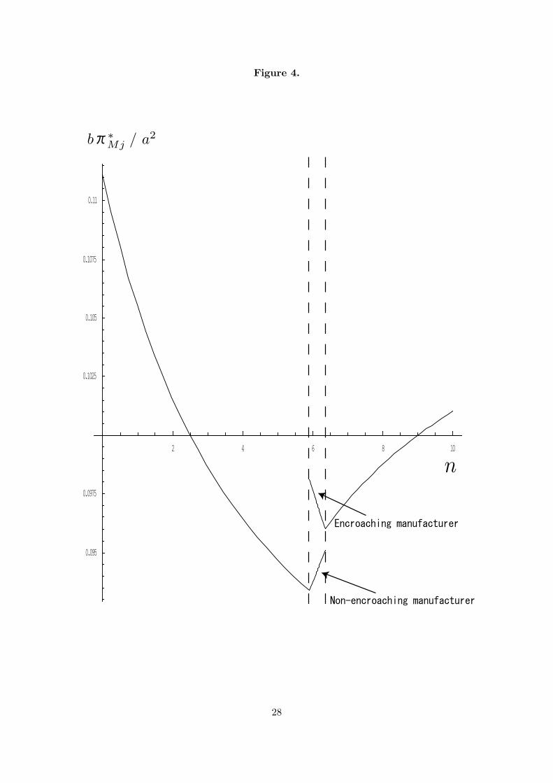
Figure 4.
2 4 6 8 10
0.095
0.0975
0.1025
0.105
0.1075
0.11
b∗
Mj / a2
n
28

Figure 5.
2 4 6 8 10
0.42
0.43
0.44
0.45
0.46
bX∗/ a
2
n
29

Figure 6.
(a)
0
20
40
0.5
0.75
0
20
40
0
0.25
1
m n
s
(b)
0
20
40
0
20
40
0
0.25
0.5
0.75
1
mn
s
30