diploma programme mathematics hl teaching notes hl... · diploma programme mathematics hl teaching...

b

DIPLOMA PROGRAMME

MATHEMATICS HL TEACHING NOTES

First examinations 2006

International Baccalaureate Organization

Buenos Aires Cardiff Geneva New York Singapore

562a

Diploma Programme

Mathematics HL teaching notes

International Baccalaureate Organization, Geneva, CH-1218, Switzerland

First published in April 2004 Updated February 2006

by the International Baccalaureate Organization

Peterson House, Malthouse Avenue, Cardiff Gate Cardiff, Wales GB CF23 8GL

UNITED KINGDOM

Tel: + 44 29 2054 7777 Fax: + 44 29 2054 7778 Web site: www.ibo.org

© International Baccalaureate Organization 2004

The IBO is grateful for permission to reproduce and/or translate any copyright material used in this publication. Acknowledgments are included, where appropriate, and, if notified, the IBO will be pleased to rectify any errors or omissions at the earliest opportunity.

IBO merchandise and publications in its official and working languages can be purchased through the online catalogue at www.ibo.org, found by selecting Publications from the shortcuts box. General ordering queries should be directed to the sales department in Cardiff.

Tel: +44 29 2054 7746 Fax: +44 29 2054 7779 E-mail: [email protected]

Printed in the United Kingdom by the International Baccalaureate Organization, Cardiff.

Mathematics HL teaching notes These notes provide additional guidance to teachers and include suggestions for using a graphic display calculator (GDC). A GDC is a useful tool for enhancing mathematical activity: teachers should encourage students to understand and interpret the results that a GDC provides. Further advice on the use of GDCs in the classroom can be accessed through discussion forums on the online curriculum centre (OCC).

Contents

Topic 1—Core: Algebra 1

Topic 2—Core: Functions and equations 2

Topic 3—Core: Circular functions and trigonometry 3

Topic 4—Core: Matrices 4

Topic 5—Core: Vectors 5

Topic 6—Core: Statistics and probability 6

Topic 7—Core: Calculus 8

Topic 8—Option: Statistics and probability 10

Topic 9—Option: Sets, relations and groups 13

Topic 10—Option: Series and differential equations 16

Topic 11—Option: Discrete mathematics 18

© International Baccalaureate Organization 2004 1

Topic 1—Core: Algebra

Teaching notes GDC suggestions

1.1 Use of infinite geometric series to express recurring decimals as rational numbers.

Link infinite geometric series with limits of convergence in 7.1.

Use of sequence mode can be useful.

Sequences can be generated and displayed in several ways.

Use recursive functions and options.

1.2 Exponents and logarithms are further developed in 2.7.

1.3 Link binomial theorem to binomial distribution in 6.10. For example, finding 6r⎛ ⎞⎜ ⎟⎝ ⎠

from 6nry C X= and then reading from the table.

Use recursive functions and options.

1.4 Links to a wide variety of topics, for example, complex numbers, matrices, differentiation, sums of series, divisibility.

Use recursion for checking and building hypotheses and disproving.

1.5 Conversion between forms using complex mode.

1.6 Calculations in complex mode.

1.7

1.8 Link conjugate roots of polynomials to 2.10.


Topic 2—Core: Functions and equations Teaching notes GDC suggestions

2.1 Examples: 2: , f x x x∈ (many-to-one); 2: , 0g x x x > (one-to-one).

If an inverse is to be found, a new one-to-one function may need to be defined. Link composite functions with the chain rule in 7.2.

Use of a GDC graph to visualize the range. Importance of the appropriate window. Note the limitations of a GDC in drawing inverses.

2.2 Basic graphing skills. More advanced graphing skills.

2.3 Link transformations of graphs with quadratic functions 2.5, exponential functions 2.7 and 2.8, and circular functions 3.4.

Use of a GDC to investigate these transformations. Use of a regression tool to find the curve of best fit will enhance portfolio modelling activities. Use of lists to generate families of curves.

2.4

2.5

2.6 A program on the GDC for the quadratic formula can be helpful. Solutions of more complicated equations may be found with the “solve” features of GDCs.

2.7 Link exponential functions with inverses in 2.3 and with exponents in 1.2. Displaying the graph of a function and its inverse can be helpful, but the reflective property is not apparent unless axes are scaled equally.

2.8

2.9

2.10 Link the solution of polynomial equations to conjugate roots in 1.8. Use of GDCs to find zeros.


Topic 3—Core: Circular functions and trigonometry


3.1

3.2

3.3 Demonstration of double angle formulae and other trigonometric identities.

3.4 Transformation of all trigonometric graphs and their inverses.

3.5 Link to 2.3. Graphical solution of trigonometric equations.

Use “Test” function in solver mode.

3.6 Cosine rule may be proved using scalar product.


Topic 4—Core: Matrices


4.1

4.2 Entry of matrices into a GDC, and algebraic manipulation using a GDC.

4.3 Finding the determinant and the inverse of a 3 3× matrix using a GDC.

4.4 Augmented matrix definition. Solution of 3 equations in 3 unknowns using matrices.

Use “rref ” to test for types of solutions.


Topic 5—Core: Vectors


5.1 Vector sums and differences can be represented by the diagonals of a parallelogram.

Multiplication by a scalar can be illustrated by enlarging the vector parallelogram.

Applications to simple geometric figures, for example, ABCD is a

quadrilateral and AB CD ABCD→ →

= − ⇒ is a parallelogram.

Use column matrices and list mode (with vertical alignment) and list operations to manipulate vectors.

Use different methods of manipulating vectors.

5.2 Properties of the scalar product

⋅ = ⋅v w w v ;

( )⋅ + = ⋅ + ⋅u v w u v u w ;

( ) ( )k k⋅ = ⋅v w v w ;

2⋅ =v v v .

This is an opportunity for allowing students to develop programs for calculations.

5.3

5.4

5.5 Use row reduction form to solve problems.

5.6

5.7


Topic 6—Core: Statistics and probability


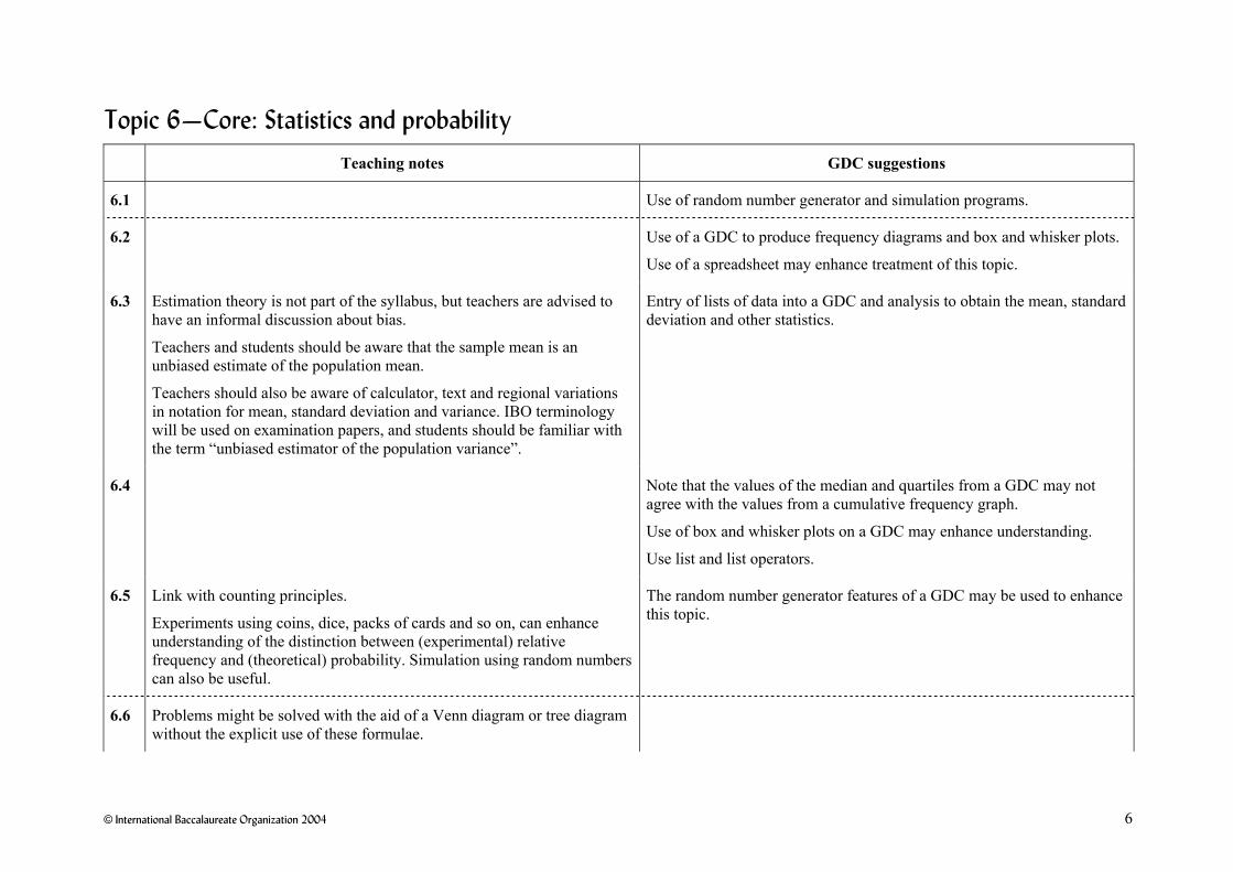
6.1 Use of random number generator and simulation programs.

6.2 Use of a GDC to produce frequency diagrams and box and whisker plots.

Use of a spreadsheet may enhance treatment of this topic.

6.3 Estimation theory is not part of the syllabus, but teachers are advised to have an informal discussion about bias.

Teachers and students should be aware that the sample mean is an unbiased estimate of the population mean.

Teachers should also be aware of calculator, text and regional variations in notation for mean, standard deviation and variance. IBO terminology will be used on examination papers, and students should be familiar with the term “unbiased estimator of the population variance”.

Entry of lists of data into a GDC and analysis to obtain the mean, standard deviation and other statistics.

6.4 Note that the values of the median and quartiles from a GDC may not agree with the values from a cumulative frequency graph.

Use of box and whisker plots on a GDC may enhance understanding.

Use list and list operators.

6.5 Link with counting principles.

Experiments using coins, dice, packs of cards and so on, can enhance understanding of the distinction between (experimental) relative frequency and (theoretical) probability. Simulation using random numbers can also be useful.

The random number generator features of a GDC may be used to enhance this topic.

6.6 Problems might be solved with the aid of a Venn diagram or tree diagram without the explicit use of these formulae.


Topic 6—Core: Statistics and probability (continued)


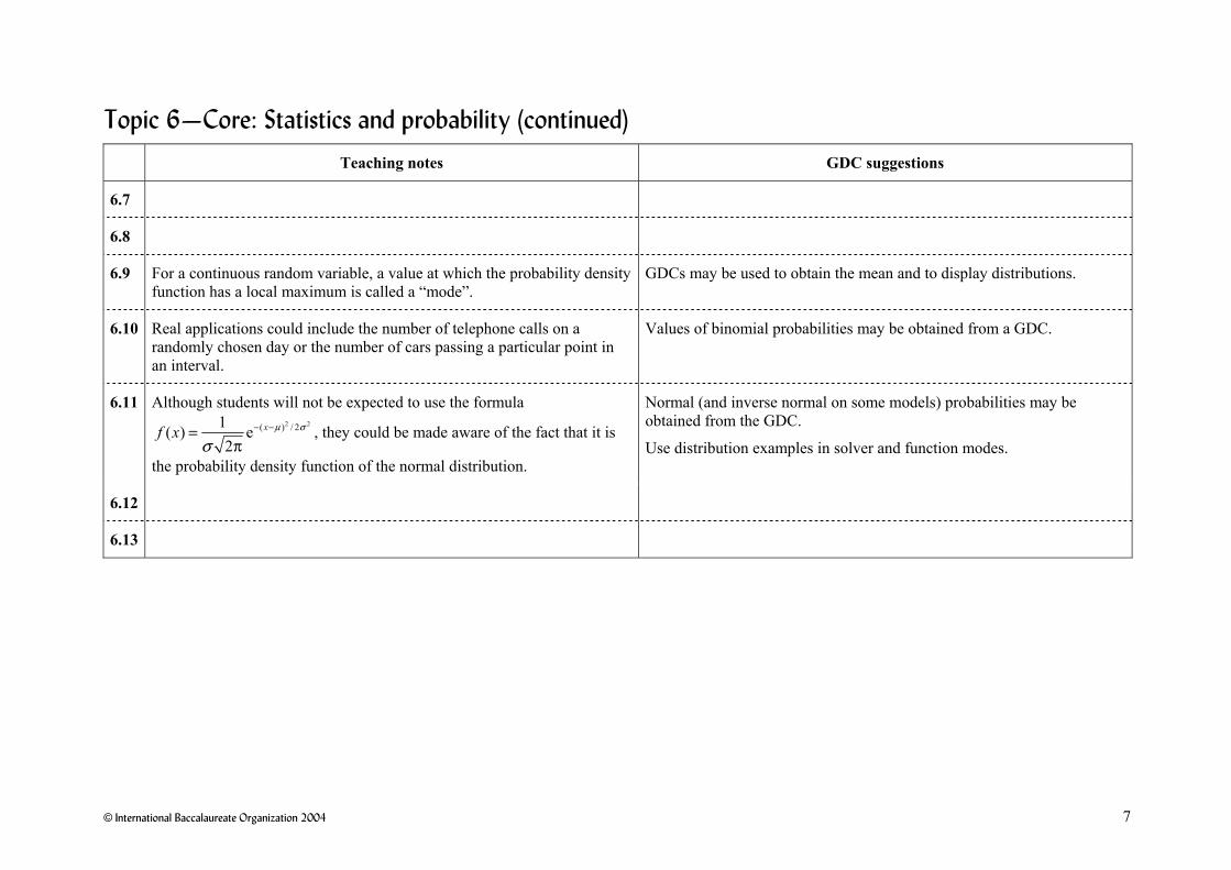
6.7

6.8

6.9 For a continuous random variable, a value at which the probability density function has a local maximum is called a “mode”.

GDCs may be used to obtain the mean and to display distributions.

6.10 Real applications could include the number of telephone calls on a randomly chosen day or the number of cars passing a particular point in an interval.

Values of binomial probabilities may be obtained from a GDC.

6.11 Although students will not be expected to use the formula 2 2( ) / 21( ) e

2xf x µ σ

σ− −=

π, they could be made aware of the fact that it is

the probability density function of the normal distribution.

Normal (and inverse normal on some models) probabilities may be obtained from the GDC.

Use distribution examples in solver and function modes.

6.12

6.13


Topic 7—Core: Calculus


7.1 Link convergence with infinite geometric series in 1.1.

Link use of definition of derivative with binomial theorem in 1.3.

Sketch graph of ( )f x′ from graph of ( )y f x= and vice versa.

Investigation of limits numerically.

Graphical investigation and justification of derivatives.

Finding gradient functions and equations of tangents.

Functions other than polynomials, for example, derivative of ex , sin x and cos .x

Note that the graph and equation of the tangent, the tangent line (and normal or normal line on some models) is available at the touch of a button.

7.2 Link chain rule with composite function in 2.1.

Link chain rule with implicit differentiation in 7.8 and integration by parts in 7.9.

A GDC may be used to verify results.

7.3 Link with graphing functions in 2.2. Finding maximum and minimum points.

A GDC may be used to display f, f ′ and .f ″

Use f ′ and f ″ in graph mode.

7.4 Students should be made aware of the fundamental theorem of calculus,

( ) ( )d ( ) ( )x

aF x f t t F x f x′= ⇒ =∫ , and discuss its graphical interpretation.

Slope field diagrams could be used to enhance understanding of families of curves.


Topic 7—Core: Calculus (continued)


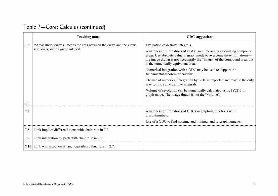
7.5 “Areas under curves” means the area between the curve and the x-axis (or y-axis) over a given interval.

Evaluation of definite integrals.

Awareness of limitations of a GDC in numerically calculating compound areas. Use absolute value in graph mode to overcome these limitations—the image drawn is not necessarily the “image” of the compound area, but is the numerically equivalent area.

Numerical integration with a GDC may be used to support the fundamental theorem of calculus.

The use of numerical integration by GDC is expected and may be the only way to find some definite integrals.

Volume of revolution can be numerically calculated using [Y2]^2 in graph mode. The image drawn is not the “volume”.

7.6

7.7 Awareness of limitations of GDCs in graphing functions with discontinuities.

Use of a GDC to find maxima and minima, and to graph tangents.

7.8 Link implicit differentiations with chain rule in 7.2.

7.9 Link integration by parts with chain rule in 7.2.

7.10 Link with exponential and logarithmic functions in 2.7.


Topic 8—Option: Statistics and probability


8.1

8.2 The cumulative distribution function (cdf) of a random variable X is the probability that X takes a value less than or equal to x, that is

( ) P( )F x X x= ≤ .

The probability mass function is the probability function of a discrete random variable X such that P( )xp X x= = . Example: if

( )~ B ,X n p , ( )1 n xxx

np p p

x−⎛ ⎞

= −⎜ ⎟⎝ ⎠

.

For a discrete distribution, the cdf ( ) yy x

F x p≤

=∑ .

For a continuous distribution ( ) ( )dx

F x f t t−∞

= ∫ where ( )f x is the

probability density function (pdf) of X.

The Bernoulli distribution is the binomial distribution with 1n = .

The negative binomial distribution is sometimes known as Pascal’s distribution. This is the probability distribution for the number of Bernoulli trials required for r successes. If 1r = , the negative binomial distribution reduces to the geometric distribution.


Topic 8—Option: Statistics and probability (continued)


8.3 It is expected that students will have an appreciation of the normal approximation to the binomial as an example of the central limit theorem. On examination papers the continuity correction will not be required.

For large samples from a population where P, the population proportion, is not too close to 0 or 1, the distribution of the sample proportion is well approximated by the normal distribution. A common but rather conservative rule for the application of this approximation is 10nP ≥ and

(1 ) 10n P− ≥ .

8.4 Confidence intervals calculated with the normal distribution and with the t-distribution. The conditions under which these distributions are used in the calculation of confidence intervals for the mean. With the advent of modern calculators and statistical software, the t-distribution can be used in the case where σ is unknown and the parent population is normal for both large and small samples.

Large sample confidence interval.

In some texts and on some calculators the unbiased estimate of the population variance uses alternative notation, for example,

2 2 2 21ˆ , , , .n x xsσ σ σ−


Topic 8—Option: Statistics and probability (continued)


8.5 The z-test and the t-test. The conditions under which these tests apply.

With the advent of statistical software packages and advanced calculator functions, the restriction on the use of t-distribution to small samples is no longer necessary. The t-test can be used in the case where σ is unknown and the parent population is normal for both large and small samples.

Large sample test.

The p-value is the observed significance level. It is the probability of observing a test statistic equal to or more extreme than the observed one, assuming that 0H is true.

8.6 Degrees of freedom is number of classes – number of restrictions. For example, in a Poisson distribution if m is given, then the only restriction would be that the sum of the observed frequencies is the sum of the expected frequencies. Hence 1nν = − .

However, in the case of a Poisson distribution where m needs to be estimated from the sample, there would then be two restrictions and hence

2nν = − .


Topic 9—Option: Sets, relations and groups


9.1 Include the term “proper subset” and the distinction between A B⊂ and .A B⊆ Note that the empty set ∅ is not a proper subset.

Examples of set operations on finite and infinite sets will assist understanding.

Set difference: \ .A B A B′= ∩

Symmetric difference: ( \ ) ( \ ).A B A B B A∆ = ∪

Direct proof of the equality of sets using these laws. Example: ( \ ) ( \ ) ( ) ( ) .A B B A A B A B ′∪ = ∪ ∩ ∩

Illustration by Venn diagram is not a proof.

De Morgan’s laws are ( )A B A B′ ′ ′∪ = ∩ and ( ) .A B A B′ ′ ′∩ = ∪

9.2 Include examples and visual representations of relations.

For example: arrow diagrams and Cartesian graphs are standard visual representations of relations that aid understanding.

9.3 The term “codomain” is needed for this topic. An injection is also known as a one-to-one function, a surjection as an onto function and a bijection as a one-to-one correspondence.

Prove a function is an injection from the definition ( ) ( )f x f y x y= ⇒ = or by proving ( ) 0f x′ > or ( ) 0f x′ < over the given domain, if it is differentiable.

Proving a function is not a surjection is a good illustration of proof by counter-example.


Topic 9—Option: Sets, relations and groups (continued)


9.4 Examples of binary operations that are closed and those that are not closed will assist understanding.

9.5

9.6 The left-cancellation law is that ;a b a c b c∗ = ∗ ⇒ = , , .a b c G∈

The right-cancellation law is that ;b a c a b c∗ = ∗ ⇒ = , , .a b c G∈

9.7 Abelian groups are also known as commutative groups.

To prove ( , )G ∗ is an Abelian group it is necessary to prove the four properties of a group plus the commutative property. If G is a finite group, it is sufficient to refer to the symmetries of the operation table.

9.8 Another common representation for the permutation 1 3,→ 2 1,→ 3 2→ is the cycle notation (13 2).

9.9 Every finite group has the Latin square property but not conversely.

Arguments based on tables cannot be used to prove that a set with an infinite number of elements is a group.

9.10 Generators for cyclic groups.


Topic 9—Option: Sets, relations and groups (continued)


9.11 A proper subgroup of G is a subgroup of G that is not G itself.

Lagrange’s theorem is: Let H be a subgroup of the finite group G. Then the order of H divides the order of G. This does not imply that if the order of a finite group G has a factor n then there must exist a subgroup of G of order n.

The proof of Lagrange’s theorem provides a good illustration of a partition of a set (but the proof will not be examined).

9.12 An example of isomorphic groups are positive real numbers under multiplication and real numbers under addition.

Isomorphism can be demonstrated using the group tables for the symmetries of an equilateral triangle and the permutations on three elements of a set.

It may be possible to set up an isomorphism between two groups in more than one way.

In any isomorphism between two groups, the corresponding elements must be of the same order.

To show two finite groups are isomorphic, it is sufficient to list the bijection between the elements of the groups, and show that the two tables have the same structure.


Topic 10—Option: Series and differential equations


10.1 This improper integral is intended to meet the needs of the integral test.

These lower and upper sums are often referred to as the lower Riemann sum and the upper Riemann sum.

10.2 Convergence of an infinite series should be introduced through the convergence of the sequence of partial sums.

Examples (telescoping series): 1

1 ,( 1)n n n

∞

= +∑ 1

2 1 .( 1)( 2)n

nn n n

∞

=

++ +∑

The limit comparison test states that if na∑ and nb∑ are series of

positive terms with lim ,n

nn

a Lb→∞

= and L is a number greater than 0, then the

series either converge together or diverge together.

Example (integral estimate): 2 21 1

1 1 ,n

nk k

Rk k

∞

= =

= +∑ ∑ where 2

10 d .n nR x

x∞

< < ∫

10.3 It is useful to explain that

1

1n

∞

∑ is divergent, but that 1

1( 1)n

n

∞

−∑ is

convergent.

The series 1

21

( 1)n

n n

+∞

=

−∑ converges absolutely whereas the series 1

1

( 1)n

n n

+∞

=

−∑

converges conditionally.

10.4 Including power series in ( )x a− where 0.a ≠


Topic 10—Option: Series and differential equations (continued)


10.5 The Lagrange error term is

( 1)1( )( ) ( )

( 1)!

nn

nf cR x x an

++= −

+, for c between a

and x.

The integral form of the error term is ( 1) ( )( ) ( ) d .

!

nx nn a

f tR x x t tn

+

= −∫

10.6 Slope fields are sometimes called tangent fields or direction fields. This graphical approach to solution curves is well-suited to a GDC or a computer.

The substitution y vx= transforms the homogeneous differential equation into a variables separable differential equation.

The integrating factor for the differential equation ( ) ( )y p x y q x′ + = is ( )d

e .p x x∫


Topic 11—Option: Discrete mathematics


11.1 The division algorithm states that for any non-negative integer a and any positive integer b, there exist unique integers q and r with 0 ,r b≤ < such that .a bq r= +

The integer d is the greatest common divisor of a and b, denoted gcd( , )a b if (i) d a and d b , and (ii) if c a and c b , then .c d≤

Students should be able to prove results such as: gcd( , ) gcd( , );a b a a b= − gcd( , ) gcd( , )a b b r= where ;r a bq= − if gcd( , )a b d= then

gcd , 1.a bd d

⎛ ⎞ =⎜ ⎟⎝ ⎠

The integer m is the least common multiple of a and b, denoted lcm( , )a b if (i) a m and ,b m and (ii) if a n and ,b n then .n m≥

The fundamental theorem of arithmetic states that any positive integer greater than 1 has a unique prime factorization. From the fundamental theorem of arithmetic it follows that any positive integer 1n > has a unique prime-power decomposition, 1 2

1 2 ... ,kee ekn p p p= where the ie are

positive integers and the ip are distinct primes. Prime-power decomposition provides an alternate approach to calculating the gcd and lcm of two integers. The fundamental theorem of arithmetic can be used to prove such results as 2 is irrational and that there are infinitely many prime numbers.

11.2 Examples: express 5(1234) in the decimal system; express 732 in base 2.


Topic 11—Option: Discrete mathematics (continued)


11.3 The linear diophantine equation ax by c+ = has a solution if and only if (gcd( , )) .a b c One solution can be found by reversing the Euclidean algorithm and thereby the general solution. Often a better way to solve the equation is to solve the corresponding linear congruence (mod ).ax c b≡

11.4 By definition a is congruent to b modulo m, denoted (mod ),a b m≡ if ( ).m a b− It follows that if (mod )a b m≡ then there is an integer k such

that a b km= + and that a and b leave the same remainder on division by m. This means that every integer is congruent to a number in the set { }0,1,2,..., 1 .m − This set is known as the set of least residues.

The following properties of modular arithmetic:

if (mod )a b m≡ and (mod )c d m≡ then ( ) ( )(mod );a c b d m+ ≡ + ( ) ( )(mod );a c b d m− ≡ − (mod );ac bd m≡ (mod );n na b m≡

if (mod )ac bc m≡ and gcd( , ) 1,c m = then (mod )a b m≡ .

The linear congruence (mod )ax b m≡ has a solution if and only if (gcd( , )) | .a m b Furthermore, if a solution exists, there are gcd( , )a m non-congruent solutions modulo m.

The Chinese remainder theorem states that the system of congruences (mod ),i ix a m≡ 1,2,...,i k= where gcd( , ) 1i jm m = if ,i j≠ has a unique

solution modulo 1 2... .km m m

Example: find x such that 1(mod 2),x ≡ 2 3(mod7),x ≡ 8(mod15).x ≡




11.5 Fermat’s little theorem is often stated in the form: If p is prime and a is relatively prime to p, then ( )1 1 mod .pa p− ≡ Example: find the remainder when 193204 is divided by 97.

11.6 Isomorphism between simple graphs can be illustrated using a bijection between the vertex sets that preserves adjacency of edges, and using the adjacency matrices of the graphs.

11.7

11.8 Let G have vertex set { }1 2, ,..., pv v v and adjacency matrix GA . Then the

entry in the ith row and jth column of nGA is the number of different walks

of length n beginning at iv and ending at .jv This result can be proved by induction.

The weights of the edges in a complete graph may be given by its cost adjacency matrix .GC

11.9 Kruskal’s and Prim’s algorithms determine a minimum spanning tree in a connected weighted graph.

Dijkstra’s algorithm determines a shortest path between two specified vertices in a connected weighted graph.

Note that these algorithms are “greedy” since at each step they seek as much improvement as possible within the constraints of the problem.




11.10 The Chinese postman problem is to find the closed walk of minimum weight in a weighted connected graph, which includes each edge at least once. If the graph has no odd vertices, the solution is any Eulerian circuit. To find the solution when there are just two vertices of odd degree, find the shortest route between these vertices by Dijkstra’s algorithm or inspection. The postman must then walk along this shortest route twice and each of the other edges once. This is sometimes referred to as the “route inspection problem”.

Checking all Hamiltonian cycles finds the solution to the travelling salesman problem (TSP) but this method is inefficient.

A lower bound for the TSP may be found by removing one vertex from the graph together with all the edges leading into it. The minimum spanning tree is then found for this reduced graph. The vertex that has been removed is then reconnected to the minimum spanning tree via the two edges of least weight. The total weight of the minimum spanning tree and these two edges provides a lower bound for the TSP. This can be repeated for each of the vertices in the original graph and the highest of these taken as the “best” lower bound.

An upper bound can be found by doubling the weight of a minimum spanning tree.

diploma programme mathematics hl teaching notes hl... · diploma programme mathematics hl teaching...

Documents