dimension reduction of chemical process simulation data

Dimension Reduction of Chemical ProcessSimulation Data

Gabor Janiga1 and Klaus Truemper2

1Laboratory of Fluid Dynamics and Technical Flows,University of Magdeburg “Otto von Guericke”,

39106 Magdeburg, Germany2Department of Computer Science,

University of Texas at Dallas,Richardson, TX 75083, U.S.A.

Corresponding author:G. [email protected]

Abstract. In the analysis of combustion processes, simulation is a cost-efficient tool that complements experimental testing. The simulationmodels must be precise if subtle differences are to be detected. Onthe other hand, computational evaluation of precise models typicallyrequires substantial effort. To escape the computational bottleneck, re-duced chemical schemes, for example, ILDM-based methods or the flameletapproach, have been developed that result in substantially reduced com-putational effort and memory requirements.

This paper proposes an additional analysis tool based on the MachineLearning concepts of Subgroup Discovery and Lazy Learning. Its goal iscompact representation of chemical processes using few variables. Ef-ficacy is demonstrated for simulation data of a laminar methane/aircombustion process described by 29 chemical species, 3 thermodynamicproperties (pressure, temperature, enthalpy), and 2 velocity components.From these data, the reduction method derives a reduced set of 3 vari-ables from which the other 31 variables are estimated with good accuracy.

Key words: dimension reduction, subgroup discovery, lazy learner, modelingcombustion

1 Introduction

Virtually all transportation systems and the majority of electric power plantsrely directly or indirectly on the combustion of fossil fuels. Numerical simulationhas become increasingly important for improving the efficiency of these com-bustion processes. Indeed, simulation constitutes a cost-efficient complement ofexperimental testing of design prototypes.

2 Dimension Reduction of Simulation Data

A key demand is that simulation be precise since otherwise subtle differencesof complex processes escape detection. For example, the analysis of quantita-tive problems like predictions of intermediate radicals, pollutant emissions, orignition/extinction limits requires complete chemical models [6]. Until recently,most models have been 1- or 2-dimensional due to the huge computational effortrequired for 3-dimensional models; see [11, 9] for the computational effort carriedout for some 3-dimensional models.

Reduced chemical schemes, for example, ILDM-based methods or the flameletapproach [17], lead to a considerable speed-up of the computations when com-pared with a complete reaction mechanism, with small loss of accuracy. Theydrastically reduce required computational memory as well. These chemical schemesare based on an analysis of chemical pathways that identifies the most importantones. The other reactions are then modeled using the main selected variables.

This paper proposes an additional analysis tool called REDSUB that is basedon Machine Learning methods, specifically Subgroup Discovery [12, 19] and theconcept of Lazy Learner [15]. It analyses simulation data of chemical processesusing a complete reaction scheme and searches for a compact representation thatuses fewer variables while keeping errors within specified limits.

To demonstrate efficacy, a laminar methane/air burner is considered thatoccurs in many practical applications. The numerical simulation evaluates a2-dimensional model using detailed chemistry [10]. For each grid point, the sim-ulation produces values for 29 chemical species, 3 thermodynamic properties(pressure, temperature, enthalpy), and 2 velocity components. Given this infor-mation, REDSUB selects 3 variables from which the values of the remaining 31variables are estimated with good accuracy.

We begin with a general definition of the reduction problem. Let X be a finitecollection of vectors in Rn, the n-dimensional real space. In the present setting,X contains the results of a simulation model for some process. For efficient useof X, for example, for optimization purposes, we want to select a small subset Jof {1, 2, . . . , n} and construct a black box so that the following holds. For anyvector of x ∈ X, the black box accepts as input the xj , j ∈ J , and outputs valuesthat are close estimates of the xj , j /∈ J .

For a simplified treatment of numerical accuracy and tolerances, we translate,scale, and round values of vectors x ∈ X so that the entries become uniformlycomparable in magnitude. Thus, we select translation constants, scaling, androunding so that all variables have integer values ranging from 0 to 106, withboth bounds achieved on X. From now on we assume that the vectors of Xthemselves are of this form.

In the situations of interest here, we are given some additional information.Specifically, with each vector of x ∈ X an associated m-dimensional vector yof Rm and the value of a real function F (x) are supplied. For given input xj ,j ∈ J , the above black box must also output a close estimate of the functionvalue F (x). On the other hand, the black box need not supply estimates of thevalues of the vector y.

Dimension Reduction of Simulation Data 3

The reader may wonder why we introduce the function value F (x), since itcould be declared to be an additional entry in the vectors of X. In a momentwe introduce an assumption about the function F (·), and for that reason it isconvenient to treat its values separately.

As a final condition that is part of the problem definition, the index setJ selected in the reduction process must be a subset of a specified nonemptyset I ⊆ {1, 2, . . . , n} and must contain a possibly empty subset M ⊆ I. Forexample, the xj , j ∈ I, may represent values that are easily measured in thelaboratory and thus support a simplified partial verification of the full modelvia the reduced model. The subset M contains the indices of variables that werequire in the reduced model for any number of reasons.

In the example combustion process discussed in Section 3, each vector x ∈ Xcontains n = 33 values for various chemical components, temperature, pressure,and two velocities. The function F (x) is the enthalpy. The associated vectory ∈ Rm has m = 2 and defines the point in the plane to which the values of xand F (x) apply. Problem of that size are easily handled by REDSUB. Indeed,in principle the method can handle cases where the vectors x of X have up toseveral hundred entries. The size of m is irrelevant.

Once REDSUB has identified the index set J , the Lazy Learner of REDSUBcan use J and the set X to estimate for any vector where just the values xj ,j ∈ J are given, the values for all xj , j /∈ J , and F (x). This feature allowsapplication of the results in settings similar to that producing X.

We introduce two assumptions concerning the vectors y and the functionF (x). They are motivated by the applications considered here. The first as-sumption says that the vectors y constitute a particular sampling of a compactconvex subspace of Rm. The second one demands that F (·) is close to being aone-to-one function on the data set X.

Assumption 1 Collectively, the vectors y associated with the vectors x ∈ Xconstitute a grid of some compact convex subset of Rm.

Assumption 2 F (·) is close to being a one-to-one function, in the sense thatthe number of distinct function values F (x), x ∈ X, is close to the number ofvectors in X.

We motivate the assumptions by the combustion processes we have in mind.There, the vectors y are the coordinate values of the 1-, 2-, or 3-dimensionalsimulation. Since the simulation generates the points of a grid, Assumption 1 istrivially satisfied. Assumption 2 demands that the function distinguishes betweenalmost all points x ∈ X. In the example application discussed later, the functionis the enthalpy of the process and turns out to satisfy Assumption 2.

The paper proceeds as follows. The next section, 2, describes Algorithm RED-SUB. Section 3 covers application of the method to a methane combustion pro-cess. Section 4 has details of the subgroup discovery method used in REDSUB.Section 5 summarizes the results.


2 Algorithm REDSUB

In a traditional approach for the problem at hand, we could (1) estimate thefunction values with ridge regression [7, 8]; (2) derive the index set J via theestimating coefficients of the ridge regression equations of (1) and covarianceconsiderations; and (3) use ridge regression once more to compute estimatingequations that estimate values for the variables j /∈ J , and F (x) from those forthe variables xj , j ∈ J . The approach typically requires that the user specifiesnonlinear transformations of the variables for the regression steps (1) and (3).Here, we propose a new approach that is based on two Machine Learning con-cepts and does not require user-specified nonlinear transformations. Specifically,we use Subgroup Discovery [12, 19] to select interesting indices j from the set I;from these indices, the set J is defined. Then we use the concept of Lazy Learnerto predict values for the xj , j /∈ J , and F (x).

2.1 Subgroup Discovery

The Subgroup Discovery method, called SUBARP, constructs polyhedra thatrepresent important partial characterizations of level sets {x ∈ X | F (x) ≥ c} ofF (·) for various values c. SUBARP has been constructed from the classificationmethod Lsquare [2–5] and the extension of [18], using the general constructionscheme of [14] for deriving subgroup discovery methods from rule-based classifi-cation methods. Details are included in Section 4.

The key arguments for use of the polyhedra are as follows.If a variable occurs in the specification of a polyhedron, then control of the

value of that variable is important if function values are to be in a certain levelset. This is a direct consequence of the fact that Subgroup Discovery constructedthe polyhedron. Accordingly, the frequency qj with which a variable xj occursin the definition of the various polyhedra is a measure of the importance thevariable generally has for inducing function values F (·).

The frequency qj is computed as follows. Define the length of an inequalityto be the number of its nonzero coefficients. For a given polyhedron, the contri-bution to qj is 0 if xj does not occur in any inequality of the polyhedron, andotherwise is 1/k where k is the length of the shortest inequality containing xj .

For a simplified discussion, momentarily assume that indices j of high fre-quencies qj constitute the set J . We know that the variables xj , j ∈ J , areessential for determining the level sets of F (·). By Assumption 2, F (·) is closeto being a one-to-one function; thus, function values F (x) or, equivalently, levelsets may be used to estimate x vectors. Since variables xj , j ∈ J , are importantfor determining level sets of F (·), we know that such xj are also important fordetermining entire x vectors, in particular, for estimating values of the variablesxj , j /∈ J .

The actual construction of the set J is a bit more involved and involves iter-ative steps carried out by REDSUB. Details are discussed after the descriptionof the Lazy Learner. Here we mention only that REDSUB splits the input dataset X, which from now on we call a learning set, 50/50 into a training set S and


testing set T . The split is done in such a way that the y vectors correspondingto the vectors of S constitute a coarser subgrid of the original grid. SUBARPutilizes both sets S and T , while the Lazy Learner only uses S.

2.2 Lazy Learner

A Lazy Learner is a method that, well, never learns anything. Instead, it di-rectly derives from a given training set an estimate for the case at hand andthen discards any insight that could be gained from those computations [15]. Inthe present situation, given index set J and training set S, the Lazy Learnerestimates for a given vector x the entries xj , j /∈ J , and F (x) from the xj , j ∈ J .This section describes that estimation process, which is a particular LocallyWeighted Learning algorithm; see [1] for an excellent survey.

For the given vector x, let v be the subvector of x indexed by J , and definek = |J |. We first find a vector x1 ∈ S whose subvector z1 indexed by J is closestto v according the infinity norm, which defines the distance between any twovectors g and h to be maxj{|gj−hj |)}. We use that distance measure throughoutunless distance is explicitly specified to be Euclidean.

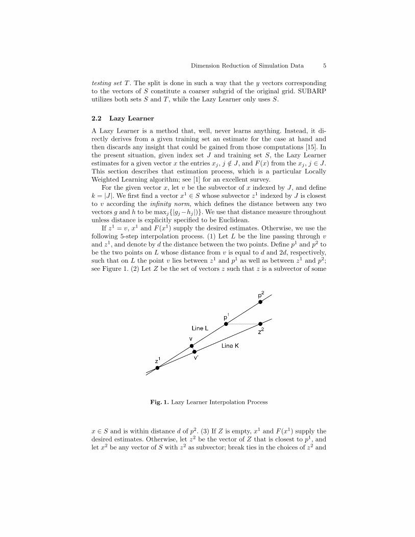
If z1 = v, x1 and F (x1) supply the desired estimates. Otherwise, we use thefollowing 5-step interpolation process. (1) Let L be the line passing through vand z1, and denote by d the distance between the two points. Define p1 and p2 tobe the two points on L whose distance from v is equal to d and 2d, respectively,such that on L the point v lies between z1 and p1 as well as between z1 and p2;see Figure 1. (2) Let Z be the set of vectors z such that z is a subvector of some

Fig. 1. Lazy Learner Interpolation Process

x ∈ S and is within distance d of p2. (3) If Z is empty, x1 and F (x1) supply thedesired estimates. Otherwise, let z2 be the vector of Z that is closest to p1, andlet x2 be any vector of S with z2 as subvector; break ties in the choices of z2 and


x2 arbitrarily. (4) Project v onto the line K passing through z1 and z2, gettinga point v′. The projection uses Euclidean distance. (5) If the point v′ lies on theline segment of K defined by z1 and z2 and thus is a convex combination of z1

and z2, say v′ = λz1+(1−λ)z2 for some λ ∈ [0, 1], then the vector λx1+(1−λ)x2

and λF (x1)+(1−λ)F (x2) provide the desired estimates. Otherwise, use x1 andF (x1) to obtain the estimates.

The above choices of distance measure and interpolation were derived viaexperimentation. Indeed, the infinity norm emphasizes maximum deviations,and with that measure, the interpolation seemingly is effective in producingestimates of uniform accuracy for the entire range of variables and the functionF (x).

The estimation errors for any vector x of the testing set T is the distancebetween the vector [x, F (X)] and the corresponding vector of estimated values.The average error is the sum of the estimation errors for the set T , divided by|T |. It is used next in Section 2.3.

2.3 Iterations of REDSUB

Algorithm REDSUB constructs the set J in an iterative process from the givenlearning set X, where in iteration i ≥ 1 a set Ji is selected. Recall that I ⊆{1, 2, . . . , n} contains the indices j of variables xj that may occur in the reducedmodel, and that M has the indices j for which xj must occur in that model.Furthermore, the set X has been split 50/50 into a training set S and a testingset T .

Iteration i ≥ 1 begins with the set Ji−1; for i = 1, the set Ji−1 = J0 is definedto be the set I of variables that may be considered for the reduced representation.

Before iteration 1 commences, the Lazy Learner uses the index set J0 and thetraining set S to compute estimates for the testing set T as well as the averageerror of those estimates. If the average error exceeds a user-specified bound, themethod declares that a reduced model with acceptable estimation errors cannotbe found, and stops.

Iteration i >= 1 proceeds as follows. If Ji−1 = M , then no further reductionis possible, and REDSUB outputs Ji−1 as the desired set J and stops; otherwise,SUBARP computes frequencies qj , j ∈ Ji−1, as described in Section 2.1 exceptthat Ji−1 plays the role of J . Let q∗ be the minimum of the qj with j ∈ (Ji−1 −M). REDSUB processes each j ∈ (Ji−1 − M) for which qj is at or near theminimum q∗, as follows.

First, the index j is temporarily removed from Ji−1, resulting in a set J ′, andthe Lazy Learner computes the average error as above, except that J ′ is usedinstead of J0.

Second, let j∗ ∈ (Ji−1 − M) be the index for which the average error issmallest. If that smallest error is below a user-specified bound, the associatedJ ′ = Ji−1 − {j∗} is defined to be Ji, and iteration i + 1 begins; otherwise, theprocess stops, and Ji−1 is declared to be the desired set J .

If q∗ = 0, which typically happens in early iterations i, then the methodaccelerates the process by also considering the case where all j ∈ (Ji−1 − M)


with qj = 0 are simultaneously deleted. If the average error of that case is belowthe user-specified bound, then that case defines Ji, and iteration i + 1 begins;otherwise, the above process using j∗ is carried out.

Computational Complexity

REDSUB is polynomial if suitable polynomial implementations of SUBARP andthe Lazy Learner are used. We should mention, though, that SUBARP of ourimplementation uses the Simplex Method for the solution of certain linear pro-gramming instances. Since the Simplex Method is not polynomial, our imple-mentation of REDSUB cannot be claimed to be polynomial. But the SimplexMethod is well known for solving linear programs rapidly and reliably, and forthis reason it is used in SUBARP.

The next section presents computational results of REDSUB for a methanecombustion process.

3 Application

In [10], a simulation model represents a partially-premixed laminar methane/aircombustion process in 2-dimensional space. Thus, m = 2. We skip a review ofthe model and only mention that the simulation has n = 34 variables measuringimportant characteristics such as mixture composition, temperature, pressure,two velocities, and enthalpy. The mixture composition covers 29 gases, amongthem H2, H2O, O2, CO, CH4, CO2, and N2. The 29 gases define the set I fromwhich the set J is to be selected. The set M of mandated selections is empty.

For the 7,310 grid points y shown in Figure 2, the simulation supplies vectorsx, each with values for the 33 variables. Thus, the set X consists of 7,310 vectors.The function F (x) is the enthalpy. We split the data 50/50 into a learning setX from which the reduced model is derived via SUBARP and the Lazy Learner,and a verification set V . The split is so done that the y vectors corresponding tothe vectors of X constitute a coarser subgrid of the original grid produced by thesimulation. That way the y vectors associated with X satisfy Assumption 1. Thelearning set X has 3,655 vectors. Of these, 3,412 vectors (= 93%) have distinctfunction values F (x). Thus, F (x) is close to one-to-one on X, and Assumption 2is satisfied.

Recall that the length of an inequality is the number of nonzero coefficients.One option of SUBARP controls the complexity of the polyhedra via a user-specified upper bound on the length of the defining inequalities. The optionrelies on the method of [18]. In principle, the upper bound on length can be anyvalue 2l, l ≥ 0, but experimental results cited in the reference indicate that l ≤ 2is preferred. We run SUBARP with each of the corresponding three bounds of 1,2, and 4 on the length of the inequalities. In subgroup applications of SUBARP,we typically use 20 distinct values for any target variable, which is a variableto be investigated. Here, the target variable is F (x), and in agreement withprior uses of SUBARP we employ 20 distinct c values to define the level sets


Fig. 2. Numerical Grid in the Vicinity of the Flame Front

{x ∈ X | F (x) ≥ c}. For each of these level sets, SUBARP may find polyhedracontained in the level set as well as in the complement. Hence, a number ofpolyhedra may be determined for given level set. Of these, we choose for eachlevel set the polyhedron with highest significance for the computation of thefrequencies qj as described in Section 2.1.

We run REDSUB once for each of the three bounds on the length of inequal-ities. For each run, the overall error is the ratio of the average error computedby the Lazy Learner, divided by the range of the variable values. Due to thetransformation described in Section 1, the latter range is uniformly equal to 106

for each variable. REDSUB stops the reduction process when the overall errorbegins to exceed a user-specified bound e.

Using e = 0.5%, each of the three REDSUB runs produces the same solution.It consists of the three variables H2, H2O, and N2. To evaluate the effectivenessof the solution variables, we employ the entire set X in the Lazy Learner anduse it as black box to estimate values for the verification set V . The overallerror turns out to be 0.26%. Indeed, the estimated values are quite precise. Fora demonstration, Figs. 3–8 show sample pictures for six variables, specifically,for C2H2, CH4, CO, HCO, the enthalpy, and the temperature. In each picture,the area of the flame is shown. On the right-hand side of the center vertical axis,the colors encode the values determined by the simulation. On the left-handside, colors encoding the estimated values are displayed. Due to the symmetry,consistency of the color patterns of the two sides implies accurate estimation,and conversely.


Fig. 3. 3-Variable Solution: Accuracy for C2H2

Fig. 4. 3-Variable Solution: Accuracy for CH4


Fig. 5. 3-Variable Solution: Accuracy for CO

Fig. 6. 3-Variable Solution: Accuracy for HCO


Fig. 7. 3-Variable Solution: Accuracy for Enthalpy

Fig. 8. 3-Variable Solution: Accuracy for Temperature


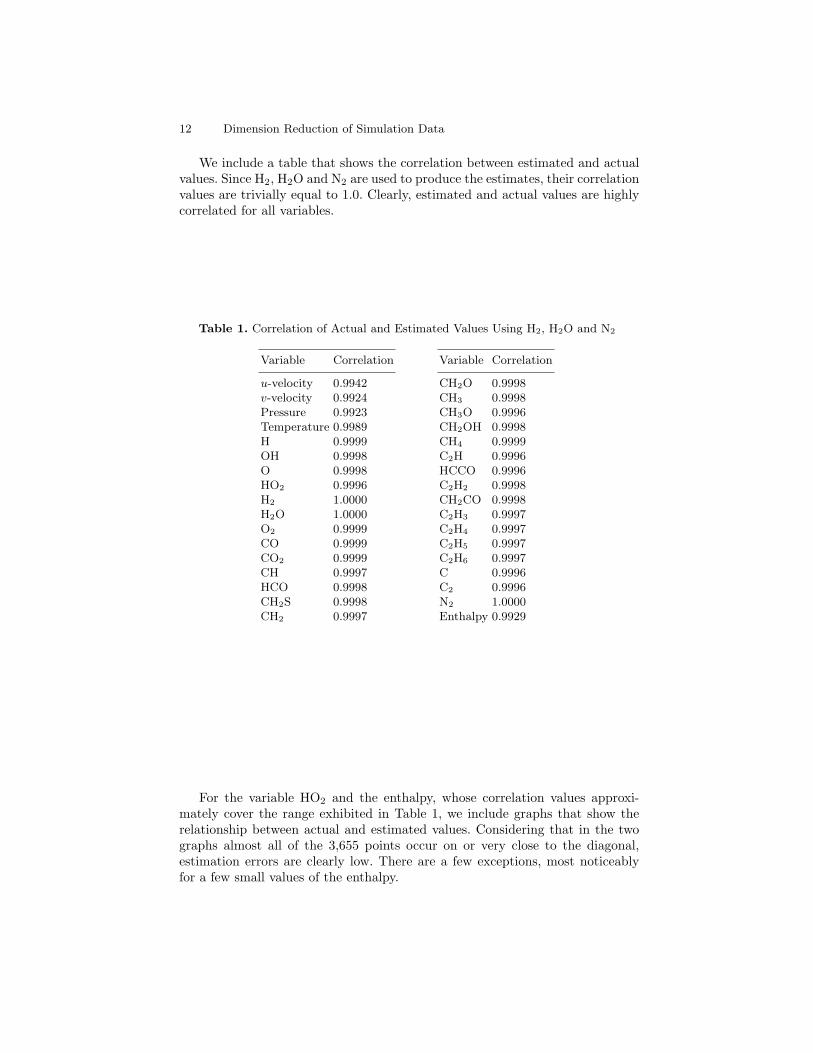
We include a table that shows the correlation between estimated and actualvalues. Since H2, H2O and N2 are used to produce the estimates, their correlationvalues are trivially equal to 1.0. Clearly, estimated and actual values are highlycorrelated for all variables.

Table 1. Correlation of Actual and Estimated Values Using H2, H2O and N2

Variable Correlation

u-velocity 0.9942v-velocity 0.9924Pressure 0.9923Temperature 0.9989H 0.9999OH 0.9998O 0.9998HO2 0.9996H2 1.0000H2O 1.0000O2 0.9999CO 0.9999CO2 0.9999CH 0.9997HCO 0.9998CH2S 0.9998CH2 0.9997


CH2O 0.9998CH3 0.9998CH3O 0.9996CH2OH 0.9998CH4 0.9999C2H 0.9996HCCO 0.9996C2H2 0.9998CH2CO 0.9998C2H3 0.9997C2H4 0.9997C2H5 0.9997C2H6 0.9997C 0.9996C2 0.9996N2 1.0000Enthalpy 0.9929

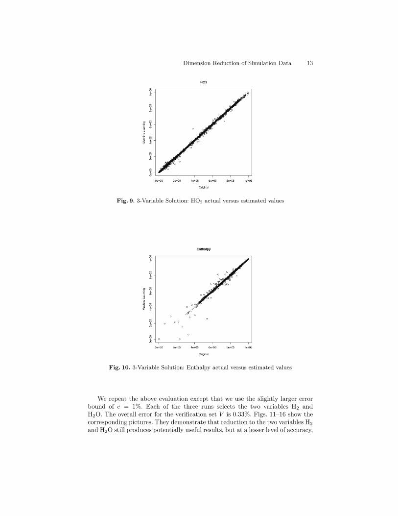
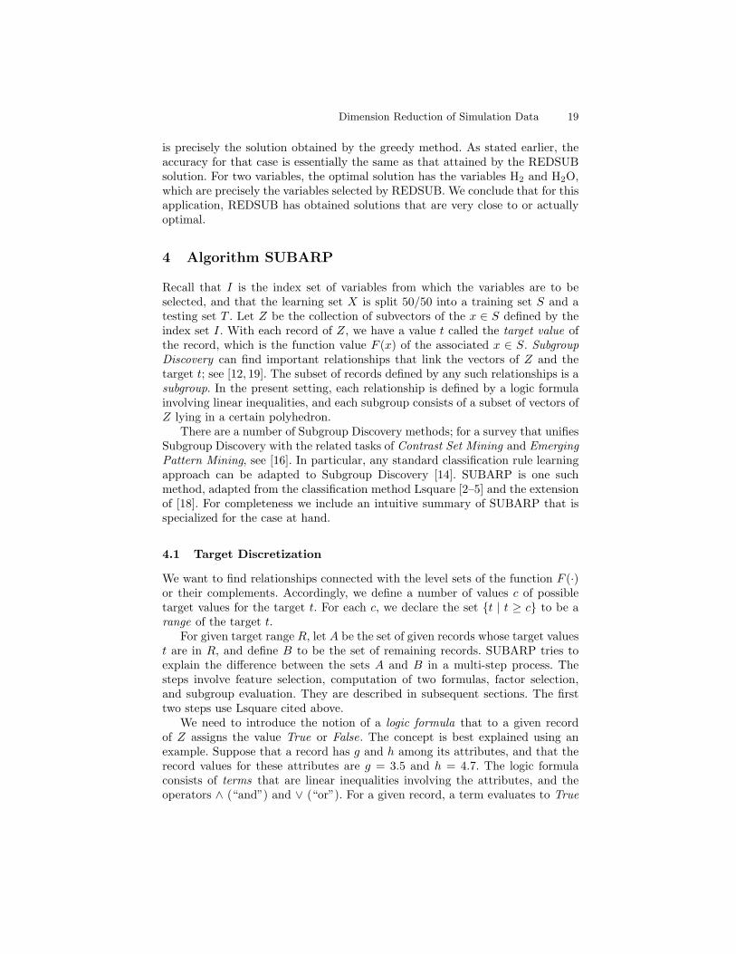
For the variable HO2 and the enthalpy, whose correlation values approxi-mately cover the range exhibited in Table 1, we include graphs that show therelationship between actual and estimated values. Considering that in the twographs almost all of the 3,655 points occur on or very close to the diagonal,estimation errors are clearly low. There are a few exceptions, most noticeablyfor a few small values of the enthalpy.


Fig. 9. 3-Variable Solution: HO2 actual versus estimated values

Fig. 10. 3-Variable Solution: Enthalpy actual versus estimated values

We repeat the above evaluation except that we use the slightly larger errorbound of e = 1%. Each of the three runs selects the two variables H2 andH2O. The overall error for the verification set V is 0.33%. Figs. 11–16 show thecorresponding pictures. They demonstrate that reduction to the two variables H2

and H2O still produces potentially useful results, but at a lesser level of accuracy,


as is evident from occasional and moderate disparities of the color patterns onthe left-hand side versus the right-hand side.

In agreement with the results shown for the 3-variable case, we also includea table showing the correlation of actual and estimated values for all variablesand enthalpy, and two graphs providing details for HO2 and enthalpy.

The reader may wonder whether a much simpler approach could producethe same results. For example, a greedy method could use in each iterationminimum average error computed by the Lazy Learner als deletion criterionand thus would avoid the subgroup discovery process. We have implementedthat method and obtained the following results. First, for the case of e = 0.5%,the simplified process obtains a solution with the three variables OH, H2, andO2. The overall error is virtually identical to that obtained earlier, 0.25% nowversus 0.26% earlier. But for e = 1%, the simplified method finds a solutionwith the two variables H2 and O2. The average error turns out to be 0.94%,which is almost triple of the 0.33% error for the earlier derived solution with twovariables. Indeed, the solution obtained by the simplified method is essentiallyunusable.

Fig. 11. 2-Variable Solution: Accuracy for C2H2


Fig. 12. 2-Variable Solution: Accuracy for CH4

Fig. 13. 2-Variable Solution: Accuracy for CO


Fig. 14. 2-Variable Solution: Accuracy for HCO

Fig. 15. 2-Variable Solution: Accuracy for Enthalpy


Fig. 16. 2-Variable Solution: Accuracy for Temperature

Table 2. Correlation of Actual and Estimated Values Using H2 and H2O


u-velocity 0.9942v-velocity 0.9890Pressure 0.9845Temperature 0.9988H 0.9999OH 0.9997O 0.9998HO2 0.9996H2 1.0000H2O 1.0000O2 0.9997CO 0.9999CO2 0.9996CH 0.9997HCO 0.9998CH2S 0.9998CH2 0.9997


CH2O 0.9998CH3 0.9998CH3O 0.9996CH2OH 0.9998CH4 0.9663C2H 0.9997HCCO 0.9996C2H2 0.9998CH2CO 0.9998C2H3 0.9997C2H4 0.9998C2H5 0.9997C2H6 0.9997C 0.9996C2 0.9996N2 0.9519Enthalpy 0.9881


Fig. 17. 2-Variable Solution: HO2 actual versus estimated values

Fig. 18. 2-Variable Solution: Enthalpy actual versus estimated values

How close are the two solutions obtained above for two and three variables tooptimal solutions with the same number of variables, assuming that the averageerror computed by the Lazy Learner is to be minimized? Since the number ofvariables is small, the question can be settled by enumeration of cases. For the3-variable case, the optimal solution has the variables OH, H2, and O2, which


is precisely the solution obtained by the greedy method. As stated earlier, theaccuracy for that case is essentially the same as that attained by the REDSUBsolution. For two variables, the optimal solution has the variables H2 and H2O,which are precisely the variables selected by REDSUB. We conclude that for thisapplication, REDSUB has obtained solutions that are very close to or actuallyoptimal.

4 Algorithm SUBARP

Recall that I is the index set of variables from which the variables are to beselected, and that the learning set X is split 50/50 into a training set S and atesting set T . Let Z be the collection of subvectors of the x ∈ S defined by theindex set I. With each record of Z, we have a value t called the target value ofthe record, which is the function value F (x) of the associated x ∈ S. SubgroupDiscovery can find important relationships that link the vectors of Z and thetarget t; see [12, 19]. The subset of records defined by any such relationships is asubgroup. In the present setting, each relationship is defined by a logic formulainvolving linear inequalities, and each subgroup consists of a subset of vectors ofZ lying in a certain polyhedron.

There are a number of Subgroup Discovery methods; for a survey that unifiesSubgroup Discovery with the related tasks of Contrast Set Mining and EmergingPattern Mining, see [16]. In particular, any standard classification rule learningapproach can be adapted to Subgroup Discovery [14]. SUBARP is one suchmethod, adapted from the classification method Lsquare [2–5] and the extensionof [18]. For completeness we include an intuitive summary of SUBARP that isspecialized for the case at hand.

4.1 Target Discretization

We want to find relationships connected with the level sets of the function F (·)or their complements. Accordingly, we define a number of values c of possibletarget values for the target t. For each c, we declare the set {t | t ≥ c} to be arange of the target t.

For given target range R, let A be the set of given records whose target valuest are in R, and define B to be the set of remaining records. SUBARP tries toexplain the difference between the sets A and B in a multi-step process. Thesteps involve feature selection, computation of two formulas, factor selection,and subgroup evaluation. They are described in subsequent sections. The firsttwo steps use Lsquare cited above.

We need to introduce the notion of a logic formula that to a given recordof Z assigns the value True or False. The concept is best explained using anexample. Suppose that a record has g and h among its attributes, and that therecord values for these attributes are g = 3.5 and h = 4.7. The logic formulaconsists of terms that are linear inequalities involving the attributes, and theoperators ∧ (“and”) and ∨ (“or”). For a given record, a term evaluates to True


if the inequality is satisfied by the attribute values of the record, and evaluates toFalse otherwise. Given True/False values for the terms, the formula is evaluatedaccording the standard rules of propositional logic.

For example, (g ≤ 4) and (h > 3) are terms. A short formula using theseterms is (g ≤ 4) ∧ (h > 3). For the above record with g = 3.5 and h = 4.7, bothterms of the formula evaluate to True, and hence the formula has that value aswell. As a second example, (g ≤ 4) ∨ (h > 5) produces the value True for thecited record, since at least one of the terms evaluates to True.

4.2 Feature Selection

This step, which is handled by Lsquare, repeatedly partitions the set A intosubsets A1 and A2; correspondingly divides the set B into subsets B1 and B2;finds a logic formula that achieves the value True on the records of A1 and Falseon those of B1; and tests how often the formula achieves True for the recordsA2 and False for those of B2. In total, 20 formulas are created. In Lsquare,these formulas are part of an ensemble voting scheme to classify records. Here,the frequency with which a given attribute occurs in the formulas is used as anindicator of the importance of the attribute in explaining the differences betweenthe sets A and B. Using that indicator, a significance value is computed for eachattribute. The attributes with significance value beyond a certain threshold areselected for the next step.

4.3 Computation of Two Formulas

Using the selected attributes, Lsquare computes two formulas. One of the for-mulas evaluates to True for the records of A and to False for those of B, whilethe second formula reverses the roles of A and B.

Both formulas are in disjunctive normal form (DNF), which means that theyconsist of one or more clauses combined by “or.” In turn, each clause consists oflinear inequality terms as defined before and combined by “and.” An example ofa DNF formula is ((g ≤ 4)∧ (h > 3))∨ ((g < 3)∧ (h ≥ 2)), with the two clauses((g ≤ 4) ∧ (h > 3)) and ((g < 3) ∧ (h ≥ 2)). Later, we refer to each clause as afactor.

Next, using the general construction approach of [14], we derive factors, andthus implicitly subgroups, from the first DNF formula. The same process iscarried out for the second DNF formula, except for reversal of the roles of A andB.

4.4 Factor Selection

Recall that the first DNF formula evaluates to False for the records of B. Letf be a factor of that formula. Since the formula consists of clauses combinedby “or,” the factor f also evaluates to False for all records of B. Let Q be thesubset of records for which f evaluates to True. Evidently, Q is a subset of A.


We introduce a direct description of Q using an example. Suppose the factorf has the form f = ((g ≤ 4)∧ (h > 3). Let us assume that A was defined as thesubset of records for which the values of target t fall into the range R = {t ≥ 9}.Then Q consists of the records of the original data set satisfying t ≥ 9, g ≤ 4, andh > 3. But we know more than just this characterization. Indeed, each recordof B violates at least one of the inequalities g ≤ 4 and h > 3. Put differently,for any record where t does not satisfy t ≤ 9, we know that at least one of theinequalities g ≤ 4 and h > 3 is violated.

So far, we have assumed that the formula evaluates to False for all recordsof B. In general, this goal may not be achieved, and the formula produces thedesired False values for most but not all records of B. Put differently, Q thencontains a few records of B. For the above example, this means that for somerecords where the target t does not satisfy t ≥ 9, both inequalities x ≤ 4 andy > 3 may actually be satisfied.

Potentially, the target range R and the factor f characterize an importantconfiguration that corresponds to an interesting and useful subgroup. On theother hand, the information may be trivial and of no interest. To estimate whichcase applies, SUBARP computes a significance value for each factor that lies inthe interval [0, 1]. The rule for computing the significance value is related to thoseused in other Subgroup Discovery methods, where the goal of interestingness [13]is measured with quality functions balancing conflicting goals such as (1) the sizeof the subgroup, (2) the length of the pattern or rule defining the subgroup, and(3) the extent to which the subgroup is contained in the set A. Specifically,SUBARP decides significance using the third measure and the probability withwhich a random process could create a set of records M for which the target t isin R, the factor f evaluates to True, and the size of M matches that of Q. Wecall that random process an alternate random process (ARP).

Generally, an ARP is an imagined random process that can produce an in-termediate or final result of SUBARP by random selection. SUBARP considersand evaluates several ARPs within and outside the Lsquare subroutine, and thenstructures decisions so that results claimed to be important can only be achievedby the ARPs with very low probability. The overall effect of this approach is thatsubgroups based on factors with very high significance usually turn out to beinteresting and important.

Up to this point, the discussion has covered polyhedra representing subgroupscontained in a level set. When the same computations are done with the roles ofA and B reversed, polyhedra are found that represent subgroups contained inthe complement of a level set. It is easily seen that the arguments made earlierabout the importance of variables based on the earlier polyhedra apply as wellwhen the latter polyhedra are used.

4.5 Evaluation of Subgroups

Once the significance values have been computed for the subgroups, the associ-ated target ranges and factors are used to compute a second significance valueusing the testing records of T , which up to this point have not been employed


by SUBARP. The average of the significance values obtained from the trainingand testing data is assigned as overall significance value to each subgroup.

In numerous tests of data sets, it has turned out that only subgroups withvery high significance value are potentially of interest and thus may produce newinsight. Based on these results, only subgroups with significance above 0.90 areconsidered potentially useful.

Finally, we relate the output of highly significant subgroups to the originalproblem.

4.6 Interpretation of Significant Subgroups

Let f be the factor of a very significant subgroup and R = t ≥ c be the asso-ciated target range. Define P to be the polyhedron defined by P = {xj , j ∈ I |factor f evaluates to True}. Then the polyhedron is an important partial char-acterization of the level set {x | F (x) ≥ c} of the function F (·). As discussed inSection 2, the variables used in the definition of P can therefore be considered animportant part of the characterization of that level set. That fact supports theconstruction of the sets Ji described in Section 2 according to the frequencies qj

with which each variable xj , j ∈ I, occurs in the definitions of the polyhedra ofvery significant subgroups.

5 Summary

This paper introduces a method called REDSUB for the reduction of combustionsimulation models. REDSUB is based on the Machine Learning techniques ofSubgroup Discovery and Lazy Learner. Use of the method does not require anyuser-specified transformations of simulation data or other manual effort. Theeffectiveness of REDSUB is demonstrated with simulation data of a methane/aircombustion process, where 34 variables representing 29 chemical species of thecombustion mixture, 3 thermodynamic properties, and 2 velocity components arereduced to 3 variables. For the remaining 31 variables, the values are estimatedwith good accuracy over the entire range of possible values. An even smallermodel using 2 variables still has reasonable accuracy.

References

1. C. G. Atkeson, A. W. Moore, and S. Schaal. Locally weighted learning. ArtificialIntelligence Review, 11:11–73, 1997.

2. S. Bartnikowski, M. Granberry, J. Mugan, and K. Truemper. Transformation ofrational and set data to logic data. In Data Mining and Knowledge DiscoveryApproaches Based on Rule Induction Techniques. Springer, 2006.

3. G. Felici, F. Sun, and K. Truemper. Learning logic formulas and related errordistributions. In Data Mining and Knowledge Discovery Approaches Based onRule Induction Techniques. Springer, 2006.

4. G. Felici and K. Truemper. A MINSAT approach for learning in logic domain.INFORMS Journal of Computing, 14:20–36, 2002.


5. G. Felici and K. Truemper. The lsquare system for mining logic data. In Ency-clopedia of Data Warehousing and Mining, pages 693–697. Idea Group Publishing,2005.

6. R. Hilbert, F. Tap, H. El-Rabii, and D. Thevenin. Impact of detailed chemistryand transport models on turbulent combustion simulations. Progress in Energyand Combustion Science, 30:61–117, 2004.

7. A. E. Hoerl. Application of ridge analysis to regression problems. Chemical Engi-neering Progress, 58:54–59, 1962.

8. A. E. Hoerl and R. W. Kennard. Ridge regression: Biased estimation for nonorthg-onal problems. Technometrics, 12:55–67, 1970.

9. G. Janiga, O. Gicquel, and D. Thevenin. High-resolution simulation of three-dimensional laminar burners using tabulated chemistry on parallel computers. In2nd ECCOMAS Thematic Conference on Computational Combustion, 2007.

10. G. Janiga, A. Gordner, H. Shalaby, and D. Thevenin. Simulation of laminar burn-ers using detailed chemistry on parallel computers. In European Conference onComputational Fluid Dynamics (ECCOMAS CFD 2006), 2006.

11. G. Janiga and D. Thevenin. Three-dimensional detailed simulation of laminarburners on parallel computers. In Proceedings of the European Combustion MeetingECM2009, 2009.

12. W. Klosgen. EXPLORA: A multipattern and multistrategy discovery assistant. InAdvances in Knowledge Discovery and Data Mining. AAAI Press, 1996.

13. W. Klosgen. Subgroup discovery. In Handbook of Data Mining and KnowledgeDiscovery. Oxford University Press, 2002.

14. N. Lavrac, B. Cestnik, D. Gamberger, and P. Flach. Decision support throughsubgroup discovery: Three case studies and the lessons learned. Machine Learning,57:115–143, 2004.

15. T. Mitchell. Machine Learning. McGraw Hill, 1997.16. P. K. Novak, N. Lavrac, and G. I. Webb. Supervised descriptive rule discovery: A

unifying survey of contrast set, emerging pattern and subgroup mining. Journalof Machine Learning Research, 10:377–403, 2009.

17. N. Peters. Turbulent Combustion. Cambridge University Press, 2000.18. K. Truemper. Improved comprehensibility and reliability of explanations via re-

stricted halfspace discretization. In Proceedings of International Conference onMachine Learning and Data Mining (MLDM 2009), 2009.

19. S. Wrobel. An algorithm for multi-relational discovery of subgroups. In Proceed-ings of First European Conference on Principles of Data Mining and KnowledgeDiscovery, 1997.

dimension reduction of chemical process simulation data

Documents