Dilution effects, population growth and economic growthunder human capital accumulation and endogenous technological change

by Alberto Bucci, Levent Eraydın, Moritz Müller

No. 113 | JANUARY 2018

WORKING PAPER SERIES IN ECONOMICS

KIT – Die Forschungsuniversität in der Helmholtz-Gemeinschaft econpapers.wiwi.kit.edu

Impressum

Karlsruher Institut für Technologie (KIT)

Fakultät für Wirtschaftswissenschaften

Institut für Volkswirtschaftslehre (ECON)

Kaiserstraße 12

76131 Karlsruhe

KIT – Die Forschungsuniversität in der Helmholtz-Gemeinschaft

Working Paper Series in Economics

No. 113, January 2018

ISSN 2190-9806

econpapers.wiwi.kit.edu

Dilution Effects, Population Growth and Economic Growth

under Human Capital Accumulation and Endogenous

Technological Change∗

Alberto Bucci †, Levent Eraydın‡, Moritz Muller§

Abstract

This paper answers the following two questions: 1) In the data, can we find adilution effect of population growth also on per-capita human capital investment?If yes, 2) how can we use this fact to explain theoretically the existence of a dif-ferential impact of population change on economic growth across countries? In thefirst part of the article we document empirically the considerable across-countriesheterogeneity of a dilution effect of population growth also in regard to the pro-cess of per-capita human capital formation and observe that, at a country’s level,population growth may be relevant (either positively or negatively) for economicgrowth depending on the specific way it affects the process of schooling-acquisitionby agents. In the second part of the paper we use these results in order to builda multi-sector growth model which is capable of accounting (depending on thestrength of the found dilution effect of population growth on per-capita humancapital formation) for the non-monotonous correlation between demographic andeconomic growth rates in the long-run.

Keywords: Human Capital Investment, Economic Growth, Population Growth,Dilution Effects, Research & Development

JEL classification: J10, J24, O33, O41

∗The authors gratefully acknowledge the comments and suggestions of participants in the Conference“Finance and Economic Growth in the Aftermath of the Crisis” in Milan, Italy, and those of theparticipants in “KIT-BETA Workshops” held in University of Strasbourg, France. In addition, we wishto thank for the support by the Chair in Economic Policy, ECON, KIT, Germany.†Department of Economics, Management and Quantitative Methods (DEMM), University of Milan,

Italy, e-mail: alberto.bucci@unimi.it‡Corresponding author. Chair in Economic Policy, Institute of Economics (ECON), Karlsruhe In-

stitute of Technology, Germany, e-mail: levent.eraydin@kit.edu§Faculty of Economics and Management, University of Strasbourg, France, e-mail:

mueller@unistra.fr

1

1. Introduction

Because the existence of a causal relationship and, eventually, the sign of such a relationare still controversial issues in the literature, it remains very important (not only fordemographers and economists, but also for policy-makers) to investigate the impactthat population growth may have on long-term economic growth (i.e., the growth rateof real per-capita income). Many studies (Solow, 1956; Coale and Hoover, 1958; Ehrlich,1968; Li and Zhang, 2007; Herzer et al., 2012, just to mention a few) find a negativeinfluence of population growth on economic growth. In exogenous growth models, forexample, this result is ultimately explained by the so-called physical capital dilutioneffect of population growth: an increase in population, by diluting the stock of physicalcapital held by each individual, lowers ceteris paribus the long-run (or steady-state) leveland the short-run (or transitional) growth rate of physical capital per capita. Otherstudies (Kuznets, 1967; Boserup, 1981; Simon, 1981; Romer, 1987 and 1990; Kremer,1993; Jones, 1995), instead, conclude that, once endogenous technological change isexplicitly taken into account, the impact of population growth on economic growthis definitely positive as larger populations can stimulate the advancement of technicalprogress, are able to enjoy greater economies of scale, and are likely to have a greaternumber of geniuses. Finally, there are also strong arguments advocating that it is abetter economic performance (i.e., a higher economic growth rate) to cause an increasedpopulation growth rate.1 Blanchet (1988) is among those who years ago have alreadyused this claim to explain the presence of an insignificant correlation between economicand population growth rates.

In the light of all this, it seems that the main conclusion coming from the path-breaking paper by Kelley and Schmidt (1995, p. 554) still continues to hold today:“...This analysis...provides a more balanced perspective on the consequences of demo-graphic change because it rests on the proposition that population growth has both nega-tive and positive effects... As this paper demonstrates, population growth is not all goodor all bad for economic growth: it contains both elements, which can and...do changeover time”.

The present paper is motivated by empirical and theoretical reasons. More con-cretely, the two questions that our work tries to answer are, respectively, the following:In the data, is the so-called dilution effect of population growth (that the literatureoften relates solely to the process of per-capita physical capital accumulation) capableof influencing also the evolution over time of per-capita human capital? If yes, howcould we use this information to explain theoretically the existence of a differentialcross-country impact of population change on economic growth?

In the first part of our paper we investigate and document empirically the existence(and the considerable across-countries heterogeneity) of a dilution effect of populationgrowth also in regard to the process of per-capita human capital formation. More im-portantly, we also observe that, at a country’s level, population growth may be relevant(either positively or negatively) for economic growth depending on the specific way it(population growth) affects the process of schooling-acquisition by agents.

As a consequence of these empirical results, in the second part of the paper weturn to the theory and propose a generalization of the very well-known Uzawa (1965)’sand Lucas (1988)’s models. Our contribution introduces two important differenceswith respect to Uzawa (1965) and Lucas (1988). First of all, we assume that firms

1See Chang et al. (2014) for a recent empirical analysis that confirms this result.

2

may undertake horizontal R&D activity. This means that disembodied technologicalprogress (intended as the growth rate of the available varieties of intermediate inputs)is endogenous in our economy, as in the path-breaking papers by Romer (1990) andJones (1995). Moreover, and inspired by our empirical findings, we also postulate thatindividual human capital investment is subject to some sort of dilution effect relatedto an increase in population. According to this effect, since newborns enter the worldcompletely uneducated, they reduce the stock of human capital per-capita availablein the population. Hence, population growth operates like a depreciation of humancapital per capita and, thus, contributes to slow down human capital accumulation atan individual’s level. In the original Lucas (1988, Eq. 13, p. 19)’s model such a dilutioneffect in per-capita human capital investment is totally missing, based on the belief thatskill acquisition is a sort of “social activity” and, as such, it is completely different fromphysical capital investment.2

Our extended model shows that the magnitude of the dilution effect of populationchange on per-capita human capital investment can be used as an argument to explainthe differential (i.e., positive, negative, or neutral) impact that population growth mayhave on long-run economic growth across countries. In other words, our theoreticalmodel can be employed to propose a new, alternative explanation as to the non-uniformeffect of population growth on long-run per capita income growth. This new explanationis based on the recognition that population growth brings about two simultaneous,but different (in sign and size), effects on economic growth. The first is precisely thealready-mentioned dilution effect. This effect is always negative because when newbornsenter the world they reduce the existing per-capita stock of any reproducible factor-input (human capital in our case). So, in order to equip every single member of thegrowing population with an even amount of such input, some further resources needto be explicitly devoted to this aim (as opposed to other, alternative/more productiveuses), which slows productivity growth down. The second effect, instead, describesthe positive impact that population growth may have on the economy’s growth rate ofideas,3 and hence on per-capita income growth. What our theoretical model ultimatelysuggests is then a mechanism such that there exists a country-specific threshold levelin the magnitude of the per-capita human capital accumulation dilution effect: forthose countries in which the dilution effect of population growth is below (above) thethreshold we should observe a positive (negative) impact of population change on long-run economic growth.

Although one contribution of the present paper is mainly empirical,4 we believe thatthe theoretical model we present in the second part of this article has features that make

2“...To obtain (13) for a family, one needs to assume both that each individual’s capital follows thisequation and that the initial level each new member begins with is proportional to (not equal to!) thelevel already attained by older members of the family. This is simply one instance of a general fact thatI will emphasize again and again: that human capital accumulation is a social activity, involving groupsof people in a way that has no counterpart in the accumulation of physical capital...”(Lucas, 1988, p.19).

3“...More people means more Isaac Newtons and therefore more ideas” (Jones, 2003, p. 505).4As far as we know, this is the first paper that attempts at estimating a dilution effect of population

growth on per-capita human capital formation, irrespective of the sources of the demographic change.Indeed, Boikos et al. (2013) estimate the effect that a change in the birth rate (as opposed to thewhole population growth rate) has on per-capita human capital investment. Moreover, in their modelBoikos et al. (2013) consider an economy where people do not save (aggregate output equals aggregateconsumption at all times), there is no R&D activity (and, hence, no endogenous disembodied techno-logical change), and in which the aggregate production function is linear in the only input employed,i.e. human capital.

3

it new and original within the existing literature. Unlike the canonical Romer (1990)’sand Jones (1995)’ settings, we consider the possibility that the intermediate sector useshuman capital as an input. Hence, in our model human capital is employed to producenew human capital, final and intermediate goods, and to invent new ideas. Despite thefact that in Mierau and Turnovsky (2014) — who use a one-sector endogenous growthframework a la Romer (1986) — the link between the whole population growth rateand the economic growth rate is monotonic, their model is still able to account fora hump-shaped relation between the two variables since population growth can be ex-plained by either an increase in fertility or a reduction in mortality. Thus, in Mierau andTurnovsky (2014) the way in which population growth occurs (i.e., through an increasein the birth rate or a decrease in the mortality rate) is important in making the rela-tionship between demographic change and economic growth ultimately non-uniform insign. Our paper differs from Mierau and Turnovsky (2014) in that we consider a multi-sector growth model with R&D activity and human capital accumulation. Moreover, wedo not split the population growth rate into its birth- and mortality-rate componentsbecause we are interested in uncovering another potential source of non-monotonicityin the overall relationship between demographic change and economic growth. Usingan endogenous growth model with human capital investment and two types of R&Dactivities (horizontal and vertical, respectively), Strulik (2005) concludes that the signof the correlation between population growth and the growth rate of per capita in-come crucially depends on the form of households’ preferences (‘Millian’, ‘Benthamite’,or an intermediate type between the two, respectively). By considering an economywhere R&D activity is purely horizontal, Bucci (2008), instead, postulates that the in-vestment in skill-acquisition by agents is directly influenced by technological progress.In his framework, the sign of the long-run correlation between population growth andeconomic growth is ultimately found to depend not only on the form of households’preferences, but also on the nature of technical change (whether ‘skill-biased’, ‘eroding’,or ‘neutral’). Unlike Bucci (2013), it is not an objective of this article to highlight therole of the so-called ‘returns-to-specialization’ in shaping the link between populationgrowth and economic growth. Moreover, contrary to Bucci (2008, 2013) and Strulik(2005), we pay no attention here to how the type of households’ preferences might con-tribute to affect the correlation between population and economic growth rates. Finally,differently from Bucci (2015), in the present article we are not interested in highlightingthe possible tension between productivity-gains (due to specialization) and productivity-losses (due to production-complexity) that arises from an expansion of input-variety asa major determinant of the sign of the long-run relation between economic and popula-tion growth rates. Instead, as mentioned above, we are interested here in emphasizinga totally new mechanism (based on the role played by the dilution effect of populationchange on human capital formation by agents) through which the relation between pop-ulation and economic growth rates might be non-uniform in sign in the long-term. In arecent paper, Prettner (2014) has proposed another way through which a higher pop-ulation growth can have a non-monotonous effect on economic growth within a Romer(1990)’s—Jones (1995)’s economy augmented with an education sector: in his model,an increase in population growth, while positively influencing aggregate human capitalaccumulation, decreases simultaneously schooling intensity (defined as the productivityof teachers times the resources spent on educating each child). The fall of schoolingintensity has, in turn, a negative impact on the future evolution of aggregate humancapital. Depending on whether this negative effect of population growth dominates onthe positive one or not, we can ultimately observe a non-uniform impact of population

4

change on economic growth in the long-run. Prettner (2014), however, is not interestedin emphasizing the role of the dilution effect in per capita human capital investment,which is instead the main focus of our article.

The remainder of the paper is organized as follows. Section 2 empirically estimatesthe effects of population growth on economic growth through individuals’ human cap-ital formation. Section 3 lays out the theoretical model, and Section 4 analyzes itspredictions along a Balanced Growth Path (BGP henceforth) equilibrium. Section 5focuses on the correlation between population growth and per-capita income growthin the long-run, and explains the possibly non-monotonous sign of this correlation interms of the extent of a dilution effect of population growth on per-capita human capi-tal accumulation. The last Section concludes and provides grounds for possible futureextensions.

2. Population growth, human capital formation and eco-nomic growth: An empirical investigation

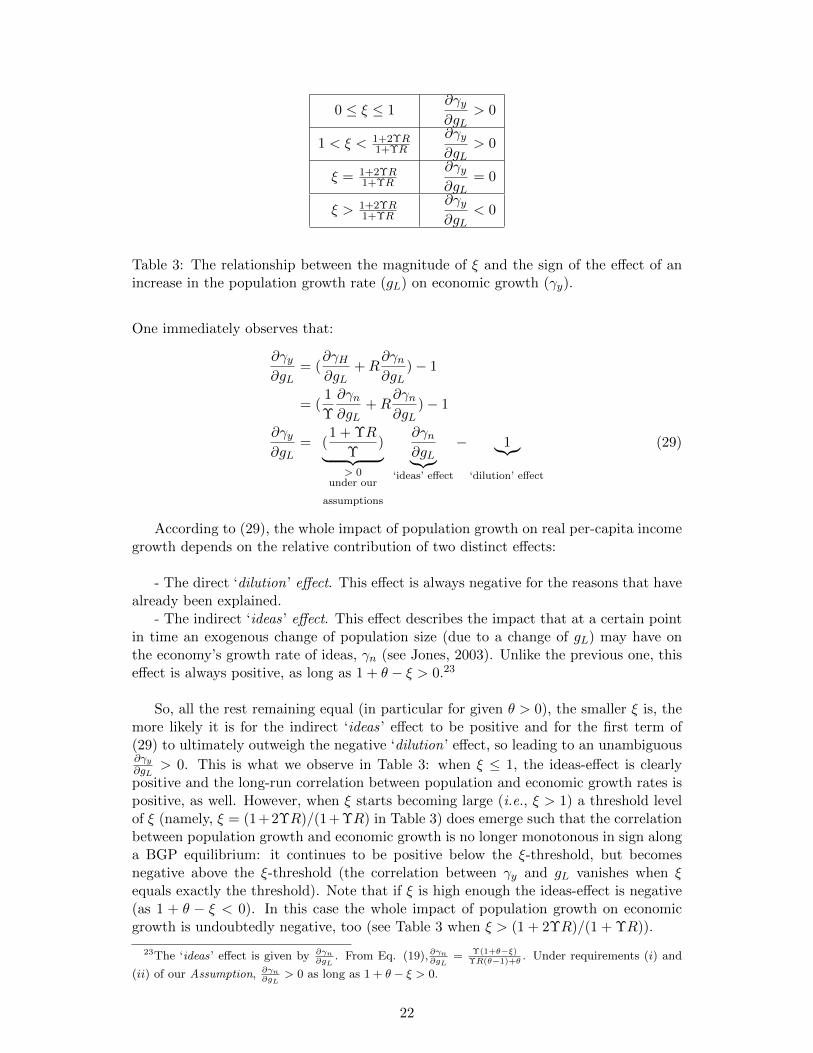
This section consists of two parts. The first part investigates the relationship betweenpopulation growth and human capital formation. The second part considers the impactof both population growth and human capital on long-run economic growth. In order tocapture all these dimensions, we use population data from the United Nations (2015),the schooling attainment data of Barro and Lee (2013), and GDP data from the PennWorld Tables (Feenstra et al., 2013).

Our sample excludes countries from East Europe, Central Asia, and Germany be-cause of their transition from non-market to market economies during the 1980s and1990s, and we exclude countries for which we have missing information from 1960 on-wards. Furthermore, five outliers in terms of schooling are excluded from the sample.These restrictions leave us with 92 countries across five world regions.5

Population growth in a given year is measured as the natural population growthrate, i.e. crude birth rate minus crude death rate in that year, not taking into accountthe migration rate. Migration effects on human capital and economic growth are thusignored in the analysis. Following the literature, we measure human capital in terms of(logged) years of schooling.6 Economic wealth is measured in terms of (logged) output-side real GDP at chained PPPs. In the schooling regression we normalize GDP by thesize of the population aged above twenty in order to separate this measure from thepopulation growth rate, while in the long-run economic growth regression we normalizeby the total size of the population to arrive at GDP per capita. Long-run economicgrowth is the difference of log GDP per capita over the time period.

In a first step, we investigate how population growth relates to years of school-ing. The prior literature generally suggests that the impact of population growth onschooling may greatly vary across economies and over time (Bloom et al., 2000; Bloom

5See appendix A1 for the list of countries and descriptive statistics by region and year.6The advantage of years of schooling is that it is relatively easy to measure and it is a clear policy

variable. On the other hand, schooling as a measure of human capital has been increasingly criticized asit is not a direct measure of human capital but rather one of several inputs to human capital formation,informing on quantity and not on quality of schooling. There have been various attempts to overcomethese limitations, notably considering students’ cognitive skills as evaluated in international tests (e.g.Hanushek and Woessmann, 2008). This approach however has its own drawbacks. It considers onlychildren actually being in school, results in very broad skill distributions that are relatively unstableover time within countries, and are difficult to compare across countries.

5

et al., 2010; Kelley, 1994; Montgomery et al., 2000). More specifically, Boikos et al.(2013) investigate the effect of fertility rates on schooling and find an inverse-U-shapedrelationship. Furthermore, population growth realized through higher life expectancyis likely to have a positive impact on educational attainment (see e.g. Cervellati andSunde, 2013). In general, population growth can be expected to be more relevant inresource-constrained environments where the schooling decision depends stronger onthe (changes of) resources available per child (Kelley, 1994). In addition, incentives foreducation depend on the economic structure of the economy. It has been argued for ex-ample that in South Korea, during the 1980s, population growth through larger cohortsof the younger generation resulted in an increase of secondary and tertiary education asa rational response to increased competition for jobs in the growing high-tech industry(Kim, 2001). On the other hand, population growth in China during the 1980s didnot result in comparable schooling because of severe resource constraints of the house-holds in combination with a strong expansion of the low-skilled manufacturing sector(Li et al., 2017; Liu et al., 2009). Finally, population growth effects probably dependon education policy. Consider for example Kelley (1994)’s argument that populationgrowth may impact schooling attainment even positively in cases where it increases thepressure on policy to implement appropriate education reforms towards higher efficiencyin the education sector.

The schooling regression follows a production logic, where the schooling of theyounger cohort is a function of the schooling of the adults, the GDP available to theadults, and population growth. The dependent variable is measured at the year whenthe younger cohort reached age 25 to 29 years, when schooling is mostly over. All in-dependent variables are measured however twenty years earlier, when the cohort of theyoung has been 5 to 9 years old — at a time or before when most schooling decisions areactually made. We estimate one regression over consecutive five-year periods startingfrom 1960 until 1990. This time period is due to the gap of 20 years between the timewhen the education decision was made, e.g. 1990, and the time where we observe thefinal outcome of that decision, e.g. 2010.

The structure of the model is as follows:

syi,t = ci + βixi,t + τt + εi,t with ci = δxi,0 + ui(uiβi

)∼ N

((0β

),Ω

)In the first equation, schooling of the young, syi,t depends on an intercept, ci, various

time-varying and constant regressors xi,t, time dummies τt and a random error termεi,t. The model allows for country specific intercept ci and slope βi.

We may expect that ci correlates with xi,t. The second equation implements acorrelated random coefficients approach as it explicitly models the correlation betweenci and the country’s initial conditions xi,0. The time constant, country-specific errorterm ui can then be assumed to be uncorrelated with the right-hand side variables ofthe first equation.7 In the estimation, the second equation is simply plugged into the

7The more common approach of controlling through averages of the regressors (rather than initialvalues) in our case provides very similar results but is less appropriate. First, it is reasonable thatregressors are weakly and not strongly independent and, second, schooling of the adults is a stock builtthrough schooling of the young. Both issues introduce (some) correlation between regressor averagesand the error term εi,t. Estimation in first differences is an alternative that suffers from the same

6

first equation - yielding a simple linear regression with additional country averages ascontrols (Hsiao, 2003, pp.44).

Heterogeneous slopes βi can not be identified for each country individually. However,a random effects approach allows to obtain an estimate of the distribution of βi under theassumption that εi,t, ui, and βi are independent from regressors and follow a Normaldistribution. The corresponding mean, i.e. average fixed effects β, and covariancematrix, Ω, are then freely estimated.8

As we measure independent variables before the outcome realizes reverse causality— better educated have less kids — is not an issue. One may argue however thatforward-looking, rational parents decide simultaneously on the number of children andassociated schooling investments (Becker and Lewis, 1973). Typically it is assumed thatsuch a decision involves a trade-off leading to more (fewer) children with lower (higher)education. Our estimation approach results into stronger (negative) population growtheffects in economies where these considerations are more relevant. We further note thatestimates of population growth coefficients remain subject to an omitted variables bias:Population growth is one of several dimensions reflecting the socio-economic state ofan economy and hence is susceptible of taking over explanatory power from related butdifferent factors that are not included in the regression. Consequently, we rather speakof correlations than causal effects in the following.

Table 1 presents the results of our schooling regressions. Model (1) presents first-difference panel estimates of our main variables as a base line model. Model (2) providesestimates implementing the correlated random coefficients approach in combination witha linear mixed model. Model (1) and (2) are two alternative approaches of dealing withcountry-specific (fixed) effects. Only the intercept and R2 change considerably as we gofrom the estimation in differences (Model 1) to estimation in levels (Model 2). Despitethat coefficient estimates are very similar in both models. Note that all factors enterwith a curvilinear slope. In particular population growth follows an inverse-U-shapewith an optimal point slightly above two percent population growth, which is consistentwith (Boikos et al., 2013).

Model (3) allows for random country-specific coefficients of schooling and GDP ofadults. Moving from Model (2) to (3) improves model fit significantly according to thelikelihood ratio test, and while the marginal R2 (based on fixed effects only) decreases,the conditional R2 (based on fixed and random effects) increases. Population growthcoefficient estimates remain very stable but become somewhat more precise.

The final model, Model (4), includes country-specific population growth effects. Wenote that coefficients do not change much compared to their standard deviations. Yet,the likelihood ratio test strongly rejects equivalence of Model (4) and Model (3) in termsof data fit. Similarly, conditional R2, taking into account estimated random interceptand slopes increases. These results strongly suggest considerable heterogeneity acrosscountries in terms of the effect of population growth on schooling.

issues. Furthermore, differencing reduces the signal-to-noise ratio considerably in case measurementerrors are uncorrelated over time, which is likely to be the case in our data (Cohen and Soto, 2007).For comparison, we provide nevertheless first-difference results in the main regression table.

8We also estimated simple OLS regressions in which we allow the population growth effect to varyover world regions (instead of individual countries) and obtained results that are consistent with theones presented here.

7

Tab

le1:

Est

imat

esof

the

impac

tof

pop

ula

tion

grow

thon

sch

ool

ing

ofth

eyo

un

gfr

om

1960

to1990.

(1)

(2)

(3)

(4)

Com

mon

effec

tsIn

terc

ept

0.07

2***

(0.0

07)

0.3

3*

(0.1

33)

0.3

19*

(0.1

55)

0.3

76*

(0.1

67)

Sch

ool

ing

adu

lts

1.71

***

(0.4

05)

1.7

64***

(0.2

88)

2.1

68***

(0.3

29)

2.0

07***

(0.3

53)

(Sch

ool

ing

adu

lts)

2-0

.729

***

(0.1

72)

-0.6

61***

(0.1

23)

-0.8

49***

(0.1

39)

-0.7

76***

(0.1

49)

GD

Pp

.ad

ult

0.13

8**

(0.0

52)

0.2

66***

(0.0

43)

0.3

04***

(0.0

52)

0.2

88***

(0.0

54)

(GD

Pp

.ad

ult

)2-0

.036

**(0

.011

)-0

.058***

(0.0

1)

-0.0

59***

(0.0

11)

-0.0

54***

(0.0

11)

Pop

ula

tion

grow

th0.

093*

(0.0

38)

0.0

94**

(0.0

35)

0.1

07***

(0.0

29)

0.1

24***

(0.0

3)

(Pop

ula

tion

grow

th)2

-0.0

17(0

.009

)-0

.022**

(0.0

07)

-0.0

24***

(0.0

07)

-0.0

28***

(0.0

08)

Corr

elate

dra

ndom

inte

rcep

tco

ntr

ols

Init

ial

sch

ool

ing

—0.3

28***

(0.0

57)

0.1

89***

(0.0

44)

0.2

02***

(0.0

42)

Init

ial

GD

P19

60—

-0.0

02

(0.0

28)

0.0

3(0

.022)

0.0

23

(0.0

21)

Init

ial

Pop

ula

tion

grow

th19

60—

-0.0

21

(0.0

25)

-0.0

21

(0.0

18)

-0.0

27

(0.0

18)

Ran

dom

coeffi

cien

ts

Ω

In

terc

ept

Sch

ool

ing

adu

lts

Log

GD

Pp

.ad

ult

Pop

ula

tion

grow

th

(Pop

ula

tion

grow

th)2

—

0.1

2−

−−

−−

−−−−

−−−−−

0

.43

−0.

77

0.31

0.1

4−

0.74

0.1

3−

−−

−−

−−

−−

0.

56

−0.7

60.

32

−0.0

8−

0.58

0.13

0.03−

0.15

0.23

0.06

−0.3

80.

29−

0.02−

0.88

0.0

3

lo

gL

ikel

ihood

—458.7

8573.3

1606.1

7L

LR

test

χ2

=229.0

6,

DF

=5,

χ2

=65.7

36,

DF

=9,

p-v

al=<

0.01%

p-v

al=<

0.0

1%

Mar

gin

al/C

ond

itio

nalR

20.

158/

—0.8

52/0.9

36

0.7

77/0.9

64

0.7

64/0.9

73

Not

es:

All

regr

essi

ons

are

on92

obse

rvat

ion

san

din

clu

de

tim

ean

d“w

orl

dre

gio

n”

du

mm

ies.

Mod

el(1

)is

on

firs

t-d

iffer

ence

s,M

od

els

(2)

to(4

)on

level

s.L

ikel

ihood

rati

o(L

LR

)te

stst

atis

tics

for

equ

ival

ence

of

Mod

el(2

)an

dM

od

el(3

),an

dM

odel

(3)

and

Mod

el(4

)re

spec

tive

ly.

On

est

ar

den

ote

sth

e5%

,tw

ost

ars

1%,

and

thre

est

ars

0.1%

con

fid

ence

leve

ls.

Sta

nd

ard

erro

rsin

bra

cket

s.

8

Figure 1 plots observed population growth rates, g, against expected country-specific

effects of population growth on schooling, i.e. expectations of(∂sy

∂g

)conditional on the

estimated distribution. The figure shows the additional insight gained from allowingheterogeneity across countries in the effect of population growth on schooling.

0 1 2 3 4

-0.3

-0.2

-0.1

0.0

0.1

0.2

0.3

Population growth rate, g

Mar

gin

aleff

ect

onsc

hool

ing,( ∂sy ∂

g

)

Figure 1: Population growth rate, g, against its marginal effect on schooling, ∂sy

∂g , takinginto account fixed-common effects and random-individual effects (both averaged overyears for each country). Advanced economies in red, Asia in blue, Latin America andCaribbean in green, Middle East and North Africa in black, Sub-Saharan Africa inorange. The black line marks the estimated marginal effect based on fixed, commoneffects only.

First, the black line provides estimated marginal effects without heterogeneity, i.e.when the effect is allowed to vary only with population growth. The estimated inverse-U-shaped relationship implies decreasing marginal effects as population growth increases.Noticing that countries with low population growth are often more advanced countries,this pattern is in line with the argument that population growth has a particularly neg-ative effect on human capital formation in developing, resource-constrained economies.This finding is consistent with (Boikos et al., 2013).

Second, turning to country-specific marginal effects, we see that estimated marginaleffects of advanced economies (red triangles) are very close to the common effects es-timates (black line). However, for developing countries with higher population growthrate country-specific effects are widely dispersed around the common effects estimate.

Keeping population growth fixed, say at about 3 percent, some countries are ex-pected to experience a negative impact of population growth on schooling (such as theAfrican country in orange with ∂sy

∂g = −0.2) while others are at the other end of the

9

spectrum (see the Middle East country in black at ∂sy

∂g = 0.2). Furthermore, the spreadis considerable within ‘world regions’ for countries experiencing the same populationgrowth rate. The observed heterogeneity among even otherwise ‘similar’ countries maywell explain the ambiguity in the prior empirical literature regarding the dilution effectof population growth on human capital formation.

What is then the implication for economic growth? The second part of the analysisprovides some intuition based on a regression of long-run economic growth on popula-tion growth and years of schooling. We consider the period 1980 to 2010 — a period ofaccelerated skill biased technological change (Acemoglu, 2002) — where we expect hu-man capital to be a relevant mediator of the population-economic growth relationship.The idea is that population growth before the regression period influences schooling ofthe young, which in turn affects economic growth once they enter the labor force duringthe regression period. Following Benhabib and Spiegel (1994) we consider the averagelevel of human capital as a driver of growth in a catching-up process. The regression isthus on initial GDP per capita (logged) at 1980, average years of schooling in logs overthe regression period, and (natural) population growth rate in the prior period (1960to 1980).

Table 2: Long-run economic growth regression (1980-2010).

(1) (2) (3)

Intercept 1.448*** (0.285) 0.438 (0.336) -0.163 (0.43)GDP p.c. (1980) -0.203** (0.085) -0.407*** (0.083) -0.41*** (0.082)Avg. population growth -0.208** (0.09) -0.237*** (0.083) -0.234*** (0.084)Schooling (1980) 0.727*** (0.159)Avg. schooling 0.943*** (0.2)Asia 0.333 (0.205) 0.434** (0.204) 0.426** (0.2)Latin America 0.028 (0.184) 0.133 (0.182) 0.135 (0.183)Middle East / N. Africa 0.454* (0.258) 0.792*** (0.241) 0.759*** (0.238)S. Africa -0.596** (0.247) -0.324 (0.237) -0.33 (0.236)

Observations 92 92 92R2 0.457 0.568 0.572

Notes: Avg. population growth is the average over the period 1960 to 1980. Schooling refers toaverage years of schooling of the population in logs. Standard errors in brackets, always robustto heteroskedasticity and clustering within “world regions”. Model (1) and (2) estimated withOLS. Model (3) is a 2SLS regression with average schooling, i.e. log of schooling over theperiod 1980 to 2010, instrumented by schooling of the population in 1980, and schooling ofthe young (the dependent variable in the schooling regression) of the periods 1960 and 1965.F statistic of the first stage regression is 1108.93 and the test of weak Instruments rejects ata significance level below 0.01%. Sargan test p-value of 0.28, and Wu-Hausman test p-valueof 0.42.

Table 2 provides results of three regressions. Model (1) is without any schoolingvariable. We obtain a negative population growth effect that is significant below a 5%level. Model (2) increases initial schooling which increases the negative effect of avg.population growth and the estimate becomes more precise, but not much comparedto its standard error. GDP and regional dummy estimates tend to be more affected.Finally, Model (3) includes (instrumented) average years of schooling. Initial schoolingin Model (2) is substantial and highly significant, and we obtain an elasticity of one

10

for schooling in the final, our preferred, model. The coefficient of average populationgrowth remains very stable over all three models.

After controlling for schooling, we consider the negative coefficient of populationgrowth to be net of schooling, summarizing various other pathways. Note that theeffect of introducing schooling in the regression on our population growth rate estimateis rather small. But this can be expected given the results of the first regression that,in average, population growth has a negligible impact on schooling of the young. Yet,the schooling regression lets us expect considerable heterogeneity of countries in theirresponse on population growth.

In order to get some intuition, let us take the estimates at face value for a moment.9

Consider again Figure 1. Pick the Latin American country in green with populationgrowth rate of three percent per year and a marginal effect of minus 0.2.

Assuming the country has an average schooling of the young of Latin Americancountries in 1980, a one percent increase of that country’s population growth woulddecrease years of schooling of the young from about six years to about five years. Tosimplify, assume that this effect occurs over all cohorts such that average years of school-ing of the population in subsequent decades shifts accordingly.10 With an elasticity ofschooling of about one in the economic growth regression, the dilution effect in school-ing simply adds to the negative impact of population growth on economic growth (i.e.∂∆GDP/∂g ≈ 1 ∂s/∂g − 0.23 = −0.2 − 0.23 = −0.43). This implies a growth fromabout 5,000 US Dollars (PPP fixed at 2005) in 1980 to only 6,000 US Dollars in 2010 in-stead of the average 9,000 US Dollar observed. Other Latin American countries may beless affected by population growth. In Figure 1, for the Latin American country withthe highest marginal effect, the net effect of population growth on economic growthwould be rather small as the positive effect on schooling, about plus 0.1, improves onthe negative population growth effect on economic growth, about minus 0.25. Thus,regressions suggest a threshold of the country-specific population growth effect thatseparates countries for which the net effect of population growth is negative from thoseexperiencing a positive population growth effect on the economy.

The remainder of the paper provides a theoretical explanation for the emergence ofsuch a threshold.

3. The model

In this section we present a multi-sector growth model based on expanding variety of in-termediate inputs and human capital accumulation. In more detail we consider a closedeconomy where firms perform, among others, R&D activity aimed at discovering newideas for new varieties of durables and individuals allocate their own time-endowmentbetween working and education (human capital formation) activities. In this economypopulation grows at an exogenous rate, and there is no inbound or outbound migrationof people.

Based on the empirical results found and discussed in the previous section, the key

9Our initial econometric study is of course not without limitations. On the one hand, the thin databasis and the complex economic development process makes it difficult to pin down causal effects. Onthe other hand, we would expect heterogeneity in all aspects of the schooling and economic growthprocess; notably the impact of education on schooling and the “remainder effect” of population growthon economic growth.

10The impact of the schooling of one cohort on subsequent schooling of the population is easilycalculated in a mechanistic cohort model, but simplifying at this point does not invalidate the argument.

11

ingredient of our theoretical analysis resides in the presence of a dilution effect of thewhole population growth rate on per-capita human capital investment. Such effect isnot present in the original Uzawa (1965)’s and Lucas (1988)’s models of human capitalaccumulation.11

3.1 Production

Consider an environment in which three sectors of activity are vertically integrated. Theresearch sector is characterized by free entry. Here, firms combine human capital andthe existing stock of ideas to engage in innovative activity that results in the inventionof new blueprints for firms operating in the intermediate sector. The intermediate sectoris composed of monopolistic competitive firms. There is a distinct firm producing eachsingle variety of intermediates/ durables and holding a perpetual monopoly power overits sale. In the competitive final output sector, atomistic firms produce a homogeneousconsumption/ final good by employing human capital and all the available varieties ofintermediate inputs. The representative firm producing final output has the followingtechnology:12

Yt = nαt H1−ZYt

∫ nt

0(xit)

Zdi, α ≥ 0, 0 < Z < 1 (1)

In Eq. (1) Y denotes the total production of the homogeneous final good (thenumeraire in the model), xi and HY are the quantities of the i-th intermediate andhuman capital input employed in the sector, respectively. The number of ideas existingat a certain point in time (nt) coincides with the number of intermediate-input varietiesand represents the actual stock of non-rival knowledge capital available in the economy.We assume that having a larger number of available intermediate input varieties doesnot imply any detrimental effect on aggregate production.13 As a whole, the aggregateproduction function (1) displays constant returns to scale to the two private and rivalfactor-inputs (HY and xi), with 1 − Z and Z corresponding to their shares in GDP.14

Since Z ∈ (0; 1), final output production takes place by using simultaneously humancapital and intermediates as inputs.

The inverse demand function for the i-th intermediate reads as:

pit = ZnαH1−ZYt

(xit)Z−1 (2)

The demand for the i-th durable has price elasticity (in absolute value) equal to 1/(1−Z) > 1, which coincides with the elasticity of substitution between any two genericvarieties of capital goods in the final output production.

In the intermediate sector, firms engage in monopolistic competition. Each of themproduces one (and only one) horizontally differentiated durable and must purchase

11In the theoretical model we focus explicitly on the negative impact of population growth on humancapital creation because our empirical results suggest that country specific dilution effects are particu-larly relevant for developing economies experiencing mostly a negative effect of population growth onschooling. We verified that in our model, the case of a positive effect of population growth on humancapital always results in a positive effect on economic growth as well.

12We follow Ethier (1982) and Romer (1987, 1990).13Notice that when α > 0, the higher n and the higher the productivity with which human capital

and all the different varieties of intermediate inputs are combined in the manufacturing process.14Since final output is produced competitively under constant returns to scale to rival inputs, at

equilibrium HY and xi are rewarded according to their own marginal products. Hence, (1 − Z) is theshare of Y going to human capital, and Z is that accruing to intermediate inputs.

12

a patented design before producing its own output. Thus, the price of the patentrepresents a fixed entry cost. Following Grossman and Helpman (1993, Chap. 3), weassume that local monopolists have access to the same one-to-one technology:

xit = hit, ∀i ∈ [0;nt], nt ∈ [0;∞) (3)

where hi is the amount of skilled labor (human capital) required in the production ofthe i-th durable, whose output is xi. For given n, Eq. (3) implies that the total amountof human capital used in the intermediate sector at time t (HIt) is:∫ nt

0(xit)di =

∫ nt

0(hit)di ≡ HIt (4)

Making use of Eq. (2), maximization of the generic i-th firm’s instantaneous flow ofprofits leads to the usual constant markup rule:

pit =1

ZwIt =

1

Zwt = pt, ∀i ∈ [0;nt], nt ∈ [0;∞) (5)

Eq. (5) says that the price is the same for all intermediate goods i and is equal to aconstant markup (1/Z) > 1 over the marginal cost of production (wI). In a moment itwill be explained that in this economy the whole available stock of human capital (H)is employed and spread across production of final goods (HY ), durables (HI), and newideas (Hn). Since it is assumed to be perfectly mobile across sectors, at equilibriumhuman capital will be rewarded according to the same wage rate wY t = wIt = wnt ≡ wt, with wI denoting the wage paid to any generic unit of human capital employed in theintermediate sector. Under the hypothesis of symmetry, i.e., p and x being equal acrossall the exisgting varieties of intermediates, it is immediate to conclude that:

xit = HIt/nt = xt, ∀i ∈ [0;nt] (4′)

πit = [Z(1− Z)H1−ZY t HZ

It]nα−Zt = πt, ∀i ∈ [0;nt] (6)

Thus, each intermediate firm will decide at any time t to produce the same quantity ofoutput (x) to sell it at the same price (p), accruing the same instantaneous profit (π).The symmetry across durables is a direct consequence of the fact that each intermediatefirm uses the same production technology (3) and faces the same demand function (see2 and 5). Notice that Z ∈ (0; 1) in our framework and that πt would have been equal tozero if Z had been equal to one (instantaneous profits are zero in a perfectly-competitivemarket). Under symmetry, Eq. (1) can be recast as:

Yt = (H1−ZY t HZ

It)nRt , R ≡ α+ 1− Z > 0 (1′)

where R measures the degree of returns to specialization, that is “the degree to whichsociety benefits from ‘specializing’ production between a larger number of intermediates”Benassy (1998, p. 63). In the present paper, it is immediate to verify that R is alwayspositive. The hypothesis R > 0 implies that the impact on aggregate GDP (Y ) of havinga larger number of intermediate input varieties is always positive for any HI > 0 andHY > 0. According to Eq. (1′), the aggregate production function exhibits constantreturns to HY and HI together, but either increasing (R > 1), or decreasing (0 <R < 1), or else constant (R = 1) returns to an expansion of variety, while holding thequantity employed of each other input fixed. With respect to other settings, this articleintroduces important novelties. Unlike Devereux et al. (1996a, 1996b, 2000) where —

13

if all intermediates are hired in the same quantity x — the returns to specialization areeither unambiguously increasing15 or at most constant,16 we allow for the possibilitythat the returns to specialization might also be decreasing. Unlike Bucci (2013), weexplicitly rule out the possibility that the returns to specialization R are negative.17

3.2 Research and development

There is a large number of small competitive firms undertaking R&D activity. Thesefirms produce ideas indexed by zero through an upper bound n ≥ 0. Ideas take the formof new varieties of intermediate inputs that are used in the production of final output.With access to the same stock of knowledge, n, a representative research firm uses onlyhuman capital to develop new ideas:

nt = ψtHnt, n(0) > 0 (7)

In Eq. (7) Hn is the number of people attempting to discover new ideas, and ψ isthe rate at which a single researcher can generate a new idea. Since the representativeR&D firm is small enough with respect to the whole sector, it takes ψ as given. Hence,Eq. (7) suggests that R&D activity is conducted under constant returns to scale to thehuman capital input (Hn). We postulate that the arrival rate of a new idea ψ has thefollowing specification:

ψt =1

χ

Hµ−1nt

HΦt

nηt , χ > 0, µ > 0, Φ≥<

0, η < 1 (7′)

Using together (7) and (7′), the R&D technology (the production-function of new ideas)finally reads as:

nt =1

χ

Hµnt

HΦt

nηt , n(0) > 0, χ > 0, µ > 0, Φ≥<

0, µ 6= Φ, η < 1 (8)

In the equations above, χ is a strictly positive technological parameter and H is theaggregate amount of human capital available in the economy. The rate at which aresearcher can generate a new idea (ψ) is related to three different effects. The parameterη measures the traditional intertemporal spillover-effect arising from the existing stockof knowledge, n: η < 0 reflects the case where the rate at which a new innovation arrivesdeclines with the number of ideas already discovered (“fishing-out effect”); if 0 < η <1, previous discoveries raise the productivity of current research effort (“standing-on-shoulders effect”); η = 0 represents the situation in which the arrival rate of new ideasis independent of the available stock of knowledge.18 The case η = 1 is ruled out fromthe analysis in order to avoid possible scale effects, whereby an increase in the levelof available human capital may affect the rate at which new ideas are produced over

15In Devereux et al. (1996a, p. 236, Eq. 1; 2000, p. 549, Eq. 1) under symmetry (xi = x,∀i) theaggregate production function reads as: Y = xN1/ρ, ρ ∈ (0; 1). Therefore, the degree of returns tospecialization equals 1/ρ > 1. This is the “increasing returns to specialization case” in Devereux et al.(1996b, p. 633, Eq. 4b, with λ = 0).

16See Devereux et al. (1996b, p. 633, Eq. 4b, with λ = 1− 1/ρ).17A negative R means that an increase in n would lead to some sort of ‘inefficiency ’ in the economy

since, following a rise in the number of intermediate-good varieties, aggregate GDP (Y ) would ceterisparibus decline in this case.

18For a detailed discussion of the “fishing out” and “standing on shoulders” effects, see Jones (1995,2005).

14

time. The parameter µ captures the effect on the arrival rate of a new innovation of theactual size of the R&D process (measured by the number of units of skilled labor-inputactually devoted to it). A value µ = 0 would imply that Hn is not an input to R&D-activity (Eq. 8). We rule out this unrealistic case by assuming that research humancapital is indispensable to the discovery of new designs and that its contribution to theproduction of new ideas is always positive (i.e., µ > 0). If µ = 1, doubling the numberof researchers Hn would not affect the arrival rate of a new idea in Eq. (7′), so leadingto exactly double the production of new innovations per unit of time (Eqs. 7 and 8);if µ ∈ (0; 1) due to the existence of congestion/duplication externality (“stepping-on-toes”) effects, increasing the number of researchers leads to a reduction of the rate atwhich each of them can discover a new idea (Eq. 7′) and to an ultimate increase (butless than proportional) in the total number of new innovations produced in the unit oftime (Eq. 8).19 In accordance with Jones (2005, Eq. 16, p. 1074) we keep our analysisas general as possible and impose no upper-bound to µ. According to Eq. (8), inventingthe latest idea requires an amount of skilled-labor input equal to Hn = (χHΦ/nη)1/µ,which can change over time either because of the growth of n (intertemporal knowledge-spillover effect), or because of the growth of H. In our model a rise of population leadsceteris paribus to a rise of H (see Section 3.3 for a formal definition of this variablein our setting) and, therefore, if Φ is positive, to a decrease in research human capitalproductivity (i.e., to an increase in Hn). The hypothesis that the productivity of humancapital employed in research may fall due to an increase in population can be justifiedby the fact that it becomes increasingly difficult to introduce successfully new varietiesof (intermediate) goods in a more crowded market (R&D-difficulty grows also with thesize of population, as suggested by Dinopoulos and Segerstrom (1999, p. 459)). In Eq.(8) Φ measures exactly the strength of this effect. Indeed, all the rest being equal,the larger Φ > 0 and the larger the decline in the R&D human capital productivityfollowing an increase in population size.20 The Jones (2005)’ formulation of the R&Dprocess does not take this important feature of the inventive activity into account.21

The R&D sector is competitive and there is free entry. A representative R&D firmhas instantaneous profits equal to:

R&D firm profits = (1

χ

Hµnt

HΦt

nη)︸ ︷︷ ︸n

Vnt − wntHnt (9)

where:

Vnt =

∫ ∞t

πiτe−

∫ τt r(s)dsdτ, τ > t (10)

19Likewise, if µ > 1, increasing the number of researchers would imply an increase (more thanproportional) in the total number of new innovations produced in the unit of time (Eq. 8).

20Formally, given the amount of R&D-human capital needed to invent the latest idea, i.e. Hn =(χHΦ/nη)1/µ, and with H = h (per-capita human capital) × L (population size), it is immediate toshow that ∂Hn

∂L= Φ

µHnL

.For given µ > 0, Hn > 0 and L > 0, the magnitude of ∂Hn∂L

> 0 increaseswith Φ > 0. Instead, with Φ < 0 an increase in population, L, by reducing Hn, would ceteris paribuscontribute to raise research human capital productivity. This could be explained, for example, by thefact that a growing population would lead, all the rest remaining equal, to an increase in the ease ofexchanging/diffusing ideas across people, and/or creating research networks among researchers. In ourmodel, both possibilities (positive or negative Φ) are left open.

21When Φ = 0, Eq. (8) becomes: nt = 1χHµntn

ηt , χ > 0, µ > 0, and η < 1. This specification

coincides with Jones (2005, Eq. 16, p. 1074).

15

In the last two equations, Vn denotes the value of the generic i-th intermediate firm(the one that has got the exclusive right of producing the i-th variety of capital goodsby employing the i-th blueprint); πiτ is the flow of profits accruing to the same i-thintermediate firm at date τ ; exp[−

∫ τt r(s)ds] is a present value factor which converts

a unit of profit at time τ into an equivalent unit of profit at time t; r denotes theinstantaneous interest rate (the real rate of return on households’ asset holdings, to beintroduced in a moment), and wn is the wage rate going to one unit of research humancapital. Eq. (9) says that profits of a representative R&D firm are equal to the differencebetween total R&D revenues (R&D output, n, times the price of ideas, Vn) minus totalR&D costs related to rival inputs (human capital employed in research, Hn, times thewage accruing to one unit of this input, wn). Eq. (10), instead, reveals that the priceof the generic i-th idea is equal to the present discounted value of the returns resultingfrom the production of the i-th variety of capital-goods by profit-making intermediatefirm i.

Using Eq. (9), the zero-profit condition in the R&D sector implies:

wnt =1

χ

Hµ−1nt

HΦt

nηVnt = ψtVnt (9′)

3.3 Households

The economy is closed and consists of many structurally-identical households. There-fore, we focus on the choices of a single infinitely-lived family with perfect foresightwhose size coincides with the size of the whole population (L) and that owns all thefirms operating in the economy. Each member of the household can purposefully investin human capital. Consequently, the aggregate stock of this factor-input (Ht = htLt)can rise either because population grows at a constant and exogenously given rategL > 0, or because per capita human capital, ht, endogenously increases over time. Thehousehold uses the income it does not consume to accumulate assets that take the formof ownership claims on firms. Thus:

At = (rtAt + wtHEt)− Ct, A(0) > 0 (11)

where A and C denote, respectively, household’s asset holdings and consumption andHE ≡ uH = HY + HI + Hn is the fraction of the available human capital employedin production activities (namely, production of consumption goods and intermediateinputs, and discovery of new ideas).22 Eq. (11) suggests that household’s investment inassets (the left hand side) equals household’s savings (the right hand side). Household’ssavings, in turn, are equal to the difference between household’s total income - the sumof interest income, rA, and human capital income, wHE - and household’s consumption(C). Given Eq. (11), the law of motion of assets in per-capita terms (at ≡ At/Lt) readsas:

at = (rt − gL)at + (utht)wt − ct, a(0) > 0 (11′)

where ct and ht denote consumption and human capital per capita, respectively. Theterm −gL in (11′) captures the negative the dilution effect occurring in per-capita assetholdings accumulation due to population growth, and reflects the ‘cost ’ of bringing the

22As already mentioned, at equilibrium all human capital employed in production activities (HE) isrewarded according to the same wage, w.

16

amount of per-capita assets of the newcomers up to the average level of the existingpopulation. This formulation implies that, ceteris paribus, population growth tends toslow down the investment in assets of the average individual in the population.

At each time t ≥ 0, the household uses the remaining fraction (1 − ut) of Ht ineducational assignments. Human capital per-capita accumulates as:

ht = [σ(1− ut)− ξgL]ht, σ > 0, ξ ≥ 0, h(0) > 0 (12)

where σ and ξ are parameters measuring the productivity of education and the strength,if any, of the negative effect of population growth on per-capita human capital invest-ment respectively. When ξ = 1, Eq. (12) shows the existence of a dilution effect ofpopulation growth on per-capita human capital accumulation (analogous to that of Eq.(11′). A possible explanation of such effect would be that since newborns enter theworld uneducated they naturally reduce, ceteris paribus and at a given point in time,the existing stock of human capital per-capita, hence population growth ultimately op-erates like a form of depreciation of individual skills, h. Indeed, this effect is not presentin the original Lucas (1988, p. 19, Eq. 13)’ formulation. Lucas’ assumption (newbornsenter the work-force endowed with a skill-level proportional to the level already attainedby older members of the family, so population growth per se does not reduce the currentskill level of the representative worker) is based on the social nature of human capitalaccumulation, which probably makes it different from the accumulation of physical cap-ital and of any other tangible asset. Indeed when ξ = 0, Eq. (12) is able to recover alsothis idea. A value of ξ ∈ (0;1) represents an intermediate case between the previous two,even though in our analysis we do not put any a-priori upper bound on the magnitudeof parameter ξ.

With a Constant Intertemporal Elasticity of Substitution (CIES) instantaneous fe-licity function, the problem faced by a representative infinitely-lived family seeking tomaximize the utility (attained from consumption) of its members is:

Max

ct, ut, at, ht∞t=0 U ≡∫ ∞

0(c1−θt − 1

1− θ)e−(ρ−gL)tdt, ρ > gL > 0, θ > 0 (13)

s.t. at = (rt − gL)at + (utht)wt − ct, ut ∈ [0; 1], ∀t ≥ 0; Lt/Lt ≡ gL > 0

ht = [σ(1− ut)− ξgL]ht, σ > 0, ξ ≥ 0

a(0) > 0, h(0) > 0 given.

In Eq. (13) population at time 0, L(0), has been normalized to one. The householdchooses the optimal path of per-capita consumption (c) and the share of human capitalto be devoted to production activities (u) . The other symbols have the following

meaning: U and (c1−θt −1

1−θ ) are the household’s intertemporal utility function and theinstantaneous felicity function of each member of the dynasty. We indicate by ρ > 0the pure rate of time-preference and by 1/θ > 0 the constant intertemporal elasticityof substitution in consumption. The hypothesis ρ > gL > 0 ensures that U is boundedaway from infinity if c remains constant over time.

17

4. General equilibrium and balanced growth path (BGP)analysis

Since human capital is fully employed, and there exists perfect mobility of this factor-input across sectors, the following equalities must hold at equilibrium:

HE ≡ utHt = HY t +HIt +Hnt (14)

wIt = wnt (15)

wIt = wY t (16)

Eq. (14) says that aggregate labor demand (the right hand side) should equalthe fraction of the available human capital stock employed in production and R&Dactivities (the left hand side). Equations (15) and (16) together state that, for theprevious equality to be checked, wages do adjust in such a way that the salary earnedby one unit of skilled labor in the intermediate sector should be equal to the salaryearned by the same unit of skilled labor if employed in research or in the productionof final goods. Moreover, since household’s asset holdings must equalize the aggregatevalue of firms, the following equation should also be met at equilibrium:

At = ntVnt, (17)

where the market value (Vn) is given by Eq. (10) and satisfies the usual no-arbitragecondition:

Vnt = rtVnt − πt

In the model, the i − th idea allows the i − th intermediate firm to produce thei − th variety of durables. This explains why in Eq. (17) total assets (At) equal thenumber of profit-making intermediate firms (nt) times the market value (Vnt) of eachof them (equal, in turn, to the price of the corresponding idea). On the other hand, theno-arbitrage condition suggests that the return on the value of the i− th intermediatefirm (rtVnt) must be equal to the sum of the instantaneous monopoly profit accruing tothe i − th intermediate input producer (πt) and the capital gain/loss matured on Vntduring the time interval dt, Vnt. We are now able to move to a formal definition andcharacterization of the model’s BGP equilibrium.

Definition (BGP Equilibrium): A BGP Equilibrium in this economy is a long-run equilibrium path along which:

i All variables depending on time grow at constant (possibly positive) exponentialrates;

ii The sectorial shares of human capital employment (sj = Hjt/Ht, j = Y, I, n) areconstant.

From this definition, Proposition 1 follows:

Proposition 1. Along a BGP equilibrium, the fraction of the aggregate stock of humancapital employed in production activities is constant (that is, ut = u,∀t ≥ 0).

Proof. Immediate from Eq. (12), and the fact that the growth rate of all time-dependentvariables is constant along a BGP equilibrium.

18

It is possible to show (mathematical derivation can be found in Appendix A2 ) thatthe following results do hold along a BGP equilibrium:

HY t

HY t=HIt

HIt=Hnt

Hnt=Ht

Ht≡ γH =

[(σ − ρ)− (ξ − 1− θ)gL]

ΥR(θ − 1) + θ(18)

ntnt≡ γn =

Υ[(σ − ρ)− (ξ − 1− θ)gL]

ΥR(θ − 1) + θ= ΥγH (19)

r =σθ + ΥR(σθ − ρ)− θ[ξ(1 + ΥR)− (1 + 2ΥR)]gL

ΥR(θ − 1) + θ(20)

γa ≡atat

= γc ≡ctct

=1

θ(r − ρ) (21)

γy ≡ytyt

= γa = γc =(1 + ΥR)(σ − ρ)− [ΥR(ξ − 2) + (ξ − 1)]gL

ΥR(θ − 1) + θ(22)

u = 1− σ − ρ− [ΥR(1− ξ)(θ − 1) + ξ(1− θ)− 1]gLσ[ΥR(θ − 1) + θ]

(23)

sn =Z(1− Z)γn

[1− Z + Z2][r + (1−R)γn − γH ] + Z(1− Z)γnu (24)

sI = [Z2

1− Z + Z2](u− sn) (25)

sY = [1− Z

1− Z + Z2](u− sn) (26)

Hµ−Φt

n1−ηt

=χ

sµnγn (27)

R ≡ α+ 1− Z, Υ ≡ µ− Φ

1− η

Eq. (18) gives the BGP equilibrium growth rate of the economy’s human capital stock(H), and of the human capital employment in final output, intermediate and researchsectors. Eq. (19) gives the BGP equilibrium growth rate of the economy’s stock ofknowledge (n). Eq. (20) provides the equilibrium real rate of return on asset holdings(r). According to equations (21) and (22) per-capita consumption (c), per-capita assetholdings (a) and per-capita real income (y) all grow at the same constant rate. Eq.(23) gives the allocation of the available stock of human capital between productionand educational activities along the BGP. The equilibrium shares of the existing humancapital stock devoted to production of ideas (sn), production of intermediates (sI) and

19

production of consumption goods (sY ) are reported in equations (24), (25) and (26),respectively. Finally, Eq. (27) expresses the ratio of (some function of) the two state-variables in terms of the growth rate of the number of ideas (γn), and the share of theavailable human capital stock devoted to R&D-activity (sn). It is evident from thisequation that the restriction µ 6= Φ prevents, ceteris paribus, γn to be independent ofHt.

The following assumption introduces constraints on the (relationship among) thefeasible values of the model’s parameters.

Assumption: Assume that

(i) Υ > 0

(ii) θ > Max

ΥR

1 + ΥR;

ΥRρ

σ(1 + ΥR)− [ξ(1 + ΥR)− (1 + 2ΥR)]gL]

(iii) (σ− ρ) > Max

(ξ− 1− θ)gL;

[ΥR(ξ − 2) + (ξ − 1)]gL1 + ΥR

; [ΥR(1− ξ)(θ− 1) + ξ(1−

θ)− 1]gL

The assumption Υ > 0 comes directly from the semi-endogenous growth literature

that inspires the present work. In fact, simple comparison of Eq. (8) in this paper withEq. (16) in Jones (2005, p. 1074, Chap. 16) suggests to set:

• µ > 0;

• η < 1;

• Φ = 0.

With this parameterization (which is consistent with ours) we clearly see that µ 6= Φand, more importantly, Υ ≡ µ−Φ

1−η = µ1−η > 0. In other words, having Υ > 0 is rather

standard in semi-endogenous growth literature.

Proposition 2. If the previous assumptions are satisfied, then:

• γH and γn are positive;

• γy is positive;

• r is positive;

• 0 < u < 1;

• r > γH − (1 − R)γn.Ceteris paribus this condition allows Vnt be positive at anytime t ≥ 0 along a BGP;

• The two transversality conditions:

limt→∞

λatat = 0 and limt→∞

λhtht = 0

are simultaneously checked along a BGP.

20

Proof. When (i) and (ii) in Assumption are met, then the denominator of equations(18), (19), (20) and (22) is positive, i.e. [ΥR(θ − 1) + θ] > 0. Given this, and thefact that in the model gL and σ are positive. We conclude that: (i) and (ii) ensurer > γH − (1− R)γn, r > 0, u > 0 and the respect of the two transversality conditions;(i)-(ii)-(iii) ensure γy > 0, γH > 0 and γn > 0. Finally, all ensures u < 1.

With r > γH−(1−R)γn and γn > 0 it is immediate to show that, for any 0 < Z < 1,

0 < Λ ≡ Z(1− Z)γn[1− Z + Z2][r + (1−R)γn − γH ] + Z(1− Z)γn

< 1.

In turn, with u ∈ (0; 1), this implies:

0 < sn = Λu < 1,

and

0 < (u− sn) < 1.

Using the last result, along a BGP we also simultaneously observe: sI ∈ (0; 1) andsY ∈ (0; 1).

5. Population growth and economic growth

The following proposition analyzes the interaction between population and economicgrowth rates in this economy.

Proposition 3. Assume that all parameter restrictions of Assumption are checked forξ. Then;

• When the dilution effect of population growth on individual human capital invest-ment is sufficiently large (i.e., ξ > 1), then we observe an ambiguous correlation

between population and economic growth rates, i.e.:∂γy∂gL

> 0, or∂γy∂gL

< 0, or

else∂γy∂gL

= 0;

• When the dilution effect of population growth on individual human capital in-vestment is sufficiently small (i.e., 0 ≤ ξ ≤ 1), then we observe an unambiguously

positive correlation between population and economic growth rates, i.e.:∂γy∂gL

> 0.

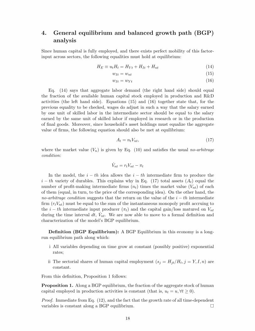
Results are summarized in Table 3 (Supporting information can be found in Ap-pendix A3).

The intuition behind the results of Proposition 3 (and Table 3) goes as follows. Byusing again the BGP equilibrium relation:

γy = γH +Rγn − gL (28)

21

0 ≤ ξ ≤ 1∂γy∂gL

> 0

1 < ξ < 1+2ΥR1+ΥR

∂γy∂gL

> 0

ξ = 1+2ΥR1+ΥR

∂γy∂gL

= 0

ξ > 1+2ΥR1+ΥR

∂γy∂gL

< 0

Table 3: The relationship between the magnitude of ξ and the sign of the effect of anincrease in the population growth rate (gL) on economic growth (γy).

One immediately observes that:

∂γy∂gL

= (∂γH∂gL

+R∂γn∂gL

)− 1

= (1

Υ

∂γn∂gL

+R∂γn∂gL

)− 1

∂γy∂gL

= (1 + ΥR

Υ)︸ ︷︷ ︸

> 0under our

assumptions

∂γn∂gL︸︷︷︸

‘ideas’ effect

− 1︸︷︷︸‘dilution’ effect

(29)

According to (29), the whole impact of population growth on real per-capita incomegrowth depends on the relative contribution of two distinct effects:

- The direct ‘dilution’ effect. This effect is always negative for the reasons that havealready been explained.

- The indirect ‘ideas’ effect. This effect describes the impact that at a certain pointin time an exogenous change of population size (due to a change of gL) may have onthe economy’s growth rate of ideas, γn (see Jones, 2003). Unlike the previous one, thiseffect is always positive, as long as 1 + θ − ξ > 0.23

So, all the rest remaining equal (in particular for given θ > 0), the smaller ξ is, themore likely it is for the indirect ‘ideas’ effect to be positive and for the first term of(29) to ultimately outweigh the negative ‘dilution’ effect, so leading to an unambiguous∂γy∂gL

> 0. This is what we observe in Table 3: when ξ ≤ 1, the ideas-effect is clearlypositive and the long-run correlation between population and economic growth rates ispositive, as well. However, when ξ starts becoming large (i.e., ξ > 1) a threshold levelof ξ (namely, ξ = (1+2ΥR)/(1+ΥR) in Table 3) does emerge such that the correlationbetween population growth and economic growth is no longer monotonous in sign alonga BGP equilibrium: it continues to be positive below the ξ-threshold, but becomesnegative above the ξ-threshold (the correlation between γy and gL vanishes when ξequals exactly the threshold). Note that if ξ is high enough the ideas-effect is negative(as 1 + θ − ξ < 0). In this case the whole impact of population growth on economicgrowth is undoubtedly negative, too (see Table 3 when ξ > (1 + 2ΥR)/(1 + ΥR)).

23The ‘ideas’ effect is given by ∂γn∂gL

. From Eq. (19), ∂γn∂gL

= Υ(1+θ−ξ)ΥR(θ−1)+θ

. Under requirements (i) and

(ii) of our Assumption, ∂γn∂gL

> 0 as long as 1 + θ − ξ > 0.

22

6. Conclusion

Three concomitant facts have motivated the present paper: 1) The inconclusivenessof the existing debate concerning the ultimate long-run effects of demographic change(population growth) on per-capita income growth); 2) The need of clarifying whether theexistence of a dilution effect of population growth can be documented empirically alsofor per-capita human capital investment (and not only for per-capita physical capitalinvestment); 3) The possibility of introducing in the ongoing discussion a new channelthrough which one can explain theoretically why the long-run correlation between pop-ulation and economic growth rates may be non-monotonous in sign, regardless of thepossible sources of population growth (i.e., fertility, mortality, migration, or ageing).In a word, this paper has tried to link the magnitude of a dilution-effect of populationgrowth on per-capita human capital formation with the theoretical explanation of thesign that the correlation between population and economic growth rates can take alonga BGP equilibrium.

In the first part of the paper we have had a thorough look at the data with theobjective of providing evidence of the presence of a dilution effect of population growthalso on per-capita human capital formation. Our empirical analysis confirms the ideathat countries experiencing high population growth tend to be more negatively effectedby population growth in terms of schooling than countries with low population growth.Furthermore, the analysis finds considerable heterogeneity of the dilution effect of pop-ulation growth on schooling across countries experiencing the same level of populationgrowth; in particular for developing economies. Such heterogeneity is likely to resultfrom the combination of various factors including different drivers of population growth(birthrates versus life expectancy), different socio-economic characteristics affecting sup-ply and demand of skilled labor, as well as differences in education policy. While futureresearch may perform contingency analyses in order to single out the moderating ef-fects of the various factors causing heterogeneity in the dilution effect of populationgrowth on human capital formation, we proceeded with investigating its consequenceson long-run economic growth. Our economic growth regression suggests that schoolingis influential and positive for long-run economic growth, and that population growth —net of schooling — is in average negatively associated with economic growth. Hence,in total, population growth may affect economic growth either positively or negatively,depending on the country-specific dilution effect on schooling.

In the second part of the paper, instead, we have taken stock of the found empiricalresults and have proposed a theoretical framework (where firms can endogenously investin technological progress — taking the form of the discovery of new ideas for newvarieties of intermediate inputs —, and agents can endogenously invest in human capitalformation) with the objective of explaining why it could realistic to come to a correlationbetween population growth and economic growth in the long-run which is undeterminedin sign. The explanation provided by our theoretical model is based on the role playedexactly by the size of the dilution effect in per-capita human capital accumulation. Moreprecisely, we show that along a BGP equilibrium the whole impact of population growthon real per-capita income growth depends on the contrast of two opposing effects. Thefirst is the already mentioned dilution-effect (of population growth on per-capita skillformation). This effect is always negative. The second is, instead, the ideas-effect.By ideas-effect we mean the effect that population growth may have on the economy’sinnovation rate. This effect is positive provided that the dilution-effect is not very large.So, depending on the size of the dilution effect, we may ultimately observe a different

23

correlation between population and economic growth rates. When the dilution effectis sufficiently low, the ideas-effect is definitely positive and prevails over the negativedilution-effect, so determining a positive long-run correlation between population andeconomic growth rates. However, when the dilution-effect starts becoming large enougha threshold-level of this effect arises such that the correlation between population growthand economic growth is no longer monotonous in sign along a BGP equilibrium: itcontinues to be positive below the dilution-effect threshold, but becomes negative aboveit. When the dilution-effect gets extremely large, then the ideas-effect becomes negativeitself, and the whole impact of population growth on economic growth is undoubtedlynegative, too. We believe that these theoretical results are consistent with the empiricalevidence discussed in the first part of the paper, and that suggests the existence ofconsiderable heterogeneity across countries as far as a dilution effect of populationgrowth on schooling is concerned. Our theory builds, hence, a bridge between such cross-country heterogeneity in the magnitude of a per-capita human capital dilution-effect ofpopulation growth and the sign of the population-economic growth rates correlationalong a BGP equilibrium.

We think that our paper leaves, in particular, an important question still open. Inour model the dilution-effect has been introduced as a parameter (greater or, at most,equal to zero) that multiplies the growth rate of population in the law of motion of per-capita human capital. For further research, it would be interesting to look into thosefactors that can make this parameter endogenous. Indeed, if countries have differentthreshold levels of the dilution-effect of population growth on the accumulation of per-capita human capital, then finding the determinants of the country-specific thresholdbecomes of fundamental importance, and may also lead us to make more accuratepolicy recommendations following the possibly different impacts of demographic changeon economic prosperity across the various regions/countries of world.

References

Acemoglu, D. (2002). Directed technical change. The Review of Economic Studies,69(4):781–809.

Barro, R. and Lee, J.-W. (2013). A new data set of educational attainment in the world,1950-2010. Journal of Development Economics, 104:184–198.

Becker, G. S. and Lewis, H. G. (1973). On the interaction between the quantity andquality of children. Journal of Political Economy, 81(2):279–288.

Benassy, J.-P. (1998). Is there always too little research in endogenous growth withexpanding product variety? European Economic Review, 42(1):61–69.

Benhabib, J. and Spiegel, M. M. (1994). The role of human capital in economic develop-ment evidence from aggregate cross-country data. Journal of Monetary Economics,34(2):143–173.

Blanchet, D. (1988). A stochastic version of the Malthusian trap model: Consequencesfor the empirical relationship between economic growth and population growth inLDC’s. Mathematical Population Studies, 1(1):79–99.

Bloom, D. E., Canning, D., and Finlay, J. E. (2010). Population aging and economicgrowth in Asia. In Ito, T. and Rose, A., editors, The Economic Consequences of De-

24

mographic Change in East Asia, volume 19 of NBER-EASE, pages 61–89. Universityof Chicago Press.

Bloom, D. E., Canning, D., and Malaney, P. N. (2000). Population dynamics andeconomic growth in Asia. Population and Development Review, 26:257–290.

Boikos, S., Bucci, A., and Stengos, T. (2013). Non-monotonicity of fertility in humancapital accumulation and economic growth. Journal of Macroeconomics, 38:44–59.

Boserup, E. (1981). Population and Technological Change: A Study of Long-TermTrends. University of Chicago Press.

Bucci, A. (2008). Population growth in a model of economic growth with human capitalaccumulation and horizontal R&D. Journal of Macroeconomics, 30(3):1124–1147.

Bucci, A. (2013). Returns to specialization, competition, population, and growth. Jour-nal of Economic Dynamics & Control, 37(10):2023–2040.

Bucci, A. (2015). Product proliferation, population, and economic growth. Journal ofHuman Capital, 9(2):170–197.

Cervellati, M. and Sunde, U. (2013). Life expectancy, schooling, and lifetime laborsupply: Theory and evidence revisited. Econometrica, 81(5):2055–2086.

Chang, T., Chu, H.-P., Deale, F. W., and Gupta, R. (2014). The relationship be-tween population growth and economic growth over 1870-2013: Evidence from abootstrapped panel-granger causality test. Technical Report 31, University of Preto-ria - Department of Economics.

Coale, A. J. and Hoover, E. M. (1958). Population Growth and Economic Developmentin Low-income Countries. Princeton University Press.

Cohen, D. and Soto, M. (2007). Growth and human capital: good data, good results.Journal of Economic Growth, 12(1):51–76.

Devereux, M. B., Head, A. C., and Lapham, B. J. (1996a). Aggregate fluctuationswith increasing returns to specialization and scale. Journal of Economic Dynamics& Control, 20(4):627–656.

Devereux, M. B., Head, A. C., and Lapham, B. J. (1996b). Monopolistic competition,increasing returns, and the effects of government spending. Journal of Money, Creditand Banking, 28(2):233–254.

Devereux, M. B., Head, A. C., and Lapham, B. J. (2000). Government spendingand welfare with returns to specialization. The Scandinavian Journal of Economics,102(4):547–561.

Dinopoulos, E. and Segerstrom, P. (1999). A Schumpeterian model of protection andrelative wages. American Economic Review, pages 450–472.

Ehrlich, P. R. (1968). The Population Bomb. New York.

Ethier, W. J. (1982). National and international returns to scale in the modern theoryof international trade. The American Economic Review, 72(3):389–405.

25

Feenstra, R. C., Inklaar, R., and Timmer, M. (2013). The next generation of the pennworld table. Technical Report 19255, NBER.

Grossman, G. M. and Helpman, E. (1993). Innovation and growth in the global economy.MIT press.

Hanushek, E. A. and Woessmann, L. (2008). The role of cognitive skills in economicdevelopment. Journal of Economic Literature 2008, 46(3):607–668.

Herzer, D., Strulik, H., and Vollmer, S. (2012). The long-run determinants of fertil-ity: one century of demographic change 1900–1999. Journal of Economic Growth,17(4):357–385.

Hsiao, C. (2003). Analysis of Panel Data. Number 34 in Econometric Society mono-graphs. Cambridge University Press.

Jones, C. I. (1995). R&D-based models of economic growth. Journal of Political Econ-omy, 103(4):759–784.

Jones, C. I. (2003). Population and ideas: A theory of endogenous growth. In Aghion,P., Frydman, R., Stiglitz, J., and Woodford, M., editors, Knowledge, Informationand Expectations in Modern Macroeconomics: In Honor of Edmund S. Phelps, pages498–521. Princeton University Press, Princeton.

Jones, C. I. (2005). Growth and ideas. In Aghion, P. and Durlauf, S., editors, Handbookof Economic Growth, chapter 16, pages 1063–1111. Elsevier-North Holland.

Kelley, A. C. (1994). The consequences of rapid population growth on human resourcedevelopment: The case of education. Technical report, Australian International De-velopment Assistance Bureau.

Kelley, A. C. and Schmidt, R. M. (1995). Aggregate population and economic growthcorrelations: the role of the components of demographic change. Demography,32(4):543–555.

Kim, G.-J. (2001). Education policies and reform in South Korea. Technical report,World Bank, Washington, D.C.

Kremer, M. (1993). Population growth and technological change: one million BC to1990. The Quarterly Journal of Economics, 108(3):681–716.

Kuznets, S. (1967). Population and economic growth. Proceedings of the AmericanPhilosophical Society, 111(3):170–193.

Li, H., Loyalka, P., Scott, R., and Wu, B. (2017). Human capital and China’s futuregrowth. Journal of Economic Perspectives, 31(1):25–48.

Li, H. and Zhang, J. (2007). Do high birth rates hamper economic growth? The Reviewof Economics and Statistics, 89(1):110–117.

Liu, C., Zhang, L., Luo, R., Rozelle, S., Sharbono, B., and Shi, Y. (2009). Developmentchallenges, tuition barriers, and high school education in China. Asia Pacific Journalof Education, 29(4):503–520.

26

Lucas, R. E. (1988). On the mechanics of economic development. Journal of MonetaryEconomics, 22(1):3–42.

Mierau, J. O. and Turnovsky, S. J. (2014). Demography, growth, and inequality. Eco-nomic Theory, 55(1):29–68.

Montgomery, M. R., Arends-Kuenning, M., and Mete, C. (2000). The quantity-qualitytransition in Asia. Population and Development Review, 26:223–256.

Prettner, K. (2014). The non-monotonous impact of population growth on economicprosperity. Economics Letters, 124(1):93–95.

Romer, P. M. (1986). Increasing returns and long-run growth. Journal of PoliticalEconomy, 94(5):1002–1037.

Romer, P. M. (1987). Growth based on increasing returns due to specialization. TheAmerican Economic Review, 77(2):56–62.

Romer, P. M. (1990). Endogenous technological change. Journal of Political Economy,98(5, Part 2):S71–S102.

Simon, J. (1981). The Ultimate Resource. Princeton: Princeton University Press.

Solow, R. M. (1956). A contribution to the theory of economic growth. The QuarterlyJournal of Economics, 70(1):65–94.

Strulik, H. (2005). The role of human capital and population growth in R&D-basedmodels of economic growth. Review of International Economics, 13(1):129–145.

United Nations (2015). World Population Prospects: The 2015 Revision, DVD Edition.United Nations, Department of Economic and Social Affairs, Population Division.

Uzawa, H. (1965). Optimum technical change in an aggregative model of economicgrowth. International Economic Review, 6(1):18–31.

27

A Appendix

A1 Data

This subsection provides averages of the main variables used in the empirical sectionby region: i) ‘Avg. years of schooling’ (i.e. average years of schooling in the populationof the 15 to 100 years old), ii) ‘Years of schooling young cohort’ (i.e. schooling of thethen 5 to 9 years old cohort, attained until age 25 to 29 years), iii) ‘GDP p. adult’ (i.e.output-side real GDP at chained PPPs (in thousand 2005 US$) per person above 20years, iv) ‘GDP p. capita’ (i.e. output-side real GDP at chained PPPs (in thousand2005 US$) per person), v) ‘Population growth rate’ (i.e. natural population growthrate, crude birth rate minus crude death rate, per 100 population). All variables inlogs. Five African countries (Botswana, Mali, Mozambique, Niger, Senegal) are outliersin terms of schooling advancement, and hence removed from the working sample.

Table 4: Advanced Economies1

Year Avg. years of Years of schooling GDP p. adult GDP p. capita Populationschooling in logs young cohort in logs in logs in logs growth rate

1960 1.97 (0.28) 2.41 (0.16) 2.59 (0.62) 2.14 (0.67) 1.09 (0.45)1965 2.02 (0.27) 2.47 (0.13) 2.84 (0.49) 2.38 (0.53) 0.89 (0.4)1970 2.1 (0.25) 2.51 (0.11) 3.03 (0.41) 2.6 (0.43) 0.74 (0.49)1975 2.18 (0.22) 2.53 (0.1) 3.15 (0.4) 2.74 (0.41) 0.6 (0.5)1980 2.25 (0.2) 2.55 (0.07) 3.32 (0.29) 2.93 (0.31) 0.52 (0.46)1985 2.29 (0.17) 2.58 (0.06) 3.3 (0.3) 2.95 (0.32) 0.47 (0.42)1990 2.33 (0.15) 2.6 (0.07) 3.49 (0.26) 3.16 (0.28) 0.45 (0.39)1995 2.37 (0.12) — 3.59 (0.25) 3.28 (0.27) 0.37 (0.36)2000 2.41 (0.1) — 3.79 (0.26) 3.49 (0.26) 0.34 (0.36)2005 2.45 (0.11) — 3.85 (0.3) 3.57 (0.29) 0.37 (0.37)2010 2.49 (0.11) — 3.9 (0.29) 3.63 (0.28) 0.31 (0.4)

1 25 countries: Australia, Austria, Belgium, Canada, Cyprus, Denmark, Finland, France, Greece, Iceland,Ireland, Israel, Italy, Japan, Luxembourg, Malta, Netherlands, New Zealand, Norway, Portugal, Spain,Sweden, Switzerland, United Kingdom, USA.

28

Table 5: Asia1

Year Avg. years of Years of schooling GDP p. adult GDP p. capita Populationschooling in logs young cohort in logs in logs in logs growth rate

1960 1.21 (0.48) 1.8 (0.49) 1.23 (0.55) 0.51 (0.53) 2.65 (0.47)1965 1.32 (0.49) 1.95 (0.45) 1.37 (0.59) 0.62 (0.57) 2.5 (0.44)1970 1.46 (0.5) 2.02 (0.43) 1.58 (0.68) 0.83 (0.69) 2.35 (0.4)1975 1.56 (0.49) 2.14 (0.39) 1.73 (0.79) 1.01 (0.82) 2.18 (0.59)1980 1.67 (0.47) 2.2 (0.4) 1.84 (0.89) 1.17 (0.96) 2.11 (0.64)1985 1.78 (0.42) 2.31 (0.32) 1.88 (0.84) 1.25 (0.94) 1.98 (0.69)1990 1.88 (0.39) 2.38 (0.29) 2.07 (0.91) 1.48 (1.02) 1.8 (0.67)1995 1.98 (0.38) — 2.23 (0.88) 1.68 (1) 1.55 (0.75)2000 2.05 (0.35) — 2.26 (0.96) 1.74 (1.08) 1.36 (0.7)2005 2.14 (0.3) — 2.4 (1.03) 1.93 (1.16) 1.21 (0.63)2010 2.21 (0.28) — 2.66 (0.89) 2.22 (1.02) 1.09 (0.58)

1 14 countries: Bangladesh, China, China, Hong Kong Special Administrative Region, Fiji, India, Indonesia,Malaysia, Nepal, Pakistan, Philippines, Republic of Korea, Singapore, Sri Lanka, Thailand.

Table 6: Latin America and the Caribbean1

Year Avg. years of Years of schooling GDP p. adult GDP p. capita Populationschooling in logs young cohort in logs in logs in logs growth rate

1960 1.41 (0.34) 1.91 (0.29) 1.91 (0.63) 1.17 (0.65) 2.81 (0.67)1965 1.5 (0.34) 2.04 (0.27) 2.05 (0.66) 1.28 (0.67) 2.65 (0.69)1970 1.6 (0.34) 2.1 (0.24) 2.19 (0.71) 1.42 (0.72) 2.5 (0.68)1975 1.69 (0.32) 2.19 (0.19) 2.3 (0.68) 1.55 (0.7) 2.43 (0.67)1980 1.8 (0.28) 2.23 (0.19) 2.34 (0.66) 1.63 (0.69) 2.35 (0.68)1985 1.9 (0.25) 2.29 (0.19) 2.22 (0.61) 1.54 (0.66) 2.19 (0.65)1990 1.97 (0.23) 2.33 (0.19) 2.23 (0.61) 1.58 (0.68) 2 (0.64)1995 2.04 (0.22) — 2.36 (0.58) 1.75 (0.67) 1.79 (0.63)2000 2.1 (0.2) — 2.43 (0.54) 1.85 (0.64) 1.58 (0.57)2005 2.16 (0.2) — 2.55 (0.53) 2.02 (0.62) 1.41 (0.52)2010 2.2 (0.18) — 2.73 (0.57) 2.24 (0.64) 1.26 (0.48)

1 22 countries: Argentina, Barbados, Bolivia, Brazil, Chile, Colombia, Costa Rica, Dominican Rep.,Ecuador, El Salvador, Guatemala, Haiti, Honduras, Jamaica, Mexico, Nicaragua, Panama, Paraguay, Peru,Trinidad and Tobago, Uruguay, Venezuela.

29

Table 7: Middle East and North Africa1

Year Avg. years of Years of schooling GDP p. adult GDP p. capita Populationschooling in logs young cohort in logs in logs in logs growth rate

1960 0.75 (0.26) 1.63 (0.22) 1.69 (0.84) 0.94 (0.82) 2.95 (0.51)1965 0.89 (0.26) 1.81 (0.21) 1.87 (0.67) 1.08 (0.66) 2.95 (0.54)1970 1.05 (0.25) 1.96 (0.21) 2.04 (0.68) 1.22 (0.67) 2.95 (0.57)1975 1.23 (0.23) 2.02 (0.17) 2.22 (0.74) 1.41 (0.72) 2.98 (0.49)1980 1.41 (0.21) 2.11 (0.19) 2.13 (0.68) 1.33 (0.66) 2.94 (0.45)1985 1.6 (0.2) 2.2 (0.18) 2.19 (0.66) 1.41 (0.67) 2.66 (0.47)1990 1.73 (0.19) 2.27 (0.19) 2.15 (0.63) 1.39 (0.68) 2.24 (0.47)1995 1.83 (0.2) — 2.22 (0.64) 1.52 (0.71) 1.91 (0.57)2000 1.92 (0.21) — 2.34 (0.55) 1.71 (0.62) 1.71 (0.57)2005 2.01 (0.19) — 2.6 (0.38) 2.04 (0.43) 1.7 (0.5)2010 2.1 (0.17) — 2.84 (0.34) 2.34 (0.39) 1.72 (0.48)

1 8 countries: Algeria, Egypt, Iran, Jordan, Morocco, Syrian Arab Republic, Tunisia, Turkey.

Table 8: Sub-Saharan Africa1

Year Avg. years of Years of schooling GDP p. adult GDP p. capita Populationschooling in logs young cohort in logs in logs in logs growth rate

1960 0.85 (0.37) 1.47 (0.42) 1.21 (0.57) 0.46 (0.59) 2.57 (0.59)1965 0.95 (0.37) 1.64 (0.37) 1.35 (0.61) 0.58 (0.64) 2.7 (0.47)1970 1.07 (0.38) 1.76 (0.37) 1.49 (0.59) 0.7 (0.63) 2.84 (0.46)1975 1.21 (0.36) 1.84 (0.35) 1.57 (0.63) 0.77 (0.67) 2.98 (0.43)1980 1.35 (0.34) 1.89 (0.29) 1.58 (0.67) 0.78 (0.71) 3 (0.48)1985 1.46 (0.33) 1.93 (0.27) 1.62 (0.64) 0.81 (0.68) 2.92 (0.44)1990 1.58 (0.33) 1.99 (0.26) 1.52 (0.71) 0.71 (0.77) 2.59 (0.7)1995 1.68 (0.31) — 1.43 (0.78) 0.63 (0.85) 2.49 (0.53)2000 1.74 (0.28) — 1.44 (0.78) 0.66 (0.87) 2.38 (0.72)2005 1.83 (0.26) — 1.53 (0.8) 0.77 (0.89) 2.47 (0.8)2010 1.89 (0.25) — 1.63 (0.8) 0.88 (0.88) 2.5 (0.76)

1 23 countries: Benin, Burundi, Cameroon, Central African Republic, Congo, Cote d’Ivoire, DemocraticRepublic of the Congo, Gabon, Gambia, Ghana, Kenya, Lesotho, Malawi, Mauritania, Mauritius, Namibia,Rwanda, South Africa, Togo, Uganda, United Republic of Tanzania, Zambia, Zimbabwe.

30

A2 Eqs. (18) and (27)

The Hamiltonian function (Jt) related to the intertemporal problem (13) in the main-text is:

Jt = (c1−θt − 1

1− θ)e−(ρ−gL)t + λat[(rt − gL)at + (utht)wt − ct] + λht[σ(1− ut)− ξgL]ht

where λat and λht are the co-state variables associated, respectively, to the statevariables at and ht.The necessary first order conditions FOC s are:

∂Jt∂ct

= 0⇐⇒ e−(ρ−gL)t

cθt= λat (A1)

∂Jt∂ut

= 0⇐⇒ λat =σ

wtλht (A2)

∂Jt∂at

= − ˙λat ⇐⇒ λat(rt − gL) = − ˙λat (A3)

∂Jt∂ht

= − ˙λht ⇐⇒ λatutwt + λht[σ(1− ut)− ξgL] = − ˙λht (A4)

along with the two transversality conditions:

limt→∞

λatat = 0, limt→∞

λhtht = 0

and the initial conditions:

a(0) > 0, h(0) > 0

Combining (A2) and (A4) yields:

˙λhtλht

= −(σ − ξgL) (A5)

Eqs. (A3) and (A2) imply, respectively:

˙λatλat

= −(rt − gL) (A6)

˙λatλat

=˙λhtλht− wtwt

(A7)

Combination of (A5), (A6) and (A7) leads to:

rt = (1− ξ)gL + σ +wtwt

(A8)

Since human capital is perfectly mobile across sectors, at equilibrium it will be rewardedaccording to the same wage: wt ≡ wY t = wIt = wnt. Moreover, along the BGP thiscommon wage would grow at a constant exponential rate, implying that γw is constant.Accordingly, in the BGP equilibrium the real rate of return on asset holdings, r, will beconstant (Eq. A8). With r constant, and making use of Eqs. (6) and (10) in the maintext, we find that along the BGP:

Vnt = Z(1− Z)(HY t

nt)1−Z(

HIt

nt)Z

nRt[r + (1−R)γn − γH ]

, (A9)

R ≡ α+ 1− Z, ntnt≡ γn,

Ht

Ht≡ γH

31

For any 0 < Z < 1, HY > 0, HI > 0, n > 0 and R > 0, Vnt is positive provided that:

r > γH − (1−R)γn (A9′)

Given Vnt , from Eq. (9′) in the main text:

wnt =Z

χ(1− Z)sµ−1

n Hµ−1−Φt nηt (

HY t

nt)1−Z(

HIt

nt)Z

nRt[r + (1−R)γn − γH ]

(A10)

where sn ≡ Hnt/Ht is constant along the BGP. We can now use Eqs. (5), (2) and (4′)in the main text, obtaining:

wIt = Z2(HY t

nt)1−Z(

HIt

nt)Z−1nRt (A11)

From Eq. (15) in the main text, by equalizing (A11) and (A10) in this appendix, onegets:

sI ≡HIt

Ht=

Zχ

(1− Z)

[r + (1−R)γn − γH ]

sµ−1n

n1−ηt

Hµ−Φt

(A12)

Combining Eqs. (1) and (4′) in the text:

wY t ≡∂Yt∂HY t

= (1− Z)(HY t

nt)−Z(

HIt

nt)ZnRt (A13)

From (16) in the main text and (A12) above, equalization of Eqs. (A11) and (A13) inthis appendix delivers:

sY ≡HY t

Ht= (

1− ZZ2

)sI =χ

Z

[r + (1−R)γn − γH ]

sµ−1n

n1−ηt

Hµ−Φt

(A14)

Along the BGP all variables depending on time grow at constant rates and the sectorshares of human capital employment are also constant. Therefore, from Eq. (8) in themain text:

ntnt≡ γn = (

µ− Φ

1− η)γH , γH ≡

Ht

Ht(A15)

If µ−Φ = 1−η we have a very special case of the model in which human and technologicalcapital grow at the same rate γn = γH ≡ γ along a BGP. We rule out this “extreme”case and analyze the most general possible situation in which: µ 6= Φ 6= Φ + 1− η.

Using Eqs. (A10), (A11), (A13) and (A15) we see that along the BGP wages growat a common and constant rate:

˙wntwnt

=wItwIt

=˙wY t

wY t≡ wtwt

= Rγn (A15′)

Combining Eqs. (A1) and (A6), the usual Euler equation follows:

ctct≡ 1

θ(r − ρ), c ≡ C

L(A16′)

From (17) in the text and (A9) in this appendix we conclude that along a BGP:

atat≡ γa = γH +Rγn − gL, at ≡

AtLt, gL ≡

LtLt

(A17)

32

Merging (11′) in the main text and (A6) in this appendix yields:

˙λatλat

= −γa + uthtwtat− ctat, (A18)

where ut = u,∀t ≥ 0 along the BGP. Instead, from the combination of (12) in the textand (A5) in this appendix we get:

˙λhtλht

= −λh − σµ, ht ≡Ht

Lt, γh ≡

htht

(A19)

Eqs. (A7), (A15′), (A17), (A18) and (A19) together lead to:

ctat

= u[htwtat

+ σ], (A20)

where γh = γH − gL has been used.Using (12) in the main text, Eqs. (A15′), (A17) and (A20) and the fact that γH =

γh + gL = σ(1− u) + (1− ξ)gL one obtains:

ctat

= u[h(0)w(0)

a(0)+ σ] (A20′)

where h(0), w(0) and a(0) are the initial values (i.e., at t = 0) of ht, wt and at, re-spectively. With u constant, the just-mentioned initial values given, and σ > 0 the lastequation implies:

γc = γa (A21)

This means that along the BGP at and ct grow at the same rate. Using (A21) andequating (A16′) and (A17) it is possible to get:

r = ρ+ θ(γH +Rγn − gL) (A22)

Next, by equalizing (A22) to (A8), and using (A15′):

γn ≡ntnt

=[(σ − ρ)− (ξ − 1− θ)gL − θγH ]

R(θ − 1)(A23)

Equating (A23) to (A15), and solving for γH , we finally obtain:

γH ≡Ht

Ht=

[(σ − ρ)− (ξ − 1− θ)gL]

ΥR(θ − 1) + θ, Υ ≡ [

µ− Φ

1− η] (A23′)

Given γH , it is possible to re-cast γn as:

γn ≡ntnt

=Υ[(σ − ρ)− (ξ − 1− θ)gL]

ΥR(θ − 1) + θ= ΥγH (A23′′)

Eqs. (A23′) and (A23′′) confirm that

γH = γn

33

in the special case in which Υ ≡ µ−Φ1−η = 1. The BGP equilibrium - value of r is obtained

by combining (A22), (A23′) and (A23′′):

r =σθ + ΥR(σθ − ρ)− θ[ξ(1 + ΥR)− (1 + 2ΥR)]gL

ΥR(θ − 1) + θ(A22′)

Eqs. (A21) and (A16′) together imply:

γa ≡atat

= γc ≡ctct

=1

θ(r − ρ) where r is given by Eq. (A22′) (A21′)

After using Eq. (12) in the main text, the definition of h ≡ H/L and the fact thatL/L ≡ gL, we conclude:

γH ≡H

H= σ(1− u) + (1− ξ)gL (A24)

Equalization of (A23′) and (A24) allows obtaining the BGP equilibrium value of u:

u = 1− (σ − ρ)− [ΥR(1− ξ)(θ − 1) + ξ(1− θ)− 1]gLσ[ΥR(θ − 1) + θ]

(A25)

From (1) in the text, (A22′), (A23′) and (A23′′) in this appendix, the hypothesis ofsymmetry (Eq. 4′ in the text), the definitions of y ≡ Y/L, R ≡ α+1−Z and L/L ≡ gL,we obtain the growth rate of real per-capita output along a BGP:

γy ≡ytyt

=(1 + ΥR)(σ − ρ)− [ΥR(ξ − 2) + (ξ − 1)]gL

ΥR(θ − 1) + θ= γa = γc =

1

θ(r − ρ) (A26)

We now compute the BGP equilibrium values of sn, sI and sY . Eq. (14) in the main

text suggests: u = sY + sI + sn From (A14) in this appendix we use sy = (1− ZZ2

)sI

into the expression above and obtain:

sI = [Z2

1− Z + Z2](u− sn) where u is given by A25. (A27)

Hence:

sY = [1− Z

1− Z + Z2](u− sn) (A28)

According to (A14), however, it is also true that:

sY ≡HY t

Ht=χ

Z

[r + (1−R)γn − γH ]

sµ−1n

n1−ηt

Hµ−Φt

Equating this expression to (A28) yields:

Hµ−Φt

n1−ηt

=χ[1− Z + Z2]

Z(1− Z)

[r + (1−R)γn − γH ]

sµ−1n (u− sn)

(A29)

From Eq. (8) in the body-text:

Hµ−Φt

n1−η =χ

sµnγn (A30)

34

Equalization of (A29) and (A30) leads to:

sn =Z(1− Z)γn

[1− Z + Z2][r + (1−R)γn − γH ] + Z(1− Z)γnu (A31)

Given Eqs. (A22′), (A23′), (A23′′), (A25) and (A31), it is possible to compute the BGP

ratioHµ−Φtn1−η (by using either Eq. 29 or Eq. A30), along with sI and sY (Eqs. A27 and

A28).Finally, by employing Eqs. (A6), (A7), (A15′), (A17) and the definition of h, it

can be showed that along a BGP the two transversality conditions limt→∞ λatat = 0and limt→∞ λhtht = 0 are simultaneously checked when: r > γH + Rγn. In turn,when the two transversality conditions are met, then the requirement (Eq. A9′): r >γH − (1−R)γn is also met.

A3 Table 3

∂γy∂gL

=−[ΥR(ξ − 2) + (ξ − 1)]

ΥR(θ − 1) + θ

When assumptions (i) and (ii) in the main text are met, [ΥR(θ − 1) + θ] is alwayspositive. With Υ > 0, R > 0, and ξ ≥ 0 we conclude:

• ∂γy∂gL

> 0⇒

−ΥR(ξ − 2)− (ξ − 1) > 0

−ΥR(ξ − 2) > (ξ − 1)

ΥRξ + ξ < 1 + 2ΥR

ξ(1 + ΥR) < 1 + 2ΥR

0 < ξ <1 + 2ΥR

1 + ΥR

• ∂γy∂γL

< 0⇒ −ΥR(ξ − 2)− (ξ − 1) < 0 ⇒ ξ > 1+2ΥR1+ΥR

• ∂γy∂gL

= 0⇒ −ΥR(ξ − 2)− (ξ − 1) = 0 ⇒ ξ = 1+2ΥR1+ΥR

• if ξ = 1⇒ ∂γy∂gL

= −[ΥR(−1)]ΥR(θ−1)+θ = ΥR

ΥR(θ−1)+θ ⇒ ∂γy∂gL

> 0

• if ξ = 0⇒ ∂γy∂gL

= −[ΥR(−2)+(−1)]ΥR(θ−1)+θ) = 2ΥR+1

ΥR(θ−1)+θ ⇒∂γy∂gL

> 0

35

No. 113

No. 112

No. 111

No. 110

No. 109

No. 108

No. 107

No. 106

No. 105

No. 104

No. 103

Alberto Bucci, Levent Eraydın, Moritz Müller: Dilution effects, population

growth and economic growth under human capital accumulation and

endogenous technological change, January 2018

Jochen Schweikert and Markus Höchstötter: Epidemiological spreading

of mortgage default, January 2018

Armin Falk and Nora Szech: Diffusion of being pivotal and immoral out-

comes, December 2017

Leonie Kühl and Nora Szech: Physical distance and cooperativeness to-

wards strangers, November 2017

Deniz Dizdar, Benny Moldovanu and Nora Szech: The multiplier effect in

two-sided markets with bilateral investments, November 2017

Andranik S. Tangian: Policy representation by the 2017 Bundestag, Sep-

tember 2017

Andranik S. Tangian: Policy representation by German parties at the 2017

federal election, September 2017

Andranik S. Tangian: Design and results of the third vote experiment

during the 2017 election of the Karlsruhe Institute of Technology student

parliament , September 2017

Markus Fels: Incentivizing efficient utilization without reducing access:

The case against cost-sharing in insurance, July 2017

Andranik S. Tangian: Declining labor–labor exchange rates as a cause of

inequality growth, July 2017

Konstanze Albrecht, Florentin Krämer and Nora Szech: Animal welfare

and human ethics: A personality study, June 2017

recent issues

Working Paper Series in Economics

The responsibility for the contents of the working papers rests with the author, not the Institute. Since working papers

are of a preliminary nature, it may be useful to contact the author of a particular working paper about results or ca-

veats before referring to, or quoting, a paper. Any comments on working papers should be sent directly to the author.