dilation theorems for vh-spaces · abstract dilation theorems for vh-spaces bar ˘s evren u gurcan...

DILATION THEOREMS FOR VH-SPACES

a thesis

submitted to the department of mathematics

and the institute of engineering and science

of bilkent university

in partial fulfillment of the requirements

for the degree of

master of science

By

Barıs Evren Ugurcan

June, 2009

I certify that I have read this thesis and that in my opinion it is fully adequate,

in scope and in quality, as a thesis for the degree of Master of Science.

Assoc. Prof. Aurelian Gheondea (Supervisor)



Prof. Dr. Mefharet Kocatepe



Prof. Dr. Cihan Orhan

Approved for the Institute of Engineering and Science:

Prof. Dr. Mehmet B. BarayDirector of the Institute Engineering and Science

ii

ABSTRACT

DILATION THEOREMS FOR VH-SPACES


M.S. in Mathematics

Supervisor: Assoc. Prof. Aurelian Gheondea

June, 2009

In the Appendix of the book Lecons d’analyse fonctionnelle by F. Riesz and

B. Sz.-Nagy, B. Sz.-Nagy [15] proved an important theorem on operator valued

positive definite maps on ∗-semigroups, which today can be considered as one of

the pioneering results of dilation theory. In the same year W.F. Stinespring [11]

proved another celebrated theorem about dilation of operator valued completely

positive linear maps on C∗-algebras. Then F.H. Szafraniec [14] showed that these

theorems are actually equivalent.

Due to reasons coming from multivariate stochastic processes R.M. Loynes [7],

considered a generalization of B. Sz.-Nagy’s Theorem for vector Hilbert spaces

(that he called VH-spaces). These VH-spaces have “inner products” that are

vector valued, into the so-called “admissible spaces”.

This work is aimed at providing a detailed proof of R.M. Loynes Theorem that

generalizes B. Sz.-Nagy, a detailed proof of the equivalence of Stinespring’s The-

orem in the Arveson formulation [2] for B∗-algebras with B. Sz.-Nagy’s Theorem

following the lines in [14] together with some ideas from [2], and to get VH-

variants of Stinespring’s Theorem for C∗-algebras and B∗-algebras. Relations

between these theorems are also considered.

Keywords: C∗-Algebras , VH-Spaces, Completely positive maps, Dilation .

iii

OZET

VH-UZAYLARINDA GENLESME TEOREMLERI


Matematik, Yuksek Lisans

Tez Yoneticisi: Doc. Dr. Aurelian Gheondea

Haziran, 2009

F. Riesz ve Sz.-Nagy tarafından yazılmıs olan Lecons d’analyse fonctionnelle

adlı kitabın ek bolumunde, Sz.Nagy [15] bugun genlesme teorisinin en onemli

sonuclarından biri sayılan ∗-semigruplar uzerinde pozitif tanımlı operator degerli

fonksiyonlarla ilgili bir teorem ispatladı. Aynı yıl W.F. Stinespring [11] de C∗-

cebirleri uzerinde tamamen pozitif fonksiyonlar icin baska bir teorem ispatladı.

Daha sonra F.H. Szafraniec [14] bu iki teoremin aslında esdeger oldugunu gosterdi.

R.M. Loynes, motivasyonunu cok degiskenli stokastik modellerden aldıgı

uzerinde, degerini uygun secilmis bir topolojik uzayda alan, vektor degerli bir

ic carpım tanımlı olan VH-uzaylarını tanımlayarak B. Sz.-Nagy nin teoreminin

bir versiyonunu bu uzaylar icin ispatladı.

Bu tezin amacı ; R.M. Loynes’in yukarıda bahsedilen teoreminin ayıntılı bir

ispatını verip, bu teoremin ve Steinspring teoreminin Arveson tarafından B∗-

cebirleri icin ispatlanan [2] versiyonunun [14] u takip ederek ve [2] den fikirler

kullanarak esdeger olduklarını gosterip, Steinspring teoreminin C∗ ve B∗-cebirleri

icin VH-uzaylarında benzerlerini elde ederek bu teoremlerin R.M. Loynes’in teo-

remiyle olan iliskilerini incelemektir.

Anahtar sozcukler : C∗-Cebirleri, VH-Uzay, Tamamen pozitif operatorler, Stine-

spring temsili .

iv

Acknowledgement

I would like to express my deepest gratitude to my advisor Prof. Aurelian

Gheondea for his great guidance, instructive comments and valuable suggestions.

I would like to thank him for providing such a productive and dynamic envi-

ronment especially through the weekly meetings. I would like to mention that I

enjoyed a lot working on the topics we have chosen and learned many important

things which I will use throughout my career. I am glad to have the chance to

work with him.

I would like to thank professors Iossif V. Ostrovskii, Azer Kerimov, Hakkı

Turgay Kaptanoglu, Mefharet Kocatepe and all of other department members

who I think made possible the friendly and prolific atmosphere in our department.

I would like to mention that I have always been happy being a member of this

department.

I would like to thank Prof. Mefharet Kocatepe and Prof. Cihan Orhan for

accepting to read and review my thesis.

The work which form the content of this thesis is financially supported by

TUBITAK through the post-graduate fellowship program, namely ”TUBITAK-

BIDEB 2210-Yurt Ici Yuksek Lisans Burs Programı”. I would like to thank the

Council for their kind support.

I would like to thank my family for their constant encouragement and support

in all stages of my life. Especially, for putting their trust in me since my childhood.

v

Contents

1 Introduction 1

2 Preliminaries on C∗ and B∗-Algebras 3

3 VH-spaces 7

3.1 Definitions and Basic Theorems . . . . . . . . . . . . . . . . . . . 7

3.2 Linear Operators on VH-Spaces . . . . . . . . . . . . . . . . . . . 12

3.3 Self-Adjoint Operators in B∗(H) . . . . . . . . . . . . . . . . . . . 17

3.4 Accessible Subspaces and Projections . . . . . . . . . . . . . . . . 17

4 Dilations of B∗(H) Valued Maps 19

5 Stinespring and Sz.-Nagy Theorems 29

6 Dilation Theorems for VH-Spaces 35

6.1 Stinespring’s Theorem for VH-Spaces . . . . . . . . . . . . . . . . 35

6.2 A Comparison of Dilation Theorems for VH-Spaces . . . . . . . . 40

1

Dilation Theorems for VH-Spaces


June 22, 2009

Chapter 1

Introduction

In the Appendix of the book Lecons d’analyse fonctionnelle by F. Riesz and

B. Sz.-Nagy, B. Sz.-Nagy [15] proved an important theorem on operator valued

positive definite maps on ∗-semigroups, which today can be considered as one of

the pioneering results of dilation theory. In the same year W.F. Stinespring [11]

proved another celebrated theorem on dilations of operator valued completely

positive linear maps on C∗-algebras. Then F.H. Szafraniec [14] showed that these

theorems are actually equivalent.

Due to reasons coming from multivariate stochastic processes, R.M. Loynes [7],

considered a generalization of B. Sz.-Nagy’s Theorem for vector Hilbert spaces

(that he called VH-spaces). These VH-spaces have “inner products” that are

vector valued, into the so-called “admissible spaces”. There are of course reasons

why studying such objects turns out to be important. Let A be a commutative

C∗-algebra. By the important theorem of Gelfand-Naimark we know that A can

be identified with the continuous functions C(X) on a locally compact Hausdorff

space X. When X is a Euclidean manifold it is natural to consider the tangent

spaces at each point to study the manifold. However, this is more a geometric

point of view. The important shift of approach might be considering a Hilbert

space at each point of the manifold. If we are to express this in a technical way

we can take a Hilbert space Ht at each t ∈ X. In any of these Hilbert spaces

there is an inner product. In fact, all of these Hilbert spaces are glued together

1

CHAPTER 1. INTRODUCTION 2

so as to form a vector bundle E. In this vector bundle we can define the inner

product of two sections, say ξ and η, 〈ξ, η〉 as following function

t 7−→ 〈ξ(t), η(t)〉.

As seen, with this definition the vector bundle E is now equipped with a

C(X)-valued inner product. This is an important example from [6] which shows

why the spaces having inner product in a more general space might be important.

One of the most important such objects are Hilbert C∗-modules in which case

the inner product takes its values in a C∗-algebra. However, when one examines

the proofs of several dilation theorems it might be seen that the techniques can

even generalize to more general spaces than the Hilbert C∗-modules. The spaces

we will examine in this thesis are VH-spaces. In the case of VH-spaces the

inner product takes its values in a suitable topological vector space. The most

important point is that VH-spaces lack the multiplicative structure, after all it is

just a vector space. As we will see, yet this weak-structured spaces enjoy many

useful properties of the usual Hilbert spaces. Some of the difficulties here are the

lack of Riesz Representation Theorem [7] and the Schwarz inequality. In fact,

it is not possible to expect a kind of Schwarz inequality since, as we mentioned,

the inner product takes its values in a topological space lacking a multiplicative

structure. However, many of the theorems and techniques can be adapted to this

case, too.

This work is aimed at providing a detailed proof of R.M. Loynes Theorem that

generalizes B. Sz.-Nagy, a detailed proof of the equivalence of Stinespring’s The-

orem in the Arveson formulation [2] for B∗-algebras, with B. Sz.-Nagy’s Theorem

following the lines in [14] together with some ideas from [2], and to get VH-

variants of Stinespring’s Theorem for C∗-algebras and B∗-algebras. Relations

between these theorems are also considered.

Chapter 2

Preliminaries on C∗ and

B∗-Algebras

In this chapter we recall a few definitions and facts from the theory of operator

algebras that we will use. We assume known all basic notions in Hilbert spaces

and operators on Hilbert spaces, e.g. see [4].

Definition 2.1. By an algebra over C we mean a complex vector space A to-

gether with a binary operation representing multiplication A 3 x, y 7→ xy ∈ Asatisfying

1. Bilinearity: For α, β ∈ C and x, y, z ∈ A we have

(αx+ βy)z = α · xz + β · yz,

x(α · y + β · z) = α · xy + β · xz.

2. Associativity: x(yz) = (xy)z.

Definition 2.2. A normed algebra is a pair (A, ‖ · ‖) consisting of an algebra

together with a norm ‖ · ‖ : A 7→ [0,∞) which is related to the multiplication as

3

CHAPTER 2. PRELIMINARIES ON C∗ AND B∗-ALGEBRAS 4

follows:

‖xy‖ ≤ ‖x‖‖y‖, x, y ∈ A.

A Banach algebra is a normed algebra that is a (complete) Banach space

relative to its given norm.

Definition 2.3. If A is a Banach algebra, an involution is a map a 7→ a∗ of A

into itself such that for all a and b in A all scalars α the following hold:

1. (a∗)∗ = a

2. (ab)∗ = b∗a∗

3. (αa+ b)∗ = αa∗ + b∗

Additionally, an algebra which has an identity is called unital.

Definition 2.4. A C∗-algebra is a Banach algebra with involution such that

‖a∗a‖ = ‖a‖2

for every a in A.

Definition 2.5. For every element x in a unital C∗-algebra A, the spectrum of

x is defined as the set

σ(x) = λ ∈ C : x− λ 6∈ A−1

where A−1 denotes the set of all invertible elements in A.

Definition 2.6. If A is a C∗-algebra and a ∈ A, then:

• a is hermitian if a = a∗

• a is normal if a∗a = aa∗.

• when A is unital, a is unitary if a∗a = aa∗ = 1


For any C∗-algebra A, Ah will denote the collection of hermitian elements of

A.

Definition 2.7. If A is a C∗-algebra, an element a of A is positive if a ∈ Ah and

σ(a) ⊆ R+, the set of non-negative real numbers. This property is denoted by

a ≥ 0 and A+ denotes the collection of all positive elements in A. We say that an

element is negative if −a ∈ A+. We can write this as a ≤ 0 and A− the collection

of all negative elements in A.

Theorem 2.8. If A is a C∗-algebra the following statements are equivalent

1. a ≥ 0

2. a = b2 for some b in A+

3. a = x∗x for some x in A.

The set of all bounded operators on a Hilbert space is denoted by B(H). In

fact, the following proposition gives an important property of positive operators

on the Hilbert space H.

Proposition 2.9. If H is a Hilbert space and A ∈ B(H), then A is positive if

and only if 〈Ah, h〉 ≥ 0 for every vector h.

Definition 2.10. A map ϕ : A → B(H), where A is a ∗-algebra, is said to be

positive definite (shortly PD) if

∑i,j

(ϕ(s∗jsi)fi, fj) ≥ 0

for any finite number of s1, s2, . . . , sn in A and f1, f2, . . . , fn in H. A linear map

µ : A→ B(H), where A is a C∗-algebra, is said to be completely positive (shortly

CP) if for each n, µ(n) is a positive map of An into B(Hn) where An is the C∗-

algebra of all matrices (aij) with entries aij in A and µn((aij)) = (µ(aij)). Since for

any positive square matrix (aij) in An can be written as linear combination (with

positive coefficients) of matrices of type (b∗jbi), for a linear map on C∗-algebra

positive definiteness and complete positivity coincide.


Definition 2.11. A Banach ∗-algebra (or B∗-algebra) is a Banach algebra A that

is endowed with an involution x 7→ x∗ satisfying ‖x∗‖ = ‖x‖, x ∈ A.

Definition 2.12. A representation of a Banach ∗-algebra is a homomorphism

π : A → B(H) of A into the ∗-algebra of bounded operators on some Hilbert

space satisfying π(x∗) = π(x)∗ for all x ∈ A.

Proposition 2.13. Let A be a B∗-algebra with unit. Let R be the set of repre-

sentations of A. For each x ∈ A, we define

‖x‖′ = supπ∈R‖π(x)‖.

We have that ‖x‖′ ≤ ‖x‖. Also, the map x 7→ ‖x‖′ is a semi-norm on A which

satisfies

• ‖xy‖′ ≤ ‖x‖′‖y‖′

• ‖x∗‖′ = ‖x‖′

• ‖x∗x‖′ = ‖x‖′2

With the notation as in the previous proposition, let I be the set of x ∈ Asuch that ‖x‖′ = 0. Observe that I is a closed self-adjoint two-sided ideal of A.

The map x 7→ ‖x‖′ defines a norm on the quotient A/I. Equipped with this

norm A/I satisfies the axioms of a C∗-algebra except that A/I is not complete in

general. The completion B of A/I is a C∗-algebra which is called the enveloping

C∗-algebra of A.

Chapter 3

VH-spaces

In this chapter we review most of the definitions and theorems on VH-spaces, an

acronym for vector Hilbert spaces, introduced and studied first by R.M. Loynes,

cf. [7], [8], and [9].

3.1 Definitions and Basic Theorems

In this part, we give the definition of a VH-space and prove some theorems in

order to establish the basic properties of a VH-space. In fact, the proof of the

theorem which shows the continuity of addition could have been omitted. But

we intentionally tried to provide the essential steps in order to demonstrate what

kind of techniques are used to prove things in a VH-space.

Definition 3.1. A linear topological vector space Z is called admissible if:

1. Z has an involution, that is, a mapping shown by x 7−→ x∗ of Z onto itself

which satisfies:

• (z∗)∗ = z

• (az1 + bz2)∗ = az∗1 + bz∗2 .

7

CHAPTER 3. VH-SPACES 8

If Z is taken to be a real vector space, involution might be just identity

map.

2. Z contains a closed convex cone P with P ∩ −P = 0, which may be

used to define a partial order in Z. The partial order is defined by z1 ≥z2 iff z1 − z2 ∈ P .

3. The topology is compatible with the ordering. By this, we mean that there

exist a basic set of neighborhoods, say N0 of the origin such that x ∈N0 and 0 ≤ y ≤ x implies y ∈ N0. In particular, Z is locally convex.

Throughout the text whenever we talk about neighborhoods we mean the

neighborhoods N0.

4. The elements of P satisfies: if x ∈ P then x∗ = x. Observe that this is

trivial if Z is real vector space.

5. Z is a complete topological space.

In order to substantiate this definition, we give a few relavant examples.

Examples 3.2. C∗-Algebras. If A is a C∗-algebra then it is an admissible space

with the cone of positive elements and normed topology. In particular, this is the

case for the C∗-algebra B(H) of all bounded linear operators on a complex Hilbert

space H, as well as for the C∗-algebra C(X) of all complex valued continuous

functions on a compact Hausdorff space X.

Locally C∗-Algebras. A complex ∗- algebra A is a locally C∗-algebra if it is

endowed with a family of seminorms pα that are submultiplicative, that is,

pα(xy) ≤ pα(x)pα(y) for all x, y ∈ A and all α, satisfy the C∗-algebra condition

pα(x∗x) = pα(x)2 for all x ∈ A and all α, and is complete with respect to the

topology induced by this family of seminorms. The notion of positive element is

the same as in the case of a C∗-algebra.

B(X,X∗). Let X be a complex Banach space and X∗ its topological dual.

On the vector space B(X,X∗) of all bounded linear operators T : X → X∗ a

natural notion of positive operator can be defined: T is positive if (Tx)x ≥ 0 for


all x ∈ X. Then B+(X,X∗), the collection of all positive operators is a strict

cone that is closed with respect to the weak operator topology. The involution

in B(X,X∗) is defined in the following way: for any T ∈ B(X,X∗), the adjoint

of T is the restriction to X of the dual operator T ∗ : X∗∗ → X∗. With respect to

these, B(X,X∗) becomes an admissible space.

Definition 3.3. A linear space E is called a VE-space if there is given a map

(x, y) 7→ [x, y] from E×E into an admissible space (cf. Definition 3.1) Z, subject

to the following properties:

1. [x, x] ≥ 0 for all x ∈ E, and [x, x] = 0 if and only if x = 0.

2. [x, y] = [y, x]∗ for all x, y ∈ E.

3. [ax1 + bx2, y] = a[x1, y] + b[x2, y] for all a, b ∈ C and all x1, x2 ∈ E.

This map is called the (vector) inner product on E, or the gramian.

We will show that infact any VE-space can be made in a natural way into a

locally convex space, cf. [7].

Theorem 3.4. Given a VE-space E, we define the following topology on E by

taking the sub-base of all neighborhoods of origin as the sets

U0 = x : [x, x] ∈ N0, (3.1)

where N0 are the sets as in Definition 3.1 of the admissible space Z. Then, E

becomes a locally convex (Hausdorff) linear topological space. Moreover, [x, y] is

a continuous function on E ×E and E satisfies the first axiom of countability if

Z does.

Proof. We first show that addition is continuous. Applying twice the Proposition

I.3.3 from [10] to N0 in order to find Nϕ in Z such that,

Nϕ −Nϕ +Nϕ −Nϕ ⊆ N0.


Then, we have that for any given neighbourhood U0 as in (3.1), there exist a set

Uϕ in E such that

Uϕ − Uϕ + Uϕ − Uϕ ⊆ U0.

For x, y ∈ Uϕ we have the following

[x+ y, x+ y] = [x, x] + [x, y] + [y, x] + [y, y] ≥ 0

[x− y, x− y] = [x, x]− [x, y]− [y, x] + [y, y] ≥ 0 which implies that (3.2)

[x− y, x− y] ≤ [x− y, x− y] + [x+ y, x+ y] ≤ 2[x, x] + 2[y, y].

So, by the definition of the topology we have 2[x, x] + 2[y, y] ∈ N0. Now we can

use the admissibility condition together with the above inequality to conclude

that x− y ∈ U0. Throughout, sometimes we will need to do more modifications

in order to compensate the lack of Schwarz inequality.

We also need to show that αx is jointly continuous in α and x. However, the

proof in this case is no different from that of in topological vector spaces. For a

given α and x, it is enough to show that αy+ δx+ δy is contained in an arbitrary

neighborhood of origin if δ and y are small enough. But this is just a consequence

of topological property we have just shown.

For the convexity, by using (3.2) we have the following expression

[px+ (1− p)y, px+ (1− p)y] = p2[x, x] + (1− p)2[y, y] + p(1− p)([x, y] + [y, x])

≤ p2[x, x] + (1− p)2[y, y] + p(1− p)([x, x] + [y, y])

Obviously, the right hand side belongs to N0 since N0 is convex. Hence U0 is

convex. The countability condition and Hausdorff condition easily follows from

the definition.

Now we show the continuity of [x, y] on E × E. We have

[x+ h, y + k]− [x, y] = [h, y] + [x, k] + [h, k].


All we need to show is that the right hand side tends to zero as h, k go to

zero. Since the polar decomposition formula

[x, y] =1

4(‖x+ y‖2 − ‖x− y‖2) +

1

4i(‖x+ iy‖2 − ‖x− iy‖2) (3.3)

is a purely algebraic property of an inner product, it also holds for the vector-

valued inner product we defined. In this case, [h, k] is just a linear combination

of [h ± k, h ± k] and [h ± ik, h ± ik] and these tend to zero as h, k tend to zero.

In a similar fashion, [h, y] is a linear combination of p−1[h ± py, h ± py] and

p−1[h± ipy, h± ipy] which can indeed be made as small as we want by choosing

small p then h for a fixed y. The term [x, k] also goes to zero by the same

argument.

Observe that the topology on a V E-space is taken to make the map x 7→ [x, x]

continuous. In fact, obviously, this is the most natural topology one can think

of. So, it should not be a big surprise that the inner product turns out to be

continuous by the polarization identity.

First we give the definition for a VH-space.

Definition 3.5. A linear space is a VH-space if it is a VE-space which is complete

as a topological space.

In order to substantiate this definition we present some relevant examples.

Examples 3.6. Hilbert C∗-Modules. Let A be a C∗-algebra. An inner-product

A-module is a linear space E which is a right A-module together with a map

E × E 3 (x, y) 7→ 〈x, y〉 ∈ A such that: (i) 〈x, ya + zb〉 = 〈x, y〉a + 〈x, z〉b, (ii)

〈x, ya〉 = 〈x, y〉a, (iii) 〈y, x〉 = 〈x, y〉∗, (iv) 〈x, x〉 ≥ 0 and if 〈x, x〉 = 0 then x = 0.

A norm on E can be given by ‖x‖ = ‖〈x, x〉‖ and, if E is complete with respect

to this norm then E is called a Hilbert C∗-module. Clearly, this is an example of

VH-space. These objects are intensively studied, e.g. see [6].

Hilbert Modules over Locally C∗-Algebras. In the above definition, one can

replace the C∗-algebra A by a locally C∗-algebra and get the notion of Hilbert

modules over locally C∗-algebras. Again, this is an example of a VH-space.


In the sequel, we fix a VH-space H and a VE-space E. The notation we

use for the inner product will be either [·, ·] or (·, ·) which will be clear from the

context.

Theorem 3.7. Any VE-space can be embedded as a dense subspace of a VH-space

which is uniquely determined up to isomorphism.

Proof. Since E is equipped with a locally convex space topology, we just take the

completion of E as a topological vector space in which case we get H. The only

non-standard argument here is how to extend the inner product to the completion,

which can be done as in the case of Hilbert spaces using nets instead of sequences.

That is to say, we can show that if (xα) and (yα) are Cauchy nets in E it follows

that [xα, yα] is a Cauchy net in Z. Now, the conditions of the inner product are

shown to be satisfied easily but the second condition. But this condition also

holds in the completion by the polarization identity given by (3.3).

3.2 Linear Operators on VH-Spaces

In this section we show that most of the definitions for operators in a Hilbert

space can be translated to the case of VH-spaces, with remarkable exceptions.

In our case, the continuity of an operator corresponds to the existence of a

neighborhood of origin Nφ for any neighborhood of the origin Nθ, such that we

have

[x, x] ∈ Nφ ⇒ [Ax,Ax] ∈ Nθ.

Unlike the case of Hilbert spaces we will consider a special class of continuous

operators namely the bounded operators B(H) which are defined in a similar way:

a linear operator A : H → H is bounded, equivalently A ∈ B(H), if there exist a

constant k such that

[Ax,Ax] ≤ k[x, x], x ∈ H. (3.1)

For a bounded operator A we define the operator norm of A, ‖A‖ to be the


square root of the least k satisfying (3.1), in which case we have

[Ax,Ax] ≤ ‖A‖2[x, x], x ∈ H.

Theorem 3.8. The class B(H) of all bounded operators on H forms a Banach

algebra under the operator norm.

Proof. We want to show that ‖A‖ is a norm. The other properties of the norm

trivially hold but the triangle inequality. For triangle inequality we have for any

p > 0,

[pAx−Bx, pAx−Bx] = p2[Ax,Ax]− p[Ax,Bx]− p[Bx,Ax] + [Bx,Bx] ≥ 0

which implies that

p2[Ax,Ax] + [Bx,Bx] ≥ p[Ax,Bx] + p[Bx,Ax]. (3.2)

We also have

[(A+B)x, (A+B)x] = [Ax,Ax] + [Ax,Bx] + [Bx,Ax] + [Bx,Bx].

By multiplying and dividing the above inequality by p and using (3.2) we obtain

[(A+B)x, (A+B)x] ≤ (‖A‖2 + ‖B‖2)[x, x] + p[Ax,Ax] + p−1[Bx,Bx].

Since the case for ‖A‖ = 0 is trivially true we can take ‖A‖ 6= 0. Putting

p = ‖B‖/‖A‖ yields

[(A+B)x, (A+B)x] ≤ (‖A‖2 + ‖B‖2)[x, x].

Hence, it follows that

‖A+B‖ ≤ ‖A‖+ ‖B‖.

We also have to show that B(H) is complete. Suppose we have a Cauchy


sequence (An) in B(H). Then,

[(An − Am)x, (An − Am)x] ≤ ‖An − Am‖2[x, x]

where the left side approaches to 0 as n,m tend to infinity. This implies that

(Anx) is a Cauchy sequence in H which has a limit Ax. The linearity of A is

clear and the rest of the proof is the same as in the Banach space case.

Suppose A is a bounded linear operator in H. If there exists a bounded

operator A∗ such that for all x, y ∈ H

[Ax, y] = [x,A∗y]

we call this operator A∗ the adjoint of A. We denote by B∗(H) the collection

of all adjointable elements in B(H). We emphasize the fact that, in a general

VH-space setting, not all bounded operators are adjointable. This is mostly due

to lack of an analog of the Riesz Representation Theorem. The definitions of

self-adjoint, unitary and normal operators are same as in the Hilbert space case.

We define a contraction to be a linear operator T such that [Tx, Tx] ≤ [x, x].

We prove the following important result which we will refer quite frequently in

the sequel.

Lemma 3.9. If T is a contraction which has an adjoint on a dense linear man-

ifold, say M, of a VH-space H, then the adjoint T ∗ is a contraction, too. Hence,

for any bounded operator T ∈ B∗(H) we have ‖T‖ = ‖T ∗‖.

Proof. For the first part, we use the fact that

(u− v, u− v) ≥ 0

(u, u)− (u, v)− (v, u) + (v, v) ≥ 0

(u, u) + (v, v) ≥ (u, v) + (v, u).


Then,

(T ∗x, T ∗x) =1

2((T ∗x, T ∗x) + (T ∗x, T ∗x))

=1

2((x, TT ∗x) + (TT ∗x, x))

=1

2((TT ∗x, TT ∗x) + (x, x)) ≤ 1

2((T ∗x, T ∗x) + (x, x)).

Observe that the above calculation gives us

(T ∗x, T ∗x) ≤ (x, x) for x ∈M. (3.3)

This gives us the continuity of T ∗ on M . That is, for any neighborhood U of the

origin we have

(x, x) ∈ U ⇒ (T ∗x, T ∗x) ∈ U

by the condition 3 of Definition 3.1.

Now, we want to extend T ∗ to the completion. For, we know that for any

element w in the completion we can find a net zλ → w [4]. For any neighborhood

U of the origin we can find µu such that if λ, η ≥ µu then zλ−zη ∈ U . In order to

find µu, we take an open set W such that W −W ⊆ U . Since, the net zλ−w → 0

we can find µw which satisfies,

λ ≥ µw ⇒ (zλ − w) ∈ W.

Then if λ, η ≥ µw we have (zλ−w)−(zη−w) = zλ−zη ∈ U . We can set µu = µw.

We define the set Nµ = T ∗(zλ) | λ ≥ µ. We denote by F the elementary

filter generated by Nµ [10]. By (3.3) it follows that F is a Cauchy filter, hence

converges to a point in the completion [10]. So, we define

T ∗(w) := limλ

T ∗(zλ).

By the continuity of the inner product and closedness of the cone we have

(T ∗w, T ∗w) ≤ (w,w).


Now for the second part we simply apply the first part to the operator T/‖T‖which is a contraction and whose adjoint is T ∗/‖T‖. By symmetry we obtain

‖T‖ = ‖T ∗‖.

We will also need the following lemma in the sequel.

Lemma 3.10. If we have [f, f ] = 0, f ∈ H, for a vector valued sesqui-linear

function [·, ·] : H × H → Z on a VE-space H, then [f, f ′] = [f ′, f ] = 0 for all

f ′ ∈ H.

Proof. For any λ ∈ C and f ′ ∈ H, we have

[f + λf ′, f + λf ′] =

0︷︸︸︷[f, f ] +λ[f ′, f ] + λ[f, f ′] + |λ|2[f ′, f ′]

= λ[f ′, f ] + λ[f, f ′] + |λ|2[f ′, f ′] ≥ 0.

If we put λ = |λ|eiθ, divide both sides by |λ| and take |λ| = 0 we get,

eiθ[f ′, f ] + e−iθ[f, f ′] ≥ 0.

Taking θ = 0 , π, π/2 and − π/2 yields,

[f ′, f ] + [f, f ′] ≥ 0

−([f ′, f ] + [f, f ′]) ≥ 0 and

i([f ′, f ]− [f, f ′]) ≥ 0

i([f, f ′]− [f ′, f ]) ≥ 0.

By symmetry, we obtain [f ′, f ] = [f, f ′] = 0.


3.3 Self-Adjoint Operators in B∗(H)

It is obvious that A is self-adjoint if and only if [Ax, y] = [x,Ay] for all x, y ∈ H.

It is clear that an operator A is self-adjoint if and only if

[Ax, x] = [Ax, x]∗, x ∈ H. (3.1)

The following is an important result about self-adjoint operators which we

will refer frequently. The importance of this inequality is that it may replace the

Schwarz inequality which in general does not hold for a VH-space.

Theorem 3.11. If A ∈ B∗(H) is self-adjoint, then we have

−‖A‖[x, x] ≤ [Ax, x] ≤ ‖A‖[x, x]

Proof. By putting p = 1/‖A‖ and B = I in (3.2) we obtain

2[Ax, x] =[Ax, x] + [x,Ax]

≤‖A‖−1[Ax,Ax] + ‖A‖[x, x]

≤2‖A‖[x, x].

which gives one part of the inequality. Second part easily follows if we put −Ato this result.

3.4 Accessible Subspaces and Projections

Definition 3.12. A subspace M of a VH-space H is accessible if every element

x ∈ H can be written as x = y + z where y is in M and z is such that [z,m] = 0

for all m ∈M , that is orthogonal to M .

Observe that if such a decomposition exists it is unique and we write y = Px

where P is the orthogonal projection onto M .


Theorem 3.13. Any orthogonal projection P is self-adjoint and idempotent.

Conversely, any self-adjoint idempotent operator is an orthogonal projection onto

its range subspace. Also, P is a positive contraction with [Px, x] = [Px, Px] and

any accessible subspace is closed.

Proof. By using the notation above we have

[Px, y] = [x, y]

for all x ∈ VH and y ∈M . So, for some z in VH we can write z = Pz+ (z−Pz).

Observe that we have, for any m ∈M , [z − Pz,m] = [z,m]− [Pz,m] = 0 by the

above equality. Putting everything together we obtain

[x, Pz] = [Px, Pz] = [Px, z].

Hence, P is a self-adjoint operator. P is idempotent by definition.

Conversely, if P is idempotent and self-adjoint we have

[x, y] = [x, Py] = [Px, y]

in which case for any element z ∈ H we have the decomposition z = Pz+(z−Pz)

just as above.

For the second part, we have

[x, x] = [x− Px, x− Px] + [Px, Px]

so that, [Px, Px] ≤ [x, x]. Hence a projection P is a continuous operator and it

follows from the first part that any accessible space is closed.

Chapter 4

Dilations of B∗(H) Valued Maps

The main theorem of this paper is the following:

Theorem 4.1 (R.M. Loynes [7]). Let Γ be a unital ∗-semigroup with unit ε and

Tξ(ξ ∈ Γ) a family of continuous linear operators in B∗(H) for some VH-space

H, satisfying the following conditions:

(a) Tε = I, (Tξ)∗ = Tξ∗ for all ξ ∈ Γ.

(b) Tξ is positive definite as a function of ξ, in the sense that if gξ (ξ ∈ Γ) is a

function from Γ to H which vanishes except for a finite number of indices,

then ∑ξ,η∈Γ

[Tξ∗ηgη, gξ] ≥ 0.

(c) For any given α in Γ and any given neighborhood N0 of the origin in Z there

exists a neighborhood Nα0 of the origin in Z such that if gξ is a function from

Γ to H which vanishes except for a finite number of indices, then

∑ξ,η∈Γ

[Tξ∗ηgη, gξ] ∈ Nα0

implies that ∑ξ,η∈Γ

[Tξ∗α∗αηgη, gξ] ∈ N0

19

CHAPTER 4. DILATIONS OF B∗(H) VALUED MAPS 20

Then there exists a VH-space H, in which H can be isomorphically embedded

as an accessible subspace, and a representation Dξ of Γ in H, such that if P is

the orthogonal projection onto H then

Tξ = PDξ|H , ξ ∈ Γ. (4.1)

Moreover, there exists such an H which is minimal in the sense that it is

generated by elements of the form Dξf , where f ∈ H and ξ ∈ Γ, and this minimal

H is uniquely determined up to isomorphism.

The proof to this theorem follows closely the lines of the the proof of B. Sz.-

Nagy for the Hilbert space case, but with important differences caused by the

anomalies of VH-spaces, when compared to Hilbert spaces.

Proof. We divide the proof into five steps:

Step 1. Construction of the space H:

We define G to be the space of functions from Γ into H which vanishes on all

but finitely many elements of Γ. Let F denote the linear space of functions from

Γ to H which has a representation

fξ =∑η

Tξ∗ηgη, where g ∈ G. (4.2)

Let us denote this relation simply as f = g. We define the following vector

inner product on F, namely, for f, f ′ ∈ F

[f, f ′] :=∑ξ∈Γ

[fξ, g′ξ]H , f = g, f ′ = g′, g, g′ ∈ G. (4.3)

We need to check that this definition is independent of the particular represen-

tation of f and f ′. We check whether this is well defined by plugging (4.2) in

(4.3):


[f, f ′] =∑ξ∈Γ

[fξ, g′ξ]

=∑ξ,η

[Tξ∗ηgη, g′ξ]

=∑ξ,η

[gη, Tη∗ξg′ξ]

=∑η∈Γ

[gη, f′η] by the fact that f ′ = g′.

So we obtain

[f, f ′] =∑ξ∈Γ

[fξ, g′ξ] =

∑η∈Γ

[gη, f′η].

Observe that in the above equality the rightmost term is independent of g′ and

the middle term is independent of g which establishes the fact that the inner

product is well-defined.

The linearity is clear and positivity is a direct consequence of the condition

(b) in the theorem. For positive definiteness, we have to show that [f, f ] = 0

implies f = 0. In the Hilbert space case this is a trivial consequence of Schwarz

inequality which we do not have for a VH-space.

We take f ∈ F such that [f, f ] = 0. By Lemma 3.10, we get [f, f ′] = 0 for

any f ′ ∈ F. For any η ∈ Γ and h ∈ H we define δηh as the following function

(δηh)ξ =

h, ξ = η

0, otherwise(4.4)

We take a function g = (δηfη). By the definition of the inner-product we get

[f, g] = [f, δηfη] =∑

ξ[fξ, (δηfη)ξ] = [fη, fη] = 0. This implies that fη = 0 for any

η ∈ Γ, so f = 0.

So far, we showed that F is a VE-space equipped with the vector inner product

[·, ·]. By taking the abstract completion of (F, [·, ·]) we obtain the VH− space H


as desired.

H can be naturally identified with a subspace of F in the following way:

f ∈ H, f 7−→ (Tξ∗f)ξ∈Γ ∈ F. We observe that

(Tξ∗f)ξ = δεf (4.5)

where the δ-function is as defined in (4.4).

If we denote the natural inclusion from H into F by J , we take the projection

as PH = J∗. By definition it is clear that PH is a self-adjoint and idempotent

operator. Thus, its range, namely H, is an accessible subspace by Theorem 3.13.

By the following calculations we can find PH concretely:

[PHf, h] = [f, PH∗h]

= [f, Jh] = [f, (Tξ∗h)ξ∈Γ]

=∑ξ∈Γ

[fξ, (δεh)ξ] = [fε, h]H

So, we showed that PHf = fε. Since we calculate the adjoint here explicitly and

the operator J is an isometry by (4.5), it follows by Lemma 3.9 that the adjoint

is also bounded and even has norm equals 1.

Step 2. The representation D.

For arbitrary ξ ∈ Γ, Dξ is defined first on the vector space F: for any f ∈ F,

Dξf := (fξ∗η)η∈Γ this means, for ξ ∈ Γ, ξ 7−→ (fξ∗η)η. (4.6)

gives a representation of Γ in B(H). However we need to check that the right

hand side of (4.6) really belongs to F. More precisely, we need to find a g such

that (Dξf)η = g. If we plug the right side of (4.6) into (4.2) we get

fξ∗η =∑γ∈Γ

Tη∗ξγgγ. (4.7)


By introducing a new variable ζ = ηγ and defining the function,

hξζ =∑ξγ

γ∈Γ=ζ

gγ,

the equation (4.7) now becomes,

fξ∗η =∑ζ∈Γ

Tη∗ζhξζ .

This shows that the image of D lies in F as claimed.

We now show that

[Dαf, f′] = [f,Dα∗f

′], f, f ′ ∈ F, α ∈ Γ. (4.8)

First we show that D is a representation on F, that is,

Dαβ = DαDβ, α, β ∈ Γ. (4.9)

Let f ∈ F and gη = (Dβf)η = (fβ∗η)η, and then Dαgη = gα∗η, so gα∗η = fβ∗α∗η =

Dαβf , hence (4.9) is proven.

Now, letting f = g and f ′ = g′ for some g, g′ ∈ G we have,

[Dαf, f′] =

∑ξ∈Γ

[fα∗ξ, g′ξ]

=∑ξ∈Γ

∑η∈Γ

[Tξ∗αηgη, g′ξ]

=∑ξ∈Γ

∑η∈Γ

[gη, Tη∗α∗ξg′ξ]

=∑η∈Γ

[gη, f′αη] = [f,Dα∗f

′]

and hence the formula (4.8) is proven.

Observe that so far Dξ is defined only in F. In order to show that Dξ extends

from F to H, we have to show that D exhibits the boundedness property. This


is a result of the following observation together with the condition (c) in the

theorem as explained before,

[Dαf,Dαf ] = [Dα∗Dαf, f ] = [Dα∗αf, f ] (4.10)

=∑ξ,η

[Tξ∗α∗αηgη, gξ].

Condition (c) says that for each given α, and a given neighborhood of the

origin N0 in Z there exists a neighborhood Nα0 of origin such that [f, f ] ∈ Nα

0

implies [Dαf,Dαf ] ∈ N0. Thus, Dξ extends by continuity as a continuous linear

operator H → H. Finally, since Dξ∗ extends also by continuity and taking into

account of (4.8), it follows that Dξ∗ = D∗ξ , in particular for any ξ ∈ Γ the operator

Dξ is adjointable.

Step 3. Tξ = PHDξ|H .

Recall that PHf = fε for f ∈ F. We know that H is identified with the

subspace (Tξ∗f)ξ∈Γ|f ∈ H. If we consider gη = Tη∗f then,

Dξgη = gξ∗η

and then, letting η = ε we get

gξ∗ε = gξ∗ = T ξf,

which shows that Tξ = PHDξ|H .

Step 4. The closure of the span of DαH | α ∈ Γ = H.

We have to show that

linDαH | α ∈ Γ = H. (4.11)

To this end, we recall the fact that F contains a copy of H which are exactly the

elements of the form (Tξ∗f)ξ∈Γ, where f ∈ H. Hence (4.11) is a consequence of

the fact that Dα(Tξ∗f) = Tα∗ξ∗f and the Definition 4.2.


Step 5. The uniqueness of H.

By (4.10) if we have two different extensions, say H and H ′, with correspond-

ing D and D ′, we have

[Dαf,Dαf ] = [D′

αf,D′

αf ] for all f ∈ F. (4.12)

It follows that there is an isometry U with

∑α∈Γ

DαfαU7−→∑α∈Γ

D′

αfα. (4.13)

Again since F is dense in H, U extends to an isometry,

U : H → H ′.

We also observe that U satisfies:

U|H = IH (4.14)

UDξ = D′

ξU for all ξ ∈ Γ. (4.15)

This establishes the fact that different extensions are isomorphic.

The next corollary shows that the construction provided by the previous the-

orem carries over to the case when some linearity properties occur.

Corollary 4.2. If Tξαη = Tξβη +Tξγη for some fixed α, β, γ and all ξ, η in Γ then

Dα = Dβ +Dγ.

Proof. We know that the elements of f ∈ F are of the form

f =∑η

Tξ∗ηgη =∑η

Dξ(Tηgη).


So, it follows that Dα∗ξ∗ = Dβ∗ξ∗ + Dγ∗ξ∗ . Since, by the above theorem, T is

the restriction of D we have Tα∗ξ∗ = Tβ∗ξ∗ + Tγ∗ξ∗ . It is evident that (Tξ∗gξ∗)ξ

also spans F. Hence, we obtain Dα = Dβ +Dγ.

From now on, we consider only complex VH-spaces. We observe that in fact

it is possible to derive the condition (Tξ)∗ = Tξ∗ from the positive definiteness of

T in the complex case. We prove this as a lemma.

Lemma 4.3. Let ϕ be a map from a ∗-semigroup to B∗(H) for some (complex)

VH-Space H. Suppose that ϕ satisfies positive definiteness, namely,

∑i,j

(ϕ(s∗i sj)fj, fi) ≥ 0 (4.16)

for finitely supported fi ⊆ H and si ⊆ S. Then, it follows that ϕ(a∗) = ϕ∗(a).

Proof. If we write positive definiteness for s1 = 1, s2 = a, f1 = x, f2 = y we

obtain,

(ϕ(a)y, x) + (ϕ(a∗)x, y) + (ϕ(1)x, x) + (ϕ(a∗a)y, y) ≥ 0.

Since by positivity we have,

(ϕ(1)x, x) + (ϕ(a∗a)y, y) ≥ 0

this means that the expression (ϕ(a)y, x) + (ϕ(a∗)x, y) is in the real span of the

cone. Hence, the expression is equal to its adjoint by Definition 3.1, namely,

(ϕ(a)y, x) + (ϕ(a∗)x, y) = (x, ϕ(a)y) + (y, ϕ(a∗)x).

If we rearrange the terms we obtain

((ϕ(a∗)− ϕ∗(a))x, y) + (y, (ϕ∗(a)− ϕ(a∗))x, ) = 0.

Letting y = −i(ϕ(a∗)− ϕ∗(a))x yields,

2i((ϕ(a∗)− ϕ∗(a))x, (ϕ(a∗)− ϕ∗(a))x) = 0. For all x in H.


So, we conclude that ϕ(a∗) = ϕ∗(a).

In this paper we also want to prove the equivalence of the B. Sz-Nagy’s The-

orem with other dilation theorems. However, in order to achieve this for the case

of VH-spaces we need a stronger version. What we need actually is the following:

Corollary 4.4. Let S be a ∗-semigroup with a unit ε and H be a (complex)

VH-space. Let ϕ : S → B∗(H). The following assertions are equivalent:

(1) ϕ has the form

ϕ(s) = V ∗Φ(s)V s ∈ S (4.17)

where V is an adjointable bounded linear operator from H to a VH-space K and

Φ is an involution preserving semigroup homomorphism of S into B∗(K).

(2) ϕ satisfies the positive definiteness

∑i,j

(ϕ(s∗i sj)fj, fi) ≥ 0 (4.18)

and the boundedness condition

∑i,j

(ϕ(s∗iu∗usj)fj, fi) ≤ c(u)2

∑i,j

(ϕ(s∗i sj)fj, fi) (4.19)

for all u ∈ S, and finitely supported fi ⊆ H, si ⊆ S, and the nonnegative

constant c(u) is independent of si and fi.

Moreover, ϕ is unital if and only if K contains H isometrically and φ(s) =

PHΦ(s)|H for all s ∈ S.

Proof. We use theorem 4.1. It is straightforward that all the conditions are

fulfilled, including the condition ϕ(a∗) = ϕ∗(a) by Lemma 4.3, but condition (c).

Consider a neighborhood N0 of 0. We take Nu0 to be N0

c(u)2 . Now the condition (c)


follows from the third admissibility condition given in definition 3.1 in a VH-space

using inequality (4.19).

In the sequel, we will call the inequality (4.19) c(u)-boundedness.

Chapter 5

Stinespring and Sz.-Nagy

Theorems

In this section we prove the equivalence of two important theorems for the case of

complex Hilbert spaces following the ideas of Szafraniec [14], namely the classical

non-linear dilation theorem of B. Sz.-Nagy [15] and the theorem of Stinespring for

the case of B∗-algebras which is infact the reformulated version of the Steinspring

Theorem for C∗-algebras. This reformulated version was proved in [2]. Our main

purpose is to investigate a corresponding equivalence for the case of VH-spaces,

that will be done in the next section. We will make use of the notions of complete

positivity (CP) and positive definiteness (PD) which we explained in Chapter 2.

Theorem 5.1 (B. Sz-Nagy, [15]). Let S be a ∗-semigroup with a unit. Then a

necessary and sufficient condition that ϕ : S → B(H) have the form

ϕ = V ∗Φ(s)V s ∈ S (5.1)

where V is a bounded linear map of H to a Hilbert space K containing H and Φ

is an involution preserving semigroup homomorphism of S into B(K), is that ϕ

be a positive definite map satisfying the boundedness condition

∑i,j

(ϕ(s∗iu∗usj)fj, fi) ≤ c(u)2

∑i,j

(ϕ(s∗i sj)fj, fi), (5.2)

29

CHAPTER 5. STINESPRING AND SZ.-NAGY THEOREMS 30

for all u ∈ S and all finitely supported fi ⊆ H, si ⊆ S where the nonnegative

constant c(u) is independent of si and fi.

In the theorem above, we do not assume that ϕ(1) is the identity operator.

In this case, the only difference is that the copy of H in K is not isometric to

H. Also, the adjointness condition ϕ(a∗) = ϕ∗(a) follows from the fact that the

Hilbert space is complex as in Lemma 4.3.

Theorem 5.2 (Stinespring, [11],[2]). Let A be a unital B∗-algebra with normalized

unit, H a Hilbert space, and µ : A→ B(H) a linear map. Then a necessary and

sufficient condition that µ have the form

µ(a) = V ∗Ω(a)V (a ∈ A), (5.3)

where V is a bounded linear operator from H to a Hilbert space K and Ω: A →B(K) is a ∗-representation, is that µ be positive definite.

We show the equivalence of these two theorems.

Theorem 5.3. Theorem 5.1 is equivalent with Theorem 5.2.

The proof of this theorem, which will use ideas from [2], has a real difficulty

for the implication Stinespring’s Theorem implies Sz.-Nagy Theorem, because in

this case we are somehow in a position to construct a B∗-algebra by using the

∗-semigroup. Before we prove this implication we quote the following lemma due

to Szafraniec [12].

Lemma 5.4. Suppose ϕ : S → B(H) is positive definite. Then the following

conditions are equivalent:

• ϕ satisfies the boundedness condition (5.2).

• There exists a function α : S → [0,+∞) such that ‖ϕ(s)‖ ≤ Cα(s), where

α(st) ≤ α(s)α(t), t, s ∈ S and α(1) = 1.


We also need the following lemma which is an exercise from [1]. This lemma

is very useful which we will also use when we prove the VH-variant of Steinspring

theorem for B∗-algebras.

Lemma 5.5. Suppose A is a B∗-algebra. Then, for every self-adjoint element x

in the open unit ball of A, 1− x has a self adjoint square root in A.

Proof. For, 0 < α < 1 we have that

(1− z)α = 1−∞∑n=1

cnzn,

where cn ≥ 0 and∑∞

n=1 cn = 1.

This implies that for elements ‖x‖ < 1 in a Banach algebra we get, for α = 1/2

(1− x)1/2 = 1−∞∑n=1

cnxn.

That is to say 1− x = y2 for some y. Moreover if we are in a B∗-algebra observe

that we have ‖x∗‖ = ‖x‖ < 1 which implies that

(1− x∗)1/2 = 1−∞∑n=1

cn(x∗)n,

from which we get (1 − x∗)1/2 = y∗ = (1 − x)1/2 = y since x is a self-adjoint

element. So, we obtain 1− x = y∗y = y2. Hence the result.

Proof of Theorem 5.3. Sz.-Nagy’s Theorem ⇒ Stinespring’s Theorem. A B∗-

algebra becomes a multiplicative ∗-semigroup. By positive definiteness we have

∑i,j

(µ(s∗iu∗usj)fj, fi) ≥ 0 (5.4)

We want to obtain the condition (5.2) of Theorem 5.1. In Lemma 5.5 we take

x = u∗u/2‖u∗u‖ which is in the open unit ball of A. By the lemma it follows that


1− x = y2 for some self-adjoint y ,that is y∗y = 1− x. Replacing u∗u in (5.4) by

1− x yields

∑i,j

(µ(s∗ju∗usi)fi, fj) ≤ 2‖uu∗‖

∑i,j

(µ(s∗jsi)fi, fj).

Thus, we apply Sz.-Nagy’s Theorem with ϕ = µ. The linearity of the map

Ω = Φ follows from Corollary 4.2.

Stinespring’s Theorem ⇒ Sz.-Nagy’s Theorem.

Suppose that we have a PD map satisfying the boundedness condition (5.2).

So we have

(ϕ(s∗u∗us)f, f) ≤ c(u)2(ϕ(s∗s)f, f) (5.5)

By using an idea of Arveson in [2], we take c(u) to be the maximum of 1 and

the best c(u) which satisfies (5.5). Observe that c(u) is submultiplicative even

without taking maximum with 1. This can be seen by replacing s with vs in

(5.5), which gives us c(uv) ≤ c(u)c(v).

If we put s = 1 in (5.5) we obtain

(ϕ(u∗u)f, f) ≤ c(u)2(ϕ(1)f, f) ≤ c(u)2‖ϕ(1)‖(f, f). (5.6)

Besides, by using the Schwarz inequality for PD maps on ∗-semigroups [13]

we obtain

‖ϕ(s)f‖2 ≤ ‖ϕ(1)‖(ϕ(s∗s)f, f). (5.7)

Now if we use (5.6) in order to estimate the right side of (5.7) and take square

root of both sides of the inequality we get

‖ϕ(s)‖ ≤ ‖ϕ(1)‖c(s). (5.8)

This condition is also a result of the Lemma 5.4. In the proof of Lemma 5.4 in


[12] for c(u), which is chosen to be minimal for (5.5), we have c(s) = α(s)12 . It

follows that c(s∗) = c(s), since for α(s) we have ‖ϕ(s∗)‖ = ‖ϕ∗(s)‖ = ‖ϕ(s)‖ ≤‖ϕ(1)‖α(s). The equality ϕ(s∗) = ϕ∗(s) is a result of Lemma 4.3.

Now we define by `1(S, c) as the set of complex functions ξ on S which satisfies

∑s

|ξ(s)|c(s) < +∞. (5.9)

This space is a subspace of `1(S) and becomes a B∗-algebra the norm of ξ given

by (5.9). The multiplication is given by the convolution

(ξ ∗ η)(u) =

∑st=u

ξ(s)η(t) if the sum has at least one term,

0 otherwise.

.

If we denote by δ(s) the function taking value 1 at s and zero elsewhere, it is

clear that δ(1) is the normalized unit of the B∗-algebra with these definitions of

norm and multiplication. We define the involution as ξ∗(s) = ξ(s∗). We want to

extend the map ϕ(s) to the `1(S, c). The inequality (5.8) enables us to define a

map ϕ : l1(S, c)→ B(H) as ϕ(ξ) =∑

s ξ(s)ϕ(s). By using (5.8) we obtain

‖ϕ(ξ)‖ ≤ ‖ϕ(1)‖‖ξ‖. (5.10)

In the definition of ϕ we take ξ to be a function which has finite support on

S. But observe that ϕ can be extended to the whole l1(S, c) since any function in

l1(S, c) can be norm approximated by finitely supported functions. It is obvious

that ϕ is linear. By using the fact that ϕ is PD we can now check that ϕ is PD.

We have

∑i,j

(ϕ(ξ∗j ξi)fi, fj) =∑i,j

(∑s∗,t

(ξ∗j (s∗)ξi(t)ϕ(s∗t)fi, fj)

=∑s∗,t

(ϕ(s∗t)(∑i

ξi(t)fi), (∑j

ξj(s)fj)) ≥ 0


where the last inequality follows from the positive definiteness of ϕ. Observe that

we can interchange the sums since ξ has finite support which implies that all the

sums are finite.

Observe that we can in fact go back to ϕ by putting ϕ(δ(s)) = ϕ(s) where

δ(s) is the point mass at s. Now we can use Stinespring’s Theorem to get (5.1)

in Sz.Nagy’s Theorem.

Chapter 6

Dilation Theorems for VH-Spaces

6.1 Stinespring’s Theorem for VH-Spaces

In this section we prove an analogue of Stinespring theorem for the case of VH-

spaces. In fact, we prove two theorems respectively for the representation of C∗

and B∗-algebras in VH-spaces.

Theorem 6.1. Let A be a unital C∗-algebra, H be a VH-space and µ: A→ B∗(H)

be a linear map. Then µ has the form

µ(a) = V ∗ρ(a)V (a ∈ A)

where V is an adjointable bounded linear operator from H into a VH-space K

and ρ : A → B∗(K) is a ∗-representation, if and only if µ satisfies the following

condition: ∑i,j

(µ(a∗jai)xi, xj) ≥ 0 (6.1)

for all ai ∈ A and xi ∈ H finitely supported.

Proof. For necessity, we know that ρ is a ∗-representation. We have µ(a) =

35

CHAPTER 6. DILATION THEOREMS FOR VH-SPACES 36

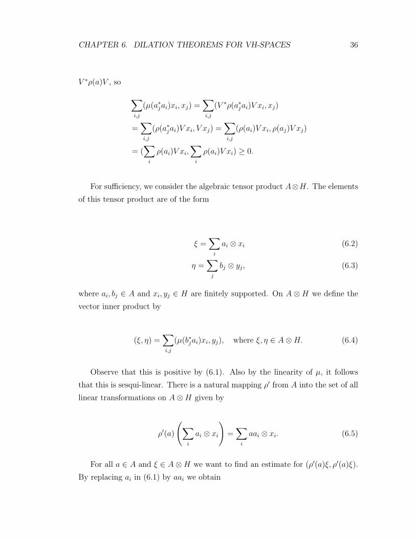
V ∗ρ(a)V , so

∑i,j

(µ(a∗jai)xi, xj) =∑i,j

(V ∗ρ(a∗jai)V xi, xj)

=∑i,j

(ρ(a∗jai)V xi, V xj) =∑i,j

(ρ(ai)V xi, ρ(aj)V xj)

= (∑i

ρ(ai)V xi,∑i

ρ(ai)V xi) ≥ 0.

For sufficiency, we consider the algebraic tensor product A⊗H. The elements

of this tensor product are of the form

ξ =∑i

ai ⊗ xi (6.2)

η =∑j

bj ⊗ yj, (6.3)

where ai, bj ∈ A and xi, yj ∈ H are finitely supported. On A ⊗H we define the

vector inner product by

(ξ, η) =∑i,j

(µ(b∗jai)xi, yj), where ξ, η ∈ A⊗H. (6.4)

Observe that this is positive by (6.1). Also by the linearity of µ, it follows

that this is sesqui-linear. There is a natural mapping ρ′ from A into the set of all

linear transformations on A⊗H given by

ρ′(a)

(∑i

ai ⊗ xi

)=∑i

aai ⊗ xi. (6.5)

For all a ∈ A and ξ ∈ A⊗H we want to find an estimate for (ρ′(a)ξ, ρ′(a)ξ).

By replacing ai in (6.1) by aai we obtain


∑i,j

(µ(a∗ja∗aai)xi, xj) ≥ 0. (6.6)

We know that the following inequality holds in a C∗-algebra

− ‖a∗a‖ ≤ a∗a ≤ ‖a∗a‖. (6.7)

Then it follows that ‖a∗a‖ − a∗a ≥ 0. In a C∗-algebra any positive element is

of the form v∗v for some v. This allows us to replace a∗a in (6.6) by ‖a∗a‖− a∗a.

By the linearity of µ this yields

∑i,j

(µ(a∗ja∗aai)xi, xj) ≤ ‖a∗a‖

∑i,j

(µ(a∗jai)xi, xj), (6.8)

equivalently,

(ρ′(a)ξ, ρ′(a)ξ) ≤ ‖a‖2(ξ, ξ) (6.9)

which is the estimate we need.

We define N = ξ ∈ A ⊗ H | (ξ, ξ) = 0 . N is a linear manifold by

Lemma 3.10. Also, N is invariant under ρ′(a) by (6.9). Hence, the quotient space

(A⊗H)/N is a V E-space. By taking the abstract completion of a VE-space, as

we explained in the preliminaries, we obtain the VH-space K. By using (6.9) we

can extend ρ′ to ρ in the completion.

We define V x = 1⊗x+ N for all x ∈ K. We have (1⊗x, 1⊗x) = (µ(1)x, x).

Since (µ(1)x, x) ≥ 0 by (6.1), as in the proof of Theorem 3.11 we have

2(µ(1)x, x) = (µ(1)x, x) + (x, µ(1)x) ≤ (µ(1)x, µ(1)x) + (x, x)

≤ (‖µ(1)‖2 + 1)(x, x)

from which it follows that V is a bounded operator. Different from the standard

case it is not clear here why V should be adjointable. But since µ is adjointable

it turns out that we can find the adjoint of V too: V ∗(a⊗y) = µ∗(a∗)y. We check


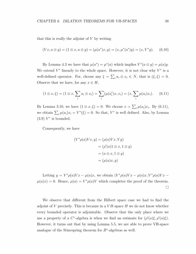
that this is really the adjoint of V by writing

(V x, a⊗ y) = (1⊗ x, a⊗ y) = (µ(a∗)x, y) = (x, µ∗(a∗)y) = (x, V ∗y). (6.10)

By Lemma 4.3 we have that µ(a∗) = µ∗(a) which implies V ∗(a⊗ y) = µ(a)y.

We extend V ∗ linearly to the whole space. However, it is not clear why V ∗ is a

well-defined operator. For, choose any ξ =∑

i ai ⊗ xi ∈ N , that is (ξ, ξ) = 0.

Observe that we have, for any x ∈ H,

(1⊗ x, ξ) = (1⊗ x,∑i

ai ⊗ xi) =∑i

(µ(a∗i )x, xi) = (x,∑i

µ(ai)xi). (6.11)

By Lemma 3.10, we have (1 ⊗ x, ξ) = 0. We choose x =∑

i µ(ai)xi. By (6.11),

we obtain∑

i µ(ai)xi = V ∗(ξ) = 0. So that, V ∗ is well defined. Also, by Lemma

(3.9) V ∗ is bounded.

Consequently, we have

(V ∗ρ(a)V x, y) = (ρ(a)V x, V y)

= (ρ′(a)1⊗ x, 1⊗ y)

= (a⊗ x, 1⊗ y)

= (µ(a)x, y)

Letting y = V ∗ρ(a)V x − µ(a)x, we obtain (V ∗ρ(a)V x − µ(a)x, V ∗ρ(a)V x −µ(a)x) = 0. Hence, µ(a) = V ∗ρ(a)V which completes the proof of the theorem.

We observe that different from the Hilbert space case we had to find the

adjoint of V precisely. This is because in a V H-space H we do not know whether

every bounded operator is adjointable. Observe that the only place where we

use a property of a C∗-algebra is when we find an estimate for (ρ′(a)ξ, ρ′(a)ξ).

However, it turns out that by using Lemma 5.5, we are able to prove VH-space

analogue of the Stinespring theorem for B∗-algebras as well.


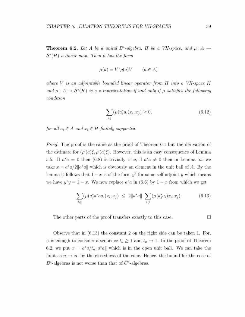
Theorem 6.2. Let A be a unital B∗-algebra, H be a VH-space, and µ : A →B∗(H) a linear map. Then µ has the form

µ(a) = V ∗ρ(a)V (a ∈ A)

where V is an adjointable bounded linear operator from H into a VH-space K

and ρ : A → B∗(K) is a ∗-representation if and only if µ satisfies the following

condition

∑i,j

(µ(a∗jai)xi, xj) ≥ 0, (6.12)

for all ai ∈ A and xi ∈ H finitely supported.

Proof. The proof is the same as the proof of Theorem 6.1 but the derivation of

the estimate for (ρ′(a)ξ, ρ′(a)ξ). However, this is an easy consequence of Lemma

5.5. If a∗a = 0 then (6.8) is trivially true, if a∗a 6= 0 then in Lemma 5.5 we

take x = a∗a/2‖a∗a‖ which is obviously an element in the unit ball of A. By the

lemma it follows that 1− x is of the form y2 for some self-adjoint y which means

we have y∗y = 1− x. We now replace a∗a in (6.6) by 1− x from which we get

∑i,j

(µ(a∗ja∗aai)xi, xj) ≤ 2‖a∗a‖

∑i,j

(µ(a∗jai)xi, xj). (6.13)

The other parts of the proof transfers exactly to this case.

Observe that in (6.13) the constant 2 on the right side can be taken 1. For,

it is enough to consider a sequence tn ≥ 1 and tn → 1. In the proof of Theorem

6.2, we put x = a∗a/tn‖a∗a‖ which is in the open unit ball. We can take the

limit as n → ∞ by the closedness of the cone. Hence, the bound for the case of

B∗-algebras is not worse than that of C∗-algebras.


6.2 A Comparison of Dilation Theorems for

VH-Spaces

In Chapter 4 we obtained Corrollary 4.4 which is a stronger version of Theorem

4.1. In the preceeding section we proved analogs of Stinespring Theorem for

the case of B∗ and/or C∗-algebras and VH-spaces. In this section we prove the

equivalence of these theorems.

Theorem 6.3. Corollary 4.4 implies Theorem 6.1.

Proof. A C∗-algebra A is also a ∗-semigroup. The boundedness condition (4.19)

is obtained in exactly the same way as in the proof of Theorem 6.1. So, we can

use Loynes’s Theorem for ϕ = µ and Φ = ρ. The only point which is not clear

is that why would the map ρ be linear. µ is linear and we put ϕ = µ in the

Loynes Theorem. By Corollary 4.2 we obtain, for t, u, t+ u ∈ A, ϕ(x(t+ u)y) =

ϕ(xty) + ϕ(xuy) which implies that Φ(t + u) = Φ(t) + Φ(u). Hence ρ is also

linear.

Theorem 6.4. Corollary 4.4 implies Theorem 6.2.

Proof. The boundedness condition (4.19) is obtained as in the proof of Theorem

6.2. The other parts of the proof is same as the previous theorem.

An important point here is that whether the converse of Theorem 6.4 holds.

The converse of this theorem holds for the Hilbert space case as we demonstrated

in Chapter 5. We will show that the converse of Theorem 6.4 also holds for the

VH-space case. However, we need the following lemma:

Lemma 6.5. Let ϕ be a map from a ∗-semigroup to B∗(H) for some VH-Space

H. Suppose that ϕ satisfies

2∑i,j=1

(ϕ(s∗i sj)fj, fi) ≥ 0 (6.1)

namely, ϕ is 2-positive. Then, it follows that


(ϕ(s)f, ϕ(s)f) ≤ ‖ϕ(1)‖(ϕ(s∗s)f, f) s ∈ S, f ∈ H. (6.2)

Proof. In (6.1), by letting s1 = 1, s2 = a, f1 = −ϕ(a)f, f2 = ‖ϕ(1)‖f we obtain

(ϕ(1)ϕ(a)f, ϕ(a)f)−‖ϕ(1)‖(ϕ(a)f, ϕ(a)f)− (6.3)

‖ϕ(1)‖(ϕ(a∗)ϕ(a)f, f)+‖ϕ(1)‖2(ϕ(a∗a)f, f) ≥ 0.

By Lemma 4.3 we have ϕ(1∗) = ϕ(1) = ϕ(1)∗, so that ϕ(1) is self-adjoint. By

applying Theorem 3.11 we get

(ϕ(1)ϕ(a)f, ϕ(a)f) ≤ ‖ϕ(1)‖(ϕ(a)f, ϕ(a)f). (6.4)

Replacing the first term of (6.3) by the right side of (6.4), after the cancellations,

gives us

(ϕ(a∗)ϕ(a)f, f) ≤ ‖ϕ(1)‖(ϕ(a∗a)f, f).

Since we have ϕ(a∗) = ϕ(a)∗ by Lemma 4.3 we obtain,

(ϕ(a)f, ϕ(a)f) ≤ ‖ϕ(1)‖(ϕ(a∗a)f, f).

Hence, the result.

Observe that we can apply Lemma 6.5 if ϕ is positive definite. Since any

positive definite map is 2-positive.

Theorem 6.6. Theorem 6.2 implies Corollary 4.4.

Proof. By the c(u)-boundedness in Corollary 4.4 we have

(ϕ(s∗u∗us)f, f) ≤ c(u)2(ϕ(s∗s)f, f). (6.5)

Letting s = 1 yields


(ϕ(u∗u)f, f) ≤ c(u)2(ϕ(1)f, f). (6.6)

As in the proof for the Hilbert space case, we take c(u) to be the maximum

of the best constant satisfying the c(u)-inequality (6.5) and 1. Twice application

of the same inequality gives us c : S 7→ [1,∞) to be submultiplicative.

By using (6.2) we obtain

‖ϕ(s)‖ ≤ ‖ϕ(1)‖c(s). (6.7)

Here in defining the B∗-algebra `1(S, c) we proceed exactly the same as in the

proof Stinespring’s Theorem ⇒ Sz.-Nagy’s Theorem in Chapter 5. We define a

map ϕ : l1(S, c) → B∗(H) as ϕ(ξ) =∑

s ξ(s)ϕ(s). In Chapter 5 it was checked

that ϕ satisfies positive definiteness which also applies to here. Also, similar to

the Hilbert space case by using (6.7) we obtain

‖ϕ(ξ)‖ ≤ ‖ϕ(1)‖‖ξ‖. (6.8)

However, the positive definiteness was checked only for functions ξ which vanishes

all but only finitely many points. Because any function can be norm approximated

by such functions, in order to check the positive definiteness of ϕ for any function

we consider finitely supported sequences such that ξ(n)i → ξi as n goes to infinity.

We have that ∑i,j

(ϕ(ξ(n)∗jξ(n)i)xi, xj) ≥ 0.

Since `1(S, c) is a Banach space we have, if ξ(n)∗j → ξ∗j and ξ(n)i → ξi it follows

that ξ(n)∗jξ(n)i → ξ∗j ξi. This is clear by the fact that

‖ξ(n)∗jξ(n)i − ξ∗j ξ(n)i + ξ∗j ξ(n)i − ξ∗j ξi‖

≤ ‖ξ(n)i‖‖ξ(n)∗j − ξ∗j ‖+ ‖ξ∗j ‖‖ξ(n)i − ξi‖

By (6.8) we have that ϕ(ξ(n)∗jξ(n)i)→ ϕ(ξ∗j ξi). The continuity of inner product


gives

∑i,j

(ϕ(ξ(n)∗jξ(n)i)xi, xj) −→∑i,j

(ϕ(ξ∗j ξi)xi, xj).

as n → ∞. Since each term∑

i,j(ϕ(ξ(n)∗jξ(n)i)xi, xj) ≥ 0, by the closedness of

the cone we obtain∑

i,j(ϕ(ξ∗j ξi)xi, xj) ≥ 0.

Observe that we have a way back to ϕ by putting ϕ(s) = ϕ(δs) where δs is the

point mass at s. We can apply Theorem 6.2 to ϕ in order to get the representation

(4.17) in Corollary 4.4.

Proposition 6.7. Using the notation in Theorem 6.6 and its proof, we have that

∑i,j

(ϕ(ξ∗j ξi)fi, fj) ≤ ‖ϕ(1)‖

(∑i

‖ξi‖2(fi, fi))

).

Proof. By the definition of ϕ as in the proof of Theorem 6.6 we have

∑i,j

(ϕ(ξ∗j ξi)fi, fj) =∑i,j

(∑s∗,t

(ϕ(s∗t)ξi(t)fi, ξj(s)fj). (6.9)

Throughout the proof we will mainly refer to the right side of (6.9), which we

denote by Σ. Since, ϕ is positive definite it follows that Σ ≥ 0 hence Σ = Σ∗.

Now we consider, Σ + Σ∗ and apply (3.2), for p ≥ 0,

(u, v) + (v, u) ≤ p(u, u) + p−1(v, v)

to the adjoint terms in Σ and Σ∗. So that we have,

2∑i,j

∑s∗,t

(ϕ(s∗t)ξi(t)fi, ξj(s)fj)

≤∑i,j

∑s∗,t

p(ϕ(s∗t)ξi(t)fi, ϕ(s∗t)ξi(t)fi) + p−1(ξj(s)fj, ξj(s)fj)

≤∑i,j

∑s∗,t

p‖ϕ(s∗t)‖2‖ξi(t)‖2(fi, fi) + p−1‖ξj(s∗)‖2(fj, fj). (6.10)


Since by (6.7) we have,

‖ϕ(s∗t)‖2 ≤ ‖ϕ(1)‖2c(s∗)2c(t)2 (6.11)

by using the submultiplicativity of c(s). By plugging (6.11) in (6.10) and putting

p = 1‖ϕ(1)‖c(s∗)2 we obtain,

∑i,j

∑s∗,t)

p‖ϕ(s∗t)‖2‖ξi(t)‖2(fi, fi) + p−1‖ξj(s∗)‖2(fj, fj)

≤∑i,j

∑s∗,t

‖ϕ(1)‖c(t)2‖ξi(t)‖2(fi, fi) + ‖ϕ(1)‖c(s∗)2‖ξj(s∗)‖2(fj, fj)

≤∑i,j

‖ϕ(1)‖

(∑t

c(t)|ξi(t)|

)(∑t

c(t)|ξi(t)|

)(fi, fi)

+ ‖ϕ(1)‖

(∑s∗

c(s∗)|ξj(s∗)|

)(∑s∗

c(s∗)|ξj(s∗)|

)(fj, fj)

So that we have,

≤ ‖ϕ(1)‖∑i

‖ξi‖2(fi, fi) + ‖ϕ(1)‖∑j

‖ξj‖2(fj, fj)

= 2‖ϕ(1)‖

(∑i

‖ξi‖2(fi, fi))

).

where ‖ξ‖ is the norm of ξ in `1(S, c) as mentioned in the proof of Theorem 5.3.

Bibliography

[1] W.A. Arveson, A Short Course on Spectral Theory, Graduate Texts in

Mathematics, 209. Springer-Verlag, New York, 2002.

[2] W.B. Arveson, Dilation theory yesterday and today, preprint 2009,

arXiv:0902.3989

[3] J.B. Conway, A Course in Operator Theory, Graduate Studies in Mathe-

matics, 21. American Mathematical Society, Providence, RI, 2000.

[4] J.B. Conway, A Course in Functional Analysis Second edition. Graduate

Texts in Mathematics, 96. Springer-Verlag, New York, 1990.

[5] J. Dixmier, C∗-Algebras, North-Holland Mathematical Library, Vol. 15.

North-Holland Publishing Co., Amsterdam-New York-Oxford, 1977.

[6] E.C. Lance, Hilbert C∗-Modules. A toolkit for operator algebraists, London

Mathematical Society Lecture Note Series, 210. Cambridge University Press,

Cambridge, 1995.

[7] R.M. Loynes, On generalized positive-definite functions, Proc. London

Math. Soc. III. Ser. 15(1965), 373–384.

[8] R.M. Loynes, Linear operators in V H-spaces, Trans. Amer. Math. Soc.

116(1965), 167–180.

[9] R.M. Loynes, Some problems arising from spectral analysis, in Symposium

on Probability Methods in Analysis (Loutraki, 1966), pp. 197–207, Springer,

Berlin 1967.

45

BIBLIOGRAPHY 46

[10] A.P. Robertson, Wendy Robertson, Topological Vector Spaces, Cam-

bridge University Press, Cambridge, 1973.

[11] W.F. Stinespring, Positive functions on C∗-algebras, Proc. Amer. Math.

Soc. 6(1955). 211–216.

[12] F.H. Szafraniec, Dilations on involution semigroups. Proc. Amer. Math.

Soc. 66(1977), no. 1, 30–32.

[13] F.H. Szafraniec, Note on a general dilation theorem. Pol.Math. 36(1979),

43–47.

[14] F.H. Szafraniec, Dilations of linear and nonlinear maps, in Functions,

series, operators, Vol. I, II (Budapest, 1980), pp. 1165–1169, Colloq. Math.

Soc. Jnos Bolyai, 35, North-Holland, Amsterdam, 1983.

[15] B. Sz.-Nagy, Prolongement des transformations de l’espace de Hilbert qui

sortent de cet espace, in Appendice au livre “Lecons d’analyse fonctionnelle”

par F. Riesz et b. Sz.-Nagy, pp.439-573 Akadmiai Kiad, Budapest, 1955.

dilation theorems for vh-spaces · abstract dilation theorems for vh-spaces bar ˘s evren u gurcan...

Documents