DISCUSSION PAPER SERIES

IZA DP No. 10722

Marion CollewetJan Sauermann

Working Hours and Productivity

APRIL 2017

Any opinions expressed in this paper are those of the author(s) and not those of IZA. Research published in this series may include views on policy, but IZA takes no institutional policy positions. The IZA research network is committed to the IZA Guiding Principles of Research Integrity.The IZA Institute of Labor Economics is an independent economic research institute that conducts research in labor economics and offers evidence-based policy advice on labor market issues. Supported by the Deutsche Post Foundation, IZA runs the world’s largest network of economists, whose research aims to provide answers to the global labor market challenges of our time. Our key objective is to build bridges between academic research, policymakers and society.IZA Discussion Papers often represent preliminary work and are circulated to encourage discussion. Citation of such a paper should account for its provisional character. A revised version may be available directly from the author.

Schaumburg-Lippe-Straße 5–953113 Bonn, Germany

Phone: +49-228-3894-0Email: publications@iza.org www.iza.org

IZA – Institute of Labor Economics

DISCUSSION PAPER SERIES

IZA DP No. 10722

Working Hours and Productivity

APRIL 2017

Marion CollewetCORE, Universite Catholique de Louvain and ROA, Maastricht University

Jan SauermannSOFI, Stockholm University, CCP, IZA and ROA

ABSTRACT

APRIL 2017IZA DP No. 10722

Working Hours and Productivity*

This paper studies the link between working hours and productivity using daily information

on working hours and performance of a sample of call centre agents. We exploit variation

in the number of hours worked by the same employee across days and weeks due to

central scheduling, enabling us to estimate the effect of working hours on productivity. We

find that as the number of hours worked increases, the average handling time for a call

increases, meaning that agents become less productive. This result suggests that fatigue

can play an important role, even in jobs with mostly part-time workers.

JEL Classification: J23, J22, M12, M54

Keywords: working hours, productivity, output, labour demand

Corresponding author:Marion CollewetCenter for operations research and econometrics (CORE)Universite Catholique de LouvainVoie du Roman Pays 34/L1.03.011348 Louvain-la-NeuveBelgium

E-mail: marion.collewet@uclouvain.be

* The authors would like to thank Jordi Blanes-I-Vidal, Alexandra de Gendre, Andries De Grip, Annemarie Künn-Nelen, John Pencavel, two anonymous referees, and seminar participants at the Paris School of Economics, and audience at EALE 2016 for valuable comments and suggestions. Jan Sauermann gratefully acknowledges financial support from the Jan Wallanders och Tom Hedelius Stiftelse for financial support (Grant number I2011-0345:1).

1 Introduction

Hours worked vary substantially between countries, but also within countries,

e.g. due to the prevalence of part-time work and working hours regulations or

agreements (Bick et al., 2016; OECD, 2016). Understanding how the num-

ber of hours worked affects labour productivity is an important element of

understanding labour demand, and has important implications for the regu-

lation of working hours and firm management. Still, a lot remains unknown

about the effect of working hours on labour productivity. In theory, there

could be two opposite effects. On the one hand, longer hours can lead to

higher productivity if a worker faces fixed set-up costs and fixed unproduc-

tive time during the day, or if longer hours lead to better utilisation of capital

goods (Feldstein, 1967). On the other hand, worker fatigue could set in af-

ter a number of hours worked, so that the marginal effect on productivity

of an extra hour per worker starts decreasing (Pencavel, 2015). If neither

of these effects apply, or if both cancel each other out, it could also be the

case that marginal productivity does not change with working time, so that

output is proportional to the number of hours worked. Identifying the effect

of working time on productivity is not straightforward for two main reasons.

First, unobservable characteristics of industries, firms, jobs and individuals

are likely to influence both working time and productivity, so that the cor-

relation between the two variables is likely to be a biased estimate of the

effect of working time on productivity. Second, external shocks could in-

fluence both working time and productivity, which again leads to a biased

estimation of the effect.

In this paper, we study the influence of the daily number of hours worked

on workers’ productivity using panel data from a call centre in the Nether-

lands from mid-2008 to the first week of 2010 (cf. De Grip and Sauermann,

2012; De Grip et al., 2016). For each of the 332 workers in our sample, the

data contain detailed information on the number of daily working hours, and

workers’ individual performance, as measured by the average handling time

of calls. The panel structure of our data set allows us to correct for time-

invariant unobserved characteristics of individuals that may influence both

1

working time and productivity. Moreover, the exact number of hours worked

by a worker on a given day is determined by central planning. Expected cus-

tomer demand determines the scheduling process, and schedules are hardly

related to individual preferences. This enables us to obtain estimates of the

effect of working time on productivity.

Estimating a model controlling for individual fixed effects and several

types of time fixed effects, we find that an increase in working hours by

1 percent leads to an increase in output by only 0.9 percent, measured as

the number of calls answered. This finding suggests that fatigue sets in

as working time increases. The corresponding decrease in productivity is

mild in this sample where most employees work part-time, but it suggests

that fatigue effects would be much stronger if agents would work full-time.

We find evidence of more strongly decreasing returns to hours for workers

with shorter tenure, a result that is not driven by worker attrition. Using

additional data on service quality, we find that longer working hours are

associated with a moderate increase of call quality in working hours, a result

that partly offsets the negative effect on the number of calls answered.

This paper contributes to a rich literature that studies the link between

working time and productivity. Studies estimating production functions

based on industry-level data find mixed evidence for the returns to work-

ing hours. Whereas some studies find increasing returns to hours (Feldstein,

1967; Craine, 1973; Leslie, 1984), which could be the result of not taking

capacity utilisation rates into account (e.g. Tatom, 1980), or be due to ag-

gregation bias (e.g. DeBeaumont and Singell, 1999), other studies conclude

that output is roughly proportional to hours worked per worker (Hart and

McGregor, 1988; Anxo and Bigsten, 1989; Ilmakunnas, 1994). The majority

of studies, however, find evidence of decreasing returns to hours (e.g. Leslie

and Wise, 1980; Tatom, 1980; DeBeaumont and Singell, 1999; Shepard and

Clifton, 2000). Typically, studies using aggregate data deal with the endo-

geneity of working time by using panel data and including industry fixed

effects, and by instrumenting for working time using lagged values or ranks.

The validity of such instruments, however, can be questioned, and the mea-

2

surement of working time and output at these aggregate levels is likely to be

subject to error.

Studies using firm-level data, or data from workers in individual firms

or in specific sectors are typically better at dealing with the endogeneity of

working hours. A few studies use panels of firms to estimate the link between

working time and firm or establishment productivity (Crepon et al., 2004;

Schank, 2005; Kramarz et al., 2008; Gianella and Lagarde, 2011). They

tend to find that output is roughly proportional to the number of hours

worked.1 Due to the data structure, these studies are able to control for the

endogeneity of working time caused by time-invariant firm characteristics.

However, shocks that would affect both working time and productivity could

still form a potential source of bias.

Studies using data about individual workers in a firm, or about work-

ers in comparable firms date back to the early 20th century, when studies

descriptively analysed the relationship between working hours and output,

or compared output before and after a change in working hours (Goldmark,

1912; Vernon, 1921; Kossoris, 1947).2 More recent studies, however, exploit

exogenous sources of variation in working hours to address the relationship

between hours and worker level productivity. An early example is the study

of citrus harvesters by Crocker and Horst (1981), who use the size of the

grove worked on as a source of variation in working time. Brachet et al.

(2012) conduct a difference-in-differences analysis to compare performance

of paramedics working on short and long shifts. Using data from munition

plants in Britain during the First World War, Pencavel (2015) uses vari-

ation in working time coming from the demand for shells to estimate the

effect of working time on productivity. Dolton et al. (2016) use data from

the Hawthorne experiments (conducted between 1924 and 1932) to exploit

1Crepon et al. (2004) and Kramarz et al. (2008) find positive effects on productivityof participating in a working time reduction scheme for French firms, but this effect isdue to the reorganisation of work that took place as a consequence of the working timereduction. Work allocation as a mechanism to explain the link between part-time work andproductivity has been studied by Kunn-Nelen et al. (2013), Specchia and Vandenberghe(2013), Garnero et al. (2014), and Devicienti et al. (2015).

2See Nyland (1989) for an overview of these and other studies.

3

the fact that workers were subjected to different working times in different

periods. While Crocker and Horst (1981) find that output is proportional

to hours worked, Brachet et al. (2012), Pencavel (2015), and Dolton et al.

(2016) find evidence of decreasing returns to hours. A contrasting result is

found by Lu and Lu (2016), who exploit changes in mandatory overtime laws

for nurses. They find that the introduction of overtime laws actually reduced

the quality provided by nurses, an effect that can be explained by changes in

staffing policies of permanent and contractual (temporary) nurses.3 We con-

tribute to this literature by exploiting exogenous variation in working hours,

which is due to the call centre’s central scheduling.

Most of the studies that are able to exploit exogenous variation in working

time to identify the effect of working hours on productivity have concentrated

on either manual workers from the first half of the 20th century (Pencavel,

2015; Dolton et al., 2016)4, or on the health sector using more recent data

(Brachet et al., 2012; Lu and Lu, 2016). In this paper, we provide evidence

about call agents in a call centre. Our results can have informative value for

a broader range of medium-skilled level jobs in the service sector, and are

relevant for policies such as working time regulation.

The remainder of the paper is structured as follows. In the next section,

we outline our conceptual framework. Section 3 presents the empirical model

we estimate and our identification strategy. Section 4 describes the data we

use. Section 5 presents our main estimation results. In Section 6, we conduct

a number of robustness checks, and we formulate conclusions in Section 7.

3In addition to these studies, there are more studies for the health sector, typicallyfinding decreasing returns to working hours. These studies, however, are either based onindirect performance measures (psychometric tests, simulations of work tasks, self-reportquestionnaires; for a review, see Kodz et al., 2003), or on correlations and before-aftercomparisons (Rogers et al., 2004; Hart and Krall, 2007; McClay, 2008). There is also arelated literature that has analysed the link between long working hours and health (e.g.van der Hulst, 2003) and between long hours and occupational injuries (e.g. Vegso et al.,2007; Lee and Lee, 2016). These studies suggest that working long hours is detrimentalfor health and therefore may have negative effects on productivity.

4The relation between working time and productivity might have changed as the natureof jobs evolved. Pencavel concludes his paper stating that “it would be valuable if theanalysis here could be repeated on contemporary data that contain information on workers’output and their working hours” (p. 2074).

4

2 Conceptual framework

2.1 Model

Typically, studies of the relation between working time and productivity

estimate a model of the type:

Y = f(H,X) + ε (1)

where Y is a measure of output, H a measure of hours worked, X is a

set of variables which are also relevant for output (the capital stock being

a typical candidate), and ε is the error term. Very often, the relationship

between log output and log hours is estimated assuming a Cobb-Douglas

production function. Because we focus on productivity at the level of the

individual worker, for whom capital use is constant (namely one workstation),

the Cobb-Douglas function can be estimated as

ln(Y ) = α · ln(H) + γ ·X + ε (2)

In our setting, call centre management uses a specific measure to evaluate

the performance of its agents: average handling time (AHT ), which is based

on the time taken by an individual agent to answer each call during a given

day or a given week. If output Y is defined as the number of calls made on

a given day, it can be expressed as

Y =H

AHT(3)

Inserting Equation (3) into (2) gives:

ln(AHT ) = (1 − α) · ln(H) − γ ·X − ε (4)

Average handling time is a negative measure of productivity, since indi-

viduals who take more time to answer calls are less productive (cf. De Grip

and Sauermann, 2012). To facilitate direct interpretation of our estimation

results, we multiply Equation (4) by −1, which allows us to rewrite it to

5

ln(

1

AHT

)= (α− 1) · ln(H) + γ ·X + ε (5)

and to use 1/AHT as a measure of productivity: an increase in 1/AHT can

therefore be interpreted as an increase in productivity.

In this model, a coefficient on ln(H) equal to zero indicates that work-

ers’ productivity does not vary with working hours, which is equivalent to

constant returns to hours. A positive coefficient corresponds to increasing

returns to hours, and a negative one to decreasing returns. The magnitude

of the coefficient on log hours is also directly interpretable: as hours increase

by 1 percent, output increases by α percent. If we define the coefficient on

ln(H) to be β = α − 1, output increases by β + 1 percent as hours increase

by 1 percent.

We estimate the model both at the day and at the week level to address

potential heterogeneity in the returns to working hours at the day and week

level: at the week level, workers have time to recover from one day to another,

so that returns to hours might be more positive than at the day level (cf.

Pencavel, 2016). Moreover, comparing returns to hours at the day and at the

week level can tell us whether productivity can be increased by distributing

weekly working hours differently across days.

2.2 Mechanisms

Before turning to estimating the model, we want to pay closer attention to

the mechanisms that link working hours to labour productivity. Why exactly

would we expect labour productivity to rise or fall as working hours increase?

Potential reasons for increasing returns to hours are fixed unproductive

time and better capital utilisation rates. In our setting, unproductive time

cannot play a role because we study effective working time (excluding breaks,

see Section 4). Capital utilisation rates are not relevant either because we

focus on the level of the individual worker, who always uses exactly one

workstation consisting of a phone and a computer. One possible mechanism

that could lead productivity to increase with working time is what Vernon

(1921) calls “practice-efficiency”, i.e. the fact that one gets better at a task

6

as one “warms up”.5 It is an open question whether what he describes for

physical work may also apply to call centre agents.

The main reason why productivity would decrease as working hours in-

crease is worker fatigue.6 The origins of the literature on fatigue and the

link between working hours and labour productivity lie in the study of the

manufacturing industry in the early 20th century (Goldmark, 1912; Vernon,

1921), with physically demanding jobs and very long hours. But fatigue is

still relevant in today’s service economy with shorter hours. Indeed, Ny-

land (1989) emphasizes that the fall in working hours over the course of the

twentieth century has been accompanied by an intensification of work due

to the rise of scientific management, so that the optimal number of working

hours has most probably dropped below levels that were recommended at the

beginning of the twentieth century. In fact, the majority of studies on the

link between working hours and productivity still finds decreasing returns

to hours. Moreover, physical demands are not the only demands of a job.

Goldmark (1912) already emphasises the important role played by speed and

complexity of a task.7 Bakker et al. (2003) find that job demands are related

to exhaustion and repetitive strain injury in call centre agents. The agents

we study were exposed to a constant flow of incoming calls and had to solve

problems that were potentially different for every single call. The manage-

5“The complex chain of central nervous system, neuro-muscular mechanisms, nervesand muscles involved takes time to work up to its maximum efficiency, and to get intothorough running order. In fact, this efficiency is unattainable except by practice, henceI have termed it practice-efficiency.” (Vernon, 1921, p. 13).

6Vernon (1921) cites the definition by the British Association Committee on Fatiguefrom the Economic Standpoint: it sees fatigue as the “diminution of the capacity for workwhich follows excess of work or lack of rest, and which is recognised on the subjective sideby a characteristic malaise.” (p.1). More recently, in the occupational health literature,fatigue is defined by van Dijk and Swaen (2003) as “the change in the psychophysiologicalcontrol mechanism that regulates task behaviour, resulting from preceding mental and/orphysical efforts which have become burdensome to such an extent that the individual isno longer able to adequately meet the demands that the job requires of his or her mentalfunctioning; or that the individual is able to meet these demands only at the cost ofincreasing mental effort and the surmounting of mental resistance.”

7Interestingly, she takes telephone operators as an example, and reports that a medicalcommission deemed a 7-hours workday too long for “telephone girls”. Of course, it has tobe said that the work of telephone operators was much more physically demanding thanthe work of call centre agents today.

7

ment of the call centre seemed well aware of the intensity and difficulty of the

task agents had to perform: without having actually measured the relation

between working hours and productivity, they expected a full-time contract

to be sub-optimal in terms of productivity and preferred to offer part-time

contracts to their employees for that reason.

3 Empirical strategy

Using panel data, our empirical model can be written as

ln(

1

AHTit

)= φ+ β · ln(Hit) + γ ·Xit + δ · Tt + µi + εit (6)

where the subscript i stands for an individual agent, and t represents the

time period (day or week) examined. In this section, we first discuss how we

control for potential confounders, and second how we exploit scheduling as

a source of exogenous variation in working hours.

3.1 Controlling for potential confounders

As mentioned above, there are several factors that can result in a biased esti-

mate of the effect of hours on productivity (β). First, the estimate could be

biased due to characteristics of individuals that influence both their working

time and their productivity, such as preferences or ability. As far as these

individual characteristics are time-invariant, they can be controlled for by

the individual fixed effect µi in our model. Taking account of this unob-

served heterogeneity takes away an important part of the potential bias in

the coefficient on ln(Hit).

Second, the timing of work might be important as well. If variation

in types or amounts of customer calls varies over time, and this variation

results in changes of agents’ productivity, it is important to control for when

individuals work.8 In estimations at the day level, we control for day of the

8Note that, although we have precise information on when and how long agents areworking, the data only contain information on performance on the daily level, but not bythe hour.

8

week dummies (as part of Tt) and for hours dummies for the time during

which an individual works on a given day (as part of Xit); in estimations

at the week level, we control for 168 dummies that represent each hour of

the week. There might also be shocks on specific days or weeks, e.g. if

there are technical problems that both induce agents to stay longer hours

and affect their productivity because the shocks influence the time taken to

help customers or the pressure experienced by agents. To control for this

possibility, our model includes day fixed effects in regressions based on daily

data, or week fixed effects in regressions based on weekly data.

Third, tenure is a potential confounder. Differences in tenure between

individuals at the beginning of the observation period are captured by the

individual fixed effect. However, as individuals become more experienced,

their productivity is likely to increase, and their working time might also

evolve. If this is the case, some of the effect of tenure will unduly be attributed

to working time. We therefore include a general time trend in the model.

Further, in Section 6, we run additional regressions including individual-

specific time trends, i.e. interactions of the individual fixed effect with the

time trend. This allows us to provide evidence against the hypothesis that

call centre management could give different contracts or schedules to workers

who learn faster.

Fourth, attrition may also be a problem. There is relatively high turnover

in our sample, resulting in that individuals who stay for relatively long in

the sample may be overrepresented in our data. If more productive individ-

uals stay longer, and if they are therefore overrepresented, we will tend to

overestimate returns to hours. We address this problem by estimating our

model for a balanced sub-sample in Section 6. This analysis shows that the

bias caused by attrition is only limited.

Finally, the team in which an individual works may also be a confounder,

in the sense that a team with more positive characteristics (more cohesive,

better team leader, etc.) may both induce an agent to be willing to work

longer hours and make him or her more productive. This would lead to an

underestimation of the fatigue effect, i.e. an overestimation of the returns to

hours. To rule this out, we include team fixed effects in our model.

9

3.2 Exogeneity of working hours due to central schedul-

ing

In our data, variation in an agent’s working time from day to day or from

week to week arises because contractual weekly working time does not need

to be exactly enforced every week. Rather, average working time over a

period of three months should be equal to contractual working time. An

agent’s working time for a given day is defined by the planning department,

on the basis of an algorithm that forecasts customer demand, i.e. the number

of incoming calls. A first version of an agent’s schedule for a given day is

communicated five weeks in advance, but it can be revised up to the last

moment. We also know that earlier performance of agents does not influence

future schedules. In principle, this ensures that the exact number of hours

worked by an individual on a given day is not related to shocks affecting this

individual, so that Hit is not correlated with εit, the idiosyncratic error term.

There are two potential ways in which individual preferences could in the-

ory still influence working time on a given day or a given week. First, agents

are allowed to state preferences about their schedule, both general prefer-

ences and preferences for specific days or weeks, without having a guarantee

that these preferences can be respected. While general preferences stated

by an agent about his or her schedule are captured by the individual fixed

effect, preferences concerning a specific day or week are not. Second, in case

of unexpectedly high or low demand at the last minute, agents are asked to

stay longer or leave earlier on a voluntary basis, with a corresponding ad-

justment in their pay. In theory, these two factors leave some room for the

agents to work more on days on which they expect to be more productive,

leading to an overestimation of the returns to hours. However, these poten-

tial sources of bias do not appear to play an important role in practice. In

Section 6, we present estimations including scheduled hours (or deviations

from schedules) as an additional control variable. This enables us to check

whether, conditional on the actual number of hours worked, schedules (or

deviations from schedules) are still related to productivity, which would hint

at self-selection by agents. We show that there is only very limited evidence

10

of self-selection, and that taking it into account barely changes our results.

We conclude that, conditional on our set of fixed effects, scheduling can be

considered an exogenous source of variation in working hours.

4 Data

4.1 Description of the context

We use rich company data on call agents employed in a call centre located

in the Netherlands. This customer service centre handles calls from current

and prospective customers of a mobile telecommunication company. The call

centre comprises five departments, which are segmented by customer groups.

To focus on workers which have comparable performance, we limit the sample

to the largest department, for customers with fixed contracts.

In this department, all call agents have the same task, answering cus-

tomer calls. Customers call the call centre in case of problems, complaints or

questions and are routed to available agents. Typically, at a given moment,

the number of incoming calls exceeds the number of available agents, gen-

erating non-zero waiting time for customers. Agents who have completed a

call faster are automatically linked to the next customer waiting. This means

that fast agents do not have longer breaks and do not need to wait for the

next customers. Therefore, agents have little slack time when on the job.

In other words, the number of hours that agents spend answering calls, our

main measure of working time, is very close to the number of hours during

which agents are available for calls.

Agents are incentivised to perform, and in particular to handle calls fast.

Agents are organised in 19 teams, each of which is led by a team leader.

The main task of team leaders is to monitor and evaluate the agents of his

or her team. For this purpose, team leaders receive weekly scorecards with

detailed information of their agents’ performance (including average handling

time), and regularly listen to the calls of their agents. Agents receive a fixed

11

wage per hour.9 Following a performance appraisal of the team leader, the

agent receives a grade from 1 (worst) to 5 (best), which determines both

the size of an annual wage increase and an annual bonus. This grade is

determined by both the performance over the year, but also by other, more

subjective factors, such as the behaviour towards co-workers. The maximum

wage increase depends on the firm performance, and does not exceed 8% for

agents with the highest grade.10 Otherwise, there are no explicit incentives

based on agents’ performance, such as piece rates or bonuses upon their daily

or weekly performance.

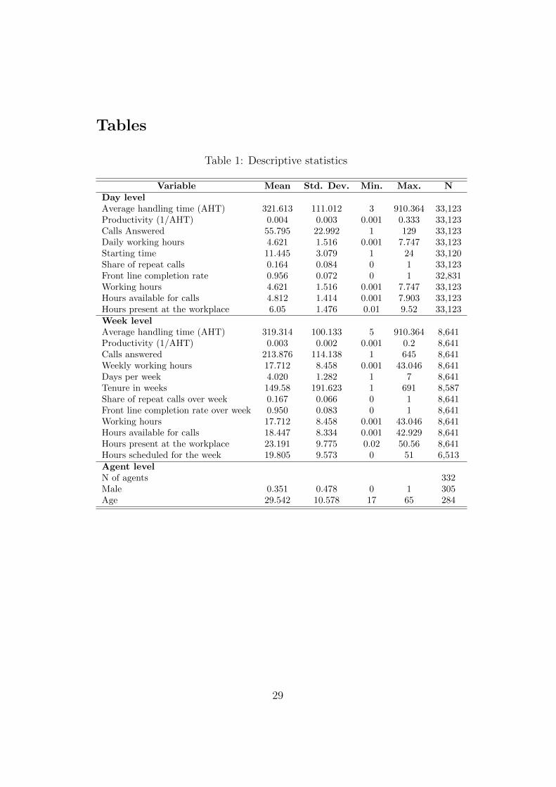
Our data comprise daily performance information for each agent work-

ing in the call centre. In total, our analysis includes 332 agents on 33,123

agent-working days, over an observation period from week 36/2008 to week

1/2010. Descriptive statistics for the estimation sample are provided in Ta-

ble 1. Besides information on performance, the data also contain information

on the working hours and on some basic characteristics of the agents. The

majority of the agents is female, only 35% of all agents are men. Agents are

on average 29 years old, and the average tenure over all observations is about

140 weeks.11

4.2 Measuring performance

The main measure of performance used by the call centre is average handling

time (AHT). It is defined as the time taken for talking to the customer, plus

9Barzel (1973) studies how working hours are determined by the interplay of supplyand demand when the remuneration of an extra hour of work varies together with theproduct of that extra hour. In our setting, workers are paid a constant hourly wage rate,and therefore face the linear budget constraint which is usually assumed in the standardmodel of labour supply. Therefore, our findings about the relation between hours andlabour productivity are mainly relevant for the demand side of the labour market.

10We observe the results of the annual performance appraisals only for a subsample ofagents. In these data, only very few agents receive the worst and the best grade (1: 1.3%;5: 0.7%), while most agents receive a 2 (29.9%), 3 (54.6%), or 4 (13.6%), respectively.The criteria for performance appraisals are agents’ performance scorecards throughoutthe year, as well as the behaviour of the agent towards co-workers and team leader.

11The firm’s administrative data includes a small number of outliers. We therefore keptonly observations with positive values for hours and performance, and excluded from thesample half a percentile at the top of the performance and the working hours distribution.

12

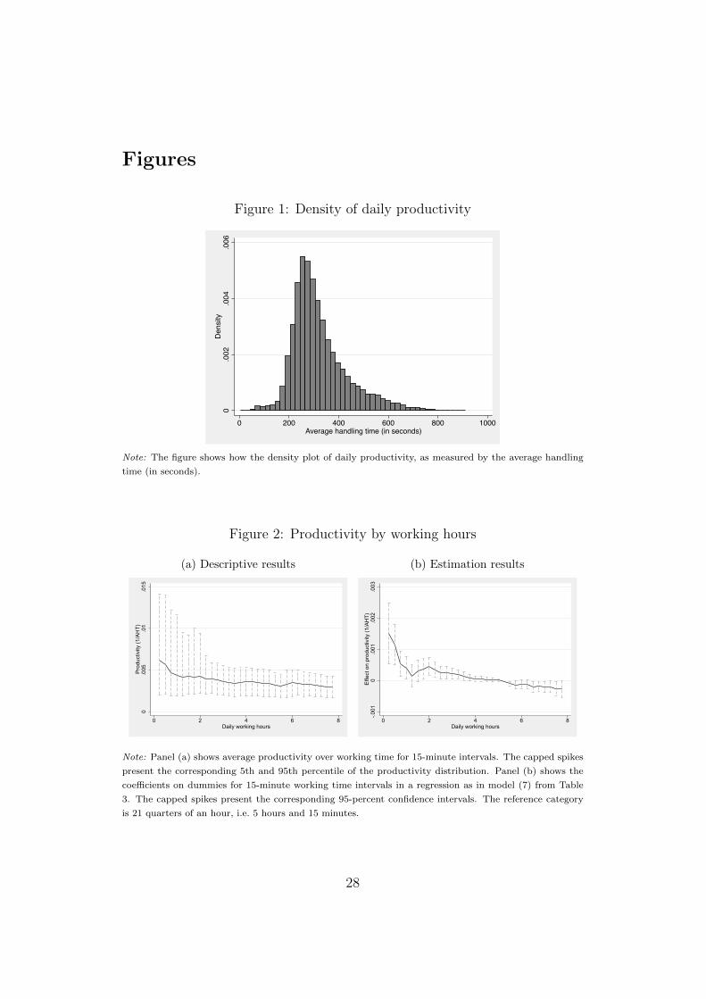
time taken for logging the information in the firm’s database. On average,

agents take 322 seconds, or 5.35 minutes, to handle a call. Figure 1 shows

the density of average handling time and shows that the distribution is right-

skewed. Earlier studies using performance data of call agents have used

similar measures to estimate the impact of training and learning on-the-

job on performance (Liu and Batt, 2007; De Grip and Sauermann, 2012;

Breuer et al., 2013; De Grip et al., 2016). Panel (a) of Figure 2 depicts the

descriptive relationship between our measure of productivity (1/AHT) and

daily working time. Longer working hours seem to be associated with slightly

lower productivity, i.e. slightly longer average handling times.

While it is relatively straightforward to measure how long agents take for

an average call, it is more difficult to measure the quality of these calls. We

use two different measures of quality. The first is the share of repeat calls.

The system tracks when customers are calling again within seven days after

the last call. Based on this information, the system calculates the share of

customers who call back within 7 days, relative to all customers an agent had

contact with. The higher the share of repeat calls, the lower service quality.

Zero repeat calls indicates that none of the customers an agent had contact

with was calling back within seven days. A value of 1 would indicate that

every customer would have called back.12

A second variable, which is used to assess the quality provided by agents,

is front line completion. This variable is based on the inbound and outbound

calls. Since the main task of agents is to receive inbound calls, and outbound

calls should only be necessary if an agent could not complete a case, a lower

front line completion rate is an indicator of lower quality. Completion is

defined as the difference between an agent’s number of inbound calls and

outbound calls, divided by the number of inbound calls. The measure is 1

if an agent does no outbound calls at all. Thus, a value of 1 reflects high

problem-solving ability of the agent.

12One disadvantage of this measure is that customers might have called back for adifferent reason, which might be unrelated to the original call. In this case, the “repeat”call would be wrongly attributed to an agent.

13

4.3 Measuring working time

Working time is calculated as the number of calls handled by an individual

agent, times the agent’s average handling time. It thus measures the time

during which an agent is directly working on his or her main task, answering

customer calls. By definition, this measure does not comprise any non-call

related time, such as breaks, slack, or training hours. We choose this measure

because it serves as a precise measure of effective working time. If we used

a measure which includes slack time and breaks, part of what would be

counted as working time would actually be recovery time. This would lead

to an underestimation of the fatigue effect. Moreover, slack time or time

for breaks is most probably not proportional to the time spent answering

calls. Rules about breaks, for instance, prescribe different break schemes for

different discrete values of time spent at the workplace. Therefore, the share

of time spent in breaks is not constant across values of time spent at the

workplace. This could also lead to bias in the estimated fatigue effect if we

used a measure of working time which includes breaks.13

To analyse how important our choice of the definition of working hours is,

we also consider two alternative measures of working time in our estimations

in the next section. The first is a measure of hours during which the agent is

available to answer calls at his or her desk. The second is a measure of the

time spent by the agent at the workplace, and includes training, the unpaid

lunch break, etc. They are not, however, precise enough to yield reliable

information about slack time and time spent in breaks.

Table 1 also provides summary statistics of these alternative measures of

working time. Both measures are very strongly correlated with the measure

we chose, in particular the time that agents are available for calls (ρ = 0.95).

Most agents working in the call centre work part time. On average, agents

spend 4 days a week and 6 hours per day at their workplace. Their effective

working time, however, only averages 4.6 hours per day, and 17.7 hours per

week.

13It would be very interesting to study the role played by slack time and breaks, andwhether they function as recovery time for workers (cf. Pencavel, 2016). However, thedata we have does not allow us to do so.

14

Table 2 shows that there is sufficient within-agent variation in the number

of hours worked per day and per week. Agents work days of about 5 effective

working hours about half (45.8 percent) of the time. However, during the

rest of the time, they work very different numbers of hours per day, ranging

from about 0 to about 8 hours. At the week level, the number of observations

peaks at around 24 hours a week. About 70 percent of agents in the sample

have at least one working week of that length, but there is still quite some

variation in the length of the working week across observations and agents.

In addition to the information on working hours, the data also contain

information on the total number of scheduled hours for each individual in

each week.

5 Estimation results

In this section, we present the results of estimating the relation between

working hours and productivity. We first address our main measure of pro-

ductivity, ln(1/AHT ), and then the two measures of the quality of calls. As

mentioned above, we conduct the estimations both at the daily and at the

weekly level.

5.1 Working hours and productivity

Table 3 presents estimation results of a regression of productivity on working

hours at the daily level, including different control variables. Regardless of

the specification, productivity appears to decrease slightly as working hours

increase. As the number of controls included in the model increases, the esti-

mated relationship between working time and productivity tends to become

less negative. In particular, controlling for the timing of shifts (day of the

week and hour dummies) leads to a lower estimate of the fatigue effect. This

is because shifts at atypical times, such as nights and weekends, tend to be

both shorter and more productive. There are two likely explanations for this.

First, agents have less calls to handle, creating slack time to rest between

calls. Second, the call centre is open only for very specific types of calls

15

during the night and during the weekend, which could be shorter by nature.

Consequently, fatigue is overestimated when timing is not controlled for.14

Our preferred specification is shown in Column (7). The interpretation of

the coefficient on ln(H), β, is that output increases by β+1 percent as hours

increase by 1 percent (see Subsection 2.1). Therefore, our estimation results

suggest that if working hours increase by 1 percent, the number of calls han-

dled will only increase by 0.9 percent. This suggests that, as agents work

longer hours, fatigue makes agents work slower. The log-log specification ap-

pears to fit the data. The R2 statistic is higher for this specification than for

a linear or a quadratic one. Panel (b) of Figure 2, which plots the coefficients

obtained from a regression of productivity on a set of dummies for 15-minute

working time intervals, and therefore does not impose any functional form on

the data, also hints at a negative logarithmic relationship between working

time and productivity.15 In Column (8), we include individual-level charac-

teristics. The estimates show that, although agents perform less well with

increasing age, tenure significantly improves productivity (cf. De Grip et al.,

2016). The performance of male and female call agents does not, however,

differ significantly.

Table 4 presents regressions of productivity on working time at the week

level. The magnitude of the negative effect appears less important at the

week level, compared to the results at the day level. This could be explained

by the fact that people have the time to rest from one day to another. The

idea that agents have time to recover from one day to the other is further

supported by the fact that we find no relationship between productivity on a

14If we exclude observations, for which the shifts starts before 09:00 or ends after21:00, we obtain very similar results, with a coefficient on log working hours of -0.105***.Likewise, if we exclude observations from Saturdays and/or Sundays, the estimates arealmost identical to the ones shown in Column (7) of Table 3 (-0.113***).

15To allow for potential non-linearities in the effect of working hours on performance,we also estimated the regression shown in Column (7) of Table 3, allowing for structuralbreaks above/below which the effects of working hours could be stronger/weaker. We donot find any significant structural breaks in our estimations. The results are availableupon request.

16

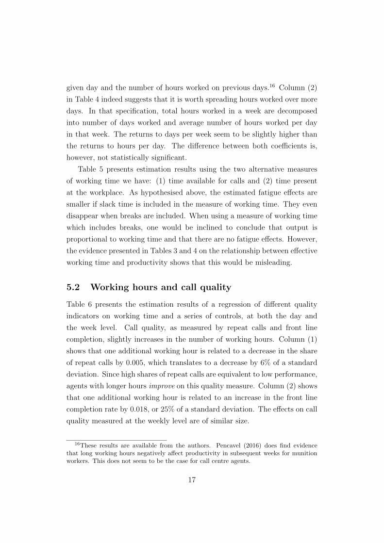
given day and the number of hours worked on previous days.16 Column (2)

in Table 4 indeed suggests that it is worth spreading hours worked over more

days. In that specification, total hours worked in a week are decomposed

into number of days worked and average number of hours worked per day

in that week. The returns to days per week seem to be slightly higher than

the returns to hours per day. The difference between both coefficients is,

however, not statistically significant.

Table 5 presents estimation results using the two alternative measures

of working time we have: (1) time available for calls and (2) time present

at the workplace. As hypothesised above, the estimated fatigue effects are

smaller if slack time is included in the measure of working time. They even

disappear when breaks are included. When using a measure of working time

which includes breaks, one would be inclined to conclude that output is

proportional to working time and that there are no fatigue effects. However,

the evidence presented in Tables 3 and 4 on the relationship between effective

working time and productivity shows that this would be misleading.

5.2 Working hours and call quality

Table 6 presents the estimation results of a regression of different quality

indicators on working time and a series of controls, at both the day and

the week level. Call quality, as measured by repeat calls and front line

completion, slightly increases in the number of working hours. Column (1)

shows that one additional working hour is related to a decrease in the share

of repeat calls by 0.005, which translates to a decrease by 6% of a standard

deviation. Since high shares of repeat calls are equivalent to low performance,

agents with longer hours improve on this quality measure. Column (2) shows

that one additional working hour is related to an increase in the front line

completion rate by 0.018, or 25% of a standard deviation. The effects on call

quality measured at the weekly level are of similar size.

16These results are available from the authors. Pencavel (2016) does find evidencethat long working hours negatively affect productivity in subsequent weeks for munitionworkers. This does not seem to be the case for call centre agents.

17

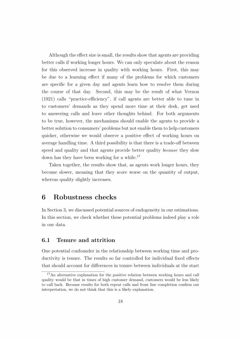
Although the effect size is small, the results show that agents are providing

better calls if working longer hours. We can only speculate about the reason

for this observed increase in quality with working hours. First, this may

be due to a learning effect if many of the problems for which customers

are specific for a given day and agents learn how to resolve them during

the course of that day. Second, this may be the result of what Vernon

(1921) calls “practice-efficiency”, if call agents are better able to tune in

to customers’ demands as they spend more time at their desk, get used

to answering calls and leave other thoughts behind. For both arguments

to be true, however, the mechanisms should enable the agents to provide a

better solution to consumers’ problems but not enable them to help customers

quicker, otherwise we would observe a positive effect of working hours on

average handling time. A third possibility is that there is a trade-off between

speed and quality and that agents provide better quality because they slow

down has they have been working for a while.17

Taken together, the results show that, as agents work longer hours, they

become slower, meaning that they score worse on the quantity of output,

whereas quality slightly increases.

6 Robustness checks

In Section 3, we discussed potential sources of endogeneity in our estimations.

In this section, we check whether these potential problems indeed play a role

in our data.

6.1 Tenure and attrition

One potential confounder in the relationship between working time and pro-

ductivity is tenure. The results so far controlled for individual fixed effects

that should account for differences in tenure between individuals at the start

17An alternative explanation for the positive relation between working hours and callquality would be that in times of high customer demand, customers would be less likelyto call back. Because results for both repeat calls and front line completion confirm ourinterpretation, we do not think that this is a likely explanation.

18

of the observation period. If, however, more productive agents have lower

turnover than less productive agents, high-productivity agents could be over-

represented in the sample. In this case, we may overestimate the returns to

hours, or underestimate the effects of fatigue.

To account for potential differences in how fast individuals learn on the

job, we estimate a model in which we control for an individual-specific time

trend (i.e. an interaction of the individual fixed effect with the time trend).

Table 7 presents the estimation results, both at the day and at the week

level. The individual-specific time trends typically have positive coefficients,

confirming the idea that individuals learn on the job. Controlling for a (daily

or weekly) time trend at the individual level does not affect the estimated

coefficient on hours worked much, compared to the results in Tables 3 and 4.

This suggests that differences in learning speed between individuals are not

an important confounder.18

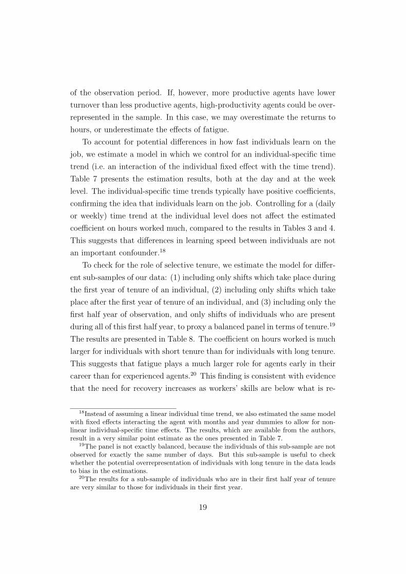
To check for the role of selective tenure, we estimate the model for differ-

ent sub-samples of our data: (1) including only shifts which take place during

the first year of tenure of an individual, (2) including only shifts which take

place after the first year of tenure of an individual, and (3) including only the

first half year of observation, and only shifts of individuals who are present

during all of this first half year, to proxy a balanced panel in terms of tenure.19

The results are presented in Table 8. The coefficient on hours worked is much

larger for individuals with short tenure than for individuals with long tenure.

This suggests that fatigue plays a much larger role for agents early in their

career than for experienced agents.20 This finding is consistent with evidence

that the need for recovery increases as workers’ skills are below what is re-

18Instead of assuming a linear individual time trend, we also estimated the same modelwith fixed effects interacting the agent with months and year dummies to allow for non-linear individual-specific time effects. The results, which are available from the authors,result in a very similar point estimate as the ones presented in Table 7.

19The panel is not exactly balanced, because the individuals of this sub-sample are notobserved for exactly the same number of days. But this sub-sample is useful to checkwhether the potential overrepresentation of individuals with long tenure in the data leadsto bias in the estimations.

20The results for a sub-sample of individuals who are in their first half year of tenureare very similar to those for individuals in their first year.

19

quired for their job (Gommans et al., 2016). If workers learn on the job, they

should be less subject to fatigue as they become more experienced. But the

finding of smaller fatigue effects for agents with longer tenure is also consis-

tent with the idea that tenure is selective, in the sense that agents who are

less subject to fatigue are more likely to remain in the call centre. In any

case, the effect of hours estimated in Table 3 actually covers heterogeneous

effects which depend on the tenure of an agent. Further, the coefficient on

hours obtained in Column (3) of Table 8 is very similar to the one obtained

in Table 3. As our results are similar whether we use a balanced panel or

not, attrition does not seem to be an important source of bias.

In estimations at the week level, we also observe a much stronger fatigue

effect for agents with less than a year tenure than for agents with more than

a year of experience. The fatigue effect even seems to be entirely driven

by individuals in their first year of tenure, and to disappear entirely for ex-

perienced agents at the week level. A possible explanation could be that

experienced agents are better able to recover from one day to another. Esti-

mation of a balanced panel yields results similar to those obtained in Table

4, suggesting that attrition does not bias the results.21

6.2 Scheduling as a source of exogeneity in hours worked

In Section 3, we argued that scheduling by the planning department of the call

centre ensures that the number of hours worked by an agent on a given day or

in a given week is exogenous. We also mentioned potential objections to this

argument: individuals can express schedule preferences for a specific day or

week, and they may be asked to stay shorter or longer in case of unforeseen

changes in the number of incoming calls. We address these objections here.

In Table 9, we estimate our preferred models at the day and week level,

including additional controls for the number of hours scheduled (Columns

(1) and (3)) or the deviation from the number of hours scheduled, defined as

21Results available from the authors. For individuals in their first year of tenure andfor the balanced sample, the results described here are only found after the week fixedeffects and the time trend are dropped out of the model. Estimation of the model withthe full set of controls seems to be hampered as the number of observations is reduced.

20

the difference between actual hours worked and scheduled hours for a week

(Columns (2) and (4)).22

The positive coefficient on hours scheduled in Columns (1) and (3) of

Table 9 suggests that individuals are indeed more (less) productive in weeks

for which their expressed preferences ensured that they were scheduled for

longer (shorter) hours. However, controlling for the length of schedules does

not lead to important changes in the estimated magnitudes of the coefficients

on working time. They are only slightly more negative, hinting at a slight

underestimation of the fatigue effect due to selective scheduling.

The results in Columns (2) and (4) show that hours worked on top of

scheduled hours are negatively related to productivity. It suggests that fa-

tigue becomes even stronger if the effort to be made by agents is unexpected.

This is intuitive, and is evidence against self-selection of agents in the sense

that they would volunteer to work more hours on days on which they are

more productive. The coefficient on working time becomes slightly less neg-

ative in this specification, which is logical because the total fatigue effect (as

estimated in Tables 3 and 4) is now decomposed into “simple” fatigue due to

working more hours and additional fatigue during unexpected extra hours.

All in all, the evidence presented in Table 9 suggests that self-selection by

agents is not an important source of bias in our estimations. Rather, it seems

plausible that scheduling exogenously determines the hours actually worked

by agents.

7 Conclusions

In this paper, we have estimated the impact of working time on productivity,

both at the daily and at the weekly level. We have used panel data on indi-

vidual workers of a call centre in the Netherlands, which contain information

about the number of hours worked, the number of calls answered, the average

22The number of observations drops because information about scheduled hours is notavailable for every agent. If we limit the estimation sample to agents with strictly positivescheduled hours, the results remain very similar, only the coefficient on scheduled hoursbecomes smaller. If we take up the log scheduled hours and log deviation in the modelsinstead of scheduled hours and deviation, the results remain virtually unchanged.

21

handling time of calls and indicators of call quality for every day worked by

an agent from mid-2008 until the first week of 2010. The panel character of

the data enables us to control for time-invariant unobserved heterogeneity.

Scheduling by the firm generates variation in the daily and weekly hours of

individual workers which is hardly related to individual time-varying char-

acteristics, since expected consumer demand is leading in making schedules.

This yields estimates of the effect of working time on productivity that are

not biased by individual shocks.

Our results show that an increase in effective working time by 1 percent

leads to an increase in output, i.e. the number of calls answered, by about

0.9 percent. This corresponds to moderately decreasing returns to hours,

probably due to fatigue among agents. Given that agents in our sample

work on average 4.6 effective hours per day, this shows that the call centre

environment is demanding and that fatigue sets in early. The fatigue effects

would be larger if the call agents worked full-time. This study complements

the small number of studies which examine the effect of working time on

productivity using an arguably exogenous source of variation in working time

(Crocker and Horst, 1981; Brachet et al., 2012; Pencavel, 2015; Dolton et al.,

2016), by providing evidence for medium-skilled jobs in the service sector.

As we are able to isolate effective working time and concentrate on this

measure, our estimates form an upper bound for the fatigue effect. Our

finding of decreasing returns to hours seems to hold best for individuals with

shorter tenure, while we find much less evidence of fatigue effects among more

experienced agents. Various indicators of call quality show that call quality

does not suffer as the number of hours worked increase. On the contrary, call

quality seems to slightly improve.

Our findings are most relevant for part-time medium-skilled jobs in the

service sector. They suggest that increasing the effective working time in

these occupations would cause individual workers, in particular the relatively

inexperienced ones, to produce smaller quantities of output per hour, due to

fatigue. Such an increase in working time could, however, be beneficial for

the quality provided. These findings are informative for firm management

and for working time regulation policies. The total economic effects of such

22

policies, however, are dependent not only on the effect of working hours on

labour productivity at the individual level, but also on many more factors

such as work organisation and availability of qualified workers.

References

Anxo, D. and A. Bigsten (1989): “Working Hours and Productivity in

Swedish Manufacturing,” Scandinavian Journal of Economics, 91, 613–

619.

Bakker, A., E. Demerouti, and W. Schaufeli (2003): “Dual processes

at work in a call centre: An application of the job demands–resources

model,” European Journal of work and organizational psychology, 12, 393–

417.

Barzel, Y. (1973): “The Determination of Daily Hours and Wages,” The

Quarterly Journal of Economics, 87, 220–238.

Bick, A., B. Bruggemann, and N. Fuchs-Schundeln (2016): “Hours

Worked in Europe and the US: New Data, New Answers,” IZA Discussion

Papers 10179, Institute for the Study of Labor (IZA).

Brachet, T., G. David, and A. M. Drechsler (2012): “The Effect

of Shift Structure on Performance,” American Economic Journal: Applied

Economics, 4, 219–246.

Breuer, K., P. Nieken, and D. Sliwka (2013): “Social ties and sub-

jective performance evaluations: an empirical investigation,” Review of

managerial Science, 7, 141–157.

Craine, R. (1973): “On the Service Flow from Labour,” Review of Eco-

nomic Studies, 40, 39–46.

23

Crepon, B., M. Leclair, and S. Roux (2004): “RTT, productivite

et emploi: nouvelles estimations sur donnees d’entreprises,” Economie et

statistique, 376, 55–89.

Crocker, T. D. and R. L. Horst (1981): “Hours of Work, Labor Pro-

ductivity, and Environmental Conditions: A Case Study,” Review of Eco-

nomics and Statistics, 63, 361–368.

De Grip, A. and J. Sauermann (2012): “The Effects of Training on

Own and Co-worker Productivity: Evidence from a Field Experiment,”

Economic Journal, 122, 376–399.

De Grip, A., J. Sauermann, and I. Sieben (2016): “Tenure-

Performance Profiles and the Role of Peers: Evidence from Personnel

Data,” Journal of Economic Behavior & Organization, 126, 679–695.

DeBeaumont, R. and L. D. Singell (1999): “The Return to Hours and

Workers in U. S. Manufacturing: Evidence on Aggregation Bias,” Southern

Economic Journal, 66, 336–352.

Devicienti, F., E. Grinza, and D. Vannoni (2015): “The Impact of

Part-Time Work on Firm Total Factor Productivity: Evidence from Italy,”

IZA Discussion Papers 9463, Institute for the Study of Labor (IZA).

Dolton, P., C. Howorth, and M. Abouaziza (2016): “The Optimal

Length of the Working Day: Evidence from Hawthorne Experiments,”

ESPE conference paper.

Feldstein, M. S. (1967): “Specification of the labour input in the aggregate

production function,” Review of Economic Studies, 34, 375–386.

Garnero, A., S. Kampelmann, and F. Rycx (2014): “Part-Time Work,

Wages, and Productivity Evidence from Belgian Matched Panel Data,”

Industrial & Labor Relations Review, 67, 926–954.

Gianella, C. and P. Lagarde (2011): “Productivity of hours in the

aggregate production function: An evaluation on a panel of French firms

from the manufacturing sector,” Tech. rep., Insee.

24

Goldmark, J. (1912): Fatigue and Efficiency: A Study in Industry, New

York: Russel Sage.

Gommans, F., N. Jansen, D. Stynen, I. Kant, and A. de Grip

(2016): “The impact of underskilling on need for recovery, losing employ-

ment and retirement intentions among older office workers: A prospective

cohort study,” International Labour Review, forthcoming.

Hart, A. and S. Krall (2007): “220: Productivity: Do 8-9 Hour Shifts

Make a Difference?” Annals of Emergency Medicine, 50, S69–S70.

Hart, R. A. and P. G. McGregor (1988): “The returns to labour

services in West German manufacturing industry,” European Economic

Review, 32, 947–963.

Ilmakunnas, P. (1994): “Returns to workers and hours in Finnish manu-

facturing,” Empirical Economics, 19, 533–553.

Kodz, J., S. Davis, D. Lain, M. Strebler, J. Rick, P. Bates,

J. Cummings, N. Meager, D. Anxo, S. Gineste, et al. (2003):

“Working long hours: A review of the evidence. Volume 1–Main report,”

Employment Relations Research Series, 16.

Kossoris, M. D. (1947): “Hours of work and output,” Monthly Labor Re-

view, 65, 5.

Kramarz, F., P. Cahuc, B. Crepon, T. Schank, O. N. Skans,

G. van Lomwel, and A. Zylberberg (2008): “Labour market ef-

fects of work-sharing arrangements in Europe,” in Working hours and job

sharing in the EU and USA: Are Europeans lazy? Or Americans crazy?,

ed. by T. Boeri, M. Burda, and F. Kramarz, Oxford University Press,

171–196.

Kunn-Nelen, A., A. De Grip, and D. Fouarge (2013): “Is part-time

employment beneficial for firm productivity?” Industrial & Labor Rela-

tions Review, 66, 1172–1191.

25

Lee, J. and Y.-K. Lee (2016): “Can working hour reduction save work-

ers?” Labour Economics, 40, 25–36.

Leslie, D. (1984): “The Productivity of Hours in U.S. Manufacturing In-

dustries,” Review of Economics and Statistics, 66, 486–490.

Leslie, D. and J. Wise (1980): “The Productivity of Hours in U.K. Man-

ufacturing and Production Industries,” Economic Journal, 90, 74–84.

Liu, X. and R. Batt (2007): “The economic pay-offs to informal training:

evidence from routine service work,” Industrial & Labor Relations Review,

61, 75–89.

Lu, S. F. and L. X. Lu (2016): “Do Mandatory Overtime Laws Im-

prove Quality? Staffing Decisions and Operational Flexibility of Nursing

Homes,” Management Science, forthcoming.

McClay, J. (2008): “357: Comparison of Ten-Hour and Twelve-Hour Shifts

Demonstrates No Difference in Resident Productivity,” Annals of Emer-

gency Medicine, 52, S151.

Nyland, C. (1989): Reduced worktime and the management of production,

Cambridge: Cambridge University Press.

OECD (2016): OECD Employment Outlook 2016, OECD Publishing.

Pencavel, J. (2015): “The Productivity of Working Hours,” Economic

Journal, 125, 2052–2076.

——— (2016): “Recovery from Work and the Productivity of Working

Hours,” Economica, 83, 545–563.

Rogers, A. E., W.-T. Hwang, L. D. Scott, L. H. Aiken, and D. F.

Dinges (2004): “The working hours of hospital staff nurses and patient

safety,” Health Affairs, 23, 202–212.

Schank, T. (2005): “Are overtime plants more efficient than standard-time

plants? A stochastic production frontier analysis using the IAB Establish-

ment Panel,” Empirical Economics, 30, 693–710.

26

Shepard, E. and T. Clifton (2000): “Are longer hours reducing produc-

tivity in manufacturing?” International Journal of Manpower, 21, 540–

553.

Specchia, G. and V. Vandenberghe (2013): “Is Part-time Employment

a Boon or Bane for Firm Productivity?” Tech. rep., IRES Working Paper.

Tatom, J. A. (1980): “The “Problem” of procyclical real wages and pro-

ductivity,” Journal of Political Economy, 88, 385–394.

van der Hulst, M. (2003): “Long workhours and health,” Scandinavian

Journal of Work, Environment & Health, 29, 171–188.

van Dijk, F. J. H. and G. M. H. Swaen (2003): “Fatigue at work,”

Occupational and Environmental Medicine, 60, i1–i2.

Vegso, S., L. Cantley, M. Slade, O. Taiwo, K. Sircar, P. Rabi-

nowitz, M. Fiellin, M. Russi, and M. Cullen (2007): “Extended

work hours and risk of acute occupational injury: A case-crossover study

of workers in manufacturing,” American Journal of Industrial Medicine,

50, 597–603.

Vernon, H. M. (1921): Industrial fatigue and efficiency, London: Rout-

ledge & Sons.

27

Figures

Figure 1: Density of daily productivity0

.002

.004

.006

Den

sity

0 200 400 600 800 1000Average handling time (in seconds)

Note: The figure shows how the density plot of daily productivity, as measured by the average handling

time (in seconds).

Figure 2: Productivity by working hours

(a) Descriptive results

0.0

05.0

1.0

15Pr

oduc

tivity

(1/A

HT)

0 2 4 6 8Daily working hours

(b) Estimation results

-.001

0.0

01.0

02.0

03Ef

fect

on

prod

uctiv

ity (1

/AH

T)

0 2 4 6 8Daily working hours

Note: Panel (a) shows average productivity over working time for 15-minute intervals. The capped spikes

present the corresponding 5th and 95th percentile of the productivity distribution. Panel (b) shows the

coefficients on dummies for 15-minute working time intervals in a regression as in model (7) from Table

3. The capped spikes present the corresponding 95-percent confidence intervals. The reference category

is 21 quarters of an hour, i.e. 5 hours and 15 minutes.

28

Tables

Table 1: Descriptive statistics

Variable Mean Std. Dev. Min. Max. NDay levelAverage handling time (AHT) 321.613 111.012 3 910.364 33,123Productivity (1/AHT) 0.004 0.003 0.001 0.333 33,123Calls Answered 55.795 22.992 1 129 33,123Daily working hours 4.621 1.516 0.001 7.747 33,123Starting time 11.445 3.079 1 24 33,120Share of repeat calls 0.164 0.084 0 1 33,123Front line completion rate 0.956 0.072 0 1 32,831Working hours 4.621 1.516 0.001 7.747 33,123Hours available for calls 4.812 1.414 0.001 7.903 33,123Hours present at the workplace 6.05 1.476 0.01 9.52 33,123Week levelAverage handling time (AHT) 319.314 100.133 5 910.364 8,641Productivity (1/AHT) 0.003 0.002 0.001 0.2 8,641Calls answered 213.876 114.138 1 645 8,641Weekly working hours 17.712 8.458 0.001 43.046 8,641Days per week 4.020 1.282 1 7 8,641Tenure in weeks 149.58 191.623 1 691 8,587Share of repeat calls over week 0.167 0.066 0 1 8,641Front line completion rate over week 0.950 0.083 0 1 8,641Working hours 17.712 8.458 0.001 43.046 8,641Hours available for calls 18.447 8.334 0.001 42.929 8,641Hours present at the workplace 23.191 9.775 0.02 50.56 8,641Hours scheduled for the week 19.805 9.573 0 51 6,513Agent levelN of agents 332Male 0.351 0.478 0 1 305Age 29.542 10.578 17 65 284

29

Table 2: Variation in daily and weekly working hours

Day level:Working hoursh (rounded at 1)

Observations withh hours

Individuals with hhours at least once

Conditional on working h hoursat least once, share of days inwhich individual works h hours

0 473 135 2.741 1211 192 6.132 1663 215 6.493 3228 276 11.14 5325 315 17.45 14372 317 45.846 3461 275 12.567 3211 202 17.248 179 70 3.51Total 33,123Week level:Working hours h(rounded at 4)

Observations withh hours

Individuals with hhours at least once

Conditional on working h hoursat least once, share of weeks inwhich individual works h hours

0 187 92 7.254 725 227 13.68 997 224 17.212 1124 245 15.4616 1262 247 17.6820 1229 249 20.3724 1621 232 27.0228 968 189 19.9532 350 114 13.136 171 66 11.7840 6 6 8.1144 1 1 9.09Total 8,641

30

Table 3: Relationship between productivity and working time at the day level

(1) (2) (3) (4) (5) (6) (7) (8)Log working hours -0.175*** -0.152*** -0.151*** -0.151*** -0.137*** -0.128*** -0.113*** -0.139***

(0.007) (0.013) (0.013) (0.013) (0.013) (0.012) (0.013) (0.011)Trend 0.001*** 0.001*** 0.001*** 0.001*** 0.001*** 0.001***

(0.000) (0.000) (0.000) (0.000) (0.000) (0.000)Day of the week dummies (reference: Monday)Tuesday 0.004 0.007* -0.023 -0.452***

(0.004) (0.003) (0.024) (0.045)Wednesday -0.000 0.001 0.029 -0.427***

(0.004) (0.004) (0.025) (0.052)Thursday -0.001 0.001 0.066*** -0.609***

(0.004) (0.003) (0.025) (0.063)Friday 0.004 0.006* 0.011 -0.424***

(0.004) (0.004) (0.026) (0.050)Saturday 0.109*** 0.110*** -0.471*** -0.890***

(0.008) (0.007) (0.069) (0.074)Sunday 0.809*** 0.417*** 0.806*** 0.608***

(0.058) (0.063) (0.039) (0.040)Age -0.001***

(0.000)Tenure 0.008***

(0.000)Male -0.003

(0.004)Individual fixed effects No Yes Yes Yes Yes Yes Yes NoTeam fixed effects No No No Yes Yes Yes Yes YesHour-of-the-day dummies No No No No No Yes Yes YesDay fixed effects No No No No No No Yes YesR-squared 0.085 0.094 0.152 0.160 0.198 0.285 0.385 0.403N 33,123 33,123 33,123 33,123 33,123 33,123 33,123 31,525Individuals 332 332 332 332 332 332 332

Note: * p< 0.10; ** p< 0.05; *** p< 0.01; ordinary least squares regression; dependent variable =ln(1/AHT ); robust standard errors in parentheses.

31

Table 4: Relationship between productivity and working time at the weeklevel

(1) (2)Log weekly working hours -0.078**

(0.031)Log days per week -0.066**

(0.032)Log average hours per day -0.079**

(0.031)Trend (weekly) 0.004*** 0.004***

(0.001) (0.001)R-squared 0.345 0.345N 8,641 8,641Individuals 332 332

Note: * p< 0.10; ** p< 0.05; *** p< 0.01; ordinary least squares regression; dependent variable =ln(1/AHT ); robust standard errors in parentheses. All regressions include agent, week, and team fixedeffects. The regressions also include hour-of-the-week fixed effects, which are defined as 168 dummies foreach hour of the week during which an individual works.

Table 5: Alternative working time definitions and the relationship betweenproductivity and working time

(1) (2) (3) (4)Day level Week level

Log daily hours available for calls -0.078***(0.015)

Log daily hours present at the workplace -0.016(0.015)

Trend (daily) 0.001*** 0.001***(0.000) (0.000)

Log weekly hours available for calls -0.050(0.035)

Log weekly hours present at the workplace -0.020(0.029)

Trend (weekly) 0.004*** 0.004***(0.001) (0.001)

R-squared 0.368 0.357 0.335 0.329N 33,123 33,123 8,641 8,641Individuals 332 332 332 332

Note: * p< 0.10; ** p< 0.05; *** p< 0.01; ordinary least squares regression; dependent variable =ln(1/AHT ); robust standard errors in parentheses. All regressions include agent and team fixed effects.Regressions at the day level include day fixed effects, hour-of-the-day fixed effects and day-of-the-weekfixed effects. Regressions at the week level include week fixed effects and hour-of-the-week fixed effects.Day-of-the-week (hour-of-the-week) fixed effects are defined as dummies for each hour of the day (week)an individual works.

32

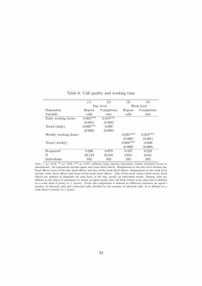
Table 6: Call quality and working time

(1) (2) (3) (4)Day level Week level

Dependent Repeat Completion Repeat CompletionVariable calls rate calls rateDaily working hours -0.005*** 0.018***

(0.001) (0.002)Trend (daily) 0.000*** 0.000

(0.000) (0.000)Weekly working hours -0.001*** 0.012***

(0.000) (0.001)Trend (weekly) 0.002*** -0.000

(0.000) (0.000)R-squared 0.200 0.079 0.237 0.223N 33,123 32,831 8,641 8,641Individuals 332 332 332 332

Note: * p< 0.10; ** p< 0.05; *** p< 0.01; ordinary least squares regression; robust standard errors inparentheses. All regressions include agent and team fixed effects. Regressions at the day level include dayfixed effects, hour-of-the-day fixed effects and day-of-the-week fixed effects. Regressions at the week levelinclude week fixed effects and hour-of-the-week fixed effects. Day-of-the-week (hour-of-the-week) fixedeffects are defined as dummies for each hour of the day (week) an individual works. Repeat calls aredefined as the share of customers to whom an agent spoke who call back within seven days and is definedon a scale from 0 (best) to 1 (worst). Front line completion is defined as difference between an agent’snumber of inbound calls and outbound calls, divided by the number of inbound calls. It is defined on ascale from 0 (worst) to 1 (best).

33

Table 7: Individual-specific time trends and the relationship between pro-ductivity and working time

(1) (2)Day level Week level

Log daily working hours -0.104***(0.013)

Trend (daily) -0.000***(0.000)

Log weekly working hours -0.071**(0.034)

Trend (weekly) -0.001*(0.001)

Agent-specific day trend Yes NoAgent-specific week trend No YesR-squared 0.479 0.496N 33,123 8,641Individuals 332 332

Note: * p< 0.10; ** p< 0.05; *** p< 0.01; ordinary least squares regression; dependent variable =ln(1/AHT ); robust standard errors in parentheses. All regressions team fixed effects. Regressions atthe day level include day fixed effects, hour-of-the-day fixed effects and day-of-the-week fixed effects.Regressions at the week level include week fixed effects and hour-of-the-week fixed effects. Day-of-the-week (hour-of-the-week) fixed effects are defined as dummies for each hour of the day (week) an individualworks.

Table 8: Tenure, attrition, and the relationship between productivity andworking time at the day level

(1) (2) (3)Log daily working hours -0.141*** -0.078*** -0.100***

(0.022) (0.014) (0.023)Trend (daily) 0.002*** 0.000*** -0.000

(0.000) (0.000) (0.000)R-squared 0.421 0.430 0.499N 15,664 17,326 9,366Individuals 249 131 104

Note: * p< 0.10; ** p< 0.05; *** p< 0.01; ordinary least squares regression; sample is restricted toindividuals with a year tenure or less (Column (1)), with more than a year tenure (Column (2)), and onlythe first half year of observation and only shifts of individuals who are present during all of this first halfyear (Column (3)); robust standard errors in parentheses. All regressions include agent, day fixed effectsand team fixed effects. Regressions also include hour-of-the-day fixed effects and day-of-the-week fixedeffects, which are defined as dummies for each hour of the day and day of the week an individual works.

34

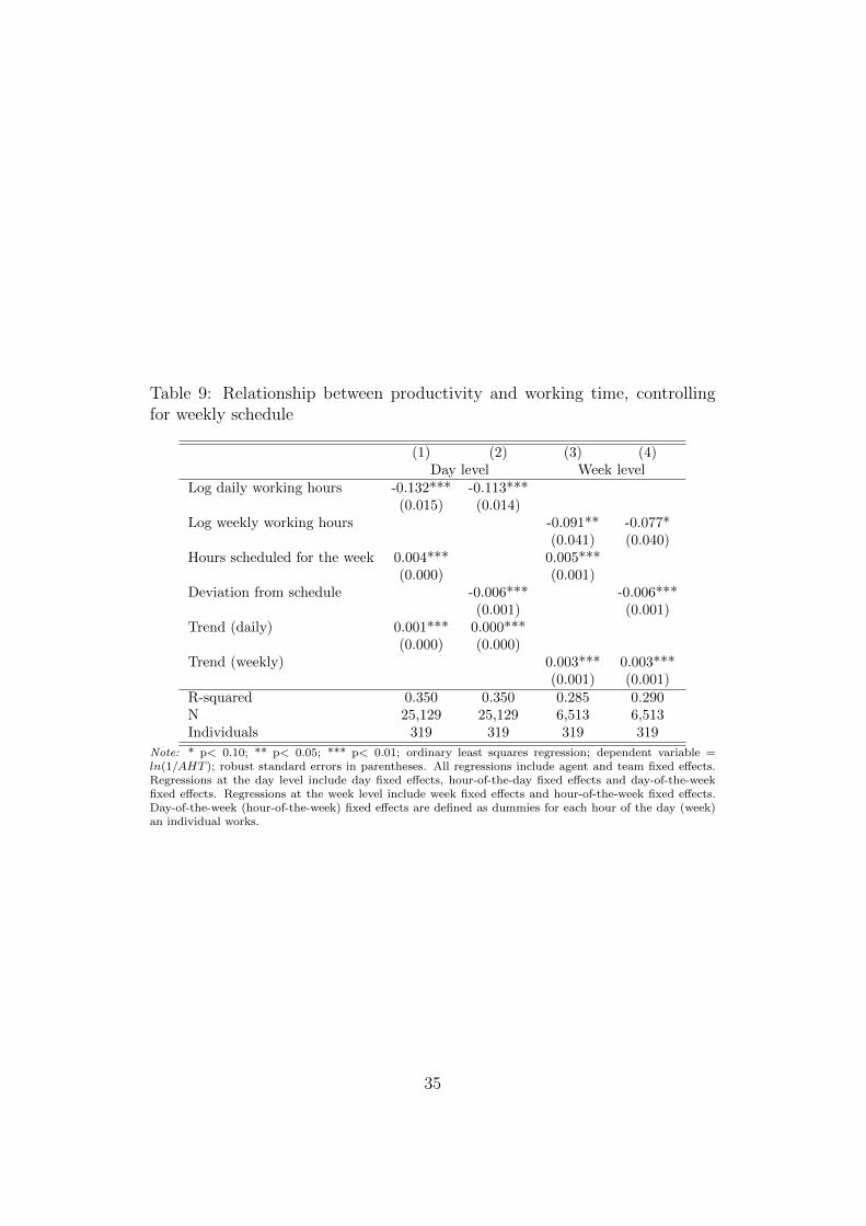
Table 9: Relationship between productivity and working time, controllingfor weekly schedule

(1) (2) (3) (4)Day level Week level

Log daily working hours -0.132*** -0.113***(0.015) (0.014)

Log weekly working hours -0.091** -0.077*(0.041) (0.040)

Hours scheduled for the week 0.004*** 0.005***(0.000) (0.001)

Deviation from schedule -0.006*** -0.006***(0.001) (0.001)

Trend (daily) 0.001*** 0.000***(0.000) (0.000)

Trend (weekly) 0.003*** 0.003***(0.001) (0.001)

R-squared 0.350 0.350 0.285 0.290N 25,129 25,129 6,513 6,513Individuals 319 319 319 319

Note: * p< 0.10; ** p< 0.05; *** p< 0.01; ordinary least squares regression; dependent variable =ln(1/AHT ); robust standard errors in parentheses. All regressions include agent and team fixed effects.Regressions at the day level include day fixed effects, hour-of-the-day fixed effects and day-of-the-weekfixed effects. Regressions at the week level include week fixed effects and hour-of-the-week fixed effects.Day-of-the-week (hour-of-the-week) fixed effects are defined as dummies for each hour of the day (week)an individual works.

35