DISCUSSION PAPER SERIES

IZA DP No. 10800

Péter ElekJános Köllő

Eliciting Permanent and Transitory Undeclared Work from Matched Administrative and Survey Data

MAY 2017

Any opinions expressed in this paper are those of the author(s) and not those of IZA. Research published in this series may include views on policy, but IZA takes no institutional policy positions. The IZA research network is committed to the IZA Guiding Principles of Research Integrity.The IZA Institute of Labor Economics is an independent economic research institute that conducts research in labor economics and offers evidence-based policy advice on labor market issues. Supported by the Deutsche Post Foundation, IZA runs the world’s largest network of economists, whose research aims to provide answers to the global labor market challenges of our time. Our key objective is to build bridges between academic research, policymakers and society.IZA Discussion Papers often represent preliminary work and are circulated to encourage discussion. Citation of such a paper should account for its provisional character. A revised version may be available directly from the author.

Schaumburg-Lippe-Straße 5–953113 Bonn, Germany

Phone: +49-228-3894-0Email: publications@iza.org www.iza.org

IZA – Institute of Labor Economics

DISCUSSION PAPER SERIES

IZA DP No. 10800

Eliciting Permanent and Transitory Undeclared Work from Matched Administrative and Survey Data

MAY 2017

Péter ElekEötvös Loránd University (ELTE)

János KöllőHungarian Academy of Sciences and IZA

ABSTRACT

MAY 2017IZA DP No. 10800

Eliciting Permanent and Transitory Undeclared Work from Matched Administrative and Survey Data*

We study the undeclared work patterns of Hungarian employees in relatively stable jobs,

using a panel dataset that matches individual-level self-reported Labour Force Survey

data with administrative records of the Pension Directorate for 2001–2006. We estimate

the determinants of undeclared work using Heckman-type random-effects panel probit

models, and develop a two-regime model to separate permanent and transitory undeclared

work, where the latter follows a Markov chain. We find that about 6-7 per cent of workers

went permanently unreported for six consecutive years, and a further 4 per cent were

transitorily unreported in any given year. The models show lower reporting rates – especially

in the permanent segment – among males, high-school graduates, those in agriculture and

transport, various forms of atypical employment, and small firms. Transitory non-reporting

may be partly explained by administrative records missing for technical reasons. The results

suggest that (i) the ‘aggregate labour input method’ widely used in Europe can indeed be

a simple yet reliable tool to estimate the size of informal employment, although it slightly

overestimates the true magnitude of black work (ii) the long-term pension consequences

of undeclared work are substantial because of the high share of permanent non-reporting.

JEL Classification: C23, C25, H26, J46

Keywords: undeclared work, labour input method, matched administrative-survey data, random-effects panel probit with endogenous selection, Markov chain

Corresponding author:János KöllőInstitute of EconomicsHungarian Academy of SciencesH-1112 BudapestBudaörsi út 45Hungary

E-mail: kollo. janos@krtk.mta.hu

* The authors would like to thank Anikó Bíró, Márton Csillag and Gábor Kézdi for useful comments on an earlier version of the paper. Péter Elek was supported by the János Bolyai Research Scholarship of the Hungarian Academy of Sciences.

2

1. Introduction

Undeclared employment – when the worker is not reported to the authorities and neither

the employer nor the employee pay taxes or contributions in the relationship – is

notoriously difficult to measure. Survey-based methods rely on information directly

provided by the population, but these tend to underestimate the true magnitude of black

work, and are strongly affected by cultural differences. For instance, according to the

Eurobarometer Survey, only 4 per cent of the EU population responded in 2013 that they

had undertaken undeclared paid work in the preceding year (European Commission,

2014); the highest rates were recorded in Latvia, the Netherlands, Estonia and Denmark

(9–11 per cent), while Southern European countries reported very low rates (1–3 per cent

in Malta, Portugal, Cyprus, Italy and Greece).

Indirect methods estimate total employment with observable proxies, and compare these

with reported employment figures to obtain a measure of undeclared work. A wide range

of techniques fall into this category,1 the most promising being the discrepancy or labour

input method, which was advocated by a task force as a methodologically appropriate

tool for EU-wide measurement of undeclared work (GHK/FGB, 2009). This technique

assumes that labour force surveys register most of the undeclared work because

individuals are not motivated to conceal their true employment status in an unofficial

interview. Hence undeclared work can be approximated by comparing Labour Force

Survey (LFS) employment with registered employment figures, which may come from

administrative sources or enterprise surveys. This method – in line with other indirect

techniques (Schneider, 2012) – yields considerably larger estimates of undeclared work

1 Examples are the consumption-income discrepancy method, the monetary method, the electricity

consumption method and econometric methods such as MIMIC (Renooy et al., 2004; Schneider, 2012).

3

than do survey-based methods: e.g. 16–17 per cent of total employment in Hungary

between 2001 and 2005 (Elek et al., 2009; Benedek et al., 2013) and 8–30 per cent of

various macroeconomic aggregates in European countries.2 These estimates do not suffer

from the underreporting bias of surveys, but they are generally not suitable for

multivariate analysis, because only group-wise comparisons are possible, across

dimensions that are available in both data sources. Hence, most analysis using the labour

input method provides only sectoral, regional or gender-specific breakdown (GHK/FGB,

2009).

In this paper, we exploit a unique panel dataset from Hungary that matches self-reported

and administrative employment data at the individual level. The data relate to workers

who reported at least two years of uninterrupted tenure in the jobs they held in January–

March 2008, when they were interviewed for the LFS. We assess the pensionable years

they accrued in 2001–2006, using quality-checked administrative data provided by the

National Pension Insurance Directorate (NPID). The matched data enable us to combine

the strengths of the ‘labour input’ method and survey-based methods by analysing the

determinants of undeclared work in a multivariate setting. We examine the data with

regard to biases stemming from non-random sampling, recall bias on the part of LFS

respondents, and technical failures and negligence on the part of employers, the NPID or

the postal service. Methodologically, we estimate random-effects (RE) linear and probit

models as well as a RE probit model with endogenous selection to account for non-

2 For instance, 11.5 per cent of employment in full-time equivalent units for Italy in 2004 (Baldassarini,

2007), 17–21 per cent of official GDP for Slovenia between 1995 and 2004 (Nastav and Bojnec, 2007),

8 per cent of total employment for Spain in 2002 and 20–30 per cent of GDP for Romania between 1996

and 2002 (for these and other EU country results, see GHK/FGB, 2009, pp. 49 and 77).

4

random sampling in the matched panel dataset. These models are estimated with

maximum simulated likelihood.

As a further advantage, the dataset allows us to separate permanent and transitory non-

reporting. We build a two-regime model, where both permanent and transitory non-

reporting probabilities depend on the observables through probit link functions, and

where transitory non-reporting follows a Markov chain. This model is estimated with

maximum likelihood.

We find that of those workers who were observed in the sample for six years, around 6–

7 per cent were never reported; around 3-4 per cent were unreported only once; and

around 4 per cent were unreported between two and five times. The econometric estimates

(especially those relating to permanently unreported workers) offer support for the

hypothesis that the bulk of non-reporting reflects informal employment: in line with other

studies, they predict lower reporting rates in, for example, agriculture and transport,

various forms of atypical work, among males and in small firms.

The two-regime model allows us to examine the consequences of undeclared work on

access to health care and pensions. We estimate that about one in ten workers are at risk

of receiving only emergency treatment in health care, and about 6 per cent foresee a

substantial loss (of 15 per cent or more) in terms of old-age pensions.

Our analysis relates to two strands of existing literature. According to the traditional

economic approach (Slemrod and Yitzhaki, 2002), economic actors make decisions about

tax evasion by comparing expected fines and the amount of tax that can be evaded.

Therefore, tax evasion is reduced by higher individual risk aversion, stronger deterrence

and lower tax rates (Buehn and Schneider, 2012). However, it is difficult to explain

5

willingness to pay taxes using the standard economic model – considering the limited risk

of being caught and the rates of potential fines – and therefore more recent literature

incorporates the effect of the social environment, such as rule following, the need to

belong to groups and other interactions (Feld and Larsen, 2012; Pickhardt and Prinz,

2014). The monopsonistic position of employers and the low bargaining power of

employees may also be important (Cichocki and Tyrowicz, 2010). Our estimates of

differences in undeclared work across gender, level of education, work experience,

occupation, place of residence, sector, size and ownership of the employer provide insight

into how differences in risk aversion, the expected costs of cheating and social

interactions influence the prevalence of undeclared work. These results complement

already existing cross-sectional multivariate analyses of undeclared work, which are,

however, mainly available from survey-based studies (Williams, 2007; Feld and Larsen,

2012; European Commission, 2014).

By giving a detailed description of the dynamics of non-reporting, our approach is also

related to the literature that models measurement error in earnings using matched

administrative and survey data (Pischke, 1995; Abowd and Stinson, 2013). A few papers

focus specifically on tax evasion using matched microdata (Baldini et al., 2009; Paulus,

2015). However, in contrast to our paper, that stream of literature does not concentrate on

undeclared work (i.e. full income tax evasion) and also follows a different econometrics

modelling framework, because earnings are continuous, whereas our undeclared work

dummy is a binary variable.

6

2. Data and descriptive analysis

2.1. Data

As was already mentioned, in January–March 2008, LFS respondents were offered the

chance to obtain precise information about their registered accrual years, and were asked

in return to permit the NPID and the Hungarian Central Statistical Office to use their

merged data for research purposes. The dataset created in this way contains all variables

of the LFS wave and the respondents’ annual reported days in work since their first

appearance in the NPID register.

Our key variable measures reported days in each full year that the respondent spent with

the employer. Registered days within a full year can vary between zero and 365 (or 366),

since holidays and paid leave are counted as insured periods. We would expect 100 per

cent of the time that workers spent with their employers to appear in the NPID register,

and so we can interpret the difference between reported and total days as a measure of

unregistered work.

However, our key measure is subject to biases for at least three reasons: (i) the sample is

non-random; (ii) employment spells perceived by the LFS respondents as continuous may

not be regarded as continuous by the NPID; and (iii) some NPID records may be missing

for technical reasons (unsent or lost).

Dealing with non-random selection. Of the 31,195 LFS respondents over 15 years of age

and not in receipt of a pension in 2008, some 7,654 (25 per cent) requested information

from the NPID (of these, 4,707 were employed according to the LFS). The incentive

7

offered – for an individual to acquire her official employment history – was likely to be

related to the time spent undeclared; hence the matched sample is non-random.3

We allow for self-selection in two ways. First, we use observables to estimate the

probability (p) that an LFS respondent requested information from the NPID (see the

selection equation later in Section 3.2 and the results in Table 5) and apply 1/p to give a

reweighted estimate of aggregate non-reporting. Statistics with and without weighting

suggest that the results are weakly affected by the weighting scheme. For instance,

unreported days accounted for 9.5 per cent in the unweighted and 10.4 per cent in the

weighted sample on average.4

Second, and more importantly, selection to the LFS–NPID sample could potentially be

affected by unobservables that also influence the probability of undeclared work. To

tackle this problem, we use an instrumental variable that is correlated with the probability

of being in the sample, but is uncorrelated with registration history. We discuss this in

detail in Section 3.2.

Unreported work versus temporary breaks. The share of declared working days during a

permanent-looking employment spell may fall short of the expected 100 per cent for

reasons other than non-reporting. Seasonal slumps, stoppages, strikes, unpaid leave and

absenteeism may cause breaks in the spell of employment, without dissolution of the

employment relationship. Thanks to retrospective questions in the LFS, we are in a

position to measure the incidence of such ‘real’ breaks with some precision.

3 Hungarians typically have no precise information on their accumulated accrual points and expected

pensions before they actually retire. The computer records (since 1988) and printed material that records

registered workdays and contribution payments are available to individuals before their retirement only

after a lengthy administrative procedure. 4 Similar small differences occur if the data are reweighted according to the LFS weights that are supplied

by the Central Statistical Office to correct for non-response in the LFS. In the following we will use the

unweighted data unless stated otherwise. For further details, see Bálint et al. (2010).

8

The event of interest is non-employment (by LFS standards) during an LFS-reported

employment relationship. For the study of such events, we selected employed workers

from the 2001–2006 waves of the LFS, who had entered their jobs more than 12 months

before the LFS interview and counted those who said that exactly 12 months before the

interview they had not been working. We found that only a tiny minority – around 1.5 per

cent – of those in permanent employment reported breaks in work. These figures,

compared to 9.5–10.4 per cent missing from the NPID register, suggest that the difference

between LFS-reported and registered employment stems primarily from underreporting.

Accounting for administrative failure. Unsent and lost reports are unlikely to explain why

one’s NPID data are missing for protracted periods, but they can inflate our non-reporting

measure for shorter terms. Therefore, we shall pay due attention to the duration of non-

reporting by estimating a joint model for short (especially one year long) and permanent

spells of unreported work.

Sample restrictions. We omit the data for 2007 because there is a delay in compiling and

quality-checking the NPID register, which makes the 2007 data unreliable. By excluding

workers who started their spells in work in January 2006 or later, we slightly

underestimate the incidence of black work, since this is expected to occur more frequently

in marginal, high-turnover jobs. (This is not a strong restriction because workers in high-

turnover jobs, whose completed tenure will be at most two years at the end of their job

spell, constitute less than one tenth of the employment stock at any time according to

LFS.)

We also restrict the period of observation from below. As shown in Figure A1 in the

Appendix, the reporting rate of small firms was low before 1999 (see Köllő, 2015 for

more details). In 1999, when firms were obliged for the first time to add their tax ID to

9

their pension contribution reports, the propensity of small firms to report leapt and then

fell slightly in 2000. As from 2001, reporting rates settled down at levels that have

continued until recently. Therefore, we restrict our analysis to 2001–2006. After this

restriction, we end up with a sample of 23,385 person-years, covering 4,707 workers.

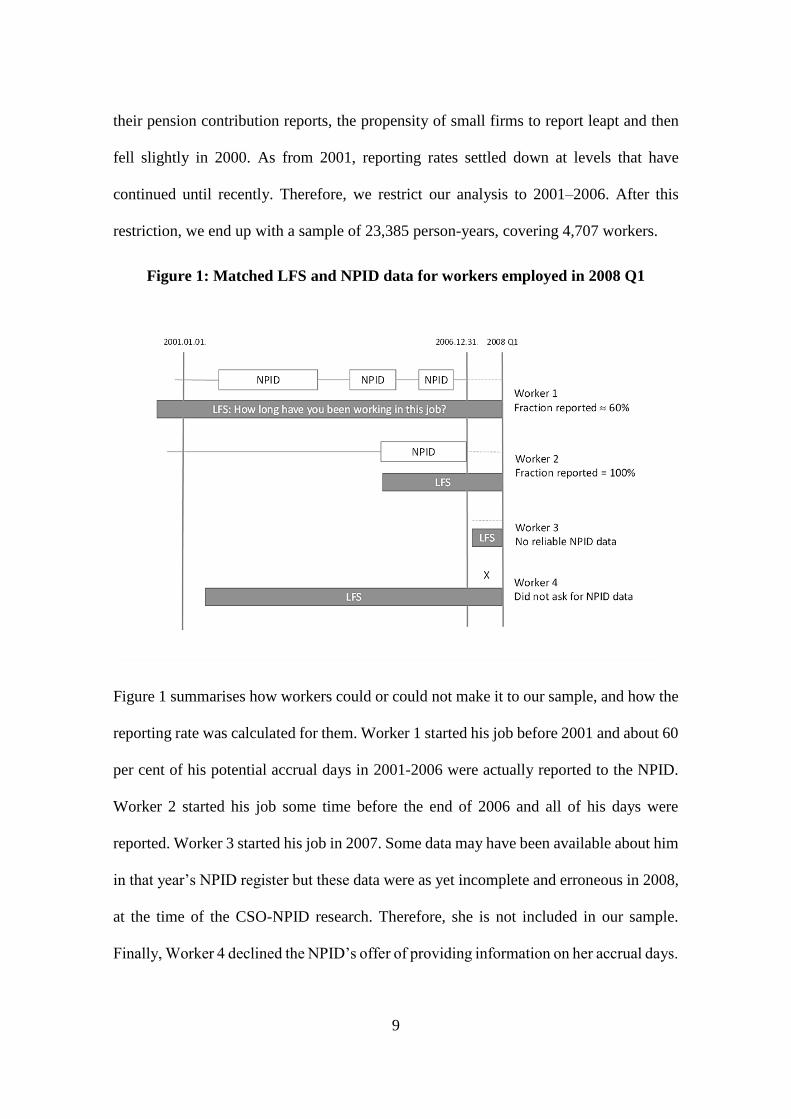
Figure 1: Matched LFS and NPID data for workers employed in 2008 Q1

Figure 1 summarises how workers could or could not make it to our sample, and how the

reporting rate was calculated for them. Worker 1 started his job before 2001 and about 60

per cent of his potential accrual days in 2001-2006 were actually reported to the NPID.

Worker 2 started his job some time before the end of 2006 and all of his days were

reported. Worker 3 started his job in 2007. Some data may have been available about him

in that year’s NPID register but these data were as yet incomplete and erroneous in 2008,

at the time of the CSO-NPID research. Therefore, she is not included in our sample.

Finally, Worker 4 declined the NPID’s offer of providing information on her accrual days.

10

2.2. Descriptive statistics

The fraction of unreported days in a given year shows that underreporting means no

reporting at all in the vast majority of cases. Instances where the firm did not report the

employment relationship at all in a given year accounted for 8 of the missing 9.5 per cent.

In the forthcoming sections we will regard a worker as ‘unreported’ if the fraction of her

reported days falls short of 50 per cent of all days in a given year – the average of this

dummy variable (9.2 per cent) is roughly the same as the ratio of unreported days (9.5 per

cent). However, the choice of the threshold only marginally alters our results.

According to Table 1, which displays the duration of unreported spells among workers

observed throughout 2001-2006, around 87 per cent of workers were always reported and

13 per cent were unreported at least once. There are three sizeable unreported groups:

around 50 per cent of them were permanently unreported, 25 per cent had a single

unreported year, and a further 25 per cent were unreported 2–5 times (6.5, 3.2 and 3.5 per

cent, respectively). Single-year and permanent non-reporting dominate in groups

observed for less than six years as well.

Table 1: The distribution of the number of unreported years among workers

observed for six years in the sample

Number of unreported years

0 1 2 3 4 5 6 Total

Per cent 86.7 3.2 1.3 0.8 0.6 0.8 6.5 100.0

Number

of workers

2,735 102 42 24 19 26 206 3,154

Note: workers in the matched LFS–NPID sample, who were observed in the whole period of

2001-2006. An unreported year means that less than half of the workdays are reported.

Transition probabilities between reported and unreported spells are displayed in Table 2

for those who were declared to the authorities at least once during their observed

employment period. On average, 1.1 per cent of reported workers became unreported in

11

the next period, and around half of the temporarily (i.e. not permanently) unreported

workers returned to a reported state one year later. The probabilities of returning to

reported work after one year, after more than one year, or – in the case of a left-censored

duration – after an unknown number of unreported years are around 40–50 per cent, and

do not differ significantly from each other,5 suggesting that the dynamics of temporary

non-reporting follows a Markov chain, with an average duration of two years in the

unreported state. There is one exception to this simple Markov rule: people who were

unreported in their first full year in their current job had a significantly higher (around 80

per cent) probability of transition to reported work after that year (Table 2). This will be

taken into account in model building.

Table 2: Transition probabilities between reported and unreported years among

workers who were reported at least once during their observed employment period

Last year If last year = unreported

Reported Unreported If previous unreported spell If tenure

= 1 year This year = 1 year > 1 year unknown

Reported 98.9% 49.0% 47% 38% 43% 79%

Unreported 1.1% 51.0% 53% 62% 57% 21%

Total 100.0% 100.0% 100% 100% 100% 100%

[16,940] [528] [137] [220] [68] [103]

Note: workers in the matched LFS–NPID sample, who were reported at least one during their

observed employment spell. The numbers of person-years by column are shown in brackets.

An unreported spell has unknown duration if it is left-censored. Tenure refers to the number of

years in the current job.

Table 3 summarizes average non-reporting rates in selected groups. Men are more likely

to be unreported, and are much more likely than women to be permanently unreported.

Undeclared work occurs most frequently among workers with secondary education (some

of them awaiting college admission) and least frequently among those with a university

degree; the differences by education are larger for permanent non-reporting. The

5 Homogeneity of the three distributions is not rejected by a chi-squared test (p-value is 0.22).

12

reporting rates are low for the self-employed; very low for casual workers; and below

average among farmers, skilled service and construction workers, porters, guards and

people doing elementary jobs. Part-timers are less likely to be reported than are full-

timers. Undeclared work is very frequent in telework. Also, people in their first full year

in their current job are about 3 percentage points more likely to be unreported than other

workers.

Table 3: Average non-reporting rates in the estimation sample (per cent)

Non-reporting rate Unreported

days

Unreported

year

Always

unreported

Transitorily

unreported*

Average 9.5 9.2 6.6 2.9

Gender

Male 13.4 13.1 9.6 3.5

Female 5.7 5.4 3.5 2.3

Age (2006 for ‘always unreported’)

15–29 years 12.6 11.9 7.4 4.3

30–49 years 9.0 8.8 6.7 2.6

50+ years 9.6 9.4 6.0 3.3

Level of education (2008)

Primary or less (0–8 classes) 9.2 8.8 6.5 3.1

Apprentice-based vocational 10.3 9.9 7.0 3.3

Vocational or general secondary 10.6 10.4 7.7 2.6

College 6.5 6.4 3.9 2.7

University 5.1 5.0 2.8 2.0

Type of employment relationship

(2008)

Employee 7.0 6.7 4.8 2.2

Employee of a sole proprietor 15.1 14.0 6.7 8.2

Casual worker 90.5 92.9 88.9 50.0

Self-employed 27.6 27.4 21.8 7.2

Member of an unincorporated

company

7.7 7.5 4.7 3.2

Occupation (2008, in order of non-reporting)

Agricultural 38.9 38.4 32.0 9.0

Skilled service workers 27.0 26.8 24.0 3.3

Skilled construction workers 14.1 13.2 8.8 5.2

Porters, guards 13.4 11.9 7.6 4.2

Professionals (except teachers and

doctors)

11.4 11.4 7.7 4.0

Elementary 11.3 10.5 7.0 4.3

Drivers 9.8 9.6 6.9 2.3

Skilled blue collars in trade and

catering

7.7 7.0 3.2 3.6

Skilled industrial workers 7.5 7.3 4.9 2.6

Administrators 7.2 7.1 5.2 2.7

13

Technicians 6.3 6.2 5.4 1.4

Cleaners 5.4 5.1 2.6 3.1

Managers 5.0 4.8 1.7 3.2

Office clerks 4.7 4.4 2.4 1.6

Machine operators and assemblers 4.3 3.9 3.4 1.3

Teachers and doctors 2.8 2.6 1.1 1.5

Work schedule (2008)

Part-time 31.7 30.8 19.8 11.8

Evening, night and weekend work 13.5 13.2 9.5 3.6

Telework 34.8 34.5 27.4 8.4

Irregular work pattern 17.5 17.1 12.7 4.2

Tenure in current job

First full year 12.9 11.7 - 5.9

More than one year 9.2 9.0 - 2.6

Firm size (number of workers, 2008)

1 34.8 34.8 28.0 9.4

2–4 12.0 11.4 7.7 4.5

5–10 5.6 5.2 2.4 3.2

does not know (but < 11) 13.7 13.9 8.5 4.8

11 or more 7.2 7.0 5.1 2.2

Firm ownership (2008)

Domestic (<=50% foreign) 10.4 10.1 7.2 3.2

Foreign (>50% foreign) 3.4 3.0 2.5 1.0

Region (2008)

Budapest 12.9 12.8 9.3 5.3

Rest of the country 9.4 9.1 6.5 2.8

Note: matched LFS–NPID sample.

Unreported year = less than half of the workdays are reported in a given year.

Always unreported = never reported during the observed employment spell.

Transitorily unreported = unreported years among workers who were reported at least once during

their observed employment period.

The ratios of unreported days, unreported years and transitorily unreported years are given as

percentages of person-years. The always unreported ratio is given as a percentage of the number

of workers. Hence, the ‘always’ and ‘transitory’ columns do not add up exactly to the total

column.

All explanatory variables except for age and tenure refer to year 2008 measurements in LFS.

They are time-invariant in most cases because the job of the workers did not change during the

observed period. For the ‘always unreported’ dummy, age is categorized according to its 2006

value.

Number of observations: 23,385 person-years covering 4,707 workers.

Foreign-owned firms have a much lower non-reporting rate than domestically owned

firms (3 versus 10 per cent). The share of unreported days does not exceed 7 per cent in

firms that employ five or more workers, but is around 12 per cent in firms employing 2–

14

4 workers and exceeds 30 per cent in sole proprietorships. Permanent undeclared work

seems to be more heterogeneous across groups than transitory non-reporting.

3. Methods

3.1. Baseline models

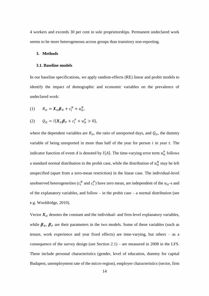
In our baseline specifications, we apply random-effects (RE) linear and probit models to

identify the impact of demographic and economic variables on the prevalence of

undeclared work:

(1) 𝑅𝑖𝑡 = 𝑿𝑖𝑡𝜷𝑁 + 𝑐𝑖𝑁 + 𝑢𝑖𝑡

𝑁,

(2) 𝑄𝑖𝑡 = 𝐼{𝑿𝑖𝑡𝜷𝑃 + 𝑐𝑖𝑃 + 𝑢𝑖𝑡

𝑃 > 0},

where the dependent variables are 𝑅𝑖𝑡, the ratio of unreported days, and 𝑄𝑖𝑡, the dummy

variable of being unreported in more than half of the year for person 𝑖 in year 𝑡. The

indicator function of event 𝐴 is denoted by 𝐼{𝐴}. The time-varying error term 𝑢𝑖𝑡𝑃 follows

a standard normal distribution in the probit case, while the distribution of 𝑢𝑖𝑡𝑁 may be left

unspecified (apart from a zero-mean restriction) in the linear case. The individual-level

unobserved heterogeneities (𝑐𝑖𝑁 and 𝑐𝑖

𝑃) have zero mean, are independent of the 𝑢𝑖𝑡-s and

of the explanatory variables, and follow – in the probit case – a normal distribution (see

e.g. Wooldridge, 2010).

Vector 𝑿𝑖𝑡 denotes the constant and the individual- and firm-level explanatory variables,

while 𝜷𝑁, 𝜷𝑃 are their parameters in the two models. Some of these variables (such as

tenure, work experience and year fixed effects) are time-varying, but others – as a

consequence of the survey design (see Section 2.1) – are measured in 2008 in the LFS.

These include personal characteristics (gender, level of education, dummy for capital

Budapest, unemployment rate of the micro-region), employer characteristics (sector, firm

15

size, firm ownership), type of employment and other employment variables (part-time

and atypical employment, telework, irregular work patterns). For the full list of variables,

see Table 4.

The majority of the above variables are either fixed in time (such as gender) or can be

treated as time-invariant because they refer to the individual’s work history within the

same firm (e.g. sector of the firm). Nevertheless, some variables (such as firm size, firm

ownership or type of employment) may have changed during the employment spell, and

this should be taken into account when interpreting the parameter estimates.

We estimate the RE linear model by RE-GLS, and display autocorrelation- and

heteroscedasticity-robust standard errors. We estimate the RE probit model using

maximum simulated likelihood (MSL) with adaptive Gauss–Hermite quadrature.6 To

compare results with the RE linear model, we also calculate the average marginal effects

of the variables on Pr(𝑄𝑖𝑡 = 1) from the RE probit model, where we integrate out the 𝑐𝑖𝑃

random effects.7

3.2. Model with endogenous selection

As described in detail in Section 2.1, selection into the panel dataset was non-random.

The incentive for an individual to obtain her official employment history is likely to have

been directly related to the time spent undeclared, the dependent variable in the equations.

Hence the parameter estimates on the selected sample are not necessarily consistent. This

is a Heckman-type selection problem, and the solution is to find a suitable instrumental

6 The likelihood function in the RE probit model is given as an integral with respect to the unobserved

heterogeneity 𝑐𝑖𝑃. In the MSL procedure this is approximated with adaptive Gauss–Hermite quadrature

and then maximized. We use 12 integration points, but the results are not sensitive to this choice.

Technically, the estimates are obtained with the xtprobit command of the Stata software (version 12). 7 The average marginal effects are calculated using the gllapred command of the GLLAMM package of

Stata, after bootstrapping the estimated model 1,000 times.

16

variable (IV) that influences the sampling probability, but otherwise can be treated as

random in relation to the prevalence of undeclared work. Since the LFS is a rotating panel,

where units are followed for up to six consecutive quarters, a suitable IV is the sequence

number of the visit of the pollster, when she asked the respondent for permission to be

included in the matched LFS–NPID sample. On average, the first visit of the pollster takes

much longer and is more elaborate than subsequent visits, because it takes time to get

acquainted with the sampled household, give the members an overview of the LFS and

inform them of the possibility to obtain information about their accrual years. Hence we

expect – and in fact we find (see Table A1 in Appendix) – that the first LFS visit is

associated with a greater probability of getting into the matched sample than are

subsequent visits, even after controlling for the observables. On the other hand, the wave

at which a respondent first appears in the LFS is obviously random, and hence the

sequence number of the LFS visit is unrelated to the respondent’s time spent undeclared.

We model selection into the matched LFS–NPID panel in a probit framework:

(3) 𝑆𝑖 = 𝐼{𝑿𝑖𝜹 + 𝑍𝑖𝜂 + 𝑣𝑖 > 0},

where 𝑆𝑖 denotes the dummy variable for being included in the matched LFS–NPID

sample, 𝑍𝑖 is the above IV, 𝑿𝑖 is the vector of observables in year 2006 (i.e. 𝑿𝑖 = 𝑿𝑖,2006),

which are all calculated from the LFS and hence are observed for all respondents, not just

for those in the matched sample, 𝜹 and 𝜂 are the corresponding parameters, and 𝑣𝑖 is a

standard normally distributed random variable.

17

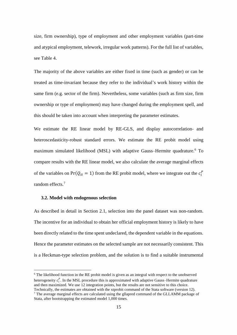
The structural equation for the dummy variable of undeclared work is given by the panel

probit model (equation (2)),8 but data for that equation are only available on the matched

sample (𝑆𝑖 = 1). In the model of endogenous selection, the two equations ((2) and (3))

are related by the assumption that

(4) corr(𝑣𝑖, 𝑐𝑖𝑃) = 𝜌.

If 𝜌 = 0, then equation (3) does not provide additional information on the structural

equation (2), but otherwise the two equations should be tackled jointly. We estimate the

system with maximum simulated likelihood, using adaptive quadrature.9 We calculate the

average marginal effects of the explanatory variables on Pr(𝑄𝑖𝑡 = 1), with the 𝑐𝑖𝑃 random

effects integrated out.

3.3. Separating permanent and transitory non-reporting

The above panel regressions do not explicitly model the time series properties of the non-

reporting process, although such a dynamic model – if well specified – could not only be

used in long-term dynamic simulations, but would also give more efficient estimates of

the effects of observables on undeclared work. The descriptive results in Tables 1 and 2

suggest that 𝑄𝑖𝑡, the dummy for undeclared work,10 follows a two-regime model: either

𝑄𝑖𝑡 = 1 holds for all years (permanent undeclared work) for a particular person, or 𝑄𝑖𝑡 is

– conditionally on the observables – a Markov chain (transitory undeclared work).

8 We do not use the linear specification (equation (1)) in models with endogenous selection, because the

estimation of such models depends crucially on distributional assumptions imposed on the error terms

(e.g. normality). 𝑅𝑖𝑡 is close to binary, and hence a binary model on 𝑄𝑖𝑡 is more appropriate. 9 Technically, the system is estimated using the GLLAMM package of the Stata software (Rabe-Hesketh

et al., 2004). 10 To keep the model structure relatively simple, we do not incorporate endogenous selection into the two-

regime model. According to Section 4.2, the model with endogenous selection yields qualitatively similar

results to the baseline ones.

18

More formally, let person i have explanatory variables 𝑿𝑖𝑡 in year 𝑡 (and in particular the

tenure in her current job in years, 𝐶𝑖𝑡), time-independent explanatory variables 𝑿𝑖,11 and

let us denote her latent (unobservable) regime by 𝐽𝑖, which can take value 1 (permanent

non-reporting) or 0 (transitory non-reporting). The probability of the permanent regime

is given by:

(5) Pr(𝐽𝑖 = 1 | 𝑿𝑖) = Φ(𝑿𝑖𝜷𝑍),

where Φ stands for the standard normal distribution function and 𝜷𝑍 is the parameter

vector describing the probability of permanent undeclared work.

The conditional probability of being undeclared is trivial for the permanent regime:

(6) Pr(𝑄𝑖𝑡 = 1 | 𝐽𝑖 = 1) = 1

while it is given as a function of the previous year’s state for the transitory regime:

(7) Pr(𝑄𝑖𝑡 = 1 |(𝑄𝑖,𝑡−1 = 0 or 𝐶𝑖𝑡 = 1), 𝐽𝑖 = 0, 𝑿𝑖𝑡) = Φ(𝑿𝑖𝑡𝜷𝑇) = 𝑝𝑖𝑡(01)

= 1 −

𝑝𝑖𝑡(00)

(8) Pr(𝑄𝑖𝑡 = 1 | 𝑄𝑖,𝑡−1 = 1, 𝐽𝑖 = 0, 𝑿𝑖𝑡) = 1 − Φ(𝑟0 + 𝑟1 ∗ 𝐼{𝐶𝑖𝑡 = 2}) =

= 𝑝𝑖𝑡(11)

= 1 − 𝑝𝑖𝑡(10)

,

where 𝜷𝑇 is the parameter vector determining the transition probability from the reported

to the unreported state, while the transition probability in the other direction is given by

Φ(𝑟0) in general and Φ(𝑟0 + 𝑟1) specifically after the first full year of tenure. The

probabilities in the first year of tenure (i.e. when 𝐶𝑖𝑡 = 1 and hence 𝑄𝑖,𝑡−1 is not defined)

are formally the same as for 𝑄𝑖,𝑡−1 = 0, but in practice they may differ because 𝑿𝑖𝑡

11 The notation here differs slightly from the previous section because 𝑿𝑖 now does not contain the year

2006 values of the time-varying variables (work experience and tenure).

19

contains 𝐶𝑖𝑡. Finally, 𝑝𝑖𝑡(01)

, 𝑝𝑖𝑡(00)

, 𝑝𝑖𝑡(11)

and 𝑝𝑖𝑡(10)

are just short notations for the

corresponding transition probabilities. Because of the small sample size in transitory non-

reporting (see Table 2), we do not model 𝑝𝑖𝑡(11)

as a function of observables beyond 𝐶𝑖𝑡.

Although 𝐽𝑖 is not observed (a worker can be unreported by chance throughout her

observed employment spell, even if she belongs to the transitory regime), the model can

be estimated by maximum likelihood. Indeed, the likelihood function can be obtained by

distinguishing between the cases of being reported at least once and never being reported.

We present the details in Appendix B.

After estimating the two-regime model with maximum likelihood, we also calculate the

average marginal effects of the covariates on the permanent and transitory non-reporting

probabilities, using the probit link functions.

4. Results

4.1. Determinants of undeclared work

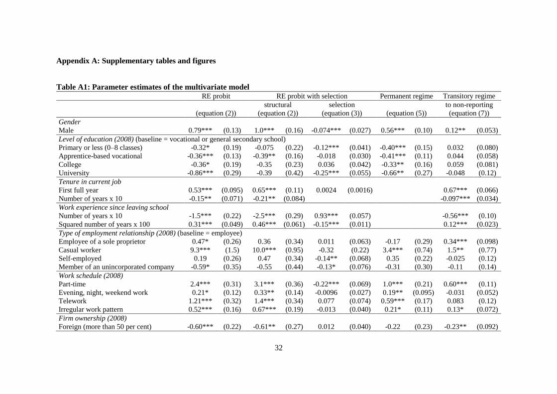
Table 4 displays the average marginal effects and Table A1 in Appendix the parameter

estimates of the RE linear and RE probit models (equations (1) and (2)), the RE probit

model with endogenous selection (equations (2)–(4) estimated as a system), and the two-

regime model that separates permanent and transitory undeclared work (equations (5)–

(8)).

As expected, the correlation between the error terms of the selection and the structural

equation in the endogenous model is significantly negative (𝜌 ≈ −0.5 in equation (4), see

the last row in Table A1), i.e. undeclared workers were less likely to allow the researchers

20

to obtain their official employment history. However, the majority of the marginal effect

estimates are similar in the RE probit models with and without endogenous selection,

hence we summarize the results from these models together.

According to Table 4, the average probability of belonging to the permanent regime was

around 5.6 per cent in the two-regime model. This is somewhat smaller than the observed

ratio of never-reported respondents (see Table 1), because some workers in the transitory

regime happen to be unreported during their whole observed period. If a worker was in

the transitory regime, her average transition probability was 1.8 per cent from the reported

to the non-reported state, and 36 per cent in the other direction (64 per cent after the first

full year of tenure at the current employer, and 34 per cent otherwise). We can simulate

the transitions in our six-year-wide window of observation and find that the average

probability of being in the non-reported state – conditionally on being in the transitory

regime – was around 3.7 per cent. Taking permanent and transitory non-reporting

together, the average simulated ratio of being unreported in a given year is around 9.0 per

cent, in good accordance with the observed ratio. Further details of goodness of fit of the

two-regime model are given in Section 4.3.

According to Table 4, the models indicate a higher than average ratio and probability of

undeclared work where this is expected on the basis of the predictions of theoretical

models and everyday experience. After controlling for other variables, males are 3–4

percentage points more likely than females to perform undeclared work, which can

possibly be explained by the higher risk aversion of females (Eckel and Grossman 2008).

Differences by gender are much larger in permanent than in transitory undeclared work.

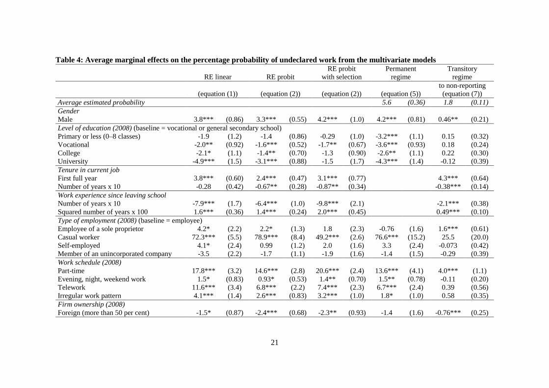
21

Table 4: Average marginal effects on the percentage probability of undeclared work from the multivariate models

RE linear RE probit

RE probit

with selection

Permanent

regime

Transitory

regime

(equation (1)) (equation (2)) (equation (2)) (equation (5))

to non-reporting

(equation (7))

Average estimated probability 5.6 (0.36) 1.8 (0.11)

Gender

Male 3.8*** (0.86) 3.3*** (0.55) 4.2*** (1.0) 4.2*** (0.81) 0.46** (0.21)

Level of education (2008) (baseline = vocational or general secondary school)

Primary or less (0–8 classes) -1.9 (1.2) -1.4 (0.86) -0.29 (1.0) -3.2*** (1.1) 0.15 (0.32)

Vocational -2.0** (0.92) -1.6*** (0.52) -1.7** (0.67) -3.6*** (0.93) 0.18 (0.24)

College -2.1* (1.1) -1.4** (0.70) -1.3 (0.90) -2.6** (1.1) 0.22 (0.30)

University -4.9*** (1.5) -3.1*** (0.88) -1.5 (1.7) -4.3*** (1.4) -0.12 (0.39)

Tenure in current job

First full year 3.8*** (0.60) 2.4*** (0.47) 3.1*** (0.77) 4.3*** (0.64)

Number of years x 10 -0.28 (0.42) -0.67** (0.28) -0.87** (0.34) -0.38*** (0.14)

Work experience since leaving school

Number of years x 10 -7.9*** (1.7) -6.4*** (1.0) -9.8*** (2.1) -2.1*** (0.38)

Squared number of years x 100 1.6*** (0.36) 1.4*** (0.24) 2.0*** (0.45) 0.49*** (0.10)

Type of employment (2008) (baseline = employee)

Employee of a sole proprietor 4.2* (2.2) 2.2* (1.3) 1.8 (2.3) -0.76 (1.6) 1.6*** (0.61)

Casual worker 72.3*** (5.5) 78.9*** (8.4) 49.2*** (2.6) 76.6*** (15.2) 25.5 (20.0)

Self-employed 4.1* (2.4) 0.99 (1.2) 2.0 (1.6) 3.3 (2.4) -0.073 (0.42)

Member of an unincorporated company -3.5 (2.2) -1.7 (1.1) -1.9 (1.6) -1.4 (1.5) -0.29 (0.39)

Work schedule (2008)

Part-time 17.8*** (3.2) 14.6*** (2.8) 20.6*** (2.4) 13.6*** (4.1) 4.0*** (1.1)

Evening, night, weekend work 1.5* (0.83) 0.93* (0.53) 1.4** (0.70) 1.5** (0.78) -0.11 (0.20)

Telework 11.6*** (3.4) 6.8*** (2.2) 7.4*** (2.3) 6.7*** (2.4) 0.39 (0.56)

Irregular work pattern 4.1*** (1.4) 2.6*** (0.83) 3.2*** (1.0) 1.8* (1.0) 0.58 (0.35)

Firm ownership (2008)

Foreign (more than 50 per cent) -1.5* (0.87) -2.4*** (0.68) -2.3** (0.93) -1.4 (1.6) -0.76*** (0.25)

22

Firm size (number of employees, 2008) (baseline = more than 10)

1 15.7*** (3.1) 12.1*** (2.2) 18.3*** (2.4) 6.7** (3.2) 2.6*** (0.95)

2–4 1.5 (1.4) 1.7** (0.78) 2.1* (1.2) 0.85 (1.5) 0.37 (0.34)

5–10 -1.5 (1.2) -0.73 (0.65) -0.95 (0.93) -2.9** (1.1) 0.34 (0.32)

does not know (but < 11) 3.3 (4.4) 2.3 (2.3) 2.9 (3.7) 2.8 (4.0) -0.17 (0.71)

Economic sector (2008) (baseline = industry)

Agriculture 15.7*** (1.8) 9.9*** (0.96) 7.5*** (1.5) 9.8*** (1.9) 1.1*** (0.43)

Construction 3.3** (1.7) 2.6*** (1.0) 4.6** (1.9) 0.29 (1.4) 1.3*** (0.45)

Transportation 20.5*** (2.7) 13.9*** (1.3) 21.6*** (1.3) 15.5*** (2.4) 0.83** (0.40)

Trade and accommodation -0.85 (1.0) 0.012 (0.68) 1.7 (1.1) -1.0 (0.71) 0.21 (0.28)

Services 1.3 (1.2) 1.2 (0.76) 2.3* (1.3) 0.28 (0.94) 0.71** (0.32)

Education, health, public admin. 3.8*** (1.0) 2.5*** (0.63) 2.5*** (0.95) 3.2*** (0.89) 0.14 (0.21)

Region (2008)

Micro-regional unemployment rate 18.3** (7.8) 10.6** (5.3) 8.2 (6.6) 16.7** (6.8) -1.8 (2.0)

Capital Budapest 6.8*** (2.4) 5.6*** (1.8) 14.6*** (3.3) 6.4** (3.2) 1.0* (0.62)

Year (baseline = 2001)

Year: 2002 0.30 (0.28) 0.13 (0.45) 0.40 (0.48) -0.057 (0.32)

Year: 2003 -0.033 (0.32) -0.12 (0.42) 0.23 (0.48) 0.028 (0.34)

Year: 2004 -0.42 (0.35) -0.42 (0.48) 0.0016 (0.53) -0.41 (0.30)

Year: 2005 -0.75** (0.37) -0.97** (0.41) -0.53 (0.47) -0.50* (0.29)

Year: 2006 -0.63 (0.41) -0.63 (0.40) -0.082 (0.47) -0.17 (0.29)

to reporting

(equation (8))

Average estimated probability 35.8 (2.7)

First full year in current job 29.9 (5.0)

Note: matched LFS-NPID sample. Standard errors (SEs) are in parentheses. Notations for significance: *: p<0.1; **: p<0.05; ***: p<0.01.

Average marginal effects (AMEs) are based on the parameter estimates shown in Table A1. For the RE linear model, AMEs are equal to the estimated

parameters (and cluster-robust SEs are shown). AMEs and SEs for all other models were calculated by bootstrapping the estimated model 1,000 times.

The gllapred command of GLLAMM package of Stata was used for the RE probit models with and without selection.

All explanatory variables except for work experience and tenure refer to year 2008 measurements in LFS.

Number of person-years: 23,385. Number of people: 4,707.

23

Holding other factors fixed, undeclared work is most prevalent among people with

secondary education. Those with apprentice-based vocational or primary education and

college graduates report more working days (1–2 percentage points more), while the

figure for university graduates is 2–5 percentage points higher than for comparable people

with secondary education. The differences come exclusively from permanent undeclared

work, which in all other categories is 3–4 percentage points lower than among those with

secondary education; the coefficients for the transitory probability are not significant.

Thus education and permanent undeclared work are in a reverse U-shaped relationship.

Holding everything else fixed, new entrants are 2–4 percentage points more likely to be

engaged in undeclared work. This result, as well as the above-average probability of

transition to reported work after the first full year of tenure, may be explained by the fact

that – according to the LFS – the share of fixed-term contracts is much higher in the first

full year (16 per cent) than in subsequent years (less than 3 per cent on average). Hence

workers may start a job undeclared, on a fixed-term contract, and later become reported

when they switch to an open-ended contract. Also, young people and people near

retirement age are significantly more likely to be unreported: the probability of

undeclared work is lowest 25 years after leaving school.

Undeclared work is more prevalent in situations where the perceived chance of detection

is lower, or where information asymmetries between the employer and the employee may

be present, e.g. among casual workers (50–80 percentage points more prevalent), part-

time workers (15–21 percentage points), people doing telework or working from home

(7–12 percentage points) and people with an irregular work pattern (2–4 percentage

points). Again, the differences in magnitude are larger in permanent than in transitory

non-reporting, and in permanent non-reporting are highly significant.

24

Workers in micro-firms, with only a single employee, are about 12–20 percentage points

more likely to be unregistered (about 7 percentage points more likely to be permanently

undeclared and 3 percentage points more likely to move from the reported to the non-

reported state in the transitory regime). The differences between other firm size categories

are not significant. The probability of undeclared work in general (and permanent

undeclared work in particular) is much higher in agriculture (8–16 percentage points

higher) and transport (14–22 percentage points) than in industry, while construction and

personal services (education, health care) also show slightly higher probabilities. This last

result may be due to the presence of unregistered private teachers and health care

professionals. Areas affected by high unemployment (perhaps due to demand-side

factors, such as the high ratio of the minimum wage to the average wage) and Budapest

(perhaps due to the smaller role of personal interactions) face a significantly greater

prevalence of undeclared work. A 1 percentage point higher unemployment rate in a

micro-region increases permanent non-reporting by a substantial 0.1–0.2 percentage

points. There was no trend visible in the extent of undeclared work between 2001 and

2006.

Overall, there is much more heterogeneity in probability in the permanent than in the

transitory regime. Explanatory variables that are associated with economic incentives

(such as level of education) play a substantially larger role in determining permanent non-

reporting, while transitory non-reporting is rather random and is affected by proxies of

administrative difficulties and possible negligent behaviour on the part of employees or

employers (e.g. part-time or casual workers). In light of this, it is interesting to find that

– after controlling for other factors – foreign ownership has a significant negative effect

on temporary, but not on permanent undeclared work.

25

4.2. Goodness of fit and long-term simulations

Before simulating long-term scenarios of undeclared work at the individual level, using

our two-regime model, we first note that this simple model is indeed able to reproduce

the observed patterns of non-reporting in our sample. To show this, using the model we

simulated undeclared work scenarios many times for each worker in the sample, and

calculated the distribution of the number of undeclared years. Table A2 in the Appendix

displays the mean, standard deviation and 5 per cent and 95 per cent quantiles of the

simulated ratios of workers who are undeclared for exactly 0, 1, …, 6 years. All but one

of the observed ratios are within the 5 per cent and 95 per cent simulated quantiles, and

the remaining case is within the corresponding 1 per cent and 99 per cent quantiles. Not

surprisingly, a formal chi-square test does not reject – even at the 10 per cent level – that

the observed distribution of undeclared years comes from the model-predicted

distribution. Thus the model captures two important patterns – the distinction between

permanent and transitory non-reporting and the mild persistence of transitory non-

reporting.

In our long-term simulations we generate individual undeclared work patterns for ten

years because, according to the LFS, a worker spends ten consecutive years on average

in the same job, provided she has spent at least two years there. Figure A3 in Appendix

displays the simulated distribution of the number of undeclared years in a ten-year

window for workers who were in the sample throughout the period 2001–2006, split by

their levels of education (lower than secondary, secondary and tertiary). Although the

average time spent undeclared during the ten-year window is 1.0 years for workers with

at most secondary education and 0.5 years for those with tertiary education, the

differences are substantially larger for permanent non-reporting: 6.1, 7.5 and 2.8 per cent

26

of workers from the three groups are never reported to the authorities in the ten-year

simulated window. This illustrates that the long-term burden of undeclared work is more

variable across people and socio-economic groups than cross-sectional differences would

suggest, because a typical undeclared worker is not sporadically, but rather permanently

unreported to the pension authorities.

5. Conclusions

In this paper we used a unique set of matched administrative and survey data to analyse

unreported employment at the individual level in Hungary, with the help of random-

effects panel models with endogenous selection and with a two-regime dynamic model.

We found that about 10 per cent of working time reported in the LFS by permanently

employed workers did not appear in the NPID register in 2001–2006. We estimated that

only about one-sixth of the discrepancy could be attributed to breaks in work during

employment relationships perceived as continuous by the LFS respondents.

These estimates of undeclared work are substantial, but smaller than the figures obtained

by comparing aggregate LFS and NPID employment data, which yield 16–17 per cent for

undeclared work in Hungary in 2001–2006 (Elek et al., 2009 and Benedek et al., 2013

for 2001–2005; own calculations for 2006). To control for the differences between our

restricted sample and the original LFS sample, we can use our model without year

dummies to predict the probability of undeclared work for each member of the 2008q1

LFS sample and obtain an undeclared work ratio of 11 per cent, still falling short of 16-

17 per cent. The remaining difference between the micro-level and the aggregate data

may come from two sources. First, we cannot control for the possibly higher prevalence

27

of undeclared work among workers whose completed tenure will be at most two years at

the end of their job spell – but they make up less than one tenth of the employment stock

at any time according to LFS. Second, the micro-level NPID data used here were quality-

checked and supplemented by NPID personnel using both computer-based and paper-

based information, which implies higher administrative employment and lower estimate

of unregistered employment.

Despite these differences, our results reinforce the idea that the labour input method

advocated in various European countries and at the EU level (GHK/FGB, 2009), can be

a simple, yet reliable method for estimating the size and evolution of informal

employment, although it tends to overestimate the true magnitude of black work by a few

percentage points, since some administrative records are missing for technical reasons.

The estimated effects of individual, firm-specific and regional variables – especially on

permanent undeclared work – suggest that non-reporting is a sign of black work, rather

than a result of technical failure. Importantly, we observed below-average reporting rates

in part-time work, non-standard work patterns, work at home and telework – various

forms of ‘atypical employment’ that are gaining ground in European labour markets. Our

results on lower reporting rates among males, in small firms and in some sectors such as

agriculture roughly coincide with the findings of other studies on undeclared work (e.g.

survey-based results in European Commission, 2014, for the EU, and Semjén et al., 2009,

for Hungary covering roughly the same period) and on more general forms of tax evasion,

such as wage underreporting and envelope wages (Meriküll and Staehr, 2010, for the

Baltic states; Elek et al., 2012, for Hungary). Education and undeclared work seem to be

in a reverse U-shaped relationship (see Meriküll and Staehr, 2010; Elek et al., 2012;

Paulus, 2015, for the effect of education on some other forms of tax evasion).

28

The findings have clear implications for health care and pension eligibility. Workers

whose administrative data are missing (for whatever reason) are only entitled to

emergency treatment unless they insure themselves on an individual basis (which rarely

happens in Hungary). We found the proportion of such workers to be quite high (about 1

in 10) – even in a sample that excluded employment spells of less than two years.

Expected pensions are also affected by non-reporting, and we could examine this with

our panel data. We found that about 6 per cent of workers were permanently undeclared.

Across a 40-year labour market career, employees who are unreported for their whole

tenure in a job (ten years on average) receive a pension that is about 15 per cent lower

than their fully reported counterparts, according to recent Hungarian rules (Pénzügyi

tudakozó, 2016). However, people permanently unreported in a ten-year time window

have a high probability of being unreported before and after, too; and so their total loss is

even higher.

Finally, as a more technical conclusion, we found that explicitly modelling the dynamics

of the dependent variable in a panel data setting not only gives greater insight into the

data-generating process, but may also yield more efficient parameter estimates than

simple panel data methods – in our case, some variables became significant only after

permanent and transitory non-reporting were separated.

29

References

Abowd JM, Stinson MH. 2013. Estimating measurement error in annual job earnings: a

comparison of survey and administrative data. Review of Economics and

Statistics 95(5): 1451–1467. DOI: 10.1162/REST_a_00352

Baldassarini A. 2007. The Italian approach of measuring undeclared work: description

and main strengths. Seminar on measurement of undeclared work, organized by

DG EMPL. Presentation, Brussels, December.

ec.europa.eu/social/BlobServlet?docId=2770&langId=en (accessed: 1st June

2016)

Baldini M, Bosi P, Lalla M. 2009. Tax evasion and misreporting in income tax returns

and household income surveys. Politica Economica 25(3): 333–348. DOI:

10.1429/30792

Bálint M, Köllő J, Molnár Gy. 2010. Accrual years and the life cycle. (in Hungarian).

Statisztikai Szemle 88(6): 623–647.

Benedek D, Elek P, Köllő J. 2013. Tax avoidance, tax evasion, black and grey

employment. In The Hungarian Labour Market, Review and Analysis 2013,

Fazekas K, Benczúr P, Telegdy Á (eds), pp. 161-187. Hungarian Academy of

Sciences Institute of Economics: Budapest.

http://econ.core.hu/file/download/HLM2013/TheHungarianLabourMarket_2013

_InFocusI.pdf (acessed: 1st June 2016)

Buehn A, Schneider F. 2012. Shadow economies around the world: novel insights,

accepted knowledge, and new estimates. International Tax and Public Finance

19(1): 139–171. DOI: 10.1007/s10797-011-9187-7

Cichocki S, Tyrowicz J. 2010. Shadow employment in post-transition: is informal

employment a matter of choice or no choice in Poland? Journal of Socio-

Economics 39(4): 527–535. DOI: 10.1016/j.socec.2010.03.003

Eckel CC, Grossman PJ. 2008. Men, women and risk aversion: experimental evidence.

In Handbook of Experimental Economics Results, Plott CR, Smith VL. (eds),

Vol. 1, Ch. 113, pp. 1061-1073. Elsevier. DOI: 10.1016/S1574-0722(07)00113-

8

Elek P, Köllő J, Reizer B, Szabó PA. 2012. Detecting wage underreporting using a

double-hurdle model. In Research in Labor Economics, Vol. 34 (Informal

Employment in Emerging and Transition Economies), Lehmann H, Tatsiramos

K. (eds.), Ch. 4, pp. 135-166. Emerald Group Publishing Limited. DOI:

10.1108/S0147-9121(2012)0000034007

Elek P, Scharle Á, Szabó B, Szabó PA. 2009. Measuring undeclared employment in

Hungary. (in Hungarian, with abstract in English). In Rejtett gazdaság. Be nem

jelentett foglalkoztatás és jövedelemeltitkolás – kormányzati lépések és a

gazdasági szereplők válaszai, Semjén A, Tóth IJ (eds), KTI Könyvek 11, pp.

84–102. Hungarian Academy of Sciences Institute of Economics: Budapest.

http://econ.core.hu/file/download/ktik11/ktik11_08_feketefoglalkoztatas.pdf

Abstract in English:

30

http://econ.core.hu/file/download/ktik11/ktik11_15_abstracts.pdf (accessed: 1st

June 2016)

European Commission. 2014. Undeclared work in the European Union. Special

Eurobarometer Report No. 402/wave EB79.2.

http://ec.europa.eu/public_opinion/archives/ebs/ebs_402_en.pdf (accessed: 1st

June 2016)

Feld LP, Larsen C. 2012. Undeclared work, deterrence and social norms: the case of

Germany. Springer.

GHK/FGB. 2009. Study on indirect measurement methods for undeclared work in the

EU (VC/2008/0305). European Commission, Directorate-General Employment,

Social Affairs and Equal Opportunities. Final Report submitted by GHK and

Fondazione G. Brodolini. December.

http://ec.europa.eu/social/BlobServlet?docId=4546&langId=en (accessed: 1st

June 2016)

Köllő J. 2015. An attempt to estimate informal employment based on unregistered work

observed in population surveys. (in Hungarian). Közgazdasági Szemle 62: 638–

651.

Meriküll J, Staehr K. 2010. Unreported employment and envelope wages in mid-

transition: comparing developments and causes in the Baltic countries.

Comparative Economic Studies 52(4): 637–670. DOI: doi:10.1057/ces.2010.17

Nastav B, Bojnec S. 2007. Shadow economy in Slovenia: the labour approach.

Managing Global Transitions 5: 193–208. http://www.fm-

kp.si/zalozba/ISSN/1581-6311/5_193-208.pdf (accessed: 1st June 2016)

Paulus A. 2015. Tax evasion and measurement error: an econometric analysis of survey

data linked with tax records. Institute for Social and Economic Research

Working Papers 2015/10.

Pénzügyi tudakozó. 2016. Pension calculation: how are accrual years calculated? (in

Hungarian) http://penzugyi-tudakozo.hu/nyugdij-szamitas-hogyan-szamoljak-a-

szolgalati-idot/ (accessed: 1st June 2016)

Pickhardt M, Prinz A. 2014. Behavioral dynamics of tax evasion: a survey. Journal of

Economic Psychology 40: 1–19. DOI: 10.1016/j.joep.2013.08.006

Pischke J.-S. 1995. Measurement error and earnings dynamics: some estimates from the

PSID validations study. Journal of Business and Economic Statistics 13(3): 305–

314. DOI: 10.1080/07350015.1995.10524604

Rabe-Hesketh S, Skrondal A, Pickles A. 2004. Generalized multilevel structural

equation modelling. Psychometrika 69(2): 167–190. DOI: 10.1007/BF02295939

Renooy P, Ivarsson S, van der Wusten-Gritsai O, Meijer R. 2004. Undeclared work in

an enlarged Union. Final report, European Commission Directorate-General for

Employment and Social Affairs, May. http://www.social-

law.net/IMG/pdf/undecl_work_final_en.pdf (accessed: 1st June 2016)

Schneider F. 2012. The shadow economy and work in the shadow: what do we (not)

know? IZA Discussion Paper, No. 6423.

31

Semjén A, Tóth IJ, Medgyesi M, Czibik Á. 2009. Tax evasion and corruption:

population involvement and acceptance. In Rejtett gazdaság. Be nem jelentett

foglalkoztatás és jövedelemeltitkolás – kormányzati lépések és a gazdasági

szereplők válaszai, Semjén A, Tóth IJ (eds), KTI Könyvek 11, pp. 228–258.

Hungarian Academy of Sciences Institute of Economics: Budapest.

http://econ.core.hu/file/download/ktik11/ktik11_14_lakossagi.pdf Abstract in

English: http://econ.core.hu/file/download/ktik11/ktik11_15_abstracts.pdf

(accessed: 1st June 2016).

Slemrod J, Yitzhaki S. 2002. Tax avoidance, evasion, and administration. In Handbook

of Public Economics, Auerbach AJ, Feldstein M. (eds), 1st edition, Vol. 3, No.

3, Ch. 22, pp. 1423-1470. Elsevier.

Williams CC. 2007. Tackling undeclared work in Europe: lessons from a study of

Ukraine. European Journal of Industrial Relations 13(2): 219–236. DOI:

10.1177/0959680107078254

Wooldridge JM. 2010. Econometric Analysis of Cross Section and Panel Data. 2nd

edition. MIT Press

Acknowledgements: The authors would like to thank Anikó Bíró, Márton Csillag and

Gábor Kézdi for useful comments on an earlier version of the paper. Péter Elek was

supported by the János Bolyai Research Scholarship of the Hungarian Academy of

Sciences.

32

Appendix A: Supplementary tables and figures

Table A1: Parameter estimates of the multivariate model RE probit RE probit with selection Permanent regime Transitory regime

(equation (2))

structural

(equation (2))

selection

(equation (3)) (equation (5))

to non-reporting

(equation (7))

Gender

Male 0.79*** (0.13) 1.0*** (0.16) -0.074*** (0.027) 0.56*** (0.10) 0.12** (0.053)

Level of education (2008) (baseline = vocational or general secondary school)

Primary or less (0–8 classes) -0.32* (0.19) -0.075 (0.22) -0.12*** (0.041) -0.40*** (0.15) 0.032 (0.080)

Apprentice-based vocational -0.36*** (0.13) -0.39** (0.16) -0.018 (0.030) -0.41*** (0.11) 0.044 (0.058)

College -0.36* (0.19) -0.35 (0.23) 0.036 (0.042) -0.33** (0.16) 0.059 (0.081)

University -0.86*** (0.29) -0.39 (0.42) -0.25*** (0.055) -0.66** (0.27) -0.048 (0.12)

Tenure in current job

First full year 0.53*** (0.095) 0.65*** (0.11) 0.0024 (0.0016) 0.67*** (0.066)

Number of years x 10 -0.15** (0.071) -0.21** (0.084) -0.097*** (0.034)

Work experience since leaving school

Number of years x 10 -1.5*** (0.22) -2.5*** (0.29) 0.93*** (0.057) -0.56*** (0.10)

Squared number of years x 100 0.31*** (0.049) 0.46*** (0.061) -0.15*** (0.011) 0.12*** (0.023)

Type of employment relationship (2008) (baseline = employee)

Employee of a sole proprietor 0.47* (0.26) 0.36 (0.34) 0.011 (0.063) -0.17 (0.29) 0.34*** (0.098)

Casual worker 9.3*** (1.5) 10.0*** (0.95) -0.32 (0.22) 3.4*** (0.74) 1.5** (0.77)

Self-employed 0.19 (0.26) 0.47 (0.34) -0.14** (0.068) 0.35 (0.22) -0.025 (0.12)

Member of an unincorporated company -0.59* (0.35) -0.55 (0.44) -0.13* (0.076) -0.31 (0.30) -0.11 (0.14)

Work schedule (2008)

Part-time 2.4*** (0.31) 3.1*** (0.36) -0.22*** (0.069) 1.0*** (0.21) 0.60*** (0.11)

Evening, night, weekend work 0.21* (0.12) 0.33** (0.14) -0.0096 (0.027) 0.19** (0.095) -0.031 (0.052)

Telework 1.21*** (0.32) 1.4*** (0.34) 0.077 (0.074) 0.59*** (0.17) 0.083 (0.12)

Irregular work pattern 0.52*** (0.16) 0.67*** (0.19) -0.013 (0.040) 0.21* (0.11) 0.13* (0.072)

Firm ownership (2008)

Foreign (more than 50 per cent) -0.60*** (0.22) -0.61** (0.27) 0.012 (0.040) -0.22 (0.23) -0.23** (0.092)

33

Firm size (number of employees, 2008) (baseline = more than 10)

1 2.0*** (0.32) 2.7*** (0.38) -0.049 (0.079) 0.58** (0.23) 0.47*** (0.13)

2–4 0.40** (0.19) 0.46* (0.24) -0.047 (0.046) 0.092 (0.18) 0.010 (0.084)

5–10 -0.17 (0.22) -0.26 (0.27) 0.034 (0.047) -0.74* (0.38) 0.091 (0.082)

does not know (but < 11) 0.51 (0.47) 0.63 (0.65) -0.15 (0.11) 0.26 (0.38) -0.098 (0.24)

Economic sector (2008) (baseline = industry)

Agriculture 1.9*** (0.20) 1.4*** (0.24) 0.26*** (0.053) 0.99*** (0.16) 0.28*** (0.090)

Construction 0.70*** (0.23) 1.1*** (0.28) -0.22*** (0.053) 0.0011 (0.30) 0.32*** (0.093)

Transportation 2.6*** (0.23) 3.2*** (0.26) -0.029 (0.054) 1.3*** (0.16) 0.23** (0.10)

Trade and accommodation 0.047 (0.21) 0.48* (0.25) -0.18*** (0.040) -0.37 (0.26) 0.059 (0.081)

Services 0.39* (0.21) 0.63** (0.28) -0.14*** (0.046) 0.047 (0.22) 0.20** (0.085)

Education, health, public admin. 0.77*** (0.18) 0.80*** (0.21) -0.036 (0.039) 0.61*** (0.16) 0.053 (0.078)

Region (2008)

Micro-regional unemployment rate 2.5** (1.1) 2.0 (1.3) 0.017*** (0.0025) 2.1** (0.85) -0.46 (0.50)

Capital Budapest 1.1*** (0.26) 2.3*** (0.41) -0.63*** (0.054) 0.56** (0.22) 0.21* (0.11)

Year (baseline = 2001)

Year: 2002 0.042 (0.097) 0.095 (0.11) -0.015 (0.076)

Year: 2003 -0.021 (0.097) 0.054 (0.11) 0.0022 (0.074)

Year: 2004 -0.099 (0.099) -0.0004 (0.11) -0.11 (0.076)

Year: 2005 -0.22** (0.10) -0.13 (0.11) -0.13* (0.077)

Year: 2006 -0.13 (0.10) -0.020 (0.12) -0.041 (0.071)

Exogenous variable in selection equation (2008)

Sequence number of LFS visit -0.035*** (0.0071)

Constant -4.4*** (0.32) -2.1*** (0.41) -1.9*** (0.085) -2.7*** (0.19) -1.8*** (0.14)

to reporting

(equation (8))

First full year in current job 0.77*** (0.13)

Constant -0.40*** (0.075)

𝜎(𝑐𝑖) 3.2*** (0.066) 6.9*** (0.42)

𝜌 (in equation (4)) -0.48*** (0.044)

Note: see Table 4. Standard errors are in parentheses. Notations for significance: *: p<0.1; **: p<0.05; ***: p<0.01.

See also Table 4 for the parameter estimates of the RE linear model. Additional parameter estimates of that model: 𝜎(𝑐𝑖) = 0.23 and 𝜎(𝑢𝑖𝑡) = 0.12.

34

Table A2: Descriptive statistics of the simulated ratios of workers undeclared for

exactly 𝒌 years (𝒌 = 𝟏, 𝟐, … , 𝟔) in the six-year period and the observed distribution

in the sample (in per cent)

Number of undeclared years (𝑘)

Ratios

(per cent)

0 1 2 3 4 5 6 Total

Observed 86.41 4.57 1.83 0.89 1.06 0.87 4.38 100.0

Simulated

Mean 85.73 4.85 2.11 1.29 0.98 0.73 4.31 100.0

S. D. 0.65 0.39 0.23 0.18 0.15 0.12 0.35

Quantiles

5% 84.62 4.26 1.74 1.00 0.73 0.57 3.76

95% 86.84 5.53 2.49 1.60 1.21 0.93 4.91

Note: simulation of non-reporting dummies based on observed characteristics of 4,707 workers

in the matched LFS–NPID sample for 2001–2006, using the two-regime model and taking into

account the variance-covariance matrix of its parameter estimates. Number of simulation draws:

1,000.

Figure A1: Reporting rates for employees of small and large firms (1995-2006)

Note: matched LFS–NPID sample for 1995–2006. Vertical lines indicate the years of two

regulatory changes on NPID reporting. In the paper we use data for 2001–2006.

50

60

70

80

90

100

per

cen

t

1995 1996 1997 1998 1999 2000 2001 2002 2003 2004 2005 2006year

at most 10 employees more than 10 employees

35

Figure A2: Simulated distribution of the number of unreported

years in a ten-year time window

Note: matched LFS–NPID sample. Level of education: lower = primary and apprentice-based

vocational, secondary = vocational and general secondary, tertiary = college or university.

Appendix B: Maximum likelihood estimation of the two-regime model

Let ti denote worker i’s first year in the sample (which can take values between 2001 and

2006) and let us use the notations 𝑝𝑖𝑡(𝑘)

= Pr(𝑄𝑖𝑡 = 𝑘 | 𝐽𝑖 = 0, 𝑿𝑖𝑡) for the probability of

transitory non-reporting (𝑘 = 1) and reporting (𝑘 = 0), respectively, at time 𝑡. If

∏ 𝑄𝑖𝑡2006𝑡=𝑡𝑖

= 0 (i.e. if the person is reported at least once), then for 𝑘𝑡 ∈ {0,1}

(𝑡 = 𝑡𝑖, … , 2006):

(9) Pr(⋂ {𝑄𝑖𝑡 = 𝑘𝑡} | {𝑿𝑖𝑡}2006𝑡=𝑡𝑖

) = (1 − Φ(𝑿𝑖𝜷𝑍)) ∗ 𝑝𝑖,𝑡𝑖

(𝑘𝑡𝑖)

∗ ∏ 𝑝𝑖𝑡(𝑘𝑡−1,𝑘𝑡)2006

𝑡=𝑡𝑖+1

and if ∏ 𝑄𝑖𝑡2006𝑡=𝑡𝑖

= 1 (i.e. if the person is never reported), then

05

10

75

80

85

90

ratio (

pe

r ce

nt)

0 1 2 3 4 5 6 7 8 9 10

lower secondary

tertiary

36

(10) Pr(⋂ {𝑄𝑖𝑡 = 1} | {𝑿𝑖𝑡}2006𝑡=𝑡𝑖

) = Φ(𝑿𝑖𝜷𝑍) + (1 − Φ(𝑿𝑖𝜷𝑍)) ∗ 𝑝𝑖,𝑡𝑖

(1)∗

∏ 𝑝𝑖𝑡(11)2006

𝑡=𝑡𝑖+1 .

The first term in the latter expression shows the contribution of the permanent regime;

the second term that of the transitory regime.

For workers who entered the sample at the start of their current job (i.e. for whom 𝐶𝑖,𝑡𝑖=

1), equation (7) implies that 𝑝𝑖,𝑡𝑖

(𝑘)= 𝑝𝑖,𝑡𝑖

(0,𝑘) and hence the likelihood calculation is complete

for them. However, the majority of our observations are left-censored because 𝐶𝑖,2001 >

1 for most workers who entered our sample in 2001. The missing observations from their

work history can be tackled, for instance, using the expectation-maximization (EM)

algorithm, or we can follow a computationally less intensive but equally satisfactory

approach. Indeed, we first note that 𝑝𝑖𝑡(1)

can be calculated recursively:

(11) 𝑝𝑖𝑡(1)

= 𝑝𝑖𝑡(11)

∗ 𝑝𝑖,𝑡−1(1)

+ 𝑝𝑖𝑡(01)

∗ (1 − 𝑝𝑖,𝑡−1(1)

),

hence, to obtain 𝑝𝑖,2001(1)

and 𝑝𝑖,2001(0)

– only they are needed in equations (9)–(10) for the

likelihood – we can go back to (for example) year 1997 and approximate 𝑝𝑖,1997(1)

as the

stationary distribution of the two-state Markov chain whose transition probabilities are

fixed at their 1997 levels:

(12) pi,1997(1)

≈ pi,1997(01)

(pi,1997(10)

+ pi,1997(01)

)⁄ .

This final step is only an approximation, because (1) the transition probabilities are

slightly time-varying and (2) the Markov chain may not have reached the stationary

distribution for some workers by 1997. Nevertheless, since the probability of return to the

reported state, pit(10)

, turns out to be relatively large in our case (see Section 4.1), the

37

corresponding Markov chain has good mixing properties, and it seems to be enough to go

back four years in time to get a satisfactory approximation for pi,2001(1)

in equations (9)–

(10). We note that the maximum likelihood estimates turn out to be almost identical,

irrespective of whether 1996, 1997 or 1998 is used as the start year in the approximation.